
Distinguishing Household Groupings within a Precinct Based on Energy Usage Patterns Using Machine Learning Analysis

1
Sustainability Policy Institute, School of Design and Built Environment, Curtin University, Building 418 Level 4, Kent St., Bentley, WA 6102, Australia
2
School of Electrical Engineering, Computer and Math Science, Curtin University, Building 314 Level 4, Kent St., Bentley, WA 6102, Australia
*
Author to whom correspondence should be addressed.
Energies 2023, 16(10), 4119; https://doi.org/10.3390/en16104119
Submission received: 6 April 2023
/
Revised: 9 May 2023
/
Accepted: 10 May 2023
/
Published: 16 May 2023
(This article belongs to the Topic Built Environment and Human Comfort)
Abstract
:The home can be a complex environment to understand, as well as to model and predict, due to inherent variability between people’s routines and practices. A one-size-fits-all approach does not consider people’s contextual and institutional influences that contribute to their daily routines. These contextual and institutional factors relate to the household structure and relationship between occupants, as well as the working lifestyle of the occupants. One household can consume resources and live quite differently compared to a similar size household with the same number of occupants due to these factors. Predictive analysis of consumption data can identify this difference to create household-specific modelling to predict occupant routines and practices. Using post-occupancy data from the Fairwater Living Laboratory in Sydney that monitored 39 homes built in a green-star community, this research has utilised machine learning approaches and a K-Means clustering method complemented by t-distributed Stochastic Neighbour Embedding (t-SNE) to show how households follow different daily routines and activities resulting in resource consumption. This analysis has identified energy usage patterns and household groupings with each group following similar daily routines and consumption. The comparison between modelling the precinct as a whole and modelling households individually shows how detail can be lost when aggregating household data at a precinct/community level. This detail can explain why policies or technologies are not as effective as their design due to ignoring the delicate aspects of household routines and practices. These household groupings can provide insight for policymakers to help them understand the different profiles that may be present in the community. These findings are useful for net-zero developments and decarbonization of the built environment through modelling occupant behaviour accurately and developing policies and technologies to suit.
1. Introduction
The built environment contributes a significant portion of total energy consumption worldwide, playing a major role in the transition to net zero. Household energy consumption contributes to environmental issues with approximately 38% of the total US carbon emissions generated by direct energy use from the residential environment [1]. Further adding to the problem is the high variance in household energy consumption that makes it difficult to reduce this impact across the population. The variance makes it difficult for energy prediction and management systems, intermittent energy supply, and policymaking to have a significant impact on reducing energy consumption.
Past research has estimated that up to 27% of current energy use can be saved through energy efficiency measures [2]. This consists of a combination of technological advances and behavioural changes [3]. This highlights the importance of understanding and influencing the behaviour and routines of households to improve energy use and encourage energy conservation [4]. Energy and environmental policies have targeted behaviour change to achieve household energy conservation [5]. This focus on behaviour or practice change is due to the high potential impact when compared to some technological changes [6]. These policies can influence energy conservation by changing the way energy is consumed within the home without investing in expensive technology.
The energy consumed by a residential home is affected by the physical properties of the house, the outdoor environment, and occupant behaviour, routines, and practices [7]. This outlines the complexity of the residential environment with a great deal of variation between homes relating to each of these aspects. Estimating energy consumption can be difficult as people have different comfort requirements, and ultimately, the thermal environment and occupant practices influence the total energy demand of the home [7]. Previous research has categorised occupant behavioural patterns based on occupancy status, the number of occupants, the location and activity of the occupants to estimate energy demand [8]. However, this may differ between households due to contextual or institutional factors, preventing a uniform understanding.
The residential sector faces the challenge of responding to demand and providing energy for households with a large diversity of occupant behavioural patterns [9]. Additionally, there are great financial barriers to large-scale monitoring, which restricts the ability to measure these diverse patterns. Advancements in smart meter technology have made this monitoring available to collect information to conduct occupant behavioural modelling or load forecasting. This raises an additional challenge with big data analysis that requires addressing [10,11]. A significant amount of research has been established to develop smart energy management systems and energy-intensive building systems controls (i.e., HVAC) [12,13]. Building modelling and automation systems have been developed using time-series data to achieve HVAC energy efficiency, thermal comfort and improved air quality [14,15].
Occupant behaviour has been studied extensively, relating people’s daily routines to social and psychological theories to understand the repetitive nature of people’s lifestyles. The concept of the Home System of Practice (HSOP) developed from the principles of Social Practice Theory (SPT) describes how in the home environment, routines are created based on occupants’ lifestyles and interactions, influencing the consumption of resources [16]. This paper utilises data analytical techniques to investigate the HSOP concept and identify the different routines people follow when they are at home. The objective of the paper is to evaluate whether homes within a precinct can be grouped based on their consumption patterns to provide insight into moving away from a one-size-fits-all solution and towards looking at the different consumer groups and developing a targeted solution for each of the groups.
This addressed current gaps in the research, including the need to understand occupant routines and practices in a systematic framework, linking occupant behaviour to socio-economic variables, and evaluating the role of the occupant in the effectiveness of policies [17]. A published systematic literature review has identified there is a lack of qualitative investigation of behaviour compared to the research into the quantitative aspect of behaviour [18]. Past work has established smart energy management systems and reviewed the potential of building system controls for energy-intensive activities (e.g., HVAC) [12,19]. This work focuses on the quantitative approach to smart energy systems and modelling energy consumption using predictive models [14,15]. These models are not built on using principles of HSOP and SPT and hence do not consider the complex nature of occupant behaviour. Ref. [20] showed the potential of using these social theories to complement the analysis from predictive models to evaluate energy usage patterns.
This paper will link the quantitative data with the qualitative data collected from the Fairwater Living Laboratory, a four-year study in Australia. The paper will use these data to identify household groupings within the Fairwater Living Laboratory that follow similar daily routines and energy consumption profiles. This paper identifies potential household groupings based on their energy behaviour and reinforces the influence of occupant behaviour on energy consumption. The findings contribute to the development of smart energy management systems by demonstrating that the end user must be considered during the design stage. This paper recommends adapting and changing the design and operation of these systems based on user groups’ consumption patterns that naturally occur within a residential energy system (i.e., precinct).
2. Theoretical Background
This section will review the social theories regarding the drivers of energy consumption within the home with a focus on the influences of occupant behaviours on household energy consumption. This will support the evaluation of the Fairwater Living Laboratory precinct data.
2.1. Home System of Practice
The evolution of behavioural and psychological models and theories of consumers have aimed to understand the behaviours of occupants at home. Some models and theories include the Theory of Cognitive Dissonance [21], the Theory of Planned Behaviour [22], and the Social Practice Theory (SPT) [23]. These models have been adopted by researchers to explore household energy consumption routines and practices and identify factors that influence this consumption [24,25,26,27,28]. From this, intervention strategies have been developed, aimed at changing people’s energy use behaviour resulting in energy savings and conservation [29,30,31,32,33,34].
These theories and models are used in this paper as backbones for the development of the methodology and data analysis. Social Practice Theory aims to understand the way energy is consumed within the home to explain the temporal aspects of residential consumption [35]. This theory discusses how individuals live in a routinised way and perform similar activities at similar times resulting in consistent energy consumption [36]. The theory can assist in identifying practices that relate to significant resource consumption and understanding why people perform these practices in the way that they do [37,38,39,40]
The HSOP aims to provide an in-depth understanding of the interlocking relationships between multiple systems of social practices within a home [16]. A household occupied by several individuals can consist of many different routines and lifestyles that each individual follows. Individuals perform daily practices sequentially, making up their typical daily routines [16]. In some cases, the practices are shared among all the individuals within the home, and in other cases, they can be specific to the individual.
2.2. Occupant Behaviour and Lifestyles (Variation/Fluctuation)
Occupants play an important role in the built environment, with many methodologies being developed to identify and evaluate behaviour [41,42,43]. The impact on energy consumption is rather complex with many identified factors and determinants that range between households [44]. The interrelationship between routines, practices and resource consumption is linked back to the HSOP to explain the nature of the consumption.
The influence of occupant routines and lifestyles on the way energy is consumed within the home has been investigated in many research articles [44]. The behaviour of occupants can influence their consumption profiles differently resulting in variation in consumption across households [45]. Within the literature, there is a focus on how changes in occupant behaviour can impact their energy consumption [17,18,32,46]. The underlying principle of this focus is to encourage occupants to follow lifestyles and change their behaviour to positively influence the way they consume energy. However, a major limitation is a challenge of achieving permanent change in behaviour, with many studies observing occupants reverting to their normal behaviour patterns after some time [47].
The influence of behaviour and inherent variation in household energy consumption results in the home environment being a complex system that is difficult to model. Measuring energy consumption and developing typical consumption profiles for households [48,49] can make it possible to accurately model these environments [49,50]. This modelling can make assessments and predictions of energy consumption that can be useful for policymakers [24,51]. Additionally, predictions and forecasting can assist household or building energy management systems and increase the effectiveness of renewable energy generation technologies. However, these models can vary in accuracy when they do not consider varying occupant behaviours and lifestyles. The reasons for energy management systems and automation not being as effective due to the lifestyles and behaviours of the occupants are explored further in [52]
Other research has tried to develop behaviour models to quantitatively evaluate the impact of occupant behaviour [18,53]. This reinforces the influence of occupant behaviour on how energy is consumed within the residential sector. The analysis of the energy data from four buildings in Seattle from 1987 to 2002 demonstrated the impact of different lifestyles on energy consumption [54]. This is supported by the use of clustering analysis to examine the effects of different behaviour patterns on energy consumption showing significant attributes of the four clusters identified [18]. Further insight was provided by considering occupants’ schedules and family types, and lifestyle changes such as increased leisure time at home resulted in energy consumption changes [55]. These studies emphasise the influence of occupant behaviour and how the resultant energy consumption can fluctuate.
2.3. Occupant Behaviour Identification and Classification
Personal information about households and their characteristics can assist in evaluating behaviour patterns and classifications. Typically, this information includes gender, age, number of children, marital status, employment status (including working days), and income [7,29,49,53,56,57,58,59]. There are drawbacks to classifying behaviour on this information alone because there is no guarantee that similar personal characteristics will result in similar behaviour patterns [60]. It is difficult to classify behavioural patterns when data are collected through monitoring and surveying as the more complicated human characteristics such as personality, opinion, and emotional status are difficult to gauge through surveys [61]. This previous work supports the complex nature of the household environment and the uniqueness of each household in the way they live and consume energy.
Previous studies have been conducted that used clustering to recognise occupancy patterns. Four working occupancy patterns were identified in office buildings using this approach [62]. Occupant behaviour simulations have shown the link between the number of occupants and the energy demand of thermal and ventilation services [49]. Secondly, these simulations connected the use of artificial lighting, HVAC, and other appliances to occupancy patterns [34,63,64]. This paper adopts this clustering approach to identify common occupant behaviours in a residential precinct to evaluate whether households can be grouped based on their typical consumption and behaviour patterns.
Table 1 provides a summary of the work conducted in the literature and identifies the research gap that this paper aims to fill.
3. Methods
The following section describes the process undertaken in this paper, including the strategy for data collection, and the calculation and analysis undertaken.
3.1. Living Laboratory
This paper uses data collected from the Fairwater Living Laboratory (FLL) project based in the suburb of Blacktown, Sydney, New South Wales, Australia. This project was developed to evaluate the effectiveness of ground source heat pumps in residential homes to reduce energy consumption compared to typical heating and cooling systems. The FLL consisted of a sustainable housing precinct that was awarded the top 6-star Green Star Communities Rating under the Green Building Council of Australia’s accreditation scheme. The precinct consists of 850 homes with 39 of the homes subjected to detailed monitoring as a part of the study between 2019 to 2022.
This project used a multi-method approach that collected social and technical data of the occupants to provide information on the way the occupants consumed resources. These monitored homes were all owner-occupied and ranged between 2-to-5-bedroom houses.
Each home had its electrical energy use monitored at a circuit level, as well as the indoor environmental conditions such as the indoor temperature and humidity. The circuits that were monitored included the mains electricity, air conditioning, lights, power, oven, solar inverter, battery (if applicable), water (if applicable), garage, and loft (if applicable). These energy data were collected at 30 min intervals between 1 July 2019 to 1 January 2022.
3.2. Calculation Method
The energy data were used to identify groupings in the FLL based on the typical daily energy profiles of the 39 homes. These profiles were then grouped based on their shape and magnitude to evaluate whether homes within a precinct consume similar daily energy profiles. This method of analysis aims to provide better insight into precinct energy consumption compared to treating the precinct as a whole system. This assessment seeks to show the information that is lost or hidden when assessing the precinct performance of the whole system (aggregating household energy data) instead of breaking the precinct into different systems (household groupings).
The paper followed a three-step assessment of the energy data collected from the FLL:
- Statistical analysis
The analysis started by using simple statistical methods to show the difference in energy consumption across households at a high level. The time series data were aggregated into six categories: ‘Early Morning’ (00:00 to 05:00), ‘Morning’ (05:00 to 08:00, ‘Late Morning’ (08:00 to 12:00), ‘Afternoon’ (12:00 to 16:00), ‘Late Afternoon’ (16:00 to 19:00) and ‘Evening’ (19:00 to 00:00) to reduce the resolution and complexity of the data. The key metrics that were used included mean and standard deviation for each defined period. The analysis then focused on two households as case studies to gain a better understanding of the findings from this method of analysis. This highlights the different insights that can be gained from assessing the way energy is consumed at a precinct level and a household level. Simplifying the data into these periods and aggregating the household energy data into one dataset tells a high-level story of the precinct’s performance and the periods where consumption is high and low. However, it lacks detail and understanding of occupant patterns and lifestyles that are required when developing policies and energy technology.
- 2.
- k-Means clustering
The energy data collected from the study homes were analysed and assessed in two ways. The first way involved aggregating and summing all the individual household energy data into one dataset that represented the total energy consumption from the precinct as-a-whole. This dataset was used as a baseline for this methodology to demonstrate the patterns that can be identified from a precinct perspective. The dataset was analysed through a K-means clustering algorithm to recognise these patterns. This technique is widely used in electricity analysis to identify variations in energy profiles and to forecast consumption [31,33,44,46,48,53,65,66,67]. This unsupervised approach to grouping the data into clusters aims to minimise the distance between all points of their cluster centre [68]. A detailed explanation of this approach can be found in [69]. The K-means clustering steps can be summarised below:
- Select ‘k’ number of initial cluster centres.
- Calculate the distance of each data object to each cluster centre and assign data objects to specific clusters that have the closest distance.
- Recalculate the centres for all clusters.
- Iterate steps ii and iii until the data object assigning does not change.
The downside to this approach is the selection of the number of initial cluster centres. This selection can impact the outputs and interpretability of the results. This selection can be performed in numerous ways with this paper using the NbClust package in R to determine the best number of clusters [70]. The nature of the data allows for this analysis to be complimented with visual inspections of the clusters to confirm each cluster is different and unique. Each cluster for this paper represents a typical daily energy profile, so this inspection focuses on the total amount of energy consumed and the magnitude and shape of the peaks in the profile (if present).
The precinct aggregated dataset was assessed using this approach to evaluate the typical daily energy profiles of the precinct (as shown in Figure 1). The number of clusters identified indicates the variability of energy consumption throughout the study period with a high number of clusters representing high variability. Each cluster relates to a specific daily energy profile that is followed by the precinct. To relate this to the HSOP, each cluster represents a precinct system of practice (PSOP) where peaks occur due to the majority of households following the same set of collective practices. This is expected in some cases as some practices are ingrained in people’s routines due to societal expectations and trends, and common institutional rhythms resulting in common times of performing practices and consumption behaviours throughout a precinct. For example, a common institutional rhythm includes the typical 9 a.m.–5 p.m. working lifestyle that results in people leaving their homes in the morning and returning in the late afternoon. Additionally, a societal trend can include family dinnertime where food preparation and individuals come together to consume food at a certain time of day. The commonality of these practices is evaluated by this analysis of the precinct’s data and identifies the typical profiles that are observed.
The second part of this analysis is focused on the individual household environments that make up the precinct. In SPT, these environments are complex and contextual to the occupants, hence two different households can consume energy differently. This analysis identifies these cases where households consume energy differently by identifying typical daily profiles and assigning households into groups that follow similar daily profiles. The following steps were followed to identify these groups:
- Each household’s energy data were assessed using the k-Means approach as discussed previously to recognise typical energy patterns for that household. This produces typical patterns for every home in the study.
- These clusters (energy profiles) were aggregated into one dataset.
- This dataset was assessed by the k-Means approach to classifying these clusters into groups.
- Each home was assigned to a group that contains their cluster (a home can be assigned to multiple groups).
- 3.
- t-distributed Stochastic Neighbour Embedding (t-SNE).
Another approach to recognise patterns within the energy data is to use t-Distributed Stochastic Neighbour Embedding [71]. This technique can visualise high-dimensional data projecting high-dimensional data to 2 dimensions so that it can be plotted in a 2D plane. The aim is to use a local neighbour-preserving projection: Two points that are close in-high dimensional space will be still close in the projected 2D space. It can organise these high-dimensional data points in a two-dimensional space so that data points that are highly related by many variables are likely to be close to each other. The energy data collected are in a high dimension, requiring t-SNE analysis to reduce this dimension and visualise the data more clearly and understandably.
- This analysis follows these iterative steps:
- Constructs a probability distribution on pairs in higher dimensions such that similar data objects are assigned a higher probability and dissimilar objects are assigned a lower probability.
- Replicates this probability distribution on a lower dimension (e.g., 2-dimensional space) iteratively until the Kullback–Leibler divergence is minimised.
The Kullback–Leibler divergence is the measure of the difference between the probability distributions from Step i and Step ii.
For this analysis, the algorithm used the air-conditioning (AC) circuit dataset to evaluate the energy patterns of the occupant’s heating and cooling practices. The AC circuit was the focus of this analysis as the qualitative data collected (survey responses) from the FLL provided insight into the heating and cooling practices conducted by the occupants. This information is used alongside the AC energy data to identify groupings within the FLL based on their AC usage and heating and cooling behaviours.
The dataset used included the indoor area of each home, the AC usage throughout the year, and the self-reported behaviours and comfort levels of each occupant (e.g., their self-reported comfort during the summer period). Additionally, the dataset was broken down into summer and winter periods to assess whether groups can be identified based on their winter and summer practices.
4. Results
The results section discusses each method of analysis described in the methodology section separately. Each method assesses the energy data on a different level, with the findings becoming more detailed as the method of analysis becomes more complex.
4.1. Statistical Analysis
The initial data analysis undertaken was a high-level analysis using a statistical approach to the precinct data to show the general trend in daily energy consumption. This approach was used for two different homes as a case study to show the additional insights by rolling down into household-specific analysis. This shows the variation between households that could not be identified by the precinct analysis alone.
4.2. Precinct Analysis
A simple statistical analysis approach to the energy data was used to show how energy is consumed across the precinct. The mean consumption and relevant standard deviation were calculated across the whole study period for each category as seen in Figure 2. This shows when energy is typically consumed by the precinct and how this varied throughout the study period. The consumption is high in the evening, almost double the consumption of any other period of the day. However, the evening period observes a large standard deviation showing that the energy consumption during this period can change significantly depending on the day of the year, while the other periods had smaller standard deviations demonstrating that there is less variability during these times of the day. The standard deviation offers insight into how repetitively the precinct consumes energy. Hence, the evening period can observe large fluctuations in the amount of energy consumed by the precinct while the morning period observes smaller fluctuations.
The simple diagram presented does not show much information relating to the details of the precinct’s energy consumption. The aggregated data do not provide much insight into how energy consumption varies throughout the year, and it would not be appropriate to develop energy management systems using this information. Additionally, reducing the resolution of the data reduces the complexity of the data; however, it removes any household-specific information and removes any contextual characteristics of the energy data.
4.3. Household-Specific Analysis
Conducting a similar analysis of the household-specific energy data can provide insight into the contextual characteristics of each household. An example of how energy consumption can vary significantly between two households is shown in Figure 3, where two households have been selected from the thirty-nine for use in this case study. House A consumes less energy during the day with more consistency (low standard deviation) compared to House B. The relevant household characteristics for these households include:
House A: One occupant works from home in a two-bedroom house with an internal area of 265 m2. The occupant reported that the household was ‘too hot most of the time’ resulting in an ‘unbearable’ indoor environment.
House B: Four occupants with two people who work from home and two people who are full-time students in a four-bedroom house with an internal area of 157 m2. The occupants were more comfortable with their indoor environment.
The energy consumption is typically representative of the number of occupants in the home with more occupants resulting in higher consumption. This is observed in these two homes. House B has higher consumption during the day (Morning, Late Morning and Afternoon), which can be linked to the lifestyles of the occupants, who are mostly home during the week.
Even though House A is significantly bigger in the internal area than House B, House A does not consume more energy. This demonstrates that the impact of the lifestyle of each occupant has a greater impact on household energy usage than the physical aspects of the home.
4.4. K-Means Clustering Analysis
This section discusses the results of the K-means clustering analysis from the energy data starting with the clusters identified for the precinct data (aggregated energy data from all households). The discussion continues with the clustering results for individual households and the number of clusters identified for each home with an example household to visualise the results. Lastly, the household clusters were assessed to identify common energy profiles by comparing the clustering analysis for each household. The purpose of this analysis is to show the possible household groupings that occur in the precinct based on their typical energy profiles, as identified through the clustering analysis.
4.4.1. Precinct Clustering
The energy data from each household were aggregated and separated into daily profiles. These profiles were evaluated using the K-means clustering approach to identify the precinct’s typical daily energy profiles. This approach identified four clusters that the precinct-as-a-whole followed throughout the study period. These clusters are shown in Figure 4 and demonstrate the variation in energy consumption that is expected due to seasonal changes. Clusters 1 and 4 align with the winter season, with the Fairwater residents using the AC in the morning and evening. Clusters 2 and 3 align with the summer season, with the AC being used only in the evening.
4.4.2. Household Clustering
The next step was to evaluate the variation in each home’s energy consumption instead of aggregating the data to represent the precinct. Each dataset was manipulated and subjected to the K-means clustering method to identify the typical daily energy profiles of each home. This was conducted for each of the homes, which provided insight into how energy was used differently across the precinct.
Additionally, the data were broken down into the monitored circuits associated with the lights, AC, oven, general power, and the aggregation of all these circuits. This was conducted to demonstrate which household practices are repetitive and routinised and which practices vary significantly during the study period. These clusters per household are summarised in Table 2.
The number of clusters provides insight into the variation of the energy consumption from that specific circuit. A high number of clusters represent that the magnitude and timing of circuit-specific energy consumption varies a lot throughout the study period. For example, the analysis for House 1 identified 15 different clusters for the oven circuit indicating the occupants use their oven in fifteen unique ways throughout the year. While for House 22, the analysis only identified two clusters, showing the occupants follow consistent routines when using their ovens.
This paper links the number of clusters identified by the algorithm to the routine nature of the household. A small number of clusters describes a household that does not vary in its routines and consistently consumes energy at the same time of day throughout the study period.
These results offer insight into the variability of energy consumption across the homes in the precinct. The most variable observed consumption was from the oven circuit with an average of 10.6 clusters and a standard deviation of 3.8 across the study homes. This is an interesting finding showing that for these study homes, cooking practices were more variable compared to other practices such as heating and cooling.
The next most variable consumption was related to the AC usage in each home. On average, the homes would use their AC system in 8.2 different ways throughout the study period with a standard deviation of 3.7. This finding relates to the heating and cooling practices and the thermal comfort of the occupants. It is well-known that occupants use their AC systems differently to achieve thermal comfort within the home. This reinforces this conclusion showing the AC circuit consumes energy variably. However, further investigation into this analysis shows that some households are quite repetitive with their AC usage, with some homes following two or three different clusters.
4.4.3. Case Study: Household Clustering
A case study of the K-means analysis is included in this paper to give the reader a better idea of what the clusters look like on a household level. This will provide a better understanding when it comes to grouping these households based on these clusters.
Figure 5 shows the clustering results from one of the households with five unique clusters identified using the whole study period’s energy data. The comparison of these clusters shows how peaks in energy consumption vary between each cluster. Cluster 2 observes a peak in consumption at 6 AM while Cluster 4 shows minimal consumption in the morning with two peaks in the afternoon between 3–4 p.m. and 9–10 p.m. Alternatively, Cluster 3 shows a slight morning peak followed by a sharp peak in consumption between 6 p.m. and 8 p.m. This reinforces the complex household environment and the variation in energy consumption throughout the occupancy of the home. This variation can result in peak consumption periods occurring at different times of the day, which may impact energy supply and demand management systems. Further investigation shows Clusters 3 and 5 frequently occur during the winter period, and Clusters 2 and 4 occur during the summer period. This indicates when the peak consumption period typically occurs during the year for this household.
4.4.4. Grouping Household Clusters
After evaluating the different clusters for each home, the next step was to recognise common clusters to begin to group households based on similarities in the way they consume energy. This analysis was only based on clustering the total consumption of the households and not assessing the circuit-specific data. All the clusters were aggregated together and subjected to the k-means algorithm to find patterns amongst all the previously identified clusters. These patterns are identified based on the shape of the daily energy profile. The algorithm identified eight unique clusters within the individual household clusters identified previously. These clusters are shown in Figure 6. Each of the eight clusters has a unique daily energy profile with the peaks occurring at different times of the day. This reinforces how some households share common routines and lifestyles resulting in homes consuming energy similarly throughout the day. The figure is complimented by Table 3, which displays which households follow which energy profile.
The most common cluster was Cluster 6, which showed minimal consumption during the day, as seen in Table 4. This profile represents the days when the majority of the household occupants did not consume much energy. This can be the result of the occupants not relying on the air conditioning to achieve thermal comfort (due to mild temperatures during spring and autumn). The second common cluster that is followed during the study period is Cluster 1, which exhibits minimal consumption in the morning with a late afternoon peak between 6 p.m. and 9 p.m. Cluster 2 was the next most common, with the cluster exhibiting a peak in consumption in the morning between 6 a.m. and 9 a.m. with minimal consumption in the afternoon. These two clusters show two different polar opposite days where the energy consumption for the precinct is peaking in the morning or the late afternoon.
This insight into which households follow these two different energy profiles and when will assist the performance of energy management systems. For example, ten households only follow Cluster 2 during the study period showing that these households do not follow Cluster 1. Alternatively, fourteen households only follow Cluster 1 and not Cluster 2. This identifies two distinct groupings in this study where group 1 contains the fourteen households that follow Cluster 1 and group 2 contains the ten households that follow Cluster 2. Some households can be placed in both, with the results showing eight households that followed both Clusters.
This discussion and allocation of groups can continue to include the households that follow Cluster 3 as shown in the table below. There are seven different ways to subset the households based on Clusters 1, 2 and 3 results. Cluster 3 observes minimal consumption in the morning with a broad long peak in the early afternoon to late afternoon (between 1 p.m. and 8 p.m.). Seventeen homes follow either Cluster 1, 2 or 3 only with no crossover. These households are consistent in their consumption, hence the peaks can be predicted to assist the performance of energy management systems. This insight can continue to include households that follow Clusters 1 and 2, which implies that these homes do consume energy in the early afternoon (i.e., Cluster 3) (Table 5). Each iteration of the results can identify unique groupings, and the insights can be used to develop better prediction technology and incorporate the results into the design of management systems.
The results of this grouping relate to the purpose of this paper to confirm the presence of household groupings within a precinct. Furthermore, these groupings can be made based on the typical energy profiles of the household, with one grouping consistently consuming energy in the morning and not the afternoon, while another grouping is the polar opposite and only consumes energy in the afternoon.
4.5. t-SNE Analysis
The next part of the analysis moves away from the K-means algorithm and utilises a t-SNE approach for this high-dimensional dataset. The inclusion of this second part of the analysis offers a direct visualization of the high-dimensional data being more understandable for the reader to understand the concept of grouping homes into clusters. The k-means offer better clustering results; however, the results are difficult for readers to understand.
This unsupervised algorithm is a non-linear dimensionality reduction algorithm that is often used to explore high-dimensional data. It can map these data and identify patterns based on the similarity of data points with multiple features. This research collected survey responses from the study homes to gain insight into their self-reported routines and practices, including their motivations relating to energy consumption.
4.5.1. Overall AC Groups
The first approach was to calculate the average AC consumption per household throughout the study period, as well as the average consumption during the summer and winter. These quantitative data were combined with household characteristics such as the internal area, number of bedrooms, and number of occupants, and with self-reported routines and practices from the survey responses including the reliance on the AC to achieve thermal comfort and self-reported comfort inside the home during summer and winter. The objective of this analysis was to evaluate whether the t-SNE algorithm could identify household groups based on this information and link the groups to occupant behaviour and experiences.
The analysis recognised six different groups in this high-dimensional dataset as seen in Figure 7. The figure maps out each house onto an arbitrary x-y plot to provide a visual representation of the different groups identified by the algorithm. Each cluster is circled to distinguish the different groups. Each group is named, and the number of households in each group is counted and shown in Figure 7.
The households were separated into their groups with the dataset averaged and summarised for each group as shown in Table 6. This table shows how each group had different AC consumption per area, and different summer and winter consumption. This outlines how the households can be grouped based on their AC consumption, as well as how much they rely on the AC in the summer and winter to achieve thermal comfort. A description of each group is provided in Table 7, providing insight into how each group was created by the algorithm. For example, Group 1 has a relatively high AC usage with a larger internal area, and the occupants reported in the surveys that they were very comfortable in their homes during the summer and winter months, while groups i, iii and vi used their AC less and reported a lower thermal comfort rating in their survey responses. This indicates a possible link between the thermal comfort experienced by the occupants and the reliance on their AC.
This assessment shows a correlation between occupants’ comfort and their strategy for achieving thermal comfort. Each household has different routines and practices that they follow when experiencing discomfort within their home. Identifying the households that rely on energy-intensive means such as using the AC to heat or cool their homes can help in recognizing homes that will therefore consume more energy. These results show how occupant practices impact energy consumption and how these can vary between households.
4.5.2. Summer AC Groups
The cooling practices of the occupants are next investigated by analysing AC usage during the summer. This provides a greater in-depth assessment of how cooling practices vary throughout the precinct and whether further clustering and grouping can be identified for the summer period. This approach only assessed the days when the AC was turned on. The energy data from the AC circuit were filtered to only include readings above 0.05 kWh. Any measurements under 0.05 kWh represented times when the AC was on standby, consuming minimal energy.
The t-SNE analysis identified two groups, as seen in Figure 8. The red line separates the two possible groups, with the shading of the dots representing the self-reported strategy that the occupants follow to achieve thermal comfort. The survey asked occupants what activities they perform to feel comfortable in their homes during hot and cold days. These included turning the AC on, opening a window, changing clothes, having a hot or cold drink or having a shower. Of these options, turning the AC on is the most energy-intensive hence this strategy would be visible in the energy data. The figure separates lighter dots (below the red line) and darker dots (above the red line) showing a grouping based on the households’ cooling strategies.
Additionally, the households were asked to report their reasons when deciding to use their AC less frequently. These reasons included trying to reduce the household’s carbon footprint, reduce energy costs, the household being comfortable in the summer and winter without AC, the occupants preferring natural ventilation and fans or they do not mind the variation in indoor temperature. These responses relate to the occupants’ motivation to reduce their AC reliance and offer insight into why households use AC differently.
The figure is supported by Table 8, which provides the context of each group identified by the t-SNE analysis. The relevant context involved the thermostat setting, self-reported reasons for using the AC more or less frequently, self-reported reliance on AC and their self-reported comfort within the home. Group 1 consumed more energy with a lower thermostat setting during the summer, which is expected as the AC will consume more energy trying to cool the house down to that lower setting. Additionally, Group 1 reported fewer reasons for trying to use AC less in their households compared to Group 2. Fewer homes in this group reported that they were trying to reduce their carbon footprint and their energy bills. These homes also reported the occupants were not comfortable within their homes during the summer and winter without the AC being on, indicating they rely on AC a lot more to achieve thermal comfort. This is supported by Group 1 homes reporting they have a high reliance on AC for thermal comfort while Group 2 reported they try to perform other practices to cool down in summer.
This analysis observed that homes that used their AC systems more often reported a better comfort rating in their survey responses. Group 1 homes consumed more energy from their AC usage but reported very high comfort ratings while Group 2 reported lower comfort ratings but consumed less AC energy. This indicates a difference between occupants’ motivation and desire to be as comfortable as they can be while other occupants are happy with being moderately comfortable. Furthermore, it outlines a connection between comfort and personal values, where some occupants sacrifice their comfort to reduce their energy consumption as they value reducing their carbon footprint, energy bills, etc. Group 2 reported that they consider reducing their AC use while at home for the reasons stated previously, even though they report moderate comfort levels. They have access to a method for achieving higher comfort levels by using their AC more but it was observed that their values are stronger than their desire to achieve higher comfort levels.
4.5.3. Winter AC Groups
A similar analysis was conducted for the winter season where the AC energy data were filtered to only include readings above 0.05 kWh. The t-SNE results observed the households being separated into three different groups, as seen in Figure 9. Similar to the summer analysis, the figure shows the different groups containing different colour shadings. The shadings represent the household’s winter strategy for achieving thermal comfort and how much they rely on the AC to do this.
Group 1 has the highest AC consumption per internal area, which is supported by their thermostat being set to 23.1 deg C on average as shown in Table 9. Similarly, Group 3 has a relatively high AC consumption and a higher thermostat setting (23.8 deg C) for the winter periods. These two groups demonstrate the impact of the thermostat setting on the overall consumption of the household. The thermostat setting can be linked to occupant behaviour and their desire for thermal comfort within the home. A more extreme setting can be associated with occupants who value their comfort and have a strong desire to achieve comfort quickly when temperatures are high or low. Alternatively, Group 2 uses their AC less and sets their thermostat much lower relative to Groups 1 and 3, reinforcing this link between the two variables.
5. Discussion
5.1. Comparison of the Precinct and Household Analysis
The comparison of the different types of analysis of the energy data from the FLL shows the features and details that are lost when aggregating the data at the precinct level. The individualistic nature of each household does not carry through when assessing the precinct as a whole.
The precinct analysis using the statistical and k-means approach shows that energy consumption varies throughout the study period. Four clusters were identified by the k-means approach, with each cluster being linked to seasonal variation such as clusters 1 and 4 typically occurring during the winter season. This reinforces some repetitive behaviours shared by the whole precinct resulting in typical consumption profiles supporting previous results [48,49]. However, these results do not identify any further patterns in the energy data. The limitation of past research is a lack of consideration of individual lifestyles, with the focus being more on how the precinct performs and consumes energy. Applying this approach at a household level shows a more in-depth analysis of the patterns in energy consumption from each home.
The analysis reinforces how some homes consume energy more consistently than other homes [18]. Some households only followed a minimal number of clusters, demonstrating their daily household routines are quite consistent throughout the study period, reinforced by [20]. These routines were regularly followed by the occupants and rarely fluctuated, while other households followed multiple clusters representing a more irregular lifestyle where consumption is more random than consistent. These differences between households are not reflected in the precinct analysis as the profiles and associated patterns are lost when the data are aggregated.
Furthermore, the paper continues further to group the 39 homes in the FLL into a range of clusters. This analysis demonstrates how household daily energy routines can be shared between a group of homes. This is supported by previous research into shared practices and institutionalised lifestyles that result in common energy behaviours [72,73]. The fifteen clusters were identified, with every household being assigned to one or more of these clusters. This assignment showed which clusters were more commonly followed during the study period and which other clusters were less common and more unique to a small subset of homes. For example, household cluster 13 represented a low consumption profile with no peaks. This was the most common cluster with 28 homes being assigned to it. This is compared with household cluster 7, which had two peaks in the afternoon, where this profile was unique to household House 30. This comparison indicates how some energy behaviours can align and become common between many households resulting in these households following the same energy profile. Alternatively, some households can be unique in their consumption by following profiles that are not common in their community/precinct.
5.2. Role of Policymakers in the Energy Transition
The current approach of energy policymakers is focused on the whole system, aiming to adapt technologies or management strategies to the system [74]. The drawback to this approach is the lack of consideration of individual lifestyles and contextual factors of energy consumption. This paper demonstrates there are natural groupings within these systems (e.g., communities or precincts) that follow similar lifestyles and routines. These natural groupings result in the same energy profile being followed by these households in the group. This understanding can be used to design technologies or energy management systems that can be adapted depending on which group is the target. This complements past research that identifies that policies should consider users’ profiles and their personal and social context, and target specific behaviours [75].
There were 15 different energy profiles that were followed throughout the study period, with households being grouped under these 15 profiles. Some households would align with many of these profiles while others were less varied and followed a smaller number of profiles. This reinforces how the context of the household can influence energy consumption, hence policy development should consider the social context of households [75]. The most effective policies and interventions include aspects of feedback, energy auditing, community-focused and relevant initiatives and the combination of multiple strategies [19]. The result in this paper complements this research by reinforcing the social context and the importance of focused initiatives and strategies that consider the context of the community and the make-up of the households. Incorporating multiple strategies can be effective when each strategy is focused on a specific grouping that occurs in the community. The effectiveness when strategies are designed to target a higher volume of households can be reduced as the contextual details are not considered.
5.3. Behaviour Change vs. Technology Change
The results outlined how energy consumption varies amongst households in a precinct. This variation can lead to grouping the households based on their consumption patterns resulting in many different groups in a precinct. The literature discusses the influence of routines and practices and the challenges in changing these to consume energy optimally. This raises the question of whether behaviour change is the right way approach in assisting this energy transition. An alternate way is to review the way technology is designed and implemented to improve its effectiveness in reducing and/or shifting energy consumption within the home. Building modelling and energy management systems can potentially provide a solution to residential energy consumption. These systems are established based on energy data to understand occupant behaviour and their interactions with their home and energy system. Energy management can address energy-intensive activities and provide feedback and automation controls to reduce energy consumption [12,76]. The performance of energy management systems often falls short of their expectations as they do not align with or fit in well with the occupant’s lifestyles and behaviours [52]. The potential benefits of these systems are not being observed in many studies due to challenges in user acceptance and adoption of the technology. This has resulted in limiting the effectiveness and viability of the implementation of these energy management systems [12,77]. The impact on energy consumption can vary across individual households, demonstrating that people’s responses to energy feedback can vary [78].
These systems do not consider the unique consumption patterns of each household and try to use a one-size-fits-all solution as a blanket approach to energy management. To improve the effectiveness of these systems, ref. [12] propose incorporating design considerations when developing these energy systems to improve their performance. One of these considerations is “Personalised and Contextualised Information’, which aligns with what this paper proposes. This research demonstrates how this approach cannot be effective as households in a precinct can consume energy differently. However, the ability to group households within a precinct based on their consumption patterns can allow management systems to be adapted and changed for each group to improve the system’s performance.
A hybrid approach can include encouraging routine and practice change and adapting technology to suit different households. This can tackle this energy challenge by encouraging sustainable practices to achieve time shifting of consumption and the adoption of energy-efficient routines.
6. Conclusions
The role of the consumer in the energy transition is gaining increasing momentum and recognition to understand and influence the way people use energy at home. There are several theories and past research that discuss the societal and contextual aspects of energy consumption. This paper complements this discussion and reinforces the variability of people’s routines and lifestyles. However, this paper adds further discussion of natural groupings that occur within these precincts based on household energy practices.
The use of the energy data from FLL and different methods of analysis showed the variation in energy consumption within a precinct. Each method of analysis gained more insight into the specific nature of energy consumption within each home. The statistical method provided high-level insight into the way energy is consumed within the precinct. The K-Means clustering and t-SNE analysis successfully identified household groupings within the Fairwater precinct. Each grouping typically followed similar daily energy profiles throughout the study period.
The results recognise different silos that can occur within a precinct with households being grouped by their typical energy profiles. Each grouping demonstrates that energy behaviours can be shared by a subset of households resulting in these households following the same daily energy profile. Current policies and strategies are designed to manage energy and encourage behaviour change considering these communities as one system. However, the identification of these silos within the community indicates the potential of breaking these communities into sub-systems based on their energy profiles. This paper was able to break up the FLL precinct into 15 different clusters and grouped the homes into these clusters. This demonstrates the potential of developing policies and technology that are more targeted to the end-users by considering the presence of these household groupings. Further research includes recognizing and incorporating these groupings into energy management systems to further develop this technology.
Author Contributions
Methodology, J.K.B.; Formal analysis, T.M.; Writing—original draft, T.M.; Writing—review & editing, Q.L., J.K.B. and C.E.; Visualization, T.M. All authors have read and agreed to the published version of the manuscript.
Funding
This research was funded by the Australian Renewable Energy Agency (ARENA) grant number 2018/ARP020 and the APC was funded by Curtin University.
Data Availability Statement
The data presented in this study are available on request from the corresponding author. The data are not publicly available due to privacy and ethical restrictions.
Conflicts of Interest
The authors declare no conflict of interest.
References
- Gardner, G.; Stern, P. The Short List: The Most Effective Actions U.S. Households Can Take to Curb Climate Change. Environment 2008, 50, 12–25. [Google Scholar] [CrossRef]
- Commission, E. Communication from the commission-action plan for energy efficiency: Realising the potential. Brussels 2006, 545, 1173–1175. [Google Scholar]
- de Almeida, A.; Fonseca, P.; Schlomann, B.; Feilberg, N. Characterization of the household electricity consumption in the EU, potential energy savings and specific policy recommendations. Energy Build. 2011, 43, 1884–1894. [Google Scholar] [CrossRef]
- Dimitropoulos, J. Energy productivity improvements and the rebound effect: An overview of the state of knowledge. Energy Policy 2007, 35, 6354–6363. [Google Scholar] [CrossRef]
- Steg, L.; Gardner, G.T.; Stern, P.C. Environmental Problems and Human Behavior, 2nd ed.; Pearson Custom Publishing: Boston, MA, USA, 2005; ISBN 0-536-68633-5. [Google Scholar]
- Prindle, W.; Finlinson, S. Chapter 11—How Organizations Can Drive Behavior-Based Energy Efficiency. In Energy, Sustainability and the Environment; Sioshansi, F.P., Ed.; Butterworth-Heinemann: Boston, MA, USA, 2011; pp. 305–335. [Google Scholar]
- Diao, L.; Sun, Y.; Chen, Z.; Chen, J. Modeling energy consumption in residential buildings: A bottom-up analysis based on occupant behavior pattern clustering and stochastic simulation. Energy Build. 2017, 147, 47–66. [Google Scholar] [CrossRef]
- Feng, X.; Yan, D.; Hong, T. Simulation of occupancy in buildings. Energy Build. 2015, 87, 348–359. [Google Scholar] [CrossRef]
- Csoknyai, T.; Legardeur, J.; Akle, A.A.; Horváth, M. Analysis of energy consumption profiles in residential buildings and impact assessment of a serious game on occupants’ behavior. Energy Build. 2019, 196, 1–20. [Google Scholar] [CrossRef]
- Wen, L.; Zhou, K.; Yang, S.; Li, L. Compression of smart meter big data: A survey. Renew. Sustain. Energy Rev. 2018, 91, 59–69. [Google Scholar] [CrossRef]
- Al-Wakeel, A.; Wu, J. K-means Based Cluster Analysis of Residential Smart Meter Measurements. Energy Procedia 2016, 88, 754–760. [Google Scholar] [CrossRef]
- Tekler, Z.D.; Low, R.; Yuen, C.; Blessing, L. Plug-Mate: An IoT-based occupancy-driven plug load management system in smart buildings. Build. Environ. 2022, 223, 109472. [Google Scholar] [CrossRef]
- Zhuang, D.; Gan, V.J.; Tekler, Z.D.; Chong, A.; Tian, S.; Shi, X. Data-driven predictive control for smart HVAC system in IoT-integrated buildings with time-series forecasting and reinforcement learning. Appl. Energy 2023, 338, 120936. [Google Scholar] [CrossRef]
- Goyal, M.; Pandey, M.; Thakur, R. Exploratory Analysis of Machine Learning Techniques to predict Energy Efficiency in Buildings. In Proceedings of the 2020 8th International Conference on Reliability, Infocom Technologies and Optimization (Trends and Future Directions) (ICRITO), Noida, India, 4–5 June 2020. [Google Scholar]
- Somu, N.; G Raman, M.R.; Ramamritham, K. A deep learning framework for building energy consumption forecast. Renew. Sustain. Energy Rev. 2020, 137, 110591. [Google Scholar] [CrossRef]
- Eon, C.; Breadsell, J.K.; Morrison, G.M.; Byrne, J. The home as a system of practice and its implications for energy and water metabolism. Sustain. Prod. Consum. 2018, 13, 48–59. [Google Scholar] [CrossRef]
- Zhang, Y.; Bai, X.; Mills, F.P.; Pezzey, J.C.V. Rethinking the role of occupant behavior in building energy performance: A review. Energy Build. 2018, 172, 279–294. [Google Scholar] [CrossRef]
- Yu, Z.; Fung, B.C.M.; Haghighat, F.; Yoshino, H.; Morofsky, E. A systematic procedure to study the influence of occupant behavior on building energy consumption. Energy Build. 2011, 43, 1409–1417. [Google Scholar] [CrossRef]
- Gynther, L.; Mikkonen, I.; Smits, A. Evaluation of European energy behavioural change programmes. Energy Effic. 2012, 5, 67–82. [Google Scholar] [CrossRef]
- Malatesta, T.; Breadsell, J.K. Identifying Home System of Practices for Energy Use with K-Means Clustering Techniques. Sustainability 2022, 14, 9017. [Google Scholar] [CrossRef]
- Festinger, L. A Theory of Cognitive Dissonance; Stanford University Press: Redwood City, CA, USA, 1957. [Google Scholar]
- Ajzen, I. The Theory of Planned Behavior. Organ. Behav. Hum. Decis. Process. 1991, 50, 179–211. [Google Scholar] [CrossRef]
- Warde, A. Consumption and Theories of Practice. J. Consum. Cult. 2005, 5, 131–153. [Google Scholar] [CrossRef]
- Vining, J.; Ebreo, A. Emerging theoretical and methodological perspectives on conservation behavior. Urbana 2002, 51, 541–558. [Google Scholar]
- Jackson, T. Motivating Sustainable Consumption: A Review of Evidence on Consumer Behaviour and Behavioural Change. Sustain. Dev. Res. Netw. 2005, 29, 30–40. [Google Scholar]
- Ajzen, I. The theory of planned behavior: Frequently asked questions. Hum. Behav. Emerg. Technol. 2020, 2, 314–324. [Google Scholar] [CrossRef]
- Perugini, M. An alternative view of pre-volitional processes in decision making: Conceptual issues and empirical evidence. In Contemporary Perspectives on the Psychology of Attitudes; Psychology Press: London, UK, 2004. [Google Scholar]
- Schwartz, S.H. Normative influences on altruism. In Advances in Experimental Social Psychology; Academic Press: Cambridge, MA, USA, 1977; Volume 10, pp. 221–279. [Google Scholar]
- Abrahamse, W.; Steg, L.; Vlek, C.; Rothengatter, T. The effect of tailored information, goal setting, and tailored feedback on household energy use, energy-related behaviors, and behavioral antecedents. J. Environ. Psychol. 2007, 27, 265–276. [Google Scholar] [CrossRef]
- Osterhus, T.L. Pro-Social Consumer Influence Strategies: When and how do they Work? J. Mark. 1997, 61, 16–29. [Google Scholar] [CrossRef]
- Yuan, X.; Cai, Q.; Deng, S. Power Consumption Behavior Analysis Based on Cluster Analysis; SPIE: Bellingham, WA, USA, 2021; Volume 11884. [Google Scholar]
- Allen, C. Self-Perception Based Strategies for Stimulating Energy Conservation. J. Consum. Res. 1982, 8, 381–390. [Google Scholar] [CrossRef]
- Poortinga, W.; Steg, L.; Vlek, C.; Wiersma, G. Household preferences for energy-saving measures: A conjoint analysis. J. Econ. Psychol. 2003, 24, 49–64. [Google Scholar] [CrossRef]
- Erickson, V.; Cerpa, A. Occupancy based demand response HVAC control strategy. In Proceedings of the 2nd ACM Workshop on Embedded Sensing Systems for Energy-Efficiency in Buildings, Zurich, Switzerland, 2 November 2010; pp. 7–12. [Google Scholar] [CrossRef]
- Shove, E.; Walker, G. What is energy for? Social practice and energy demand. Theory Cult. Soc. 2014, 31, 41–58. [Google Scholar] [CrossRef]
- Moloney, S.; Strengers, Y. ‘Going Green’?: The Limitations of Behaviour Change Programmes as a Policy Response to Escalating Resource Consumption. Environ. Policy Gov. 2014, 24, 94–107. [Google Scholar] [CrossRef]
- Hanmer, C.; Shipworth, M.; Shipworth, D.; Carter, E. How household thermal routines shape UK home heating demand patterns. Energy Effic. 2019, 12, 5–17. [Google Scholar] [CrossRef]
- Foulds, C.; Powell, J.C.; Seyfang, G. Investigating the performance of everyday domestic practices using building monitoring. Build. Res. Inf. 2013, 41, 622–636. [Google Scholar] [CrossRef]
- McKenna, E.; Richardson, I.; Thomson, M. Smart meter data: Balancing consumer privacy concerns with legitimate applications. Energy Policy 2012, 41, 807–814. [Google Scholar] [CrossRef]
- Scott, K.; Bakker, C.A.; Quist, J. Designing Change by Living Change. Des. Stud. 2012, 33, 279–297. [Google Scholar] [CrossRef]
- Sewell, R.J.; Parry, S.; Millis, S.W.; Wang, N.; Rieser, U.; DeWitt, R. Dating of debris flow fan complexes from Lantau Island, Hong Kong, China: The potential relationship between landslide activity and climate change. Geomorphology 2015, 248, 205–227. [Google Scholar] [CrossRef]
- Liang, X.; Hong, T.; Shen, G.Q. Occupancy data analytics and prediction: A case study. Build. Environ. 2016, 102, 179–192. [Google Scholar] [CrossRef]
- Yfanti, S.; Sakkas, N.; Karapidakis, E. An Event-Driven Approach for Changing User Behaviour towards an Enhanced Building’s Energy Efficiency. Buildings 2020, 10, 183. [Google Scholar] [CrossRef]
- Delzendeh, E.; Wu, S.; Lee, A.; Zhou, Y. The impact of occupants’ behaviours on building energy analysis: A research review. Renew. Sustain. Energy Rev. 2017, 80, 1061–1071. [Google Scholar] [CrossRef]
- Ahn, K.-U.; Park, C.-S. Correlation between occupants and energy consumption. Energy Build. 2016, 116, 420–433. [Google Scholar] [CrossRef]
- Zhao, D.; McCoy, A.P.; Du, J.; Agee, P.; Lu, Y. Interaction effects of building technology and resident behavior on energy consumption in residential buildings. Energy Build. 2017, 134, 223–233. [Google Scholar] [CrossRef]
- Hansen, A.R. The social structure of heat consumption in Denmark: New interpretations from quantitative analysis. Energy Res. Soc. Sci. 2016, 11, 109–118. [Google Scholar] [CrossRef]
- Wang, C.; Yan, D.; Sun, H.; Jiang, Y. Research on customer’s electricity consumption behavior pattern. J. Phys. Conf. Series 2022, 2290, 012042. [Google Scholar] [CrossRef]
- Richardson, I.; Thomson, M.; Infield, D. A high-resolution domestic building occupancy model for energy demand simulations. Energy Build. 2008, 40, 1560–1566. [Google Scholar] [CrossRef]
- Jang, H.; Kang, J. A stochastic model of integrating occupant behaviour into energy simulation with respect to actual energy consumption in high-rise apartment buildings. Energy Build. 2016, 121, 205–216. [Google Scholar] [CrossRef]
- Happle, G.; Fonseca, J.A.; Schlueter, A. A review on occupant behavior in urban building energy models. Energy Build. 2018, 174, 276–292. [Google Scholar] [CrossRef]
- Malatesta, T.; Eon, C.; Breadsell, J.K.; Law, A.; Byrne, J.; Morrison, G.M. Systems of social practice and automation in an energy efficient home. Build. Environ. 2022, 224, 109543. [Google Scholar] [CrossRef]
- Jia, M.; Srinivasan, R.S.; Raheem, A.A. From occupancy to occupant behavior: An analytical survey of data acquisition technologies, modeling methodologies and simulation coupling mechanisms for building energy efficiency. Renew. Sustain. Energy Rev. 2017, 68, 525–540. [Google Scholar] [CrossRef]
- Emery, K. A long term study of residential home heating consumption and the effect of occupant behavior on homes in the Pacific Northwest constructed according to improved thermal standards. Energy 2006, 31, 677–693. [Google Scholar] [CrossRef]
- Schipper, L.; Bartlett, S.; Hawk, D.; Vine, E. Linking Life-Styles and Energy Use: A Matter of Time? Annu. Rev. Energy 1989, 14, 273–320. [Google Scholar] [CrossRef]
- Chiou, Y.-S.; Carley, K.M.; Davidson, C.I.; Johnson, M.P. A high spatial resolution residential energy model based on American Time Use Survey data and the bootstrap sampling method. Energy Build. 2011, 43, 3528–3538. [Google Scholar] [CrossRef]
- Yoo, J.-H.; Kim, K.H. Development of methodology for estimating electricity use in residential sectors using national statistics survey data from South Korea. Energy Build. 2014, 75, 402–409. [Google Scholar] [CrossRef]
- Day, J.K.; Gunderson, D.E. Understanding high performance buildings: The link between occupant knowledge of passive design systems, corresponding behaviors, occupant comfort and environmental satisfaction. Build. Environ. 2015, 84, 114–124. [Google Scholar] [CrossRef]
- Johnson, B.J.; Starke, M.R.; Abdelaziz, O.A.; Jackson, R.K.; Tolbert, L.M. A method for modeling household occupant behavior to simulate residential energy consumption. In Proceedings of the ISGT 2014, Washington, DC, USA, 19–22 February 2014. [Google Scholar]
- Aerts, D.; Minnen, J.; Glorieux, I.; Wouters, I.; Descamps, F. A method for the identification and modelling of realistic domestic occupancy sequences for building energy demand simulations and peer comparison. Build. Environ. 2014, 75, 67–78. [Google Scholar] [CrossRef]
- Robert, A.; Steven, S. Personality Assessment, 2nd ed.; Routledge: New York, NY, USA, 2014. [Google Scholar]
- D’Oca, S.; Hong, T. Occupancy schedules learning process through a data mining framework. Energy Build. 2015, 88, 395–408. [Google Scholar] [CrossRef]
- Richardson, I.; Thomson, M.; Infield, D.; Delahunty, A. Domestic lighting: A high-resolution energy demand model. Energy Build. 2009, 41, 781–789. [Google Scholar] [CrossRef]
- Richardson, I.; Thomson, M.; Infield, D.; Clifford, C. Domestic electricity use: A high-resolution energy demand model. Energy Build. 2010, 42, 1878–1887. [Google Scholar] [CrossRef]
- Koivisto, M.; Heine, P.; Mellin, I.; Lehtonen, M. Clustering of Connection Points and Load Modeling in Distribution Systems. IEEE Trans. Power Syst. 2013, 28, 1255–1265. [Google Scholar] [CrossRef]
- McLoughlin, F.; Duffy, A.; Conlon, M. A clustering approach to domestic electricity load profile characterisation using smart metering data. Appl. Energy 2015, 141, 190–199. [Google Scholar] [CrossRef]
- Yildiz, B.; Bilbao, J.; Dore, J.; Sproul, A. Household electricity load forecasting using historical smart meter data with clustering and classification techniques. In Proceedings of the 2018 IEEE Innovative Smart Grid Technologies-Asia (ISGT Asia), Singapore, 22–25 May 2018. [Google Scholar]
- Han, J.; Kamber, M.J.P. Clustering Analysis. In Data Mining: Concept and Technique; Elsevier Inc.: New York, NY, USA, 2012; pp. 478–490. [Google Scholar]
- Wang, C.; Yan, D.; Sun, H.; Jiang, Y. A generalized probabilistic formula relating occupant behavior to environmental conditions. Build. Environ. 2016, 95, 53–62. [Google Scholar] [CrossRef]
- Charrad, M.; Ghazzali, N.; Boiteau, V.; Niknafs, A. NbClust: An R Package for Determining the Relevant Number of Clusters in a Data Set. J. Stat. Softw. 2014, 61, 1–36. [Google Scholar] [CrossRef]
- Chu, Y.; Mitra, D.; Cetin, K. Data-Driven Energy Prediction in Residential Buildings using LSTM and 1-D CNN. ASHRAE Trans. 2020, 126, 80–88. [Google Scholar]
- Jensen, C.L.; Goggins, G.; Røpke, I.; Fahy, F. Achieving sustainability transitions in residential energy use across Europe: The importance of problem framings. Energy Policy 2019, 133, 110927. [Google Scholar] [CrossRef]
- Jensen, C.L.; Goggins, G.; Fahy, F.; Grealis, E.; Vadovics, E.; Genus, A.; Rau, H. Towards a practice-theoretical classification of sustainable energy consumption initiatives: Insights from social scientific energy research in 30 European countries. Energy Res. Soc. Sci. 2018, 45, 297–306. [Google Scholar] [CrossRef]
- Hu, S.; Yan, D.; Azar, E.; Guo, F. A systematic review of occupant behavior in building energy policy. Build. Environ. 2020, 175, 106807. [Google Scholar] [CrossRef]
- Lopes, M.A.R.; Antunes, C.H.; Martins, N. Towards more effective behavioural energy policy: An integrative modelling approach to residential energy consumption in Europe. Energy Res. Soc. Sci. 2015, 7, 84–98. [Google Scholar] [CrossRef]
- Cao, Y.; Zhang, G.; Li, D.; Wang, L.; Li, Z. Online Energy Management and Heterogeneous Task Scheduling for Smart Communities with Residential Cogeneration and Renewable Energy. Energies 2018, 11, 2104. [Google Scholar] [CrossRef]
- Staddon, S.C.; Cycil, C.; Goulden, M.; Leygue, C.; Spence, A. Intervening to change behaviour and save energy in the workplace: A systematic review of available evidence. Energy Res. Soc. Sci. 2016, 17, 30–51. [Google Scholar] [CrossRef]
- Nilsson, A.; Wester, M.; Lazarevic, D.; Brandt, N. Smart homes, home energy management systems and real-time feedback: Lessons for influencing household energy consumption from a Swedish field study. Energy Build. 2018, 179, 15–25. [Google Scholar] [CrossRef]
Figure 1.
Representative diagram of the methodology followed for this paper.

Figure 2.
High-level assessment of precinct’s energy consumption at different parts of the day (Early Morning, Morning, Late Morning, Afternoon, Late Afternoon and Evening).
Figure 2.
High-level assessment of precinct’s energy consumption at different parts of the day (Early Morning, Morning, Late Morning, Afternoon, Late Afternoon and Evening).

Figure 3.
Example of the statistical analysis for two households’ energy data (House A to the left, House B to the right).
Figure 3.
Example of the statistical analysis for two households’ energy data (House A to the left, House B to the right).

Figure 4.
K-Means result for the whole precinct using aggregated energy data from FLL. The black lines represent the data objects that were assigned to that cluster and the red lines represent the energy profile for that cluster. The four figures show the clustering algorithm identified four clusters within the energy dataset representing four different energy profiles. Cluster 1 and 4 were found to be representative of the winter season while Cluster 2 and 3 were representative of the summer season.

Figure 5.
Example of K-Means clustering for one FLL household. The black lines represent the data objects that were assigned to that cluster and the red lines represent the energy profile for that cluster. The five figures show the clustering algorithm identified five clusters within the energy dataset representing five different energy profiles. Each cluster is unique with peaks in energy consumption occurring at different times of the day showing the variation in occupant routines.

Figure 6.
K-Means clustering identified using each household’s clustering results. The black lines represent the data objects that were assigned to that cluster and the red lines represent the energy profile for that cluster. The eight figures show the clustering algorithm identified eight clusters within the energy dataset representing eight different energy profiles. Each cluster is unique with peaks in energy consumption occurring at different times of the day showing the variation in occupant routines.

Figure 7.
X-y representation of the t-SNE results for the AC energy data analysis. The dots represent each household in the study and the location on the x-y axis is dependent on the input data (i.e., energy consumption data). The closer the dots are together, the more common the households are with each other. Each cluster of dots are circled and numbered to show the potential number of household groups identified from the t-SNE analysis.

Figure 8.
X-y representation of the t-SNE analysis of the summer AC energy data. The dots represent each household in the study and the location on the x-y axis is dependent on the input data (i.e., AC usage). The closer the dots are together, the more common the households are with each other. The red line shows the differentiation between the two groups of households identified by the analysis.

Figure 9.
X-y representation of the t-SNE analysis of the winter AC energy data. The dots represent each household in the study and the location on the x-y axis is dependent on the input data (i.e., AC usage). The closer the dots are together, the more common the households are with each other. The red lines shows the differentiation between the three groups of households identified by the analysis.


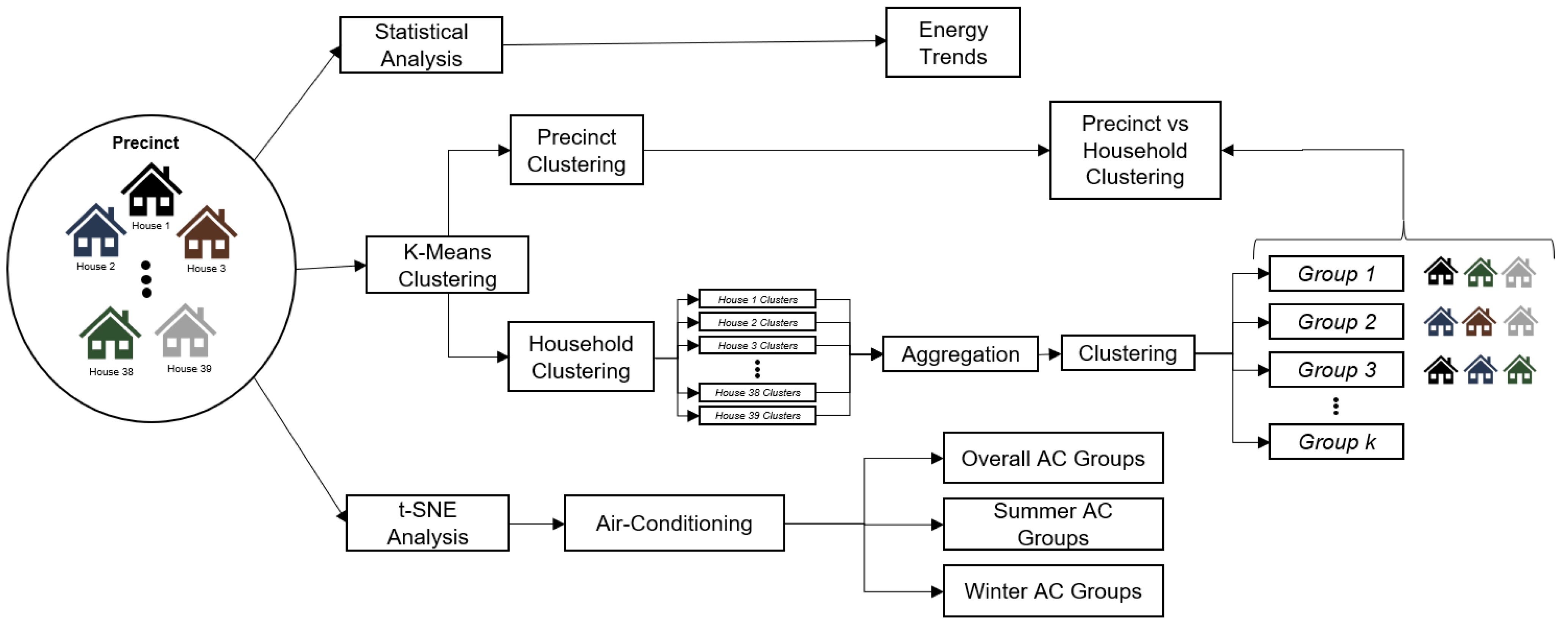
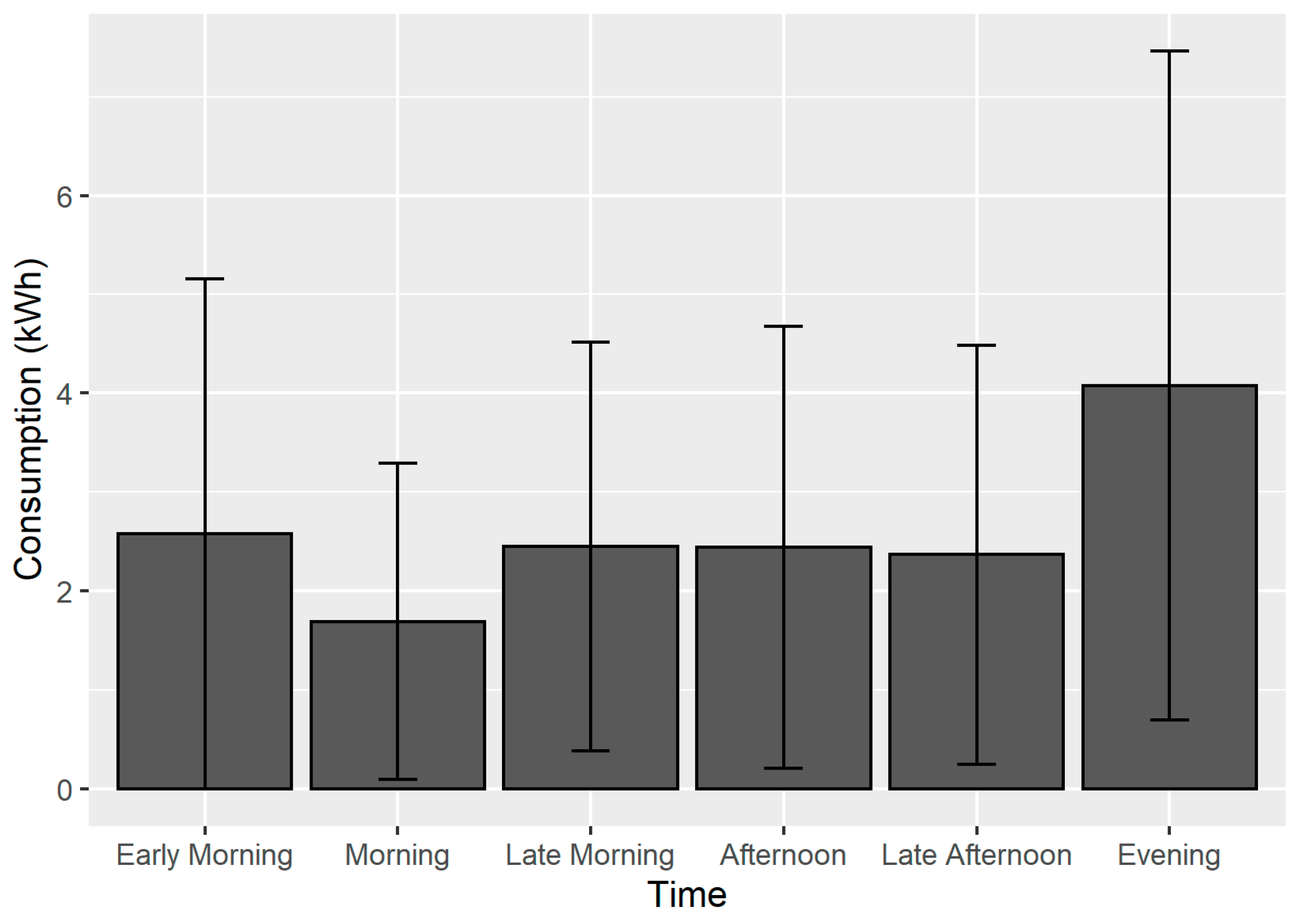
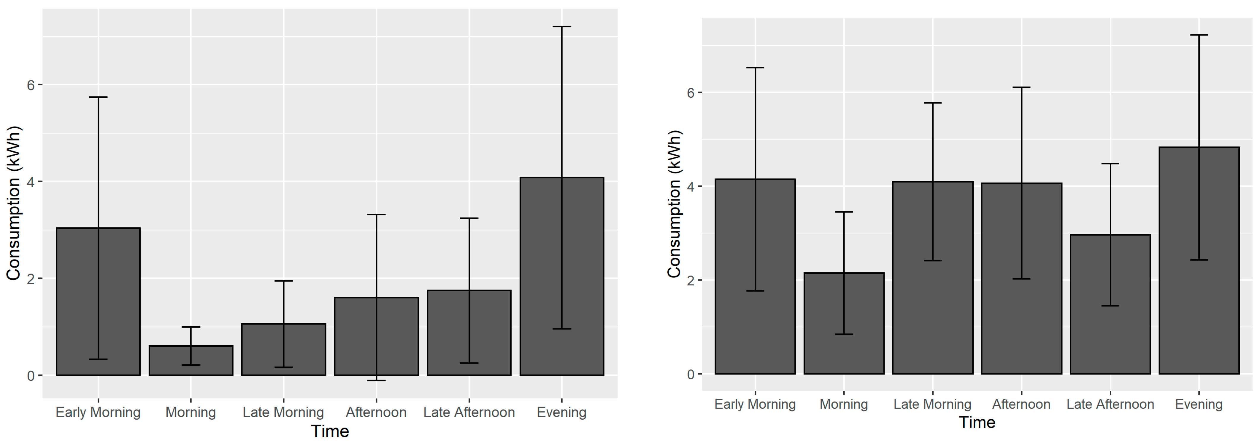
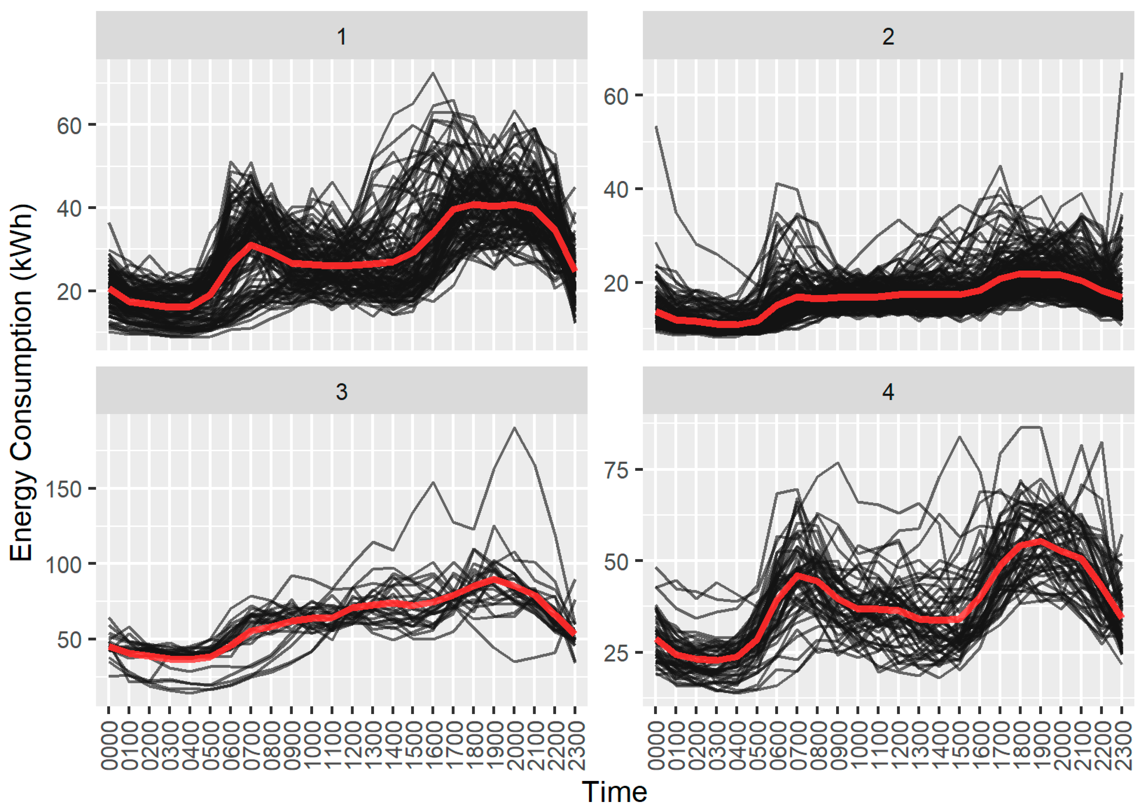
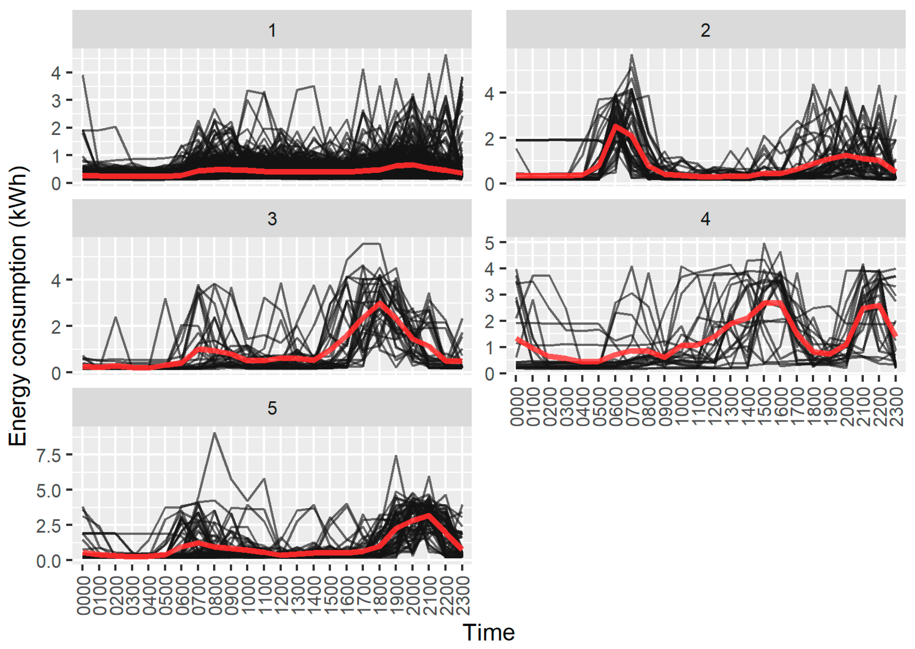
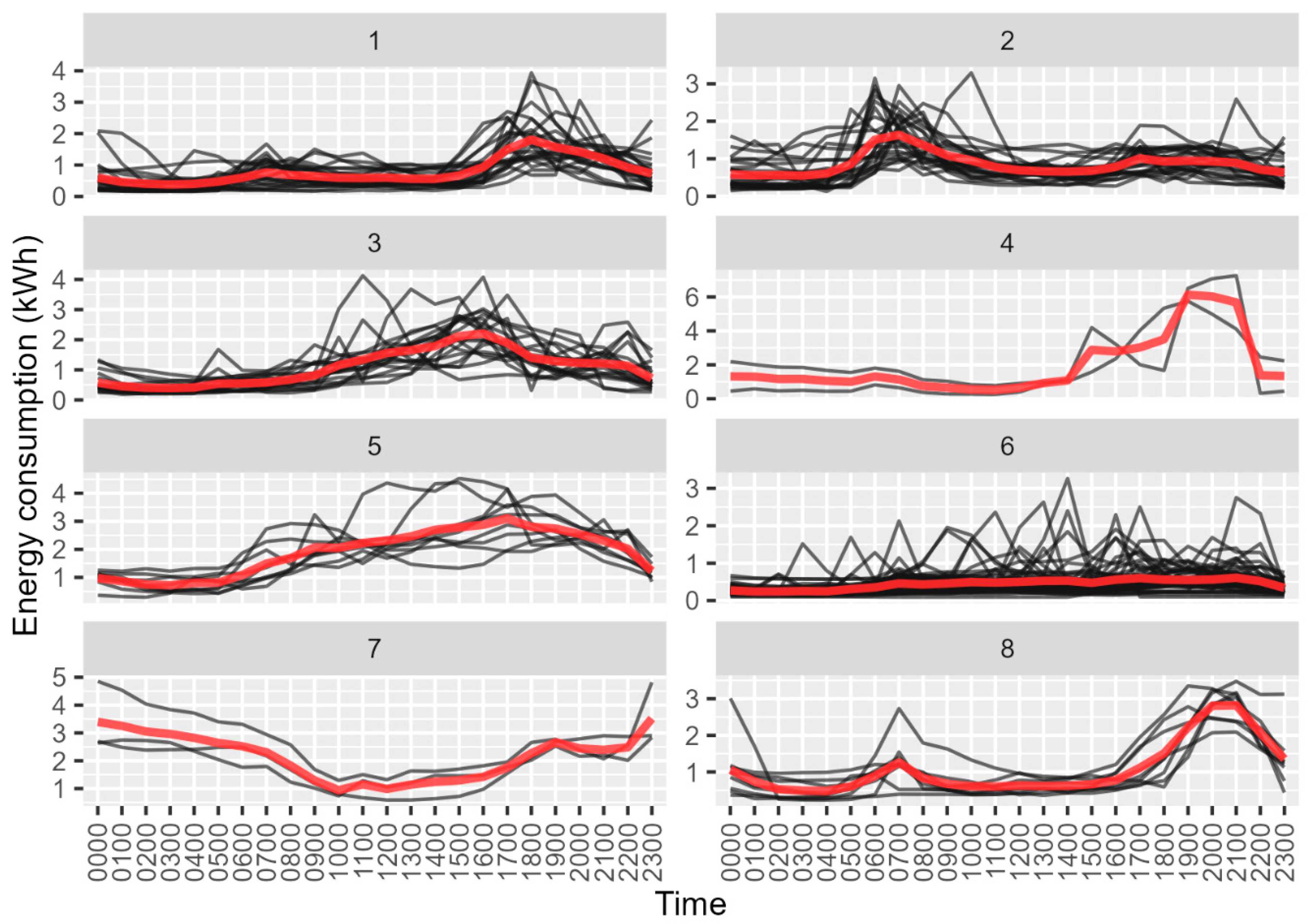
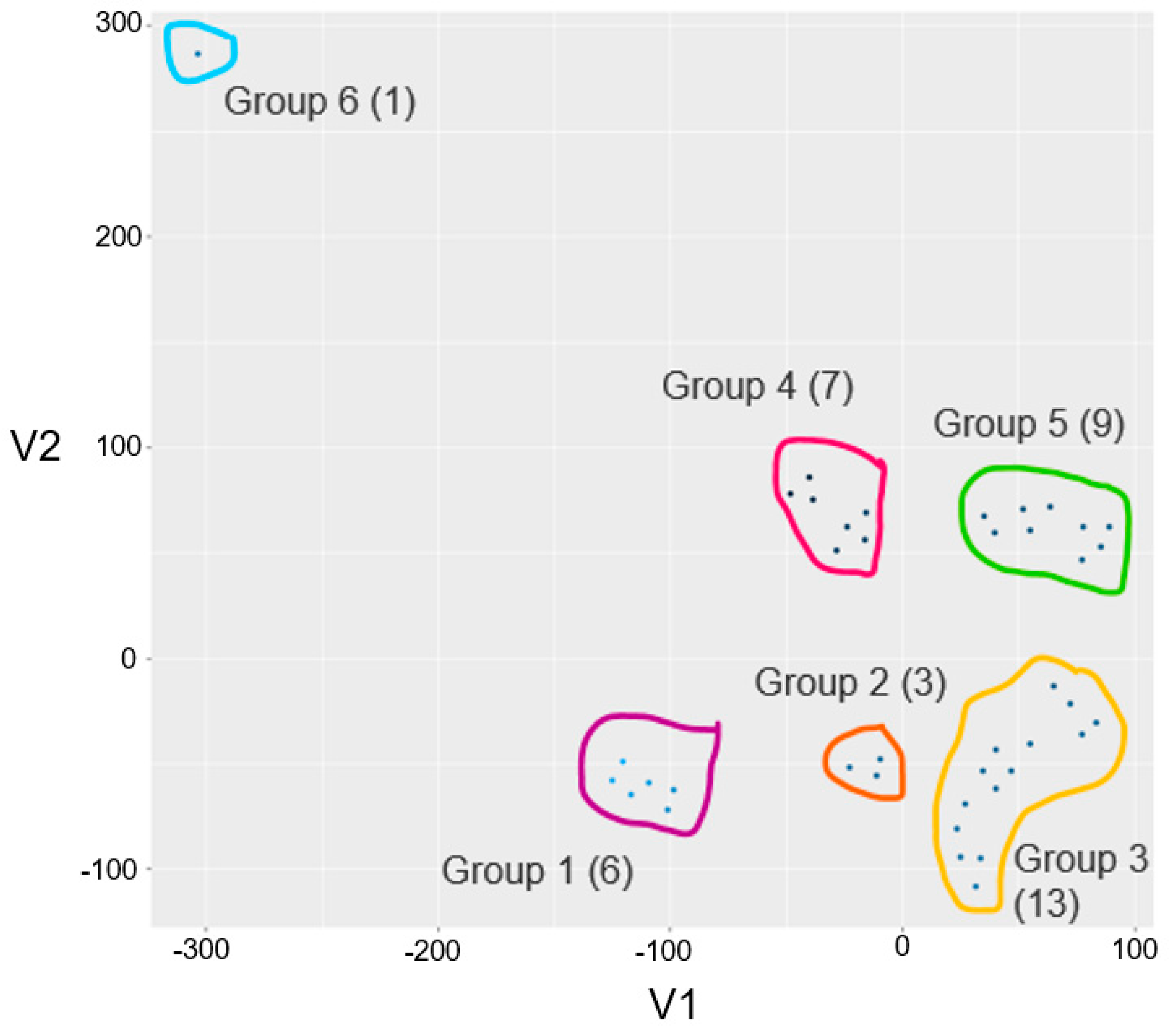
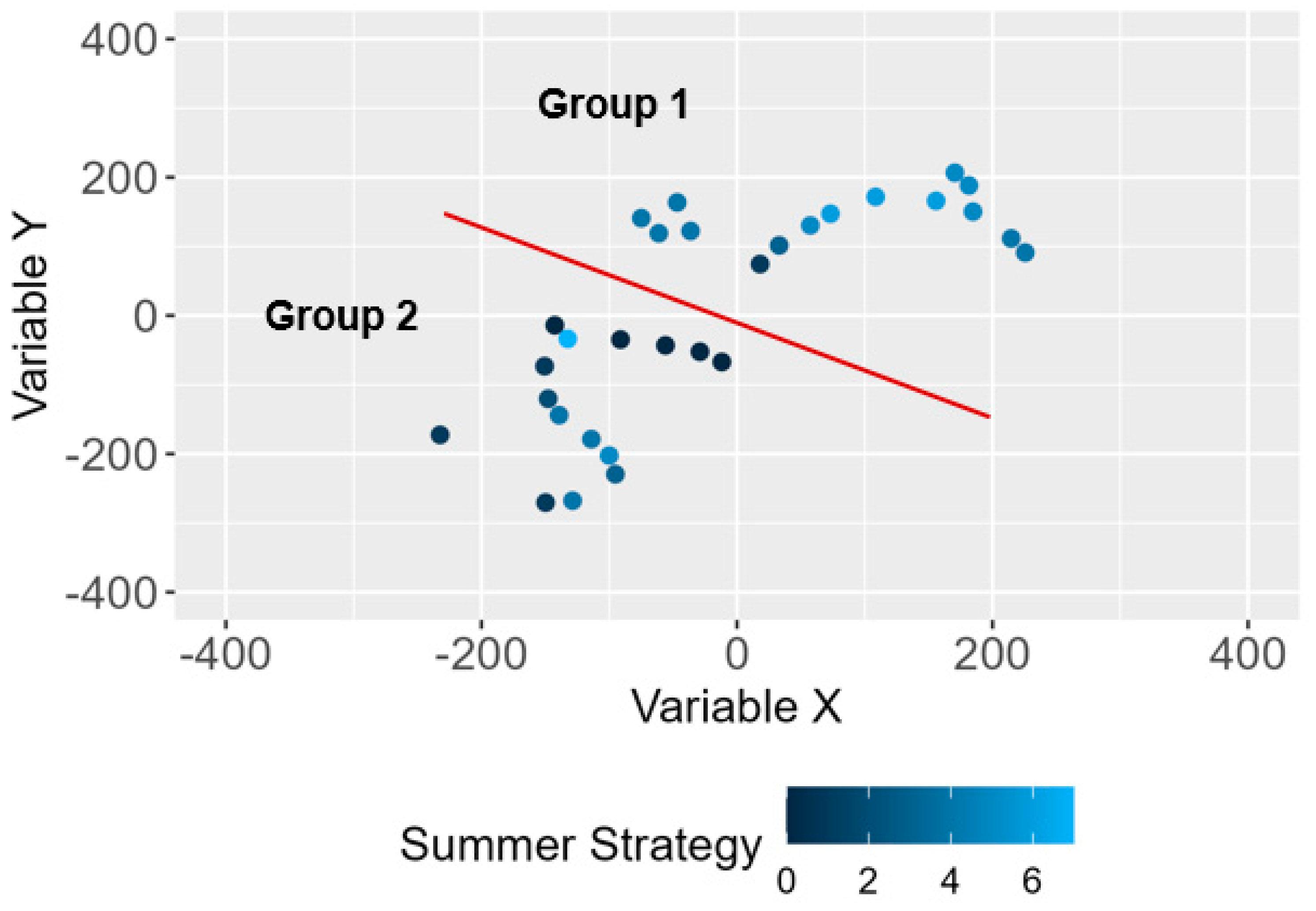
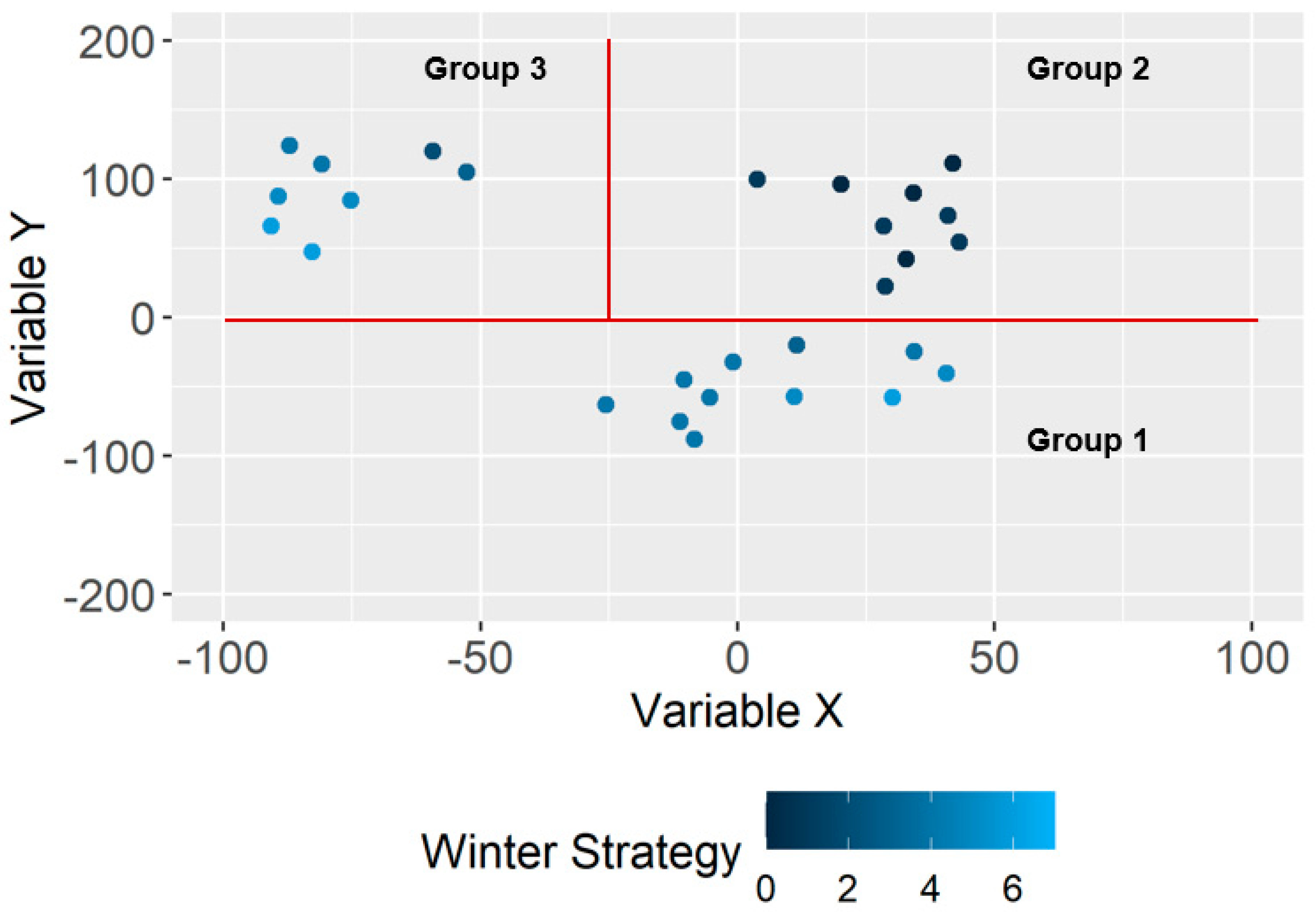
Table 1.
Summary of the energy themes and past work related to this paper.
| Energy Themes | Work Done |
|---|---|
| Social | The social aspect of energy relates to understanding the way energy is consumed within the home and the temporal aspects of this consumption. Past work has focused on developing models and understanding the household practices that result in energy consumption. This has developed the Home System of Practice to understand the household environment and occupants’ routines and lifestyles. |
| Technology | The development of technology and smart energy systems aims to provide a solution for energy supply in this energy transition. Ideally, these systems influence the way energy is consumed through modelling occupant behaviour and predicting their routines and lifestyles. However, these systems are limited in their effectiveness and performance in influencing household energy consumption. |
| Research Gap | This paper explores these two energy themes by evaluating energy behaviours within a precinct and identifying user groupings based on their consumption patterns. These findings are linked to management systems and discuss the importance of human-centric designs that consider the behaviour of the occupants |
Table 2.
Number of clusters identified by the K-means approach for each circuit for each study home.
Table 2.
Number of clusters identified by the K-means approach for each circuit for each study home.
| House ID | Number of Occupants | Mean Daily Consumption (kWh) | Number of Clusters Identified | ||||
|---|---|---|---|---|---|---|---|
| Total Energy Usage | Lights | Oven | Power | AC | |||
| 1 | 1 | 11.5 | 3 | 4 | 15 | 2 | 12 |
| 2 | 2 | 15.8 | 4 | 7 | 8 | 4 | 9 |
| 3 | 3 | 14.1 | 3 | 4 | 7 | 3 | 4 |
| 4 | 3 | 30.6 | 3 | 2 | 11 | 2 | 4 |
| 5 | 5 | 26.5 | 3 | 6 | 11 | 3 | 7 |
| 6 | 4 | 11.8 | 2 | 8 | 10 | 2 | 8 |
| 7 | 3 | 16.9 | 2 | 4 | 15 | 2 | 8 |
| 8 | 3 | 13.9 | 5 | 2 | 7 | 14 | 4 |
| 9 | 4 | 13.8 | 5 | 2 | 11 | 2 | 15 |
| 10 | 2 | 20.9 | 7 | 4 | 14 | 2 | 6 |
| 11 | 3 | 24.4 | 2 | 3 | 15 | 2 | 3 |
| 12 | 4 | 26.7 | 2 | 7 | 15 | 2 | 4 |
| 13 | 2 | 15.9 | 5 | 7 | 12 | 2 | 7 |
| 14 | 5 | 15.4 | 2 | 6 | 11 | 2 | 7 |
| 15 | 4 | 14.0 | 3 | 4 | 12 | 2 | 12 |
| 16 | 3 | 20.1 | 9 | 5 | 7 | 3 | 9 |
| 17 | 1 | 22.3 | 2 | 8 | 11 | 4 | 2 |
| 18 | 3 | 19.7 | 13 | 7 | 10 | 12 | 15 |
| 19 | 1 | 12.1 | 3 | 2 | 5 | 2 | 7 |
| 20 | 4 | 12.5 | 2 | 3 | 15 | 2 | 13 |
| 21 | 3 | 9.8 | 3 | 3 | 11 | 2 | 10 |
| 22 | 2 | 8.7 | 2 | 2 | 2 | 3 | 6 |
| 23 | 5 | 19.5 | 5 | 9 | 11 | 9 | 5 |
| 24 | 3 | 18.3 | 4 | 2 | 14 | 5 | 14 |
| 25 | 4 | 11.7 | 3 | 4 | 15 | 2 | 12 |
| 26 | 4 | 25.8 | 5 | 2 | 15 | 2 | 10 |
| 27 | 1 | 4.5 | 2 | 5 | 4 | 5 | 5 |
| 28 | 3 | 10.6 | 11 | 4 | 15 | 5 | 14 |
| 29 | 3 | 26.0 | 2 | 3 | 11 | 3 | 2 |
| 30 | 1 | 9.1 | 3 | 2 | 13 | 7 | 6 |
| 31 | 2 | 15.4 | 6 | 5 | 13 | 6 | 13 |
| 32 | 2 | 12.5 | 2 | 3 | 7 | 11 | 5 |
| 33 | 3 | 10.9 | 2 | 2 | 15 | 15 | 11 |
| 34 | 3 | 14.7 | 2 | 3 | 9 | 2 | 9 |
| 35 | 3 | 9.7 | 3 | 8 | 13 | 2 | 12 |
| 36 | 4 | 12.8 | 4 | 8 | - | 2 | 8 |
| 37 | 4 | 22.2 | 3 | 4 | 6 | 2 | 7 |
| 38 | 3 | 8.3 | 5 | 13 | 4 | 12 | 6 |
| 39 | 4 | 13.3 | 3 | 2 | 4 | 5 | 7 |
| Mean | 3.8 | 4.6 | 10.6 | 4.3 | 8.2 | ||
| Standard Deviation | 2.5 | 2.6 | 3.8 | 3.7 | 3.7 | ||
Table 3.
Individual FLL homes matched to the eight Household Clusters identified previously. A tick represents that the home follows that Household Cluster, and no tick means that the home did not follow that cluster.
Table 3.
Individual FLL homes matched to the eight Household Clusters identified previously. A tick represents that the home follows that Household Cluster, and no tick means that the home did not follow that cluster.
| House ID | Household Cluster | |||||||
|---|---|---|---|---|---|---|---|---|
| 1 | 2 | 3 | 4 | 5 | 6 | 7 | 8 | |
| 1 | 🗸 | 🗸 | 🗸 | |||||
| 2 | 🗸 | 🗸 | 🗸 | 🗸 | ||||
| 3 | 🗸 | 🗸 | ||||||
| 4 | 🗸 | 🗸 | 🗸 | |||||
| 5 | 🗸 | 🗸 | 🗸 | |||||
| 6 | 🗸 | 🗸 | ||||||
| 7 | 🗸 | 🗸 | ||||||
| 8 | 🗸 | 🗸 | 🗸 | 🗸 | ||||
| 9 | 🗸 | 🗸 | 🗸 | 🗸 | 🗸 | |||
| 10 | 🗸 | 🗸 | 🗸 | 🗸 | 🗸 | 🗸 | ||
| 11 | 🗸 | 🗸 | ||||||
| 12 | 🗸 | 🗸 | ||||||
| 13 | 🗸 | 🗸 | 🗸 | 🗸 | ||||
| 14 | 🗸 | 🗸 | ||||||
| 15 | 🗸 | 🗸 | 🗸 | |||||
| 16 | 🗸 | 🗸 | 🗸 | |||||
| 17 | 🗸 | 🗸 | ||||||
| 18 | 🗸 | 🗸 | ||||||
| 19 | 🗸 | 🗸 | ||||||
| 20 | 🗸 | 🗸 | ||||||
| 21 | 🗸 | 🗸 | 🗸 | |||||
| 22 | 🗸 | 🗸 | ||||||
| 23 | 🗸 | 🗸 | 🗸 | 🗸 | ||||
| 24 | 🗸 | 🗸 | 🗸 | |||||
| 25 | 🗸 | 🗸 | 🗸 | |||||
| 26 | 🗸 | 🗸 | 🗸 | 🗸 | 🗸 | |||
| 27 | 🗸 | |||||||
| 28 | 🗸 | 🗸 | 🗸 | 🗸 | ||||
| 29 | 🗸 | 🗸 | ||||||
| 30 | 🗸 | 🗸 | 🗸 | |||||
| 31 | 🗸 | 🗸 | 🗸 | 🗸 | 🗸 | |||
| 32 | 🗸 | |||||||
| 33 | 🗸 | 🗸 | ||||||
| 34 | 🗸 | 🗸 | ||||||
| 35 | 🗸 | 🗸 | ||||||
| 36 | 🗸 | 🗸 | 🗸 | |||||
| 37 | 🗸 | 🗸 | 🗸 | |||||
| 38 | 🗸 | 🗸 | 🗸 | |||||
| 39 | 🗸 | 🗸 | 🗸 | |||||
Table 4.
Frequency of matches for each household cluster.
| Household Cluster | 1 | 2 | 3 | 4 | 5 | 6 | 7 | 8 |
|---|---|---|---|---|---|---|---|---|
| Number of homes | 22 | 18 | 17 | 2 | 8 | 34 | 3 | 8 |
Table 5.
Number of households allocated to Clusters 1, 2 and 3.
| Subset | Number of Households |
|---|---|
| Cluster 1 only | 8 |
| Cluster 2 only | 6 |
| Cluster 3 only | 3 |
| Clusters 1 and 3 | 6 |
| Clusters 1 and 2 | 4 |
| Clusters 2 and 3 | 4 |
| Clusters 1, 2 and 3 | 4 |
Table 6.
Quantitative and qualitative data for the six groups identified by the t-SNE results.
| Group | House Area (m2) | Energy per Area (Wh/m2) | Summer AC (kWh) | Winter AC (kWh) | Self-Reported Comfort in Summer (scale of 1 to 7) | Self-Reported Comfort in Winter (Scale 1 to 7) |
|---|---|---|---|---|---|---|
| i | 244 | 2 | 0.49 | 0.89 | 6 | 6 |
| ii | 205 | 1.1 | 0.30 | 0.37 | 5 | 5.3 |
| iii | 194 | 0.9 | 0.22 | 0.31 | 4.7 | 4.6 |
| iv | 132 | 1.5 | 0.23 | 0.30 | 5.6 | 5.4 |
| v | 171 | 1.3 | 0.31 | 0.33 | 4.4 | 4.5 |
| vi | 256 | 0.5 | 0.15 | 0.20 | 5.5 | 5 |
Table 7.
Description of the six groups identified by the t-SNE analysis.
| Group | AC | Internal Area | Comfort | Description |
|---|---|---|---|---|
| i | High | Large | Very High | High AC users with a large internal area with occupants report a high thermal comfort rating in the summer and winter. |
| ii | Medium | Large | High | Medium AC users with a large internal area with occupants report a high thermal comfort rating in summer and winter |
| iii | Low | Large | Medium | Low AC users with a large internal area with occupants report a medium thermal comfort rating in summer and winter |
| iv | Low | Small | High | Low AC users with a small internal area with occupants report a high thermal comfort rating in summer and winter |
| v | Medium | Small | Medium | Medium AC user & small house |
| vi | Very Low | Large | High | Very Low AC user & a big house |
Table 8.
Quantitative and qualitative data for the six groups identified for summer AC energy data.
| AC Usage (kWh/m2) | Thermostat Setting (deg C) | Number of Reasons to Use AC Less Frequently | Reliance on AC for Thermal Comfort | Self-Reported Comfort | |
|---|---|---|---|---|---|
| Group 1 | 0.05 | 22.29 | 2.32 | 2.32 | 5.42 |
| Group 2 | 0.04 | 23.21 | 2.75 | 3.58 | 4.25 |
Table 9.
Quantitative and qualitative data for the six groups identified for winter AC energy data.
| AC Usage (kWh/m2) | Thermostat Setting (deg C) | Number of Reasons to Use AC Less Frequently | Reliance on AC for Thermal Comfort | Self-Reported Comfort | |
|---|---|---|---|---|---|
| Group 1 | 0.06 | 23.1 | 2.6 | 4.5 | 4.6 |
| Group 2 | 0.02 | 20.0 | 5.0 | 1.0 | 5.0 |
| Group 3 | 0.05 | 23.8 | 2.0 | 0.8 | 5.4 |
Disclaimer/Publisher’s Note: The statements, opinions and data contained in all publications are solely those of the individual author(s) and contributor(s) and not of MDPI and/or the editor(s). MDPI and/or the editor(s) disclaim responsibility for any injury to people or property resulting from any ideas, methods, instructions or products referred to in the content. |
© 2023 by the authors. Licensee MDPI, Basel, Switzerland. This article is an open access article distributed under the terms and conditions of the Creative Commons Attribution (CC BY) license (https://creativecommons.org/licenses/by/4.0/).
Share and Cite
MDPI and ACS Style
Malatesta, T.; Li, Q.; Breadsell, J.K.; Eon, C. Distinguishing Household Groupings within a Precinct Based on Energy Usage Patterns Using Machine Learning Analysis. Energies 2023, 16, 4119. https://doi.org/10.3390/en16104119
AMA Style
Malatesta T, Li Q, Breadsell JK, Eon C. Distinguishing Household Groupings within a Precinct Based on Energy Usage Patterns Using Machine Learning Analysis. Energies. 2023; 16(10):4119. https://doi.org/10.3390/en16104119
Chicago/Turabian StyleMalatesta, Troy, Qilin Li, Jessica K. Breadsell, and Christine Eon. 2023. "Distinguishing Household Groupings within a Precinct Based on Energy Usage Patterns Using Machine Learning Analysis" Energies 16, no. 10: 4119. https://doi.org/10.3390/en16104119
Note that from the first issue of 2016, this journal uses article numbers instead of page numbers. See further details here.