Probabilistic Decline Curve Analysis: State-of-the-Art Review

Abstract

The decline curve analysis (DCA) technique is the simplest, fastest, least computationally demanding, and least data-required reservoir forecasting method. Assuming that the decline rate of the initial production data will continue in the future, the estimated ultimate recovery (EUR) can be determined at the end of the well/reservoir lifetime based on the declining mode. Many empirical DCA models have been developed to match different types of reservoirs as the decline rate varies from one well/reservoir to another. In addition to the uncertainties related to each DCA model’s performance, structure, and reliability, any of them can be used to estimate one deterministic value of the EUR, which, therefore, might be misleading with a bias of over- and/or under-estimation. To reduce the uncertainties related to the DCA, the EUR could be assumed to be within a certain range, with different levels of confidence. Probabilistic decline curve analysis (pDCA) is the method used to generate these confidence intervals (CIs), and many pDCA approaches have been introduced to reduce the uncertainties that come with the deterministic DCA. The selected probabilistic type of analysis (i.e., frequentist or Bayesian), the used DCA model(s), the type and the number of wells, the sampling technique of the data or the model’s parameters, and the parameters themselves undergo a probability distribution, and these are the main differences among all of these approaches and the factors that determine how each approach can quantify the uncertainties and mitigate them. In this work, the Bayesian and frequentist approaches are deeply discussed. In addition, the uncertainties of DCA are briefly discussed. Further, the bases of the different probabilistic analyses are explained. After that, 15 pDCA approaches are reviewed and summarized, and the differences among them are stated. The study concludes that Bayesian analysis is generally more effective than frequentist analysis, though with narrower CIs. However, the choice of DCA model and sampling algorithm can also affect the bounds of the CIs and the calculation of the EUR. Moreover, the pDCA approach is recommended for quantifying uncertainties in DCA, with narrower CIs that indicate greater effectiveness. However, the computational time and the number of iterations in sampling are also considered critical factors. That is why various assumptions and modifications have been made in the pDCA approaches, including the assumption of a certain probability distribution for the sampled parameters to improve their reliability of reserve estimation. The motivation behind this research was to present a full state-of-the-art review of the pDCA and the latest developments in this area of research.

1. Introduction

Different decline curve analysis (DCA) models have been recently developed and used, especially for unconventional shale reservoirs [1,2]. There are several uncertainties in estimating the ultimate recovery(EUR) using one or more DCA models [3]. To assess the uncertainty in reserve estimations based on DCA, analysts are increasingly using probabilistic techniques because the results are based on a statistical study of historical data, which frequently have a lot of noise [4]. When production profiles show an unknown behavior at a late time during an evaluation of the reservoirs, uncertainty analysis is extremely important. Hence, it is essential to predict production using a probabilistic methodology [5].

The challenge in estimating probabilistic reserves using DCA is not only in determining how to identify the probabilistic features of complicated production data sets but also in determining which approach (i.e., set of steps) should be followed to improve the reliability of the uncertainty quantification and forecasting of the reserve with a higher level of confidence.

In this paper, the bases of the probabilistic analysis are firstly introduced. Secondly, the main sources of uncertainties related to production forecasting using empirical methods are summarized. In addition, the combined DCA models in the previous studies are presented. After that, 15 pDCA approaches are comprehensively reviewed and compared. The goal of this research was to highlight the key distinctions between the pDCA techniques, as well as their difficulties, constraints, and dependability.

1.1. Overview of DCA Models

DCA, as a tool to estimate reserves in oil and gas wells/reservoirs, was firstly introduced by Arps [6]. Three models were proposed to describe the production decline of a conventional well (exponential, harmonic, and hyperbolic). The three main assumptions related to Arps’s models are: (1) the flow has reached the boundary (i.e., boundary-dominated flow (BDF)), (2) there are stable producing conditions over a certain period, and (3) there are stable reservoir conditions [7]. The three models are distinguished based on the value of the decline curve exponent b (Table 1). Several models were developed for DCA after Arps’ models [1]. The reason was mainly that Arps’s models are not effective for unconventional reservoirs [3,8,9], and the EUR is overestimated with a b-value of greater than one [10].

In unconventional oil and gas wells, the production mode is described by a fast decline in the flow rate in the early time and a long tail of a very slow decline in the late time [11,12]. The main reasons for this are the system complexity and the developing methodology of such reservoirs [13]. These reservoirs are developed by drilling a horizontal well with multistage hydraulic fractures [14]. The hydraulic fractures create artificial permeability, allowing flow to the wellbore [14,15]. The flow is transient in these fractures and could last for a long time before reaching the BDF [16,17,18]. To match the production behavior of unconventional reservoirs, many DCA models have been developed [19]. Table 1 shows several DCA models, such as Arps’s models, modified Arps’s model, the logistic growth model (LGM), the stretched exponential production decline (SEPD) model, Duong’s model, the extended exponential decline curve analysis (EEDCA) model, Pan’s model, and the power law exponential (PLE) model. Different DCA models were developed to predict future performance of both conventional and unconventional reservoirs [20]. These DCA models (Table 1) are coupled with various pDCA methods to estimate reliable EUR.

Table 1. Summary of the DCA models combined with the pDCA approaches.

Model	(q) versus (t) *	Reference
Exponential Arps (1945)	$q_t=q_i\exp \left(-D_{i}t\right)$	[6]
Hyperbolic Arps (1945)	$q_t=\frac{q_i}{{\left(1+{bD}_{i}t\right)}^{1/b}}$	[6]
Harmonic Arps (1945)	$q_t=\frac{q_i}{\left(1+D_{i}t\right)}$	[6]
Modified Arps approach (2008)	$q_t=\frac{{\left(q_i\right)}_{\Delta t=0}}{{\left[1+b{\left(D_i\right)}_{\Delta t=0}\left(t-t_{\mathrm{Last} }\right)\right]}^{1/b}}$	[21,22]
$$\begin{gathered} \mathrm{PLE} \left(2008\right) \\ {D}_{\mathrm{\infty }}\ne 0 \\ {D}_{\mathrm{\infty }}=0 \end{gathered}$$	$q=q_{\mathrm{i}}.e^{\left[-D_{\mathrm{\infty }}t-D_i{t}^n\right]}$ $q=q_{\mathrm{i}}.e^{\left[-D_i{t}^n\right]}$	[23,24]
SEPD (2010)	$q=q_i\cdot \mathrm{e}\mathrm{x}\mathrm{p}\left[-(t/\tau {)}^{n_{\mathrm{SEPD} }}\right]$	[25,26]
Duong (2010, 2011)	$q=q_{\mathrm{i}}\cdot t^{-m_{\mathrm{D}}}\mathrm{e}\mathrm{x}\mathrm{p}\left[\frac{a_{\mathrm{D}}}{1-m_{\mathrm{D}}}\left(t^{1-m_{\mathrm{D}}}-1\right)\right]$	[27,28]
LGM (2011)	$q=q_{\mathrm{i}}\cdot \frac{n_{\mathrm{LGM} }-a_{\mathrm{LGM} }\cdot t^{n_{LGM}-1}}{{\left(a_{\mathrm{LGM} }+t^{n_{LGM}}\right)}^2}$	[29]
EEDCA (2015)	$q=q_i\cdot \mathrm{e}\mathrm{x}\mathrm{p}\left[-\left({\beta }_1+{\beta }_e\cdot e^{-t^{n_E}}\right)t\right]$	[30]
Pan (2017)	$q_t=\Delta P\left(\frac{\beta }{\sqrt{t}}+J_{\mathrm{\infty }}\right)e^{-\left(2\beta \sqrt{t}+J_{\mathrm{\infty }}t\right)/\left(c_t{V}_p\right)}$	[31]

* Letters with the subscript of the model’s initials are the fitting parameters.

Table 1. Summary of the DCA models combined with the pDCA approaches.

Model	(q) versus (t) *	Reference
Exponential Arps (1945)	$q_t=q_i\exp \left(-D_{i}t\right)$	[6]
Hyperbolic Arps (1945)	$q_t=\frac{q_i}{{\left(1+{bD}_{i}t\right)}^{1/b}}$	[6]
Harmonic Arps (1945)	$q_t=\frac{q_i}{\left(1+D_{i}t\right)}$	[6]
Modified Arps approach (2008)	$q_t=\frac{{\left(q_i\right)}_{\Delta t=0}}{{\left[1+b{\left(D_i\right)}_{\Delta t=0}\left(t-t_{\mathrm{Last} }\right)\right]}^{1/b}}$	[21,22]
$$\begin{gathered} \mathrm{PLE} \left(2008\right) \\ {D}_{\mathrm{\infty }}\ne 0 \\ {D}_{\mathrm{\infty }}=0 \end{gathered}$$	$q=q_{\mathrm{i}}.e^{\left[-D_{\mathrm{\infty }}t-D_i{t}^n\right]}$ $q=q_{\mathrm{i}}.e^{\left[-D_i{t}^n\right]}$	[23,24]
SEPD (2010)	$q=q_i\cdot \mathrm{e}\mathrm{x}\mathrm{p}\left[-(t/\tau {)}^{n_{\mathrm{SEPD} }}\right]$	[25,26]
Duong (2010, 2011)	$q=q_{\mathrm{i}}\cdot t^{-m_{\mathrm{D}}}\mathrm{e}\mathrm{x}\mathrm{p}\left[\frac{a_{\mathrm{D}}}{1-m_{\mathrm{D}}}\left(t^{1-m_{\mathrm{D}}}-1\right)\right]$	[27,28]
LGM (2011)	$q=q_{\mathrm{i}}\cdot \frac{n_{\mathrm{LGM} }-a_{\mathrm{LGM} }\cdot t^{n_{LGM}-1}}{{\left(a_{\mathrm{LGM} }+t^{n_{LGM}}\right)}^2}$	[29]
EEDCA (2015)	$q=q_i\cdot \mathrm{e}\mathrm{x}\mathrm{p}\left[-\left({\beta }_1+{\beta }_e\cdot e^{-t^{n_E}}\right)t\right]$	[30]
Pan (2017)	$q_t=\Delta P\left(\frac{\beta }{\sqrt{t}}+J_{\mathrm{\infty }}\right)e^{-\left(2\beta \sqrt{t}+J_{\mathrm{\infty }}t\right)/\left(c_t{V}_p\right)}$	[31]

* Letters with the subscript of the model’s initials are the fitting parameters.

1.2. Uncertainties Related to DCA

The EUR estimated from any DCA model is a deterministic value that might be over- and/or under-estimated according to the used model [32]. The amount of data available for fitting and defining the model’s parameters, the regression technique itself utilized for fitting, the quality of the data, and the outlier detection and removal strategies used to improve the quality of the data are all potential sources of uncertainty. Some DCA models are more sensitive to the quantity and quality of production data while others are more sensitive to both. These variations change depending on the model [33]. Each mentioned source of uncertainty subjected to DCA models should be separately investigated and quantified. This investigation is out of the scope of this research, however, and as an example, Figure 1 shows that different regression techniques can introduce uncertainty into the estimation of the EUR, despite using the same DCA model, the same portion of the fitting data set, and the same portion of the prediction data set for analysis [34].

It should be pointed out that a reliable EUR is more affected by the performance of the selected DCA itself. In other words, if a DCA model tends to overestimate the reserve, the EUR that could be obtained from any pDCA will still be overestimated, and vice versa. The only difference is that the DCA model provides a deterministic value of the EUR while the pDCA approach provides a range of EUR values. In our previous research, we comprehensively reviewed numerous DCA models and their performances in overestimating or underestimating the EUR [35]. Moreover, other studies have addressed the conditions of applying an effective DCA [36,37].

1.3. Probabilistic DCA (pDCA)

With pDCA, probabilities are introduced for any estimated value based on the degree of uncertainty. Unlike DCA models, pDCA approaches consider talking with probability language rather than with deterministic values [38]. pDCA approaches usually estimate the reserves with three levels of confidence (P10, P50, and P90) and a corresponding 80% confidence interval (CI). The question is, how accurate is this 80% CI? In other words, is the real worth of reserves included within this range 80% of the time based on a substantial body of analyses? The genuine reserve will be outside of 80% confidence ranges of more than 20% if the uncertainties are undervalued, which is frequently the case. These three levels of confidence can be determined using Equations (1)–(3) [39]:

$$P_{10}={\int }_0^{0.90} \frac{1}{(x.\sigma \sqrt{2\pi })}\mathrm{e}\mathrm{x}\mathrm{p}\left(\frac{-(\mathrm{l}\mathrm{n}x-\mu {)}^2}{2{\sigma }^2}\right),$$

(1)

$$P_{50}={\int }_0^{0.50} \frac{1}{(x.\sigma \sqrt{2\pi })}\mathrm{e}\mathrm{x}\mathrm{p}\left(\frac{-(\mathrm{l}\mathrm{n}x-\mu {)}^2}{2{\sigma }^2}\right), \mathrm{a}\mathrm{n}\mathrm{d}$$

(2)

$$P_{90}={\int }_0^{0.10} \frac{1}{(x.\sigma \sqrt{2\pi })}\mathrm{e}\mathrm{x}\mathrm{p}\left(\frac{-(\mathrm{l}\mathrm{n}x-\mu {)}^2}{2{\sigma }^2}\right),$$

(3)

where x is the sample value, μ is the mean, and σ is the standard deviation of the parameter under study.

Usually, P₁₀, P₅₀, and P₉₀ represent these three levels of uncertainties. P₁₀ is the optimistic case, P₅₀ is the moderate case, and P₉₀ is the pessimistic case. In other words, P₁₀ and P₉₀ represent the limits that the true EUR might be located within. The CI between those limits is crucial as the narrower the CI, the less uncertainty we have [40].

1.4. Types of Statistical Analysis

Frequentist and Bayesian are the two main statistical analyses related to probabilistic studies. A frequentist analysis is only driven by the data, but a Bayesian analysis takes into account prior information (background knowledge) [41]. The frequentist technique evaluates the likelihood of finding another data set at least as extreme as the one gathered, whereas the Bayesian approach calculates the likelihood that a certain hypothesis will be true, given the p-value that is updated with more data [42,43].

The prior distribution (simply prior) of the outcome θ is labeled as P(θ). It is the probability distribution that reflects what is known about an outcome before a test or other piece of information is acquired. Priors may have little to no background data if they are unavailable or of questionable reliability. These priors are called non-informative. The prior of any parameter is assumed to follow a certain probability distribution. Many probability distributions could be assumed [44].

Uniform distribution is the most common assumption. Given particular parameter values, the likelihood function reflects the assumed distribution of the data. The likelihood function comprises all of the information regarding parameter values collected from the data and how the data affect the posterior distribution [45]. A Bayesian model can only be fully characterized when both the prior distribution and the likelihood function are completely described. The prior distributions and the observed data are combined to create the posterior distribution [46]. It takes into account the most recent knowledge of the parameter values and entails balancing prior knowledge against observed data. Depending on the observed data, it expresses the remaining uncertainty about the set of parameters in question [38].

After taking into consideration the uncertainty of the parameter value that is indicated in the posterior distribution, the posterior predictive distribution indicates the distribution of upcoming, further observations that are collected from the population. It may be calculated via compositional sampling, where fresh observations are generated by drawing parameters from the posterior and adding them to the likelihood function. Equation (4) represents Bayes’ Theorem, by which the most recent understanding of a parameter or hypothesis may be updated when new data become available [47].

$$p(\theta \mid Data)=\frac{p(\mathrm{Data} \mid \theta )\cdot p\left(\theta \right)}{p\left(Data\right)},$$

(4)

where Data refers to the set of observations in the data and θ is a set of the parameters in the model. $p(\theta \mid Data)$ represents the posterior distribution of the parameters, p(Data ∣ θ) is the likelihood function, p(θ) is the prior distribution of the parameters, and p(Data) is the marginal likelihood function (i.e., a normalizing constant).

One of the main distinctions between frequentist and Bayesian inference is the prior; in frequentist studies, findings are purely based on the data that are collected [48]. The previous knowledge might be created using historical information, expert opinions, or a combination of both. When compared to the frequentist technique, which is frequently misinterpreted, the interpretation of results is more intuitive when using a Bayesian approach as considering good prior information can lead to improved predictions. Both the frequentist and Bayesian techniques are effective for data analysis as long as they are appropriately interpreted.

1.5. Resampling Techniques

To perform a probabilistic study, the possible outcomes of uncertain parameters must be estimated. This requires multiple samples to simulate and consider a wide range of possibilities of the important variables. In the case where a single data set is available, multiple data sets are generated by resampling the original data set [49]. Monte Carlo (MC) and Markov Chain Monte Carlo (MCMC) simulations are mathematical techniques used to predict the probability of a variety of outcomes. Unlike MC sampling methods that can draw independent samples from the distribution, the MCMC methods draw dependent samples.

Many sampling algorithms can be coupled with each technique to generate a large number of simulated samples. “A sampling algorithm is said to be enumerative if all the possible samples must be listed to select the random sample and an efficient sampling algorithm is—by definition -the fast one” [50]. Each sampling algorithm has different characteristics.

Table 2. Summary of the resampling techniques combined with the pDCA approaches.

Simulation Technique	Types of Statistic Analysis	Sampling Algorithms
MC	Frequentist	Bootstrap Time series
	Bayesian	Prior sampling
MCMC	Bayesian	Posterior sampling
		Likelihood-based	Nonlikelihood-based
		Metropolis Hasting (MH) Gibbs	Approximate Bayesian computation (ABC)

summarizes the algorithms that are coupled with the MC or MCMC simulation techniques for the different pDCA approaches being addressed in this study. It should be mentioned that the sampling process is the main intensive mathematical computation in the pDCA. Generally, it has been recommended by many recent studies to depend on current computing capabilities, data structures, and management workflows for fast and cost-effective data analysis [51,52,53].

2. pDCA Approaches

pDCA is one of the analysis tools used to quantify and reduce uncertainties. However, the basis of analysis also carries uncertainties. Those uncertainties are mainly related to the assumptions of the probability distributions of the parameters, the sampling techniques, and the computational time. All of these reasons and more have led to the development of several pDCA approaches to make it more effective in predicting the production and narrowing the bounds of P₁₀, P₅₀, and P₉₀.

As mentioned earlier, pDCA is based on providing probability distributions of the parameters of a selected DCA model(s). Here, some questions should be asked, such as: Which model or a combination of models should be used? What was the used sampling technique? What is the type of probability distribution to be assumed that the model’s parameter/s are following? What is/are the parameter(s) to be probability distributed? The different answers to and preferences of these questions have led to the development of many pDCA approaches.

2.1. Jochen’s Approach (1996) [54]

Jochen and Spivey introduced the bootstrap sampling technique, which is related to DCA models [54]. The motivation behind this work was the reason for building the probability levels of interest (i.e., P₁₀, P₅₀, and P₉₀) based on the deterministic results. The simple assumption that the model’s parameters are following a certain distribution is not efficient and easily could be wrong. The authors showed that the unreliability related to such pDCA approaches was due to the use of the same original data to create a probability distribution of the estimator’s (i.e., the selected DCA model’s) parameters. Therefore, the bootstrap technique was used to resample the original data several times and the MC simulation was used to create the probability distribution and estimate P₁₀, P₅₀, and P₉₀. Moreover, they proved that if the number of iterations is larger than 100, the trend will be the same.

Although this method does not require previous knowledge about the prior distributions of the parameters, it assumes that there is no relation between the original data (i.e., independent) and it follows the same distribution, which is wrong as the production data points are, somehow, correlated, and therefore, they are considered a time-series-data structure. Moreover, creating several synthetic data sets from the original production data make this approach computationally intensive, as was reported in their studies.

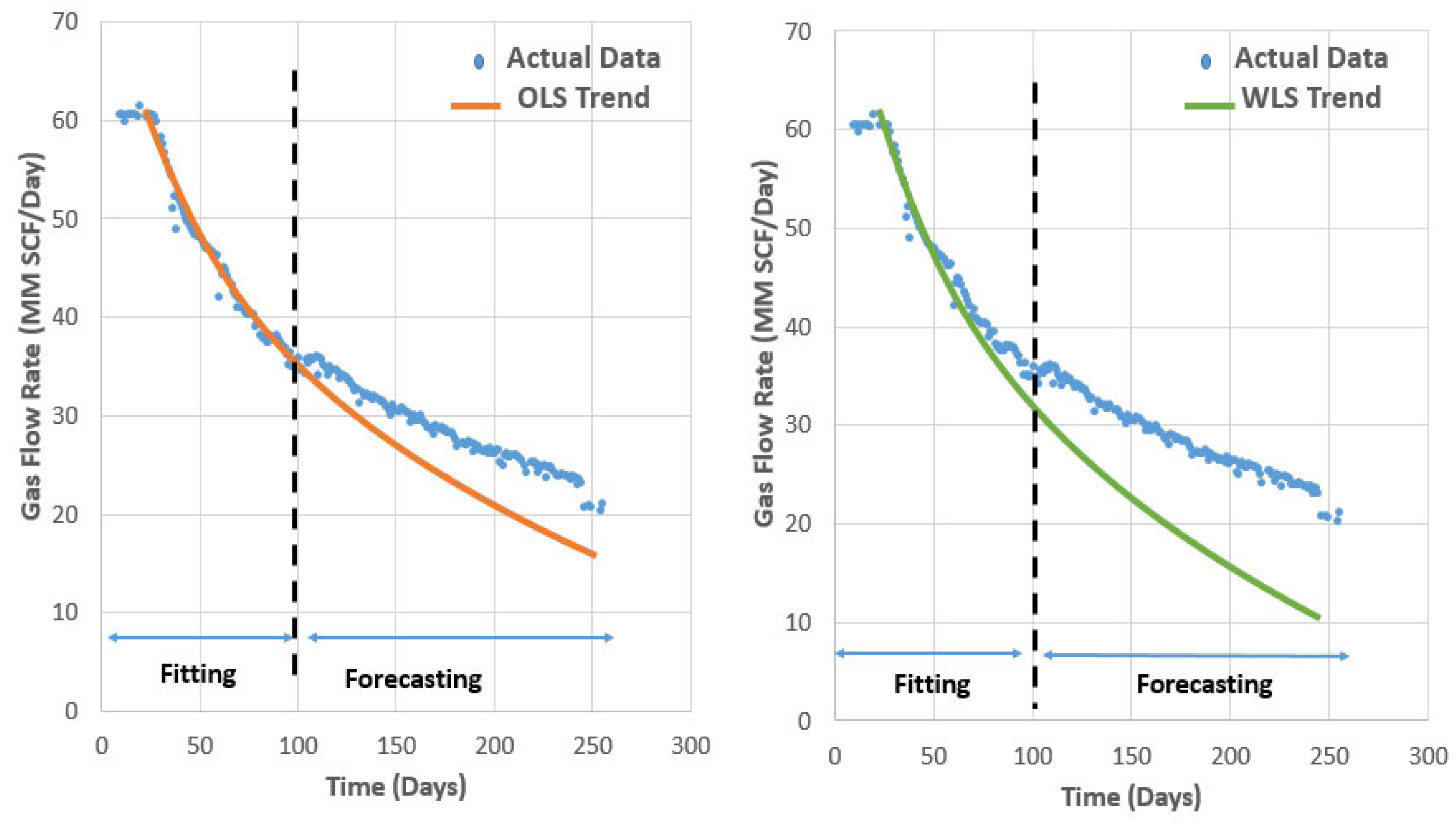
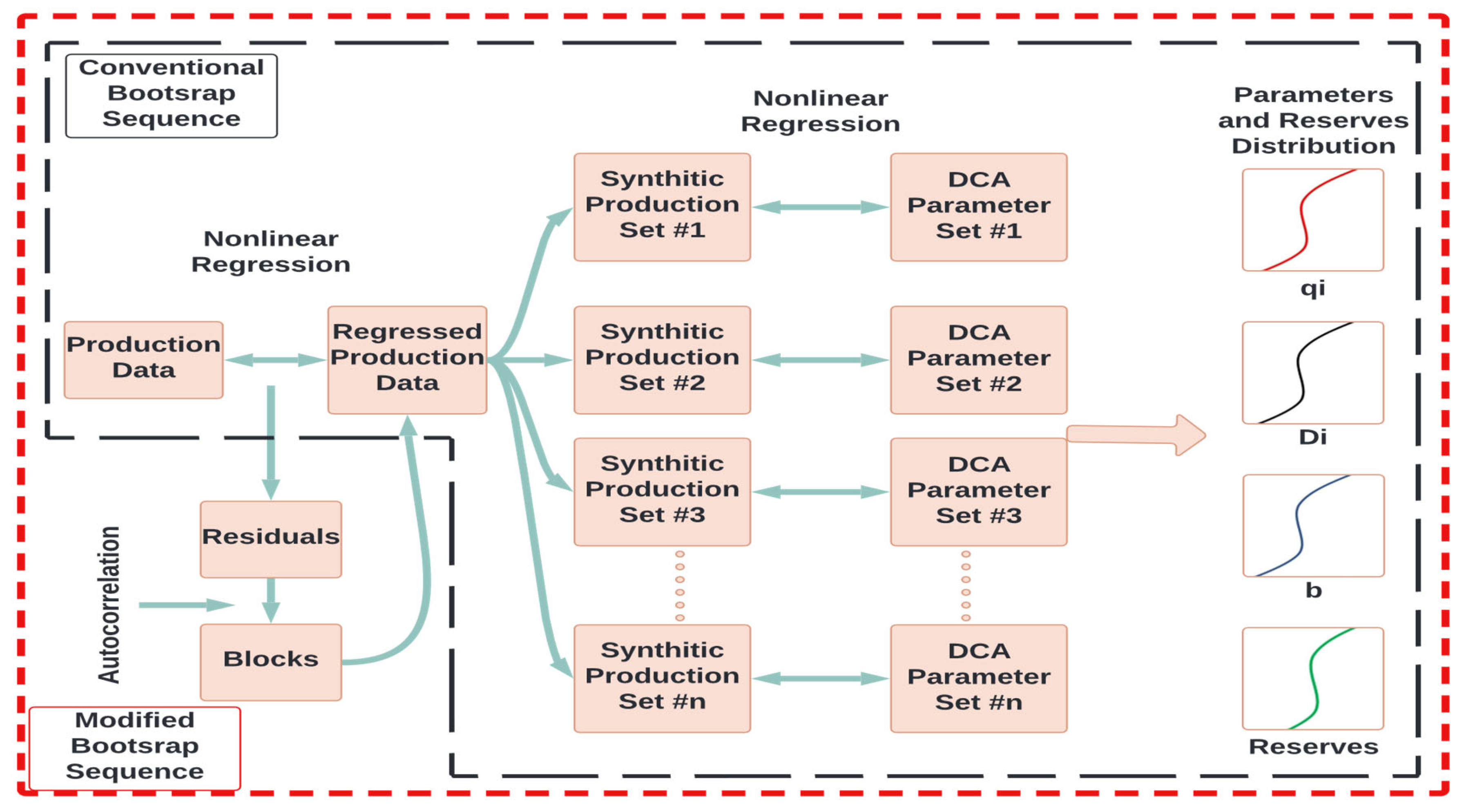
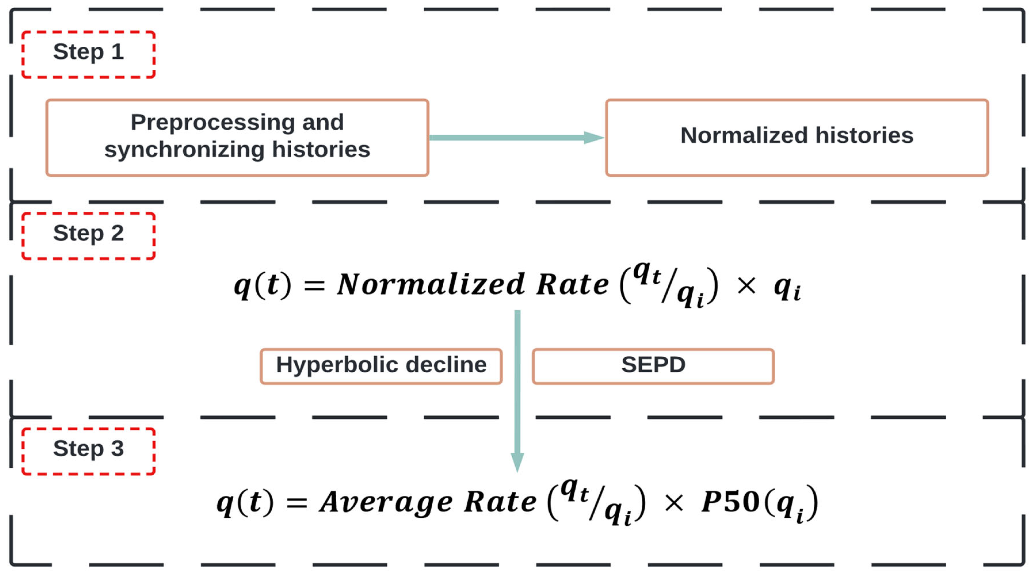
2.2. Cheng’s Approach (2010) [55]

To preserve the data structure, two more steps were added to mitigate the assumptions of the Jochen approach, where Cheng et al. introduced what they called the modified bootstrap method (MBM) [55]. The first step was to perform a nonlinear regression with a hyperbolic or exponential model to fit the production data, and the second step was to use a block resampling of the autocorrelated residuals obtained from the fitted DCA model (Arps, in this case) to the actual data. In the end, the regressed production data are then sampled several times to create synthetic data sets and the accuracy of MBM is dependent on the block size, as denoted by the authors.

Table 3. The differences between Jochen’s and Cheng’s approaches.

Jochen’s Approach	Cheng’s Approach
Uses bootstrap as a sampling technique
Uses Arps’ models as the DCA model
Assumes no correlation between the data points	Assumes a time-series-data structure
Resampled the original data	Resampled the fitted data obtained from a DCA model (Arps)
Random samples from the original data are generated	Samples are generated based on autocorrelated residual blocks

states the differences between Jochen’s and Cheng’s approaches while Figure 2 shows Cheng’s approach modifications to the bootstrap sequence.

In testing Cheng’s approach on 100 oil and gas wells, the coverage range (CR) was improved to 83% compared to the original approach by Jochen (34%). It was suggested that reusing this approach after fitting the recent production history will lead to improving the CR of future production within an 80% CI, as shown in Figure 3. This is called a backward scenario. Conventionally, when all of the production history is used for regression, the actual performance becomes outside of the 80% CI. On the other hand, when only the recent production history is used for regression, the actual performance is within the 80% CI.

Although the MBM has proven to be well-calibrated in unconventional reservoirs [56], it could be inferred that the efficiency of the forecasting decreases for the far future because the interval width becomes wider.

2.3. Minin’s Approach (2011) [57]

The Arps relationship was utilized to analyze 150 horizontal and hydraulically fractured shale gas wells using the pDCA approach and the conventional MC sampling method [57]. A probability distribution was created for the initial decline rate (D_i), decline exponent (b), initial flow rate (q_i), and the initial flow rate divided by the lateral length of the wells (q_i, n). Additionally, they estimated the cumulative distribution functions (CDFs) for each parameter four times (i.e., one CDF after each year of production). They concluded that with time, the b-exponent tended to decrease and stabilize, and D_i tended to increase and stabilize. This is because the flow regime is shifted with time from transient to BDF. Moreover, an incensement of the q_i could be related to the incensement of the lateral horizontal length in the case of drilling a new development well. In addition, there could be a negative correlation between q_i and the horizontal length after reaching a certain length.

The novelty of this work was the conducted pDCA to quantify the uncertainty, and to characterize the flow regime changes with time. It was also used to recommend a drilling design in the case of further development of wells.

2.4. Gong’s Approach (2011) [56]

DCA based on Bayesian statistics was first introduced by Gong [56]. The MCMC sampling technique based on the MH algorithm was used to obtain the posterior distribution of the Arps parameters.

The approach was tested based on 197 shale gas wells. There were two main advantages were related to this work: (1) compared to the MBM method, this approach was 10 times faster, and (2) unlike using the MBM method, the CI did not diverge too much in forecasting the far future. Figure 4 shows a comparison between Gong’s approach and the MBM approach when both approaches are applied to the same dataset.

2.5. Brito’s Approach (2012) [58]

Working on multiple wells rather than a single well, Brito introduced an approach based on a normalized rate called production decline envelopes (PDE) [58]. This approach allowed for analyzing multiple wells and creating decline bands that could be used as the pDCA. This approach can be summarized in three steps, as shown in Figure 5.

The maximum, average, and minimum decline curves can be seen as P₁₀, P₅₀, and P₉₀. The probability distribution is conducted to the initial flow rate and not to the selected DCA model parameters.

2.6. Gonzalez’s Approach (2012) [5]

Following the same steps proposed by Gong et al. (i.e., using the MCMC sampling technique and even the same data), Gonzalez et al. extended this work to be combined with more than one DCA model [5,59]. They used the Arps, modified Arps, Duong’s, PLE, and SEPD models with the MCMC sampling technique. They denoted that P₅₀ using Arps was the best amongst all of them, with the exception of the short production data, while PLE came second and performed well using the short production data. Overall, the estimated P₅₀ from any model was more reliable than each single deterministic reserve value. This work suggested that many DCA models can be combined with the MCMC technique. Comparing all of them can help in minimizing uncertainty about forecasting.

2.7. Fanchi’s Approach (2013) [60]

Fanchi introduced a simple approach to conduct a pDCA-based approach on any selected deterministic model [60]. Working on 110 shale gas wells from different fields and using the Arps and SEPD models, the authors proposed the steps of the approach shown in Figure 6. The MC simulation sampling technique was used to create a probability distribution of the chosen model’s parameters through 1000 iterations after selecting a certain probability distribution for them.

It should be pointed out that the study did not compare the results of the two proposed pDCA studies, and it did not present the coverage range of both of them. Therefore, it could not be considered a comparative analysis.

2.8. Kim’s Approach (2014) [61]

Appling both approaches introduced by Brito and Fanchi, but with small differences, Kim used the MC simulation sampling technique with 5000 iterations and a triangle probability distribution for a single well analysis based on the Arps and SEPD models (similar to Fanchi). Moreover, the PDE was applied for multiple-wells analysis, similar to Brito’s approach [61]. Compared to the previous works of Brito and Fanchi, Kim’s work introduced nothing new, but it used a triangle probability distribution instead of the uniform distribution followed by Fanchi. In addition, Kim performed 5000 iterations while Fanchi performed 1000 iterations.

2.9. Zhukovsky Approach (2016) [62]

Zhukovsky et al. worked on more than 200 shale oil wells [62]. The EUR was estimated using the EEDCA model. The authors used the MCMC simulation as the sampling technique with 100,000 iterations to estimate the posterior probability distribution of the EUR using Matlab software. Calculating P₁₀, P₅₀, and P₉₀ from the CDF, they found that the coverage rate of the 80% CI was 78.4% of the used DCA models, which was a good result. However, many wells showed high average relative errors and average absolute errors related to the actual EUR. They assigned these errors to the low quality of the data collected and being tested and not to the approach itself. Even if the resampling algorithms and different approaches could reduce some of these errors, the heavy noise and fluctuating data could lead to unreliable estimations.

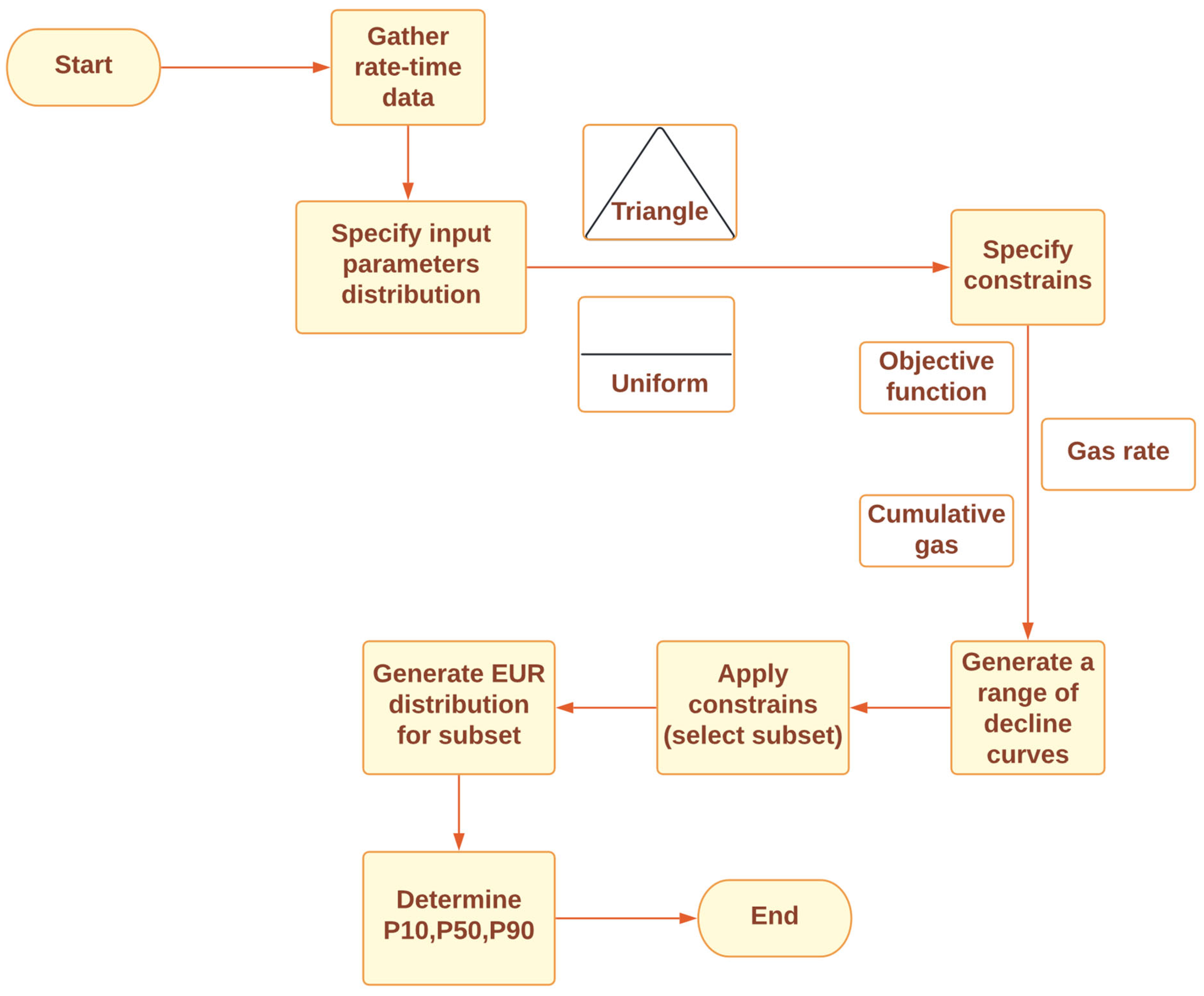
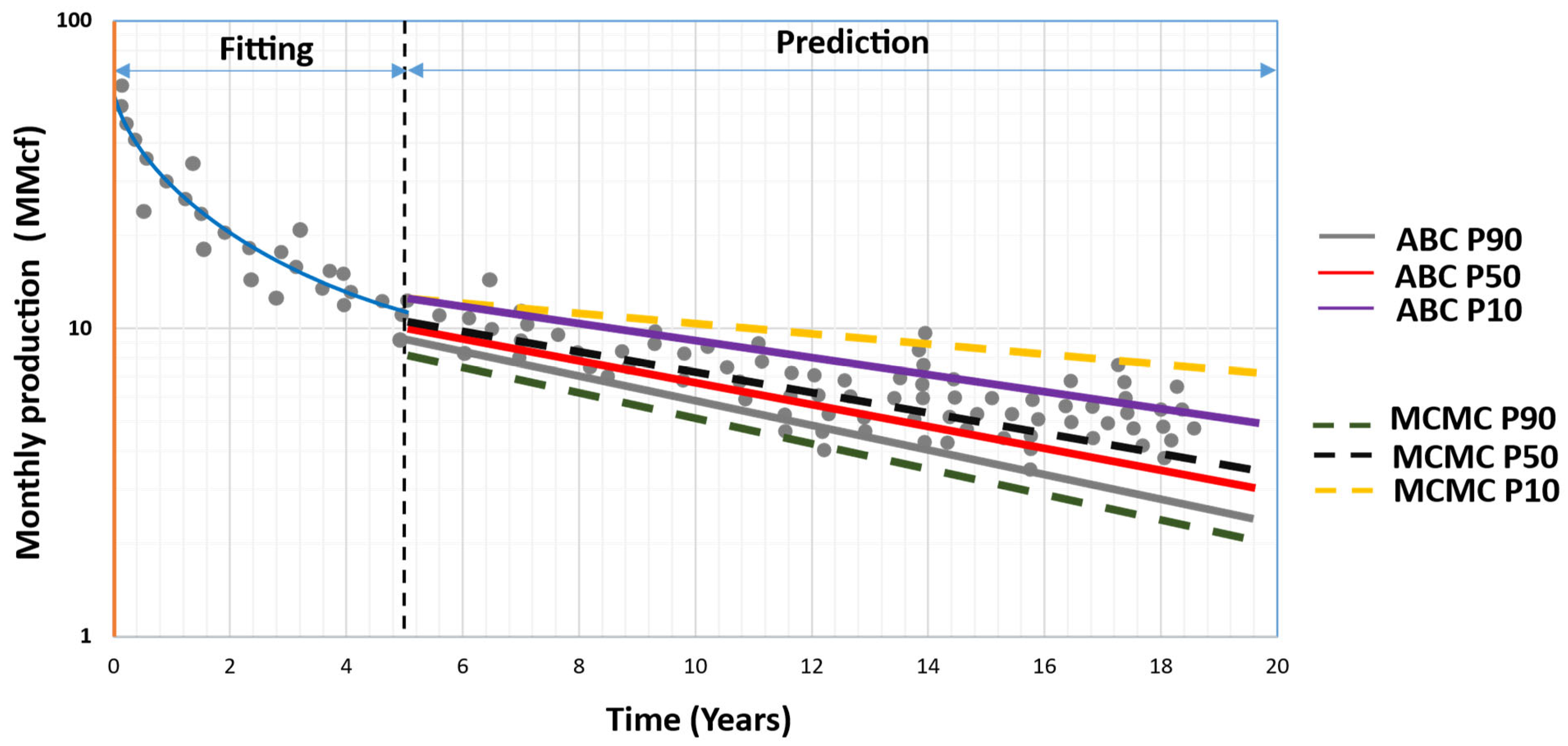
2.10. Paryani’s Approach (2017) [63]

Paryani et al. introduced their approach by combining the Arp and logistic growth (LGM) models in a probability study [63,64]. It was based on using the ABC sampling technique to approximate the complicated likelihood function of the model’s parameters by 1000 iterations. The approach was tested based on 121 oil and gas shale wells from two different fields. They denoted that their approach was much faster and could be combined with other deterministic DCA models. They indicated that LGM was much better than the Arps model and provided better CRs. They also compared their approach with Gong’s approach, as shown in Figure 7. Based on this comparison, although the two approaches bounded the production history from P₁₀ to P₉₀, Paryani’s approach had narrower intervals, which indicated low uncertainty.

2.11. Jimenez’s Approach (2017) [65]

Working on tight gas reservoirs, Jiménez introduced an approach to estimate the reserves based on a probability study [65]. In this work, they started with a parametric study on the Arps model’s parameters D_i and b to determine which parameter affected the reserve estimation more than the other. They denoted that the b parameter had a greater effect than the D_i parameter. This was known before this work as the b exponent is the controller of the curvature degree. Therefore, it affects the EUR value more than the D_i parameter does.

Applying different DCA models (hyperbolic Arps, SEPD, PLE, and LGM), the authors determined the EUR from each model. They proposed that SEPD was the conservative model among them. Therefore, they conducted a probability study to calculate P₁₀, P₅₀, and P₉₀ based on the MC simulation sampling technique and Chi-square distribution of the model parameters.

2.12. Joshi’s Approach (2018) [34]

Joshi used a time series analysis technique and a frequentist statistical analysis to quantify uncertainty [34]. The LGM and SEPD models were used to test their approach on 100 shale gas wells. Based on de-trending (i.e., subtracting the deterministic trend of the model from the actual data), the time series autoregressive integrated moving average (ARIMA) model was integrated with the LGM and SEPD models to generate the CIs (i.e., P₁₀, P₅₀, and P₉₀) around the production forecast.

It could be inferred that by increasing the available production data for fitting, the 80% CI became narrower (i.e., the uncertainty decreased), as shown in Figure 8.

Additionally, the authors also compared their approach with Gong’s approach, and they denoted that Gong’s approach was much more reliable as it had narrower CIs, as shown in Figure 9 [56]. The comparison could be considered as evidence of the effectiveness of the pDCA approach based on Bayesian analysis compared to the pDCA approach based on frequentist analysis.

2.13. Hong’s Approach (2019) [66]

Hong worked on nearly 69 unconventional oil wells from two different fields [66]. Four DCA models—Arps, SEPD, LGM, and Pan—were used. Using MATLAB software (MathWorks 2017a), they fitted each model 10 times using the cross-validation technique instead of the least squares estimation, which is commonly used in non-linear regression. This technique helped in improving the curve-fitting. The motivation behind this work was to determine which DCA model had the highest potential to perform pDCA among the other models. After choosing the prospective DCA model, the MC simulation sampling technique was used to generate a uniform distribution of the model’s parameters.

The authors concluded that the goodness of fitting was not a condition for the best model, but the best model was that one able to represent the actual flow behaviors. They also denoted that a large production history may not reduce the model’s uncertainty. Finally, and based on their work, Arps and LGM became more optimistic in estimating the reserve compared to the SEPD and Pan models. They did not indicate the number of iterations used to generate the uniform distribution or the computational time, which would have been important for evaluating their approach compared to other approaches.

2.14. Fanchi’s New Approach (2020) [67]

Fanchi introduced his pDCA approach after working on 15 shale oil wells in two different fields [67]. Using the MC simulation sampling technique, he created a uniform probability distribution of the used DCA models (Arps and SEPD) with 1000 iterations. The P₁₀, P₅₀, and P₉₀ were also estimated for both models. The study did not compare the results of the two proposed pDCA studies and denoted nothing about each study’s coverage. Therefore, it could not be considered a comparative analysis. The difference between this work and his previous work is that the domain of this study was shale oil while that of the previous work was shale gas.

2.15. Korde’s Approach (2021) [68]

Korde et al. worked on 74 conventional and unconventional wells (51 gas wells and 23 oil wells) to introduce their approach [68]. They used five DCA models (Arps, PLE, Duong, SEPD, and LGM). They assessed each DCA model based on three Bayesian sampling techniques (Gibbs, MH, and ABC). The probability distribution used was the maximum likelihood distribution. They introduced two ways to conduct the pDCA. The first was to choose one DCA model and evaluate the performance of the sampling techniques. They found that LGM performed well with all the sampling techniques except for MH. The second was to choose one sampling technique and evaluate the performance of all the DCA models. They found that the Gibbs algorithm performed well with all the DCA models except the Arps model. The computational time for each pDCA was between 2 and 25 s.

Figure 10 shows the different Bayesian sampling algorithms used in conjunction with the Arps model. It is easy to see how the interval width (IW) was the largest with the Gibbs algorithm and the lowest with the ABC algorithm. The author suggested that by preprocessing the data and reducing the noise, the IW was improved and the prediction errors were reduced.

The authors also concluded that, adding more production data to the pDCA model improved its results. Therefore, conducting more than pDCA helped to assure the results of the EUR.

The major differences between the aforementioned pDCA approaches are clearly stated and summarized in

Table 4. Summary of the pDCA approaches.

pDCA Model	Probabilistic Technique	Sampling Technique(s)	No. of Integrations	Computational Time	Used Probability Distribution
Jochen (1996)	Frequentist Analysis	MC Bootstrap	>100	6.5 h	-
Cheng (2010)	Frequentist Analysis	MC Bootstrap		More than 6.5 h	-
Minin (2011)	Bayesian Analysis	MC Latin Hypercube	-	-	Uniform
Brito (2012)	Bayesian Analysis	MC	-	-	Uniform
Gong (2011)	Bayesian Analysis	MCMC MH	2000	25 min	Approximate posterior
Gonzalez (2012)	Bayesian Analysis	MCMC MH	1000	25 min	Approximate posterior
Fanchi (2013)	Bayesian Analysis	MC	1000	-	Uniform
Kim (2014)	Bayesian Analysis	MC	5000	-	Triangle
Zhukovsky (2016)	Bayesian Analysis	MCMC MH	100,000	25 min	Approximate posterior
Paryani (2017)	Bayesian Analysis	MCMC ABC MC ABC Rejection ABC	10,000	Faster than Gong (2011)	Likelihood-free approximation
Jimenez (2017)	Bayesian Analysis	MC	-	-	Chi-square
Joshi (2018)	Frequentist Analysis	Time series
Hong (2019)	Bayesian Analysis	MC	-	-	Uniform
Fanchi (2020)	Bayesian Analysis	MC	1000	-	Uniform
Korde (2021)	Bayesian Analysis	MCMC Gibbs MH ABC	20,000	5–25 s	Likelihood
pDCA Model	The Study Domain			The Combined DCA Model(s)	Reference
Jochen (1996)	Conventional oil wells, two different fields			Arps	[54]
Cheng (2010)	Conventional mature oil and gas wells; 100 wells			Arps	[55]
Minin (2011)	Shale gas reservoirs; 150 gas wells			Arps	[57]
Brito (2012)	Conventional oil wells			PDE	[58]
Gong (2011)	Shale gas reservoirs; 197 gas wells			Arps	[56]
Gonzalez (2012)	Shale gas reservoirs; 197 gas wells			Arps, PLE, SEPD, and Duong	[5]
Fanchi (2013)	Shale gas reservoirs; 110 gas wells			Arps and SEPD	[60]
Kim (2014)	Shale gas reservoirs; 4 gas wells			Arps, SEPD, and PDE	[61]
Zhukovsky Approach (2016)	Shale reservoirs; 199 shale oil wells			EEDCA	[62]
Paryani (2017)	Unconventional reservoirs; 21 oil wells (Eagle Ford) and 100 gas wells (Barnett Shale)			Arps and LGM	[63,64]
Jimenez Approach (2017)	Tight gas reservoir; 1 gas well			Arps, SEPD, PLE, LGM, and Duong	[65]
Joshi Approach (2018)	Shale reservoirs; 100 shale gas wells			LGM and SEPD	[34]
Hong (2019)	Unconventional shale oil; Bakken field, 28 wells, and Midland field, 31 wells			Arps, SEPD, LGM, and Pan	[66]
Fanchi (2020)	Unconventional shale oil; Bakken field, 9 wells, and Eagle Ford, 6 wells			Arps and SEPD	[67]
Korde (2021)	Conventional and unconventional reservoirs; 23 oil wells and 51 gas wells			Arps, SEPD, PLE, Duong, and LGM	[68]

. The sampling techniques, the study domain, the selected models, and the used probability distributions are categorized and compared.

3. Conclusions and Recommendations

In this research, 15 different pDCA approaches were comprehensively reviewed and compared. The following conclusions can be drawn:

• The main differences among them are: (1) the selected DCA model(s) combined with the pDCA approach, (2) the used sampling technique and the assumed probability distributions of the model’s parameters, (3) the domain of the study, and (4) the computational time for each approach.
• The probability techniques of the approaches are mainly Bayesian analyses and only a few approaches are frequentist analyses. A frequentist analysis has a larger computational time than a Bayesian one. In addition, a Bayesian analysis is more effective, given narrower CIs than in a frequentist one.
• The bounds of the CIs and the CR change when using a different decline curve model(s) and when using different sampling algorithms. The ABC algorithm was the best at bounding the CIs when it was used with the Arps’s model. The assumption that the parameters that undergo sampling follow a certain probability distribution is important. The uniform distribution was the most common among the various approaches. Other assumptions such as posterior approximation and maximum likelihood are highly recommended.
• pDCA helps in quantifying the uncertainties related to DCA. Ranges of the EUR with a certain level of confidence are better than one deterministic EUR value that might be over- or under-estimated. The narrower the CIs, the more effective the pDCA approach. The computational time is critical, especially with approaches such as those of Cheng and Gong. The number of iterations in sampling is critical. As the number of iterations increases, the uncertainties decrease, but the computational time increases.
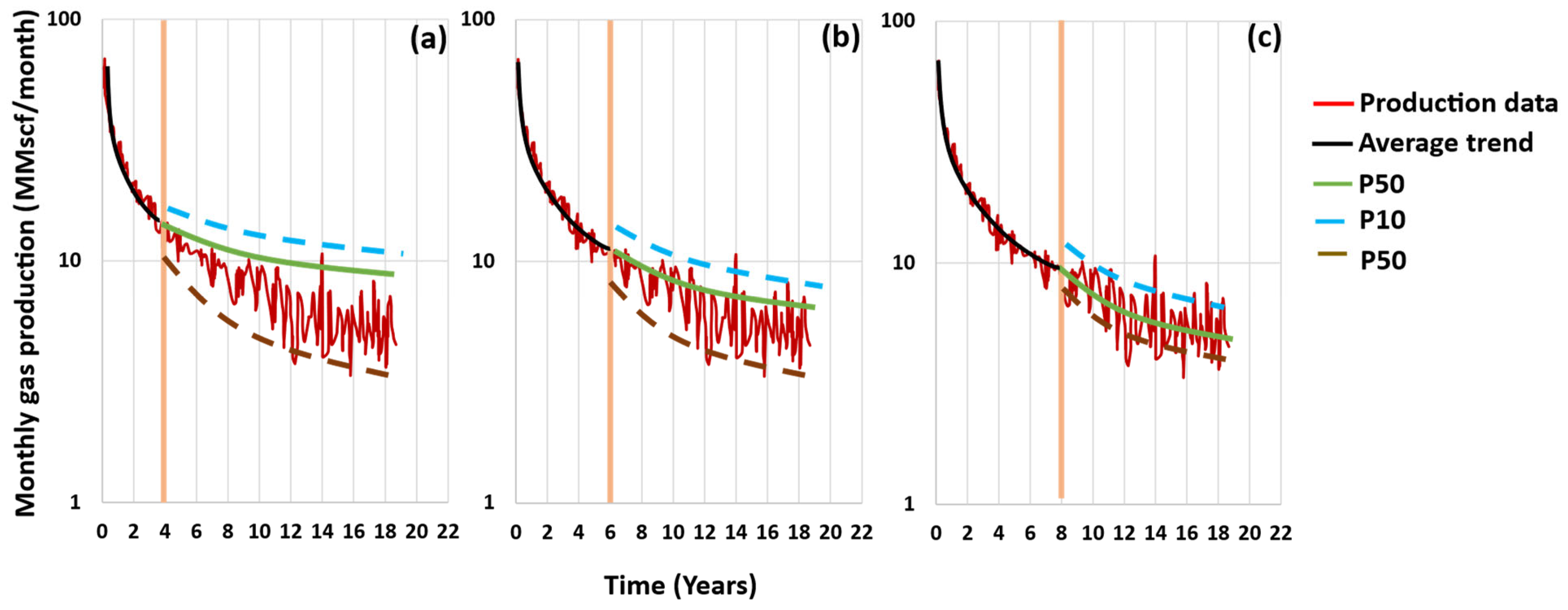
• As a recommendation, the larger the production history, the narrower the CI. In addition, improving data quality before an analysis by removing the outlier from the production data will reduce uncertainties and improve forecasting. Using more than one DCA model can also help in improving accuracy.

4. Suggestions for Future Research and Development

Based on this critical and detailed review of the previous works relevant to pDCA, it might be noticed that many research gaps should be filled and investigated. The following can be recommended for future research:

• Data size and data quality are crucial for any analysis. Therefore, testing the sensitivity of some of the proposed approaches to different data sizes and data qualities is recommended to gain deep insights into their performance under such conditions.
• Data of the early production period have a great impact on the whole analysis for two main reasons: (1) at an early time, especially in shale hydrocarbons, changes in flow regimes are severe, and (2) the flowback period is too noisy and could last for a long time. As result, further investigations of the impacts of this period of data on pDCA are recommended in order to develop more robust approaches.
• Computational time is critical for such analysis and is greatly affected by the number of iterations, the data size, and the used sampling algorithm. Based on this, more investigation is recommended about: (1) the sampling techniques and their effectiveness, (2) which critical parameters of a model should undergo probability distribution, and (3) which is the most effective and reliable distribution for each parameter.
• It is recommended to comprehensively use the new advancements in machine learning algorithms and supercomputing, which are capable of dealing with pDCA and include other production records such as pressure, water cut, chock size, periodic liquid loading, etc. in the analysis, which could lead to great improvements in production forecasting.

References

1. Liang, H.-B.; Zhang, L.-H.; Zhao, Y.-L.; Zhang, B.-N.; Chang, C.; Chen, M.; Bai, M.-X. Empirical Methods of Decline-Curve Analysis for Shale Gas Reservoirs: Review, Evaluation, and Application. J. Nat. Gas Sci. Eng. 2020, 83, 103531. [Google Scholar] [CrossRef]
2. Joshi, K.; Lee, J. Comparison of Various Deterministic Forecasting Techniques in Shale Gas Reservoirs. In Proceedings of the SPE Hydraulic Fracturing Technology Conference, The Woodlands, TX, USA, 4–6 February 2013; OnePetro: Richardson, TX, USA, 2013. [Google Scholar]
3. Chen, Q.; Wang, N.; Ruan, K.; Zhang, M. Selection of Production Decline Analysis Method of Shale Gas Well. Reserv. Eval. Dev. 2018, 8, 76–79. [Google Scholar]
4. Yuan, J.; Luo, D.; Feng, L. A Review of the Technical and Economic Evaluation Techniques for Shale Gas Development. Appl. Energy 2015, 148, 49–65. [Google Scholar] [CrossRef]
5. Gonzalez, R.; Gong, X.; McVay, D. Probabilistic decline curve analysis reliably quantifies uncertainty in shale gas reserves regardless of stage of depletion. In Proceedings of the SPE Eastern Regional Meeting, Lexington, KY, USA, 3–5 October 2012. [Google Scholar] [CrossRef]
6. Arps, J.J. Analysis of Decline Curves. Trans. AIME 1945, 160, 228–247. [Google Scholar] [CrossRef]
7. Ahmed, T. Analysis of Decline and Type Curves. In Reservoir Engineering Handbook; Elsevier: Amsterdam, The Netherlands, 2019; pp. 1227–1310. ISBN 978-0-12-813649-2. [Google Scholar]
8. Fetkovich, M.J. Decline-Curve Analysis Using Type Curves. SPE Form. Eval. 1980, 2, 637–656. [Google Scholar] [CrossRef]
9. Rongze, Y.; Wei, J.; Xiaowei, Z.; Wei, G.; Li, W.; Jingping, Z.; Meizhu, W. A Review of Empirical Production Decline Analysis Methods for Shale Gas Reservoir. China Pet. Explor. 2018, 23, 9. [Google Scholar]
10. Mahmoud, O.; Ibrahim, M.; Pieprzica, C.; Larsen, S. EUR Prediction for Unconventional Reservoirs: State of the Art and Field Case. In Proceedings of the SPE Trinidad and Tobago Section Energy Resources Conference, Port of Spain, Trinidad and Tobago, Virtual, 25 June 2018; OnePetro: Richardson, TX, USA, 2018. [Google Scholar]
11. Mostafa, S.; Hamid, K.; Tantawi, M. Studying Modern Decline Curve Analysis Models for Unconventional Reservoirs to Predict Performance of Shale Gas Reservoirs. JUSST 2021, 23, 36. [Google Scholar]
12. Yehia, T.; Khattab, H.; Tantawy, M.; Mahgoub, I. Improving the Shale Gas Production Data Using the Angular- Based Outlier Detector Machine Learning Algorithm. JUSST 2022, 24, 152–172. [Google Scholar]
13. Ibrahim, M.; Mahmoud, O.; Pieprzica, C. A New Look at Reserves Estimation of Unconventional Gas Reservoirs. In Proceedings of the SPE/AAPG/SEG Unconventional Resources Technology Conference, Houston, TX, USA, 23 July 2018; OnePetro: Richardson, TX, USA, 2018. [Google Scholar]
14. Zhang, R.; Zhang, L.; Tang, H.; Chen, S.; Zhao, Y.; Wu, J.; Wang, K. A Simulator for Production Prediction of Multistage Fractured Horizontal Well in Shale Gas Reservoir Considering Complex Fracture Geometry. J. Nat. Gas Sci. Eng. 2019, 67, 14–29. [Google Scholar] [CrossRef]
15. You, X.-T.; Liu, J.-Y.; Jia, C.-S.; Li, J.; Liao, X.-Y.; Zheng, A.-W. Production Data Analysis of Shale Gas Using Fractal Model and Fuzzy Theory: Evaluating Fracturing Heterogeneity. Appl. Energy 2019, 250, 1246–1259. [Google Scholar] [CrossRef]
16. Nwaobi, U.; Anandarajah, G. A Critical Review of Shale Gas Production Analysis and Forecast Methods. Saudi J. Eng. Technol. (SJEAT) 2018, 5, 276–285. [Google Scholar]
17. Brantson, E.T.; Ju, B.; Ziggah, Y.Y.; Akwensi, P.H.; Sun, Y.; Wu, D.; Addo, B.J. Forecasting of Horizontal Gas Well Production Decline in Unconventional Reservoirs Using Productivity, Soft Computing and Swarm Intelligence Models. Nat. Resour. Res. 2019, 28, 717–756. [Google Scholar] [CrossRef]
18. Wahba, A.; Khattab, H.; Gawish, A. A Study of Modern Decline Curve Analysis Models Based on Flow Regime Identification. JUSST 2022, 24, 26. [Google Scholar]
19. Wahba, A.M.; Khattab, H.M.; Tantawy, M.A.; Gawish, A.A. Modern Decline Curve Analysis of Unconventional Reservoirs: A Comparative Study Using Actual Data. J. Pet. Min. Eng. 2022, 24, 51–65. [Google Scholar] [CrossRef]
20. Yehia, T.; Khattab, H.; Tantawy, M.; Mahgoub, I. Removing the Outlier from the Production Data for the Decline Curve Analysis of Shale Gas Reservoirs: A Comparative Study Using Machine Learning. ACS Omega 2022, 7, 32046–32061. [Google Scholar] [CrossRef]
21. Ahmed, T. Modern Decline Curve Analysis. In Reservoir Engineering Handbook; Elsevier: Amsterdam, The Netherlands, 2019; pp. 1389–1461. ISBN 978-0-12-813649-2. [Google Scholar]
22. Cheng, Y. Improving Reserves Estimates From Decline-Curve Analysis of Tight and Multilayer Gas Wells. SPE Reserv. Eval. Eng. 2008, 11, 912–920. [Google Scholar] [CrossRef]
23. Ilk, D.; Rushing, J.A.; Perego, A.D.; Blasingame, T.A. Exponential vs. Hyperbolic Decline in Tight Gas Sands: Understanding the Origin and Implications for Reserve Estimates Using Arps’ Decline Curves. In Proceedings of the SPE Annual Technical Conference and Exhibition, Denver, CO, USA, 21 September 2008; p. SPE-116731-MS. [Google Scholar]
24. Ilk, D.; Perego, A.D.; Rushing, J.A.; Blasingame, T.A. Integrating Multiple Production Analysis Techniques To Assess Tight Gas Sand Reserves: Defining a New Paradigm for Industry Best Practices. In Proceedings of the CIPC/SPE Gas Technology Symposium 2008 Joint Conference, Calgary, AB, Canada, 16 June 2008; p. SPE-114947-MS. [Google Scholar]
25. Valko, P.P. Assigning Value to Stimulation in the Barnett Shale: A Simultaneous Analysis of 7000 plus Production Hystories and Well Completion Records. In Proceedings of the SPE hydraulic fracturing technology conference, The Woodlands, TX, USA, 19 January 2009; OnePetro: Richardson, TX, USA, 2009. [Google Scholar]
26. Valkó, P.P.; Lee, W.J. A Better Way to Forecast Production from Unconventional Gas Wells. In Proceedings of the SPE Annual Technical Conference and Exhibition, Florence, Italy, 19 September 2010; p. SPE-134231-MS. [Google Scholar]
27. Duong, A.N. An Unconventional Rate Decline Approach for Tight and Fracture-Dominated Gas Wells. In Proceedings of the Canadian Unconventional Resources and International Petroleum Conference, Calgary, AB, Canada, 19 October 2010; p. SPE-137748-MS. [Google Scholar]
28. Duong, A.N. Rate-Decline Analysis for Fracture-Dominated Shale Reservoirs. SPE Reserv. Eval. Eng. 2011, 14, 377–387. [Google Scholar] [CrossRef]
29. Clark, A.J.; Lake, L.W.; Patzek, T.W. Production Forecasting with Logistic Growth Models. In Proceedings of the SPE Annual Technical Conference and Exhibition, Denver, CO, USA, 30 October 2011; p. SPE-144790-MS. [Google Scholar]
30. Zhang, H.; Cocco, M.; Rietz, D.; Cagle, A.; Lee, J. An Empirical Extended Exponential Decline Curve for Shale Reservoirs. In Proceedings of the SPE Annual Technical Conference and Exhibition, Houston, TX, USA, 28 September 2015; p. D031S031R007. [Google Scholar]
31. Wattenbarger, R.A.; El-Banbi, A.H.; Villegas, M.E.; Maggard, J.B. Production Analysis of Linear Flow Into Fractured Tight Gas Wells. In Proceedings of the SPE Rocky Mountain Regional/Low-Permeability Reservoirs Symposium, Denver, CO, USA, 5 April 1998; OnePetro: Richardson, TX, USA, 1998. [Google Scholar] [CrossRef]
32. Mahmoud, O.; Elnekhaily, S.; Hegazy, G. Estimating Ultimate Recoveries of Unconventional Reservoirs: Knowledge Gained from the Developments Worldwide and Egyptian Challenges. Int. J. Ind. Sustain. Dev. 2020, 1, 60–70. [Google Scholar] [CrossRef]
33. Yehia, T.; Wahba, A.; Mostafa, S.; Mahmoud, O. Suitability of Different Machine Learning Outlier Detection Algorithms to Improve Shale Gas Production Data for Effective Decline Curve Analysis. Energies 2022, 15, 8835. [Google Scholar] [CrossRef]
34. Joshi, K.G.; Awoleke, O.O.; Mohabbat, A. Uncertainty Quantification of Gas Production in the Barnett Shale Using Time Series Analysis. In Proceedings of the SPE Western Regional Meeting, Garden Grove, CA, USA, 22 April 2018; OnePetro: Richardson, TX, USA, 2018. [Google Scholar]
35. Yehia, T.; Abdelhafiz, M.M.; Hegazy, G.M.; Elnekhaily, S.A.; Mahmoud, O. A Comprehensive Review of Deterministic Decline Curve Analysis for Oil and Gas Reservoirs. Geoenergy Sci. Eng. 2023, 226, 211775. [Google Scholar] [CrossRef]
36. Manda, P.; Nkazi, D.B. The Evaluation and Sensitivity of Decline Curve Modelling. Energies 2020, 13, 2765. [Google Scholar] [CrossRef]
37. Martyushev, D.A.; Ponomareva, I.N.; Galkin, V.I. Conditions for Effective Application of the Decline Curve Analysis Method. Energies 2021, 14, 6461. [Google Scholar] [CrossRef]
38. Maraggi, L.M.R.; Lake, L.W.; Lake, L.W.; Walsh, M.P. Bayesian Predictive Performance Assessment of Rate-Time Models for Unconventional Production Forecasting. In Proceedings of the 82nd EAGE Annual Conference & Exhibition, Amsterdam, The Netherlands, 18–21 October 2021. [Google Scholar] [CrossRef]
39. Capen, E.C. Probabilistic Reserves! Here at Last? SPE Reserv. Eval. Eng. 2001, 4, 387–394. [Google Scholar] [CrossRef]
40. Egbe, U.C.; Awoleke, O.O.; Olorode, O.; Goddard, S.D. On the Application of Probabilistic Decline Curve Analysis to Unconventional Reservoirs. SPE Reserv. Eval. Eng. 2022, 26, 1–17. [Google Scholar] [CrossRef]
41. Asante, J.; Ampomah, W.; Rose-Coss, D.; Cather, M.; Balch, R. Probabilistic Assessment and Uncertainty Analysis of CO2 Storage Capacity of the Morrow B Sandstone—Farnsworth Field Unit. Energies 2021, 14, 7765. [Google Scholar] [CrossRef]
42. Gelman, A.; Vehtari, A.; Simpson, D.; Margossian, C.C.; Carpenter, B.; Yao, Y.; Kennedy, L.; Gabry, J.; Bürkner, P.-C.; Modrák, M. Bayesian Workflow. arXiv 2020, arXiv:2011.01808. [Google Scholar] [CrossRef]
43. Baluev, R.V. Comparing the Frequentist and Bayesian Periodic Signal Detection: Rates\n of Statistical Mistakes and Sensitivity to Priors. Mon. Not. R. Astron. Soc. 2022, 512, 5520–5534. [Google Scholar] [CrossRef]
44. Yuhun, P.; Awoleke, O.O.; Goddard, S.D. Using Rate Transient Analysis and Bayesian Algorithms for Reservoir Characterization in Unconventional Gas Wells during Linear Flow. SPE Reserv. Eval. Eng. 2021, 24, 733–751. [Google Scholar] [CrossRef]
45. Lambert, B. A Student’s Guide to Bayesian Statistics; Sage: Newcastle, UK, 2018; pp. 1–520. [Google Scholar]
46. Maior, C.B.S.; Macedo, J.B.; Lins, I.D.; Moura, M.C.; Azevedo, R.V.; De Santana, J.M.M.; da Silva, M.J.; da Silva, M.F.; Magalhães, M.V.C. Bayesian Prior Distribution Based on Generic Data and Experts’ Opinion: A Case Study in the O&G Industry. J. Pet. Sci. Eng. 2021, 210, 109891. [Google Scholar] [CrossRef]
47. Maraggi, L.M.R.; Lake, L.W.; Walsh, M.P. Using Bayesian Leave-One-Out and Leave-Future-Out Cross-Validation to Evaluate the Performance of Rate-Time Models to Forecast Production of Tight-Oil Wells. SPE Reserv. Eval. Eng. 2022, 25, 730–750. [Google Scholar] [CrossRef]
48. Cummings, M.P.; Handley, S.A.; Myers, D.S.; Reed, D.L.; Rokas, A.; Winka, K. Comparing Bootstrap and Posterior Probability Values in the Four-Taxon Case. Syst. Biol. 2003, 52, 477–487. [Google Scholar] [CrossRef] [PubMed]
49. Qian, S.S.; Stow, C.A.; Borsuk, M.E. On Monte Carlo Methods for Bayesian Inference. Ecol. Model. 2003, 159, 269–277. [Google Scholar] [CrossRef]
50. Tillé, Y. Sampling Algorithms; Springer Series in Statistics; Springer: New York, NY, USA, 2006; ISBN 978-0-387-30814-2. [Google Scholar]
51. Makarova, A.A.; Mantorova, I.V.; Kovalev, D.A.; Kutovoy, I.N. The Modeling of Mineral Water Fields Data Structure. In Proceedings of the 2021 IEEE Conference of Russian Young Researchers in Electrical and Electronic Engineering (ElConRus), St. Petersburg, Russia, 26–29 January 2021; pp. 517–521. [Google Scholar]
52. Makarova, A.A.; Kaliberda, I.V.; Kovalev, D.A.; Pershin, I.M. Modeling a Production Well Flow Control System Using the Example of the Verkhneberezovskaya Area. In Proceedings of the 2022 Conference of Russian Young Researchers in Electrical and Electronic Engineering (ElConRus), Saint Petersburg, Russia, 25–28 January 2022; pp. 760–764. [Google Scholar]
53. Martirosyan, A.V.; Ilyushin, Y.V. Modeling of the Natural Objects’ Temperature Field Distribution Using a Supercomputer. Informatics 2022, 9, 62. [Google Scholar] [CrossRef]
54. Jochen, V.A.; Spivey, J.P. Probabilistic Reserves Estimation Using Decline Curve Analysis with the Bootstrap Method. In Proceedings of the SPE Annual Technical Conference and Exhibition, Denver, CO, USA, 6 October 1996; OnePetro: Richardson, TX, USA, 1996. [Google Scholar]
55. Cheng, Y.; Wang, Y.; McVay, D.A.A.; Lee, W.J.J. Practical Application of a Probabilistic Approach to Estimate Reserves Using Production Decline Data. SPE Econ. Manag. 2010, 2, 19–31. [Google Scholar] [CrossRef]
56. Gong, X.; Gonzalez, R.; McVay, D.A.; Hart, J.D. Bayesian Probabilistic Decline-Curve Analysis Reliably Quantifies Uncertainty in Shale-Well-Production Forecasts. SPE J. 2014, 19, 1047–1057. [Google Scholar] [CrossRef]
57. Minin, A.; Guerra, L.; Colombo, I. Unconventional Reservoirs Probabilistic Reserve Estimation Using Decline Curves. In Proceedings of the International Petroleum Technology Conference, Bangkok, Thailand, 15 November 2011; p. IPTC-14801-MS. [Google Scholar]
58. Brito, L.E.; Paz, F.; Belisario, D. Probabilistic Production Forecasts Using Decline Envelopes. In Proceedings of the SPE Latin America and Caribbean Petroleum Engineering Conference, Mexico City, Mexico, 16 April 2012; p. SPE-152392-MS. [Google Scholar]
59. Gong, X.; Gonzalez, R.; McVay, D.; Hart, J. Bayesian Probabilistic Decline Curve Analysis Quantifies Shale Gas Reserves Uncertainty. In Proceedings of the Canadian Unconventional Resources Conference, Calgary, AB, Canada, 15 November 2011; p. SPE-147588-MS. [Google Scholar]
60. Fanchi, J.R.; Cooksey, M.J.; Lehman, K.M.; Smith, A.; Fanchi, A.C.; Fanchi, C.J. Probabilistic Decline Curve Analysis of Barnett, Fayetteville, Haynesville, and Woodford Gas Shales. J. Pet. Sci. Eng. 2013, 109, 308–311. [Google Scholar] [CrossRef]
61. Kim, J.-S.; Shin, H.-J.; Lim, J.-S. Application of a Probabilistic Method to the Forecast of Production Rate Using a Decline Curve Analysis of Shale Gas Play. In Proceedings of the Twenty-Fourth International Ocean and Polar Engineering Conference, Busan, Republic of Korea, 15–20 June 2014; p. ISOPE-I-14-158. [Google Scholar]
62. Zhukovsky, I.D.; Mendoza, R.C.; King, M.J.; Lee, W.J. Uncertainty Quantification in the EUR of Eagle Ford Shale Wells Using Probabilistic Decline-Curve Analysis with a Novel Model. In Proceedings of the Abu Dhabi International Petroleum Exhibition & Conference, Abu Dhabi, United Arab Emirates, 7 November 2016; p. D021S049R005. [Google Scholar]
63. Paryani, M. Approximate Bayesian Computation for Probabilistic Decline Curve Analysis in Unconventional Reservoirs. Master’s Thesis, University of Alaska Fairbanks, College, AK, USA, 2015. Available online: https://hdl.handle.net/11122/6383 (accessed on 15 December 2022).
64. Paryani, M.; Awoleke, O.O.; Ahmadi, M.; Hanks, C.; Barry, R. Approximate Bayesian Computation for Probabilistic Decline-Curve Analysis in Unconventional Reservoirs. SPE Reserv. Eval. Eng. 2017, 20, 478–485. [Google Scholar] [CrossRef]
65. Jiménez, E.T.; Cervantes, R.J.; Magnelli, D.E.; Dabrowski, A. Probabilistic Approach of Advanced Decline Curve Analysis for Tight Gas Reserves Estimation Obtained from Public Data Base. In Proceedings of the SPE Latin America and Caribbean Petroleum Engineering Conference, Buenos Aires, Argentina, 17 May 2017; p. D021S009R006. [Google Scholar]
66. Hong, A.; Bratvold, R.B.; Lake, L.W.; Ruiz Maraggi, L.M. Integrating Model Uncertainty in Probabilistic Decline-Curve Analysis for Unconventional-Oil-Production Forecasting. SPE Reserv. Eval. Eng. 2019, 22, 861–876. [Google Scholar] [CrossRef]
67. Fanchi, J. Decline Curve Analysis of Shale Oil Production Using a Constrained Monte Carlo Technique. J. Basic Appl. Sci. 2020, 16, 61–67. [Google Scholar] [CrossRef]
68. Korde, A.; Goddard, S.D.; Awoleke, O.O. Probabilistic Decline Curve Analysis in the Permian Basin Using Bayesian and Approximate Bayesian Inference. SPE Reserv. Eval. Eng. 2021, 24, 536–551. [Google Scholar] [CrossRef]
Figure 1. Differences when using the ordinary least squares (OLS) versus weighted least squares (WLS) regression techniques with the same DCA model (Reproduced from [34]).
Energies 16 04117 g001
Figure 2. A scheme that shows the modifications to Jochen’s approach by Cheng.
Energies 16 04117 g002
Figure 3. The “backward scenario”.
Energies 16 04117 g003
Figure 4. A comparison between Gong’s approach and the MBM approach.
Energies 16 04117 g004
Figure 5. Summary of Brito’s approach.
Energies 16 04117 g005
Figure 6. Summary of Franchi’s approach.
Energies 16 04117 g006
Figure 7. A comparison between Paryani’s and Gong’s approaches.
Energies 16 04117 g007
Figure 8. Results of Joshi’s approach when increasing the production data being fitted from (ac).
Energies 16 04117 g008
Figure 9. A comparison between Gong’s and Joshi’s approaches.
Energies 16 04117 g009
Figure 10. The different Bayesian sampling algorithms that were used in conjunction with the Arps model: (a) MH algorithm, (b) Gibbs algorithm, and (c) ABC algorithm.
Energies 16 04117 g010