Why Does the PV Solar Power Plant Operate Ineffectively?

Abstract

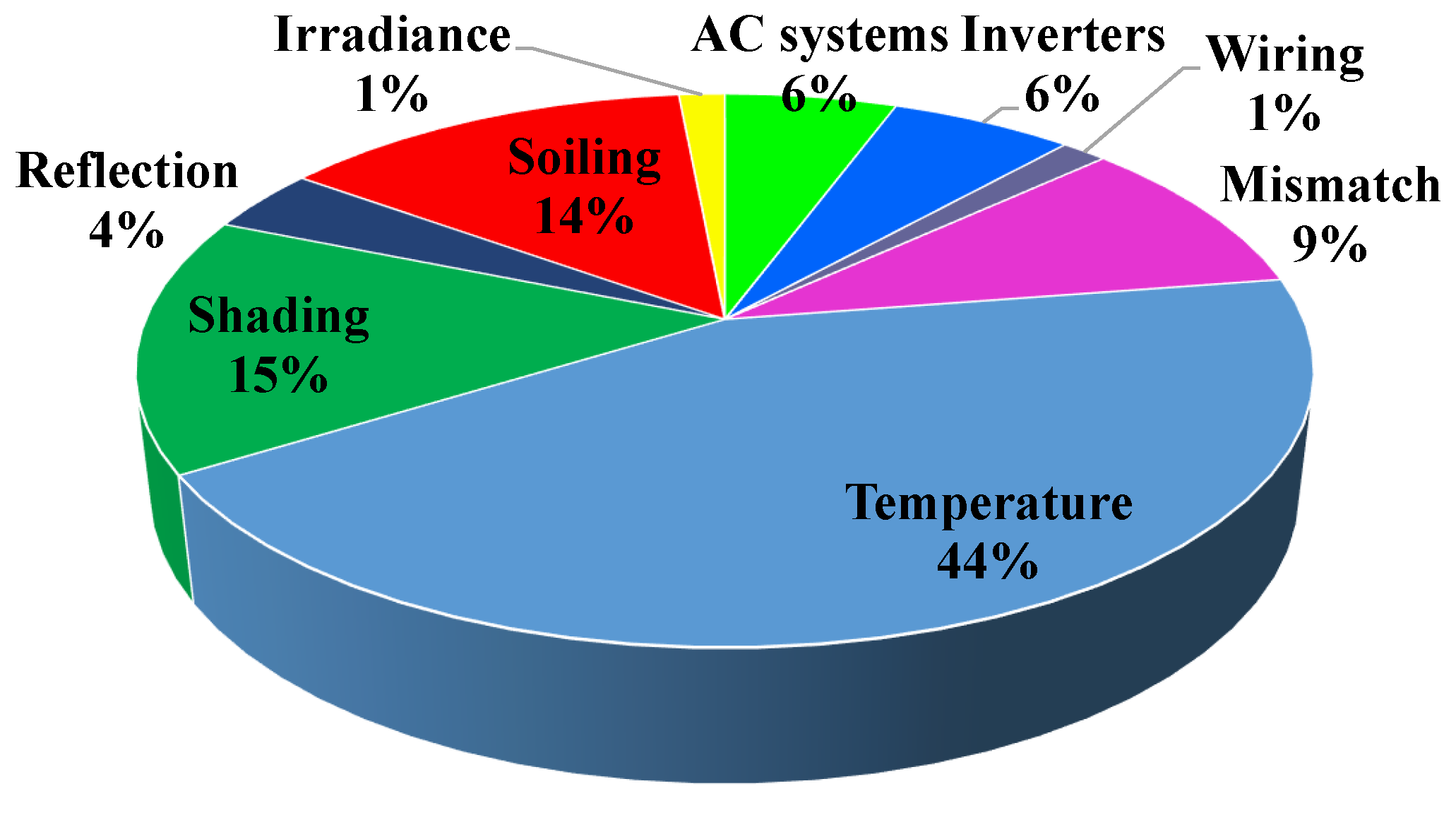
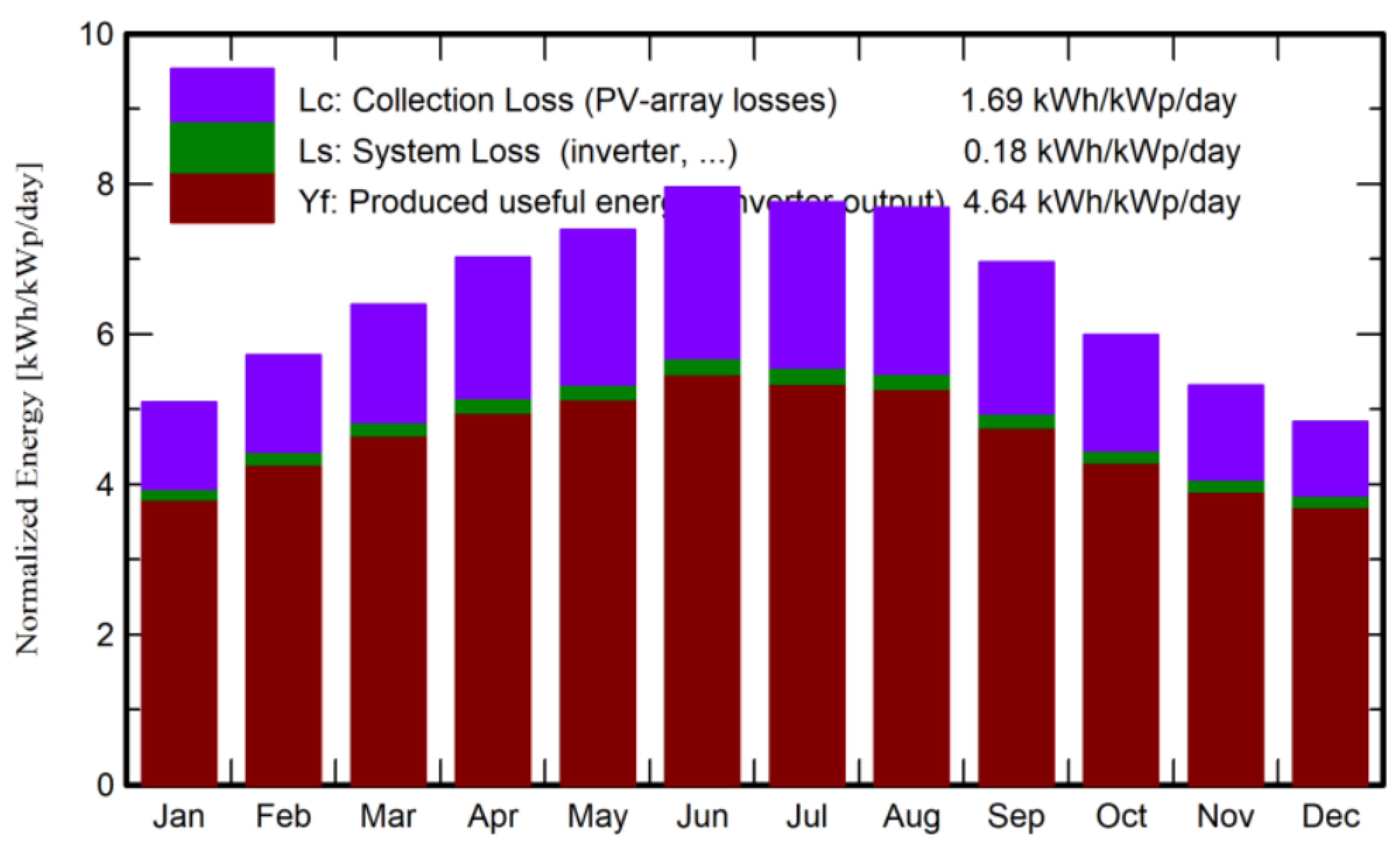
Quality, reliability, and durability are the key features of photovoltaic (PV) solar system design, production, and operation. They are considered when manufacturing every cell and designing the entire system. Achieving these key features ensures that the PV solar system performs satisfactorily and offers years of trouble-free operation, even in adverse conditions. In each cell, the quality of the raw material should meet the quality standards. The fulfillment of the quality management system requires every part that goes into the PV solar system to undergo extensive testing in laboratories and environments to ensure it meets expectations. Hence, every MWh of electricity generated by the PV solar system is counted, the losses should be examined, and the PV system’s returns should be maximized. There are many types of losses in the PV solar system; these losses are identified and quantified based on knowledge and experience. They can be classified into two major blocks: optical and electrical losses. The optical losses include, but are not limited to, partial shading losses, far shading losses, near shading losses, incident angle modifier (IAM) losses, soiling losses, potential induced degradation (PID) losses, temperature losses, light-induced degradation (LID) losses, PV yearly degradation losses, array mismatch losses, and module quality losses. In addition, there are cable losses inside the PV solar power system, inverter losses, transformer losses, and transmission line losses. Thus, this work reviews the losses in the PV solar system in general and the 103 MWp grid-tied Al Quweira PV power plant/Aqaba, mainly using PVsyst software. The annual performance ratio (PR) is $79.5\%$, and the efficiency $\left(\eta \right)$ under standard test conditions (STC) is $16.49\%$. The normalized production is 4.64 kWh/kWp/day, the array loss is 1.69 kWh/kWp/day, and the system loss is 0.18 kWh/kWp/day. Understanding factors that impact the PV system production losses is the key to obtaining an accurate production estimation. It enhances the annual energy and yield generated from the power plant. This review benefits investors, energy professionals, manufacturers, installers, and project developers by allowing them to maximize energy generation from PV solar systems and increase the number of solar irradiation incidents on PV modules.

1. Introduction

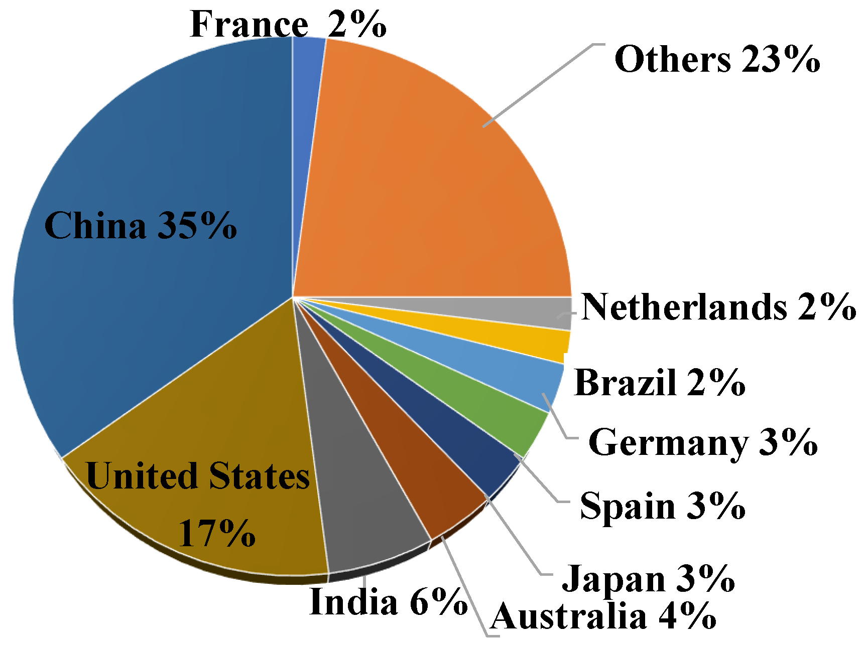
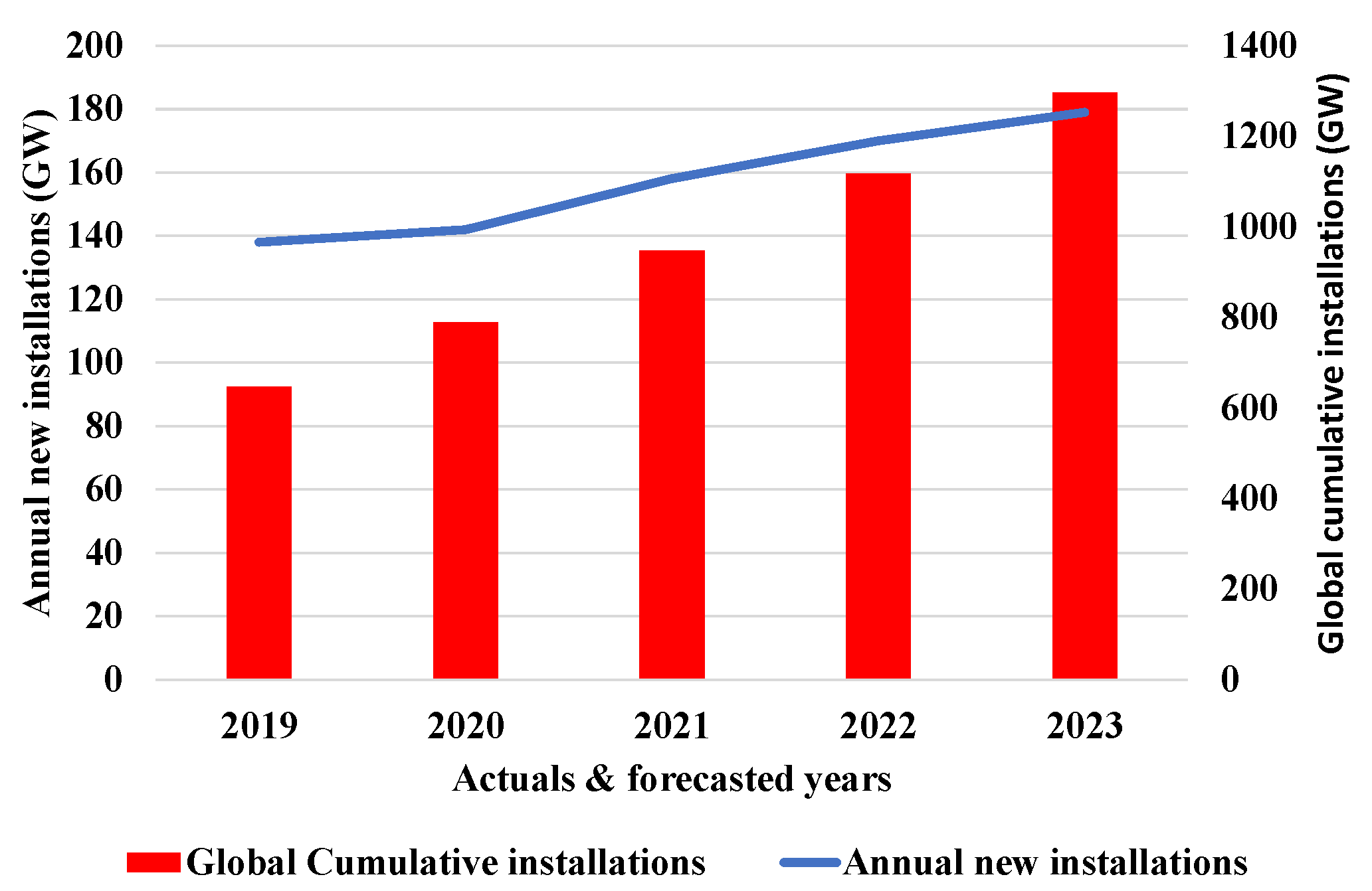
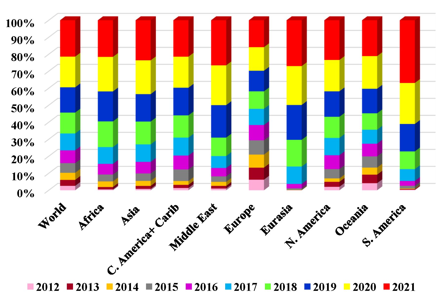
Electrical companies strive to exploit renewable energy’s vast potential to meet the growing energy requirements. The high penetration of photovoltaic (PV) power plants in electrical generation is evident due to the global increase in their installation capacity year-by-year, as shown in Figure 1 and Figure 2, respectively. Plummeting prices and the rising efficiency of the plant enhance the installed capacity. At the end of 2021, the total installed capacity was around 947 GW, as shown in Figure 3.

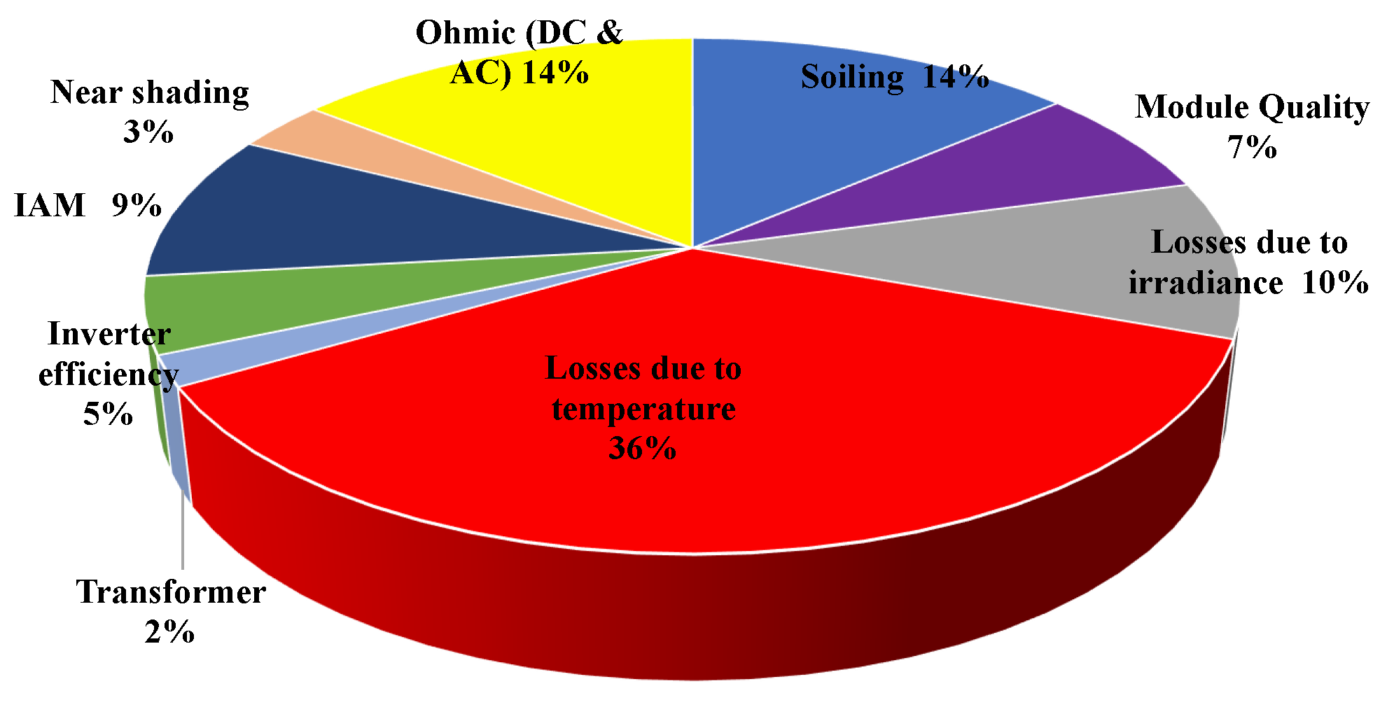
New technologies tend to come with unknown risks; investors must know these. Every technology brings a new mode of failure and a unique design. The solar system’s efficiency should be calculated under standard test conditions (STC). The STC are the industry standards for conditions under which solar panels are tested using a fixed set of conditions. Thus, the solar panels can be more accurately compared and rated against each other. The STC are specified as a temperature of $25{}^{\circ }$C for the cell itself, not the surrounding ambient temperature, and an irradiance of 1000 W/m². This refers to the amount of energy falling on a given area at a given time. Additionally, the air mass (AM) under the STC is 1.5. This refers to the amount of light that has to pass through the Earth’s atmosphere before it can hit the Earth’s surface [1]. Thus, a solar panel efficiency of $20\%$ with a 1 m² surface area would produce 200 W of energy. The energy production of the PV power plant depends on many factors, ranging from the array of characteristics, environmental factors, and how the plant is designed and installed. Plant losses are considered for calculating efficiency and establishing ways to enhance performance. Literature reviews have discussed PV power plant failures [2,3] and some types of losses. This review sheds light on the losses in the cell and system. These losses provide an important framework for the solar cell fabrication process, system design, and layout. They can be classified mainly into optical and electrical losses and combinations. These losses can also be classified based on DC and AC side losses. Classification of these losses can compare the different solar plant arrays in technology fabrication and manufacturing. These losses are included in Figure 4 and Figure 5, respectively. Soiling losses [4,5], shading losses [6], incidence angle modifier (IAM) losses [7], potential induced degradation (PID) [8,9], LID loss [10], temperature losses [11], PV yearly degradation [12], array mismatch losses [13,14], module quality losses [15], and electrical losses are presented. Electrical losses include AC losses, inverter losses [16,17], and transformer losses [18,19]. Typically, solar cells display an efficiency of about $20\%$ [20]. This means that they could convert $20\%$ of the incoming energy from sunlight into electric current. However, for light-induced degradation (LID) losses only, within the hours of operation, the efficiency drops to $18\%$, which represents a $2\%$ drop in total electric generation [21]. Losing $2\%$ of 790 GW is a significant problem. Thus, there is significant potential for electricity to be lost. It is no wonder that researchers are hunting down the cause of this problem. Many researchers have investigated PV losses through surveys [22,23]. This work provides the necessary information for project developers, energy professionals, investors, policymakers, and users regarding the actual losses situation of the PV solar planet.

Figure 1. PV power plant installation forecast for 2021 (GW) [24].

Figure 1. PV power plant installation forecast for 2021 (GW) [24].

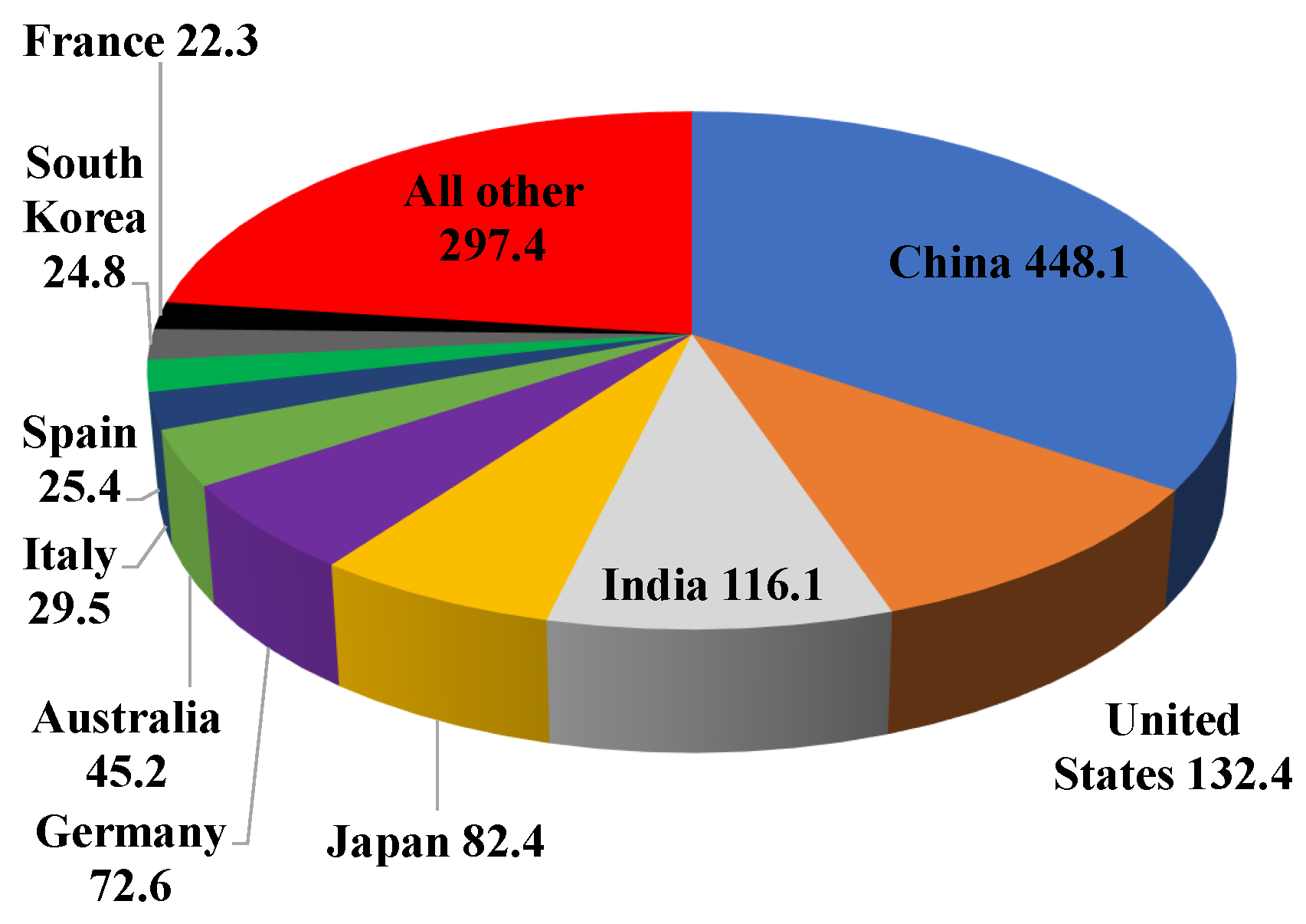
Figure 2. Top 10 countries with a total cumulative PV power plant installation capacity of 1296 GW in 2023 [25].

Figure 2. Top 10 countries with a total cumulative PV power plant installation capacity of 1296 GW in 2023 [25].

Figure 3. World market for the total cumulative PV power plant & annual net new installations (GW) [25].

Figure 3. World market for the total cumulative PV power plant & annual net new installations (GW) [25].

Figure 4. An example of losses in a PV power plant [26].

Figure 4. An example of losses in a PV power plant [26].

Figure 5. An example of losses in a PV power plant [27].

Figure 5. An example of losses in a PV power plant [27].

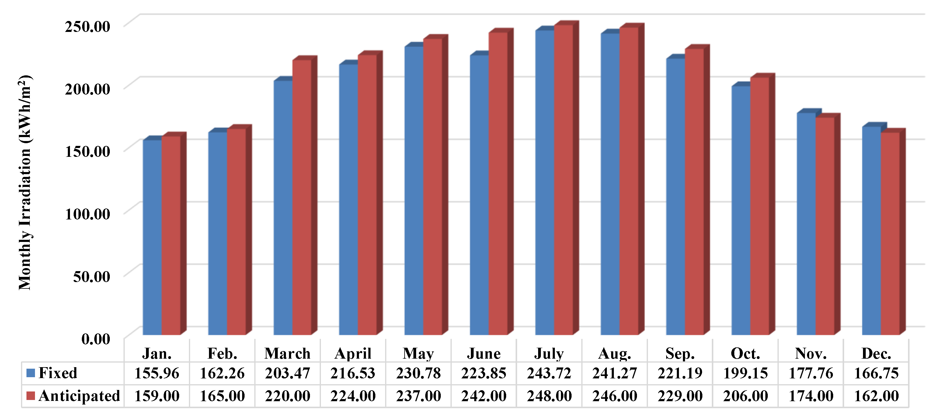
PV solar power plants have had the most significant generation growth among renewable energy resources globally. They exceeded 1000 terawatt-hours (TWh) by the end of 2021. Records show that the increment was 179 TWh that year, as shown in Figure 6. This has become the lowest-cost option for new electricity generation installations for most of the world. The average annual growth was $25\%$ in 2022–2030 [28]. A strategic policy and tremendous effort from the public and private sectors must be established to achieve a net zero emissions scenario by 2050. PV solar power plants account for $3.6\%$ of global electricity generation and remain the third-largest renewable electricity technology after wind energy and hydropower generation. In 2021, China was responsible for about $38\%$ of the generation growth as it installed a large PV solar power plant capacity. The USA had the second-largest generation growth, about $17\%$, and the European Union had the third-largest $10\%$. As a result of this strong growth, experts have amended their outlook for 2022, anticipating new systems to total between 204 and 252 [28].

This paper is organized as follows. Section 2 presents the current status of renewable energy in Jordan. In Section 3, PV power plant optical losses are explained. Next, PV power plant electrical losses are investigated in Section 4, followed by optimization of the PV solar power plant design in Section 5. A real case study is analyzed in Section 6. The results and discussion are presented in Section 7. Finally, the conclusions are mentioned in Section 8.

2. Current Status of Renewable Energy in Jordan

Jordan is one of the world’s most energy-insecure countries, importing $96\%$ of its energy needs. The energy challenge in Jordan is more critical today than ever; this is why the government of Jordan has issued an energy efficiency and renewable energy law which provides incentives for sustainable energy solutions. The government ambitiously aims to slash its fossil fuel bill by making green energy $20\%$ of its overall power consumption by 2024. Jordan has become aware of the importance of solar power for reducing energy costs. Jordan is blessed with over 300 days of sunshine yearly and is considered one of the sunbelt countries. Unsurprisingly, solar energy projects have quickly become the government’s hot choice. A legal framework has been developed in Jordan to attract investors and the government’s commitment to renewable energy. Thus, the Kingdom has officially made its place on the renewable energy map. In 2012, Jordan encouraged the installation of solar cells in houses, enabling consumers to store or buy the solar energy surplus. In 2018, investments in solar energy amounted to 30 fully implemented and under-construction projects. The actual investment amounted to $\$1.938$ [29] billion. Most solar energy projects are located in the south, where there is higher solar radiation, making this sector a promising investment opportunity. Thus, it is expected that there will be an increase in the reliance on solar energy in Jordan in the coming years. Therefore, as a case study, this review investigates the state-of-the-art research on losses in PV power plants in general and in Jordan’s Quweira PV power plant in particular. Jordan’s Ministry of Energy and Minerals Resources (MEMR) is the project owner of the Quweira PV power plant, and Tsk-Enviromena JV is the project contractor. At the Jordanian transmission network at the National Electric Power Company (NEPCO), the Al-Quweira PV solar system is integrated at the 132/33 kV substation via two step-up transformers.

Table 1. Power generation stations are connected on transmission lines (MW) based on fuel use in Jordan [29].

Year	Steam	Gas		Combined Cycle	Diesel Units	Renewable Energy				Total
		Diesel	Natural Gas			Hydrolic	Wind	PV Solar		Renewable	Nonrenewable
2016	605	-	307	2044	814	6	198	194		398	3770
2017	605	-	228	2044	814	6	198	204		408	3691
2018	605	-	83	2740	814	6	198	449		735	4242
2019	605	-	83	2740	814	6	198	637		1012	4242
2020	363	-	83	2740	814	6	198	900		1424	4000

shows generated power stations connected to transmission lines (MW) based on the fuel used.

Table 2. Renewable energy projects connected to the transmission system in 2020 in Jordan [29].

Project	Generation Capacity (MW)
Mass Group Holding Ltd/Tafila	100
Shobak Wind Farm/Maan	45
Baynounah–Masdar PV plant	200
Azraq PV solar system	11
KFW Solar plant supplies in Zaatari, a refugee city in Jordan	40
Al Hazaa Group for renewable energy	16

shows renewable energy projects connected to the transmission system in 2020.

Table 3. The electrical energy (GWh) consumed based on fuel use in Jordan [29].

Type	2017	2018	2019	2020
Steam units	1909.3	792.1	140.4	71.6
Combined cycle	14,868.4	14,811.9	15,313.3	14,585.4
Simple cycle	349.5	315.6	313.2	413
Diesel engine	1026.3	1234.2	1026.6	698
Hydrolic	38	22.7	18.4	18.3
Imported energy—Egypt	51.3	188.3	239.3	380.6
Wind power plant	449.1	707	874.9	1378.8
Solar PV power plant	591.3	836.2	1341.2	1645.2
Total renewable energy (wind, PV)	1038.8	1541.6	2215.7	3024.0

shows the electrical energy (GWh) consumed based on fuel used. Investigating losses leads to less expensive and more efficient PV solar power modules that can easily be installed. Solar panel affordability and efficiency have improved dramatically over previous decades. Researchers are continuously looking at improving the efficiency rate of PV to make the most of solar power. Hence, massive competition in the solar power market is expected to lead to lower prices for solar panels and more efficient storage solutions [30].

3. Optical Losses

Optical losses in a PV power plant can be analyzed based on shading losses, spectral mismatch, thermalization, nanoabsorption, reflection, parasitic absorption, and additional losses.

3.1. Partial Shading Losses

In shading effects, wherein a shadow falls across a module section, it causes the electrical energy of at least one or more strings of cells in the module to fall to zero, but the entire module’s output does not fall to zero [31]. A PV cell is an electrical device that directly converts light energy through the PV effect. PV cells have a complicated relationship between solar irradiation, temperature, and total resistance and exhibit a nonlinear characteristic curve known as the P–V curve [32].

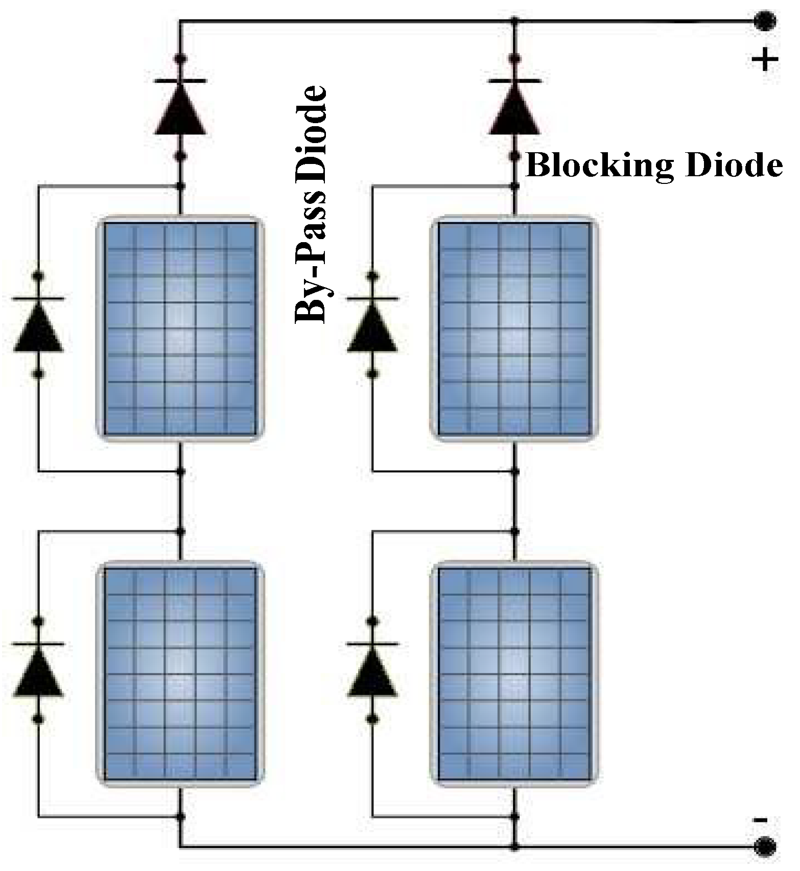
Figure 7 shows a PV array with bypass diodes across each module and blocking diodes at the top of each string. If one of the panels is shaded, it acts as a high resistance and blocks the flow of power produced out of the panel itself and the power produced by the unshaded panel. Hence, a bypass diode comes into play; the current created by the unshaded panel can flow through a bypass diode to avoid the high resistance of the shaded panel. Bypass diodes are not used unless panels are connected in series to generate a higher voltage. Some solar panels are assembled with the cells divided into groups, each with a built-in bypass diode. When the sun shines, the voltage generated by the two panels is more than that of the battery. However, in the dark, the panels produce no voltage [33]. Thus, the voltage would cause a current to pass in the opposite direction through the panels. Hence, blocking diodes prevent the discharge of the battery. Blocking diodes are usually involved in the construction of solar panels. Thus, bypass diodes protect the panels and prevent hot spots in shaded cells connected in series, whereas blocking diodes prevent the reverse current drawn by shaded string [34].

3.2. Far Shading Losses

When the PV array has an elevated horizon, for example, from a nearby mountain range, newly built high skyscrapers, or even city skylines, these objects blackface the sunlight received by the PV array. In such cases, shading from the horizon is applied to the entire PV plant. This happens during the hours in which the sun is below the horizon line. At that time, the array loses its direct irradiance. The energy generated is only based on diffuse solar irradiance. In such events, a solar PV array starts to lose solar irradiance, because Mega objects, such as skyscrapers, are located nearby, from 5 to 15 km. Such losses in a PV plant are known as far shading losses. The designer can model these losses in the PV system by accessing that location’s horizon profile through a simulation. Tools like the Solmetric SunEye or Solar Pathfinder can generate horizon profiles. The Solmetric SunEye is a digital handheld instrument that can be easily carried and used at any project site to capture a far shading profile [35].

In comparison, after capturing the shading profile from the installation site with Solar Pathfinder software, the operator can easily import the shading profile into the system for further analysis. Indeed, the Suneye and Solar Pathfinder are equally efficient and accurate for far shading analysis. Meteonorm and Aurora Solar software can also create the horizon profile remotely based on the online contour mapping facility. Any horizon file that lists the azimuth and elevation angles can model a horizon profile. The line at the bottom of this file is caused by far shading and interpolating linearly. There are two options [36]:

• Losses $\le \mid 1\mid \%$ consider the project site, obtain the horizon profile, and analyze the amount of far shading loss annually.
• Losses $\ge \mid 1\mid \%$ consider changes in the project site, discard the proposed site, or raise the alarm to the management about such losses.

Far shading loss assessment is essential for the proposed project site, as are other parameters, such as cost-effectiveness and accessibility to the local electricity grid [37]. Thus, this impacts the techno-commercial characteristics and long-term economic assessment. Thus, mitigating or optimizing far shading loss is primarily the decision of the project designer.

3.3. Near Shading Losses

These losses occur because of shadows on the solar panel from the objects near it. They can be categorized as

• Nearby obstacles.
  • Nearby buildings, trees, electric poles, and headlines may create shadows on the PV and rooftop installations, such as service areas, water tanks, satellites, and air conditioning chillers. Shade from these obstacles can substantially decrease the PV power plant’s output. Thus, it is recommended that such areas are avoided for installations.
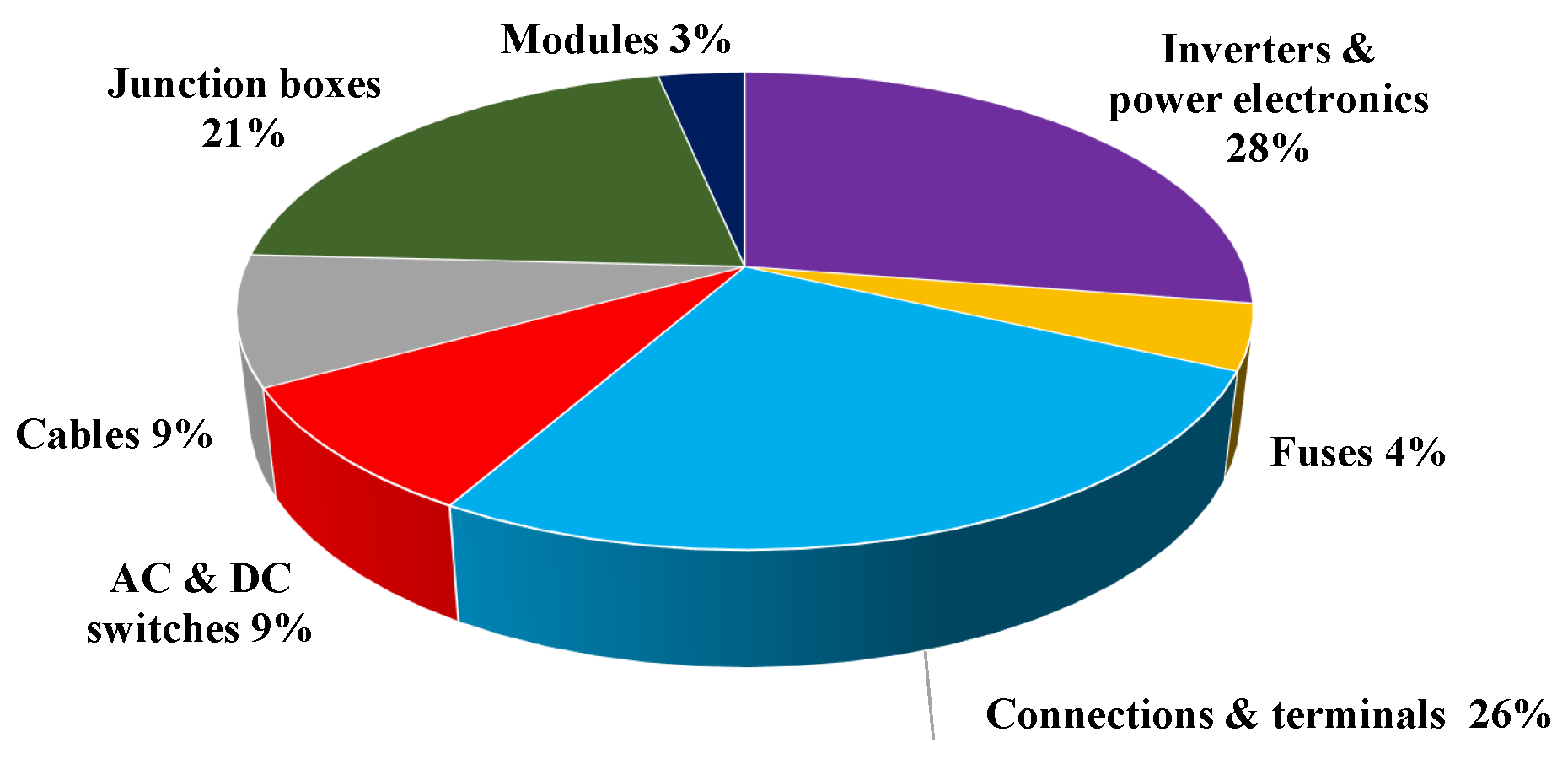
  • Nearby transmission lines passing by the PV site or within the PV power plant can cause shading on the PV module. Similarly, nearby wind turbines may cause a shadow on PV arrays. Shading decreases the total electricity production of PV panels and can create a thermal hotspot, resulting in long-term degradation. Some research states that these shadows cause junction diode failures and fire hazards. Fire accidents can happen in PV installation. More than $80\%$ of these accidents are due to partial shading [38]. Commercially, the manufacturer provides a product and performance warranty for 25 years to 30 years. If the solar panels are installed in the shaded area, the contractual agreement of the module warranty is lost. Figure 8 shows components in which a fire occurred in a PV plant. Table 4 illustrates the potential hazards for firefighters working close to a PV power plant.

Figure 8. Components in which a fire started in 180 PV power plant locations in Germany between 1995 and 2021 [39].

Figure 8. Components in which a fire started in 180 PV power plant locations in Germany between 1995 and 2021 [39].

Table 4. Illustration of potential hazards for firefighters working close to PV power plants [39].

Potential Hazard	Illustration
Electrical shock	Contacting an energized conductor on an energized module or broken energized modules or exposed wires.
Slips and falls	Space limitation.
Collapse	The roof may collapse when support beams are weakened.
Arc or ground fault	An arc may occur from exposed conductors in an energized PV power plant.
Combustion	Materials in the PV power plant may be burnt and release noxious gases.

Table 4. Illustration of potential hazards for firefighters working close to PV power plants [39].

Potential Hazard	Illustration
Electrical shock	Contacting an energized conductor on an energized module or broken energized modules or exposed wires.
Slips and falls	Space limitation.
Collapse	The roof may collapse when support beams are weakened.
Arc or ground fault	An arc may occur from exposed conductors in an energized PV power plant.
Combustion	Materials in the PV power plant may be burnt and release noxious gases.

• Inter-raw shading The insufficient space between the top edges of two mounted strings leads to inter-raw shading. Thus, a specified distance should be kept between the two rows and the tilt angle should be optimized. Hence, an optimized ground coverage ratio (GCR) value should be considered. The GCR is defined as the ratio of the solar PV module area to the overall area of the array. It describes the proportion of the system used to collect sunlight and is calculated by Equation (1).

  $$\mathrm{GCR}={\displaystyle \frac{(\mathrm{N}\mathrm{o}\mathrm{.}\mathrm{o}\mathrm{f} \mathrm{P}\mathrm{V} \mathrm{M}\mathrm{o}\mathrm{d}\mathrm{u}\mathrm{l}\mathrm{e}\mathrm{s})\times (\mathrm{A}\mathrm{r}\mathrm{e}\mathrm{a} \mathrm{o}\mathrm{f} \mathrm{e}\mathrm{a}\mathrm{c}\mathrm{h} \mathrm{m}\mathrm{o}\mathrm{d}\mathrm{u}\mathrm{l}\mathrm{e})}{(\mathrm{T}\mathrm{o}\mathrm{t}\mathrm{a}\mathrm{l} \mathrm{A}\mathrm{r}\mathrm{e}\mathrm{a} \mathrm{o}\mathrm{f} \mathrm{P}\mathrm{V} \mathrm{A}\mathrm{r}\mathrm{r}\mathrm{a}\mathrm{y})}}$$

  (1)
  The GCR provides the percentage of an area that can be utilized for the PV power plant’s installation: the higher the GCR value, the lower the PV capacity. On the other hand, a lower GCR means that the inter-raw pitch is increased, the shading loss is decreased, and the specific PV power plant output is increased.
• Hotspots occur due to junction diode failure; fires may even happen. Finally, an annual near shading loss of up to $\mid 2\mid \%$ is an acceptable limit [40].

3.4. Incidence Angle Modifier (IAM) Losses

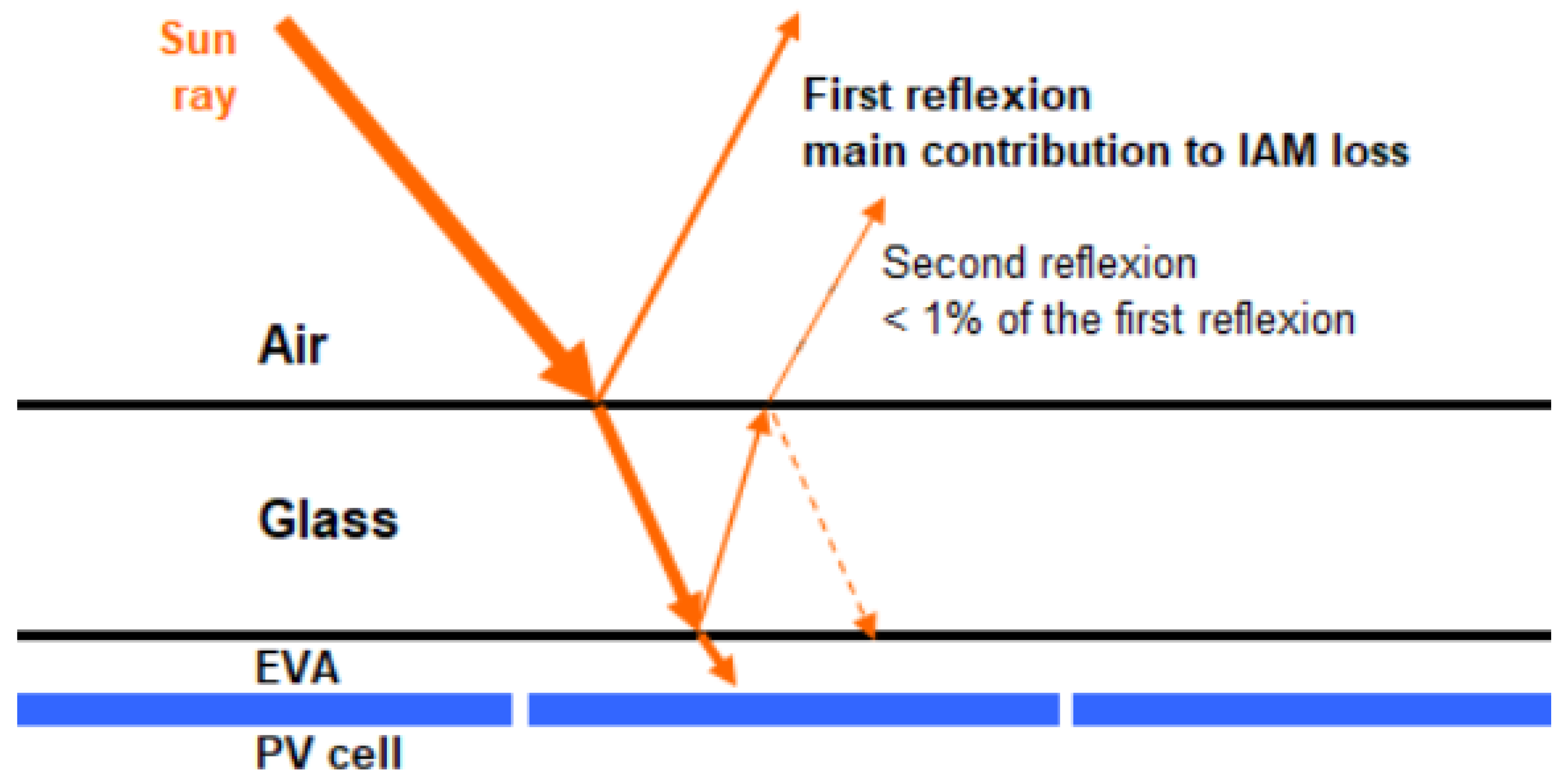
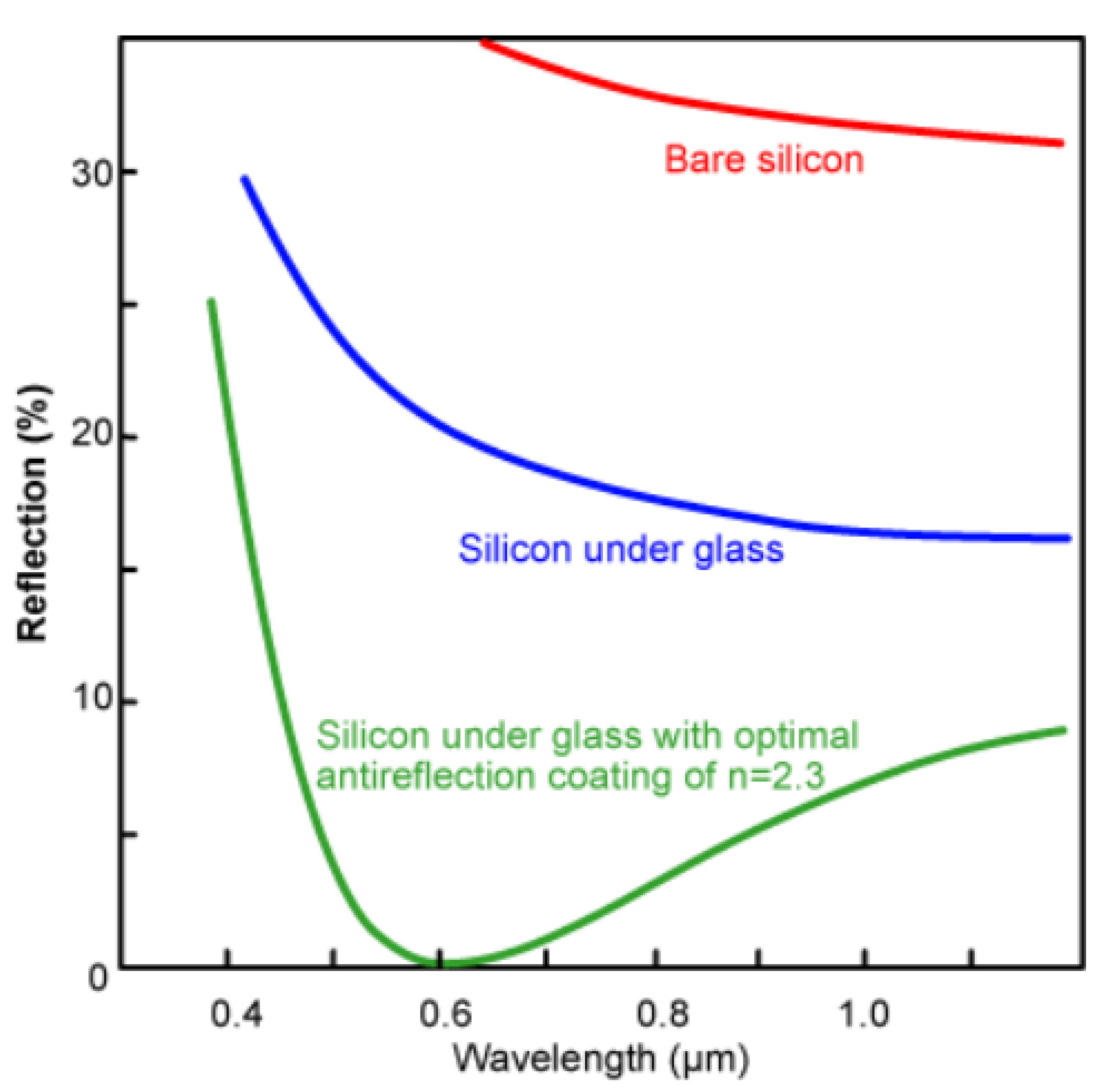
A portion of sunlight is reflected when it strikes the PV module’s surface. The reflection is more significant when the sunlight’s incident angle is high. This reflection loss is technically called the IAM. The PV module consists of different layers, as shown in Figure 9. When sun rays fall on the glass, a portion of the light is transmitted through the layers based on the theory of reflection—Fresnel’s law. If light falls on the glass surface at ${90}^{\circ }$, then the reflection is less than $5\%$ [41].

On the other hand, the reflection is low at a low incidence angle. The IAM applies to both direct and diffuse irradiance. Additionally, solar irradiance is very low during sunrise or sunset. IAM is calculated for each PV module in the array. When the angle of incidence increases, subsequently, the loss effect increases. After ${50}^{\circ }$, the loss starts to grow exponentially [42]. The incidence angle is inversely proportional to the solar azimuth angle. The solution is obtained using the PV modules’ antireflective coating (ARC). The ARC entraps sunlight in a particular medium. Thus, the losses are limited to (2–3%) of the yearly energy yield. Both the glass coating and PV cell surface are manufactured, including the ARC, to reduce the IAM loss. Selecting materials with a high dielectric strength and a specific thickness for ARC film allows most of the sunlight’s bandwidth to be absorbed. Figure 10 shows how PV cells with ARC operate highly efficiently through the various spectra of the sunlight’s wavelength. Major manufacturers provide ARC under standard conditions for all PV modules [43].

Figure 9. IAM–PV array incidence loss [44].

Figure 9. IAM–PV array incidence loss [44].

The IAM optical loss factor is given by Equation (2) [45]:

$$IA{M}_B=\frac{\tau \left(\theta \right)}{\tau \left(0\right)}=\frac{R\left(\theta \right)-A\left(\theta \right)}{R\left(0\right)-A\left(0\right)}$$

(2)

where $\tau$ is the weighted transmittance, R is the weighted reflectance, and A is the absorbance. The weight of the IAM loss factor is calculated using the spectral distribution of radiation and the PV module spectrum response. The basic approach for describing the IAM was developed by Souka and Safat in 1966 [45]. The American Society of heating, refrigeration, and air conditioning (ASHRAE) developed the model. The new model is given by Equation (3) [46].

$$IA{M}_B=1-b_0\left(\frac{1}{cos\left({\theta }_{AOI}\right)}-1\right)$$

(3)

where AOI is the angle of incidence. Equation (3) has a discontinuity problem at ${\theta }_{AOI}=90$, whereby it is inaccurate at low incident angles [46]. Another IAM model was adopted in 2006 by De Soto, based on Snell’s and Bougher’s law. In this model, the angle of reflection $\left({\theta }_r\right)$ is given by Equation (17) [47]:

$${\theta }_r=arcsin\frac{l}{n}sin\left(\theta \right)$$

(4)

where l is the index of reflection of the air, n is the index of reflection of the cover glass, and $\theta$ is the angle of IAM. $IA{M}_B$ is given as shown in Equation (18) [47]:

$$IA{M}_B=\frac{\tau \left(\theta \right)}{\tau \left(0\right)}$$

(5)

where $\tau \left(\theta \right)$ is the transmittance at angle $\theta$ and $\tau \left(0\right)$ is the transmittance normal to the sun. $\tau \left(\theta \right)$ and $\tau \left(0\right)$ are given by Equations (6) and (7), respectively [47].

$$\tau \left(\theta \right)=e^{\left(\frac{KL}{cos\left({\theta }_r\right)}\right)}\left[1-\frac{1}{2}\left(\frac{si{n}^2({\theta }_r-\theta )}{si{n}^2({\theta }_r+\theta )}+\frac{ta{n}^2({\theta }_r-\theta )}{ta{n}^2({\theta }_r+\theta )}\right)\right]$$

(6)

$$\tau \left(0\right)=\underset{\theta \to 0}{lim}\tau \left(\theta \right)=ex{p}^{-KL}\left[1-{\left(\frac{1-n}{1+n}\right)}^2\right]$$

(7)

The typical parameters for the PV module are as follows: n (refractive index) = 1.526 (glass), K (glazing extinction coefficient) = 4 m${}^{-1}$, and L (thickness of transparent cover) = 0.002 m [47]. Additionally, there are Sandia IAM models that describe these losses as a 5th-order polynomial [48] and the Martin and Ruiz IAM model [49,50,51].

3.5. Soiling Losses

These are caused by the accumulation of snow, dirt, dust, leaves, pollen, and bird droppings on PV panels. Thus, the accumulation of soil on the PV module can lead to a significant decrease in energy production by the PV module [52,53]. The amount of sunlight blocked by dirt and debris accumulates on the solar panels over time. Soiling losses are not constant throughout the year. They depend on weather and season changes. The driving factors for the soiling losses are as follows [54]:

• Locations vary from region to region. The soiling loss profile differs between Europe and the gulf region. There are more dust particles in the gulf region air than in other places due to the deserts.
• Air pollution is not the same everywhere. It is near industrial, dense urban, and corp land. In the agricultural area and during the season of corp harvesting, the soiling rate increases rapidly. However, for the rest of the year, it remains deficient. The percentage loss due to dust decomposition is higher than in other places, especially in suburban areas where many public and private means of transport move around on the road daily.
• Air mist: A higher moisture content makes dust stick to surfaces. Thus, the dust remains stuck to the surface, even with heavy wind.
• Bird droppings: Forced cleaning is required to remove the deposition. This represents a severe problem; the rain does not remove them. Nevertheless, their reported impact is relatively small ≤2% in terms of the total soiling loss.
• Snow: Heavy snowfall covers entire PV arrays. The whole modules are cut off from sunlight, and there is no electricity production. However, if the module surface is partially covered by snow, it is hazardous, as it causes electrical damage to the PV module.

The soiling loss (SL) values observed from many solar plants throughout the world in recent years are as follows [55]:

• +(1–5)% if the region experiences frequent dust deposits.
• +(1–2)% if the region is near major vehicular traffic areas.
• 0.5% if the system is cleaned in summer.

The solutions to reducing the soiling loss are as follows [4]:

• Clean the PV surface regularly with a 15–30 day cycle for large systems and every 60–90 days for small rooftops.
• Table 5. PV power plant cleaning methods [57].

  Method	Illustration
  Natural	Wind, gravitation, snow, rainfall.
  Manual	Washing using certain fluids, surfactants (detergents), clothes, and brushing.
  Mechanical	Brushing, blowing, vibrating ultrasonic, diving.
  Self-cleaning	Electric charge, surface covered with a pellucid nanofilm.

  shows different cleaning methods used in PV solar systems.
• Higher tilt angles help to remove dust naturally. It is recommended that the tilt angle is low for installation. The tilt angle depends on the location and time of the year [56].

The average number of days between cleaning events (n) in the PV power plant is given in Equation (8) [58]:

$$n=\frac{365}{C_{optimum}}$$

(8)

where $C_{optimum}$ is the optimal number of cleaning cycles, and the increment of $S_{loss}$ per day is known as the soiling rate (SR). For instance, a SR of $0.2\%$/day means that the $S_{loss}$ is $0.2\%$ for the first day. Then, it increases to $0.4\%$ and $0.6\%$ for the second and third days, respectively, and so on. Thus, the $S_{loss}$ is given by Equation (9) [58].

$$S_{loss}=\sum _{k=1}^{n}k\times SR=SR\frac{n^2+n}{2}$$

(9)

where k is the number of days with no cleaning. The annual yield loss $Y_{loss}$ is given as shown in Equation (10) [58].

$$Y_{loss}=C\times Y_{\mathit{spec}}\times C_{\mathit{optimum}}=365C\times Y_{\mathit{spec}}\times SR\times \frac{n+1}{2}$$

(10)

where C is the installed capacity of the PV power plant, and $Y_{spec}$ is the specific annual yield.

3.6. Potential Induced Degradation (PID) Losses

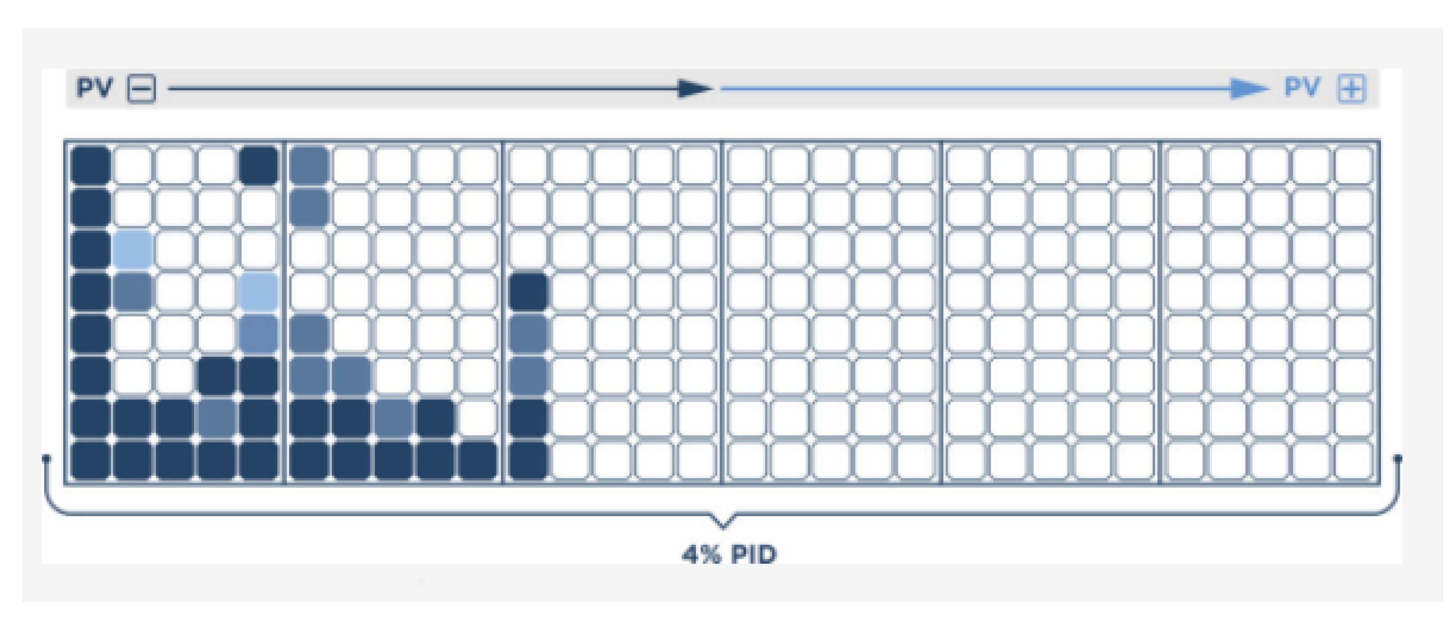
The solar panel consists of individual PV cells. Each of these cells generates electricity from the collected sunlight. These solar cells are large photodiodes where the charge currents are separated due to the PN junction’s electric field. The incident sunlight dislodges electrons. These electrons then flow along with the contacts and generate green electricity. The grounded PV array has a string or array grounding, so the potential across the system always remains positive to the Earth. PID does not occur in grounded systems, where the inverter’s negative pole is grounded, or in systems less than or equal to 600 V. Here, eliminating the high negative voltage potential drives the PID phenomena. Thus, the potential can float between high positive or negative values in an ungrounded PV array. The high voltage difference across the solar module structure is responsible for degradation. Due to the high negative potential to the Earth, sodium ions from glass are ionized and drift toward the solar cell. These Na${}^{+}$. ions penetrate through the arc layer to the emitter layer of the solar cell, and electrons captured by Na${}^{+}$ ions become Na. The high relative voltage forces the sodium ions to diffuse from the glass through encapsulation and eventually accumulate on the cell surface. Modules with negative potential concerning the ground are mostly affected.

The PID affects panels closer to the string’s negative side. The negative potential concerning the Earth is the highest on that side. In an individual PV module, the PID effect is more potent in cells closer to the aluminum frame, whereas it is less effective in cells in the center of the modules. Figure 11 shows that the PID affects solar modules near the negative string more. Currently, the system level exists due to higher string voltage designs, such as those with up to 1500 V, which can create a very high potential difference and a transformerless inverter (floating potential) [8].

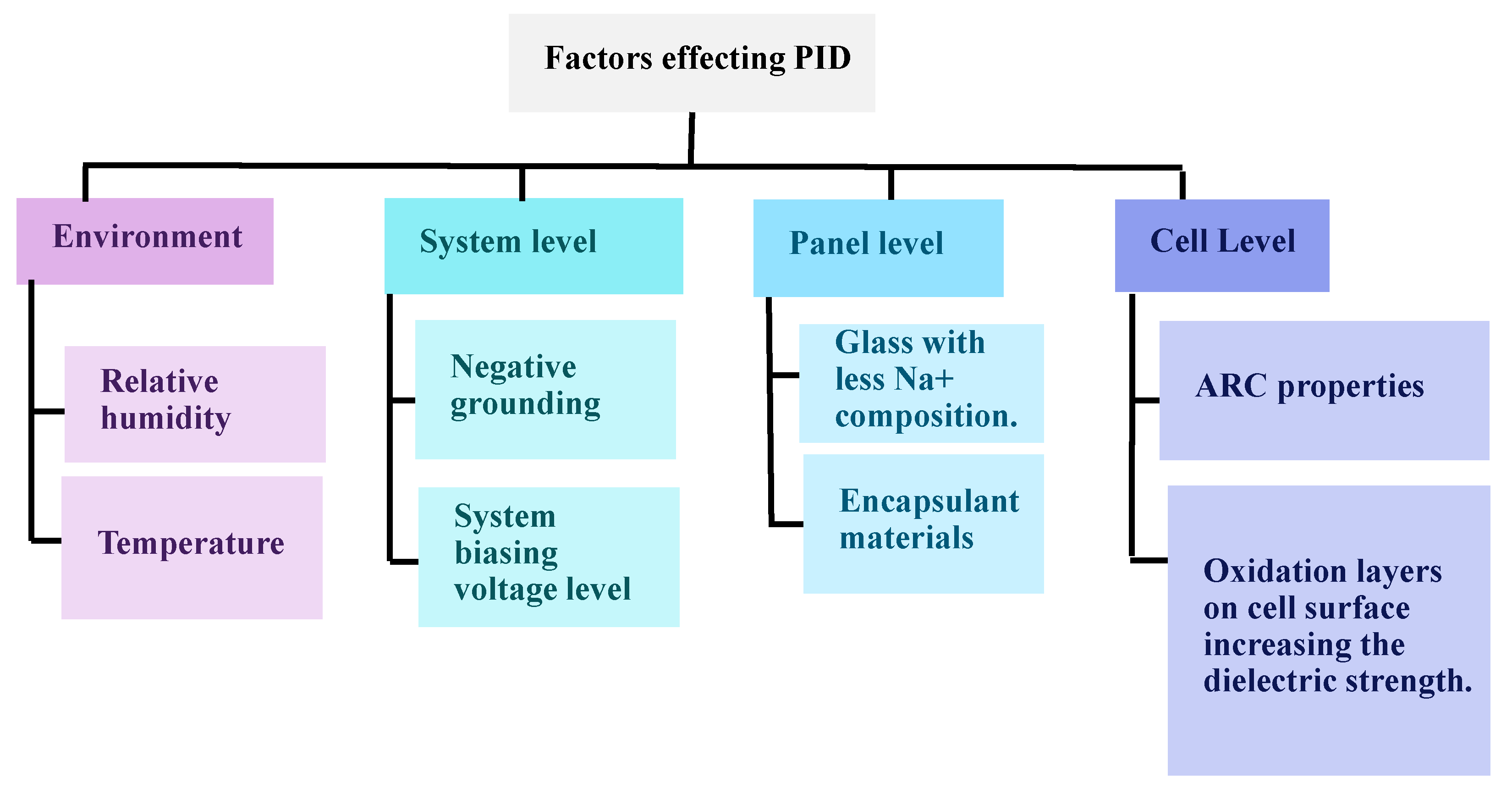
Figure 12 shows three levels of strategy under control (plant, panel, cell) and the environmental factors that can not be controlled. The PV module’s PID process may overgrow and affect the entire PV plant’s performance in the shortest period. Consequently, this results in damage to the PV’s plant financing and operation. PID can be prevented and reduced at the plant level. Humidity and temperature influence the leakage current in conjugation with the voltage level in the installation determined by the module connection scheme and solar irradiation. The leakage current peaks during morning hours when the modules’ faces are covered with morning dew [59].

This process creates a stacking fault through the solar cell. It happens at the microcrack surface, increasing recombination and reducing the power output—the propagation of microcracks when walking on a PV module. When the mechanical load is released, these cracks become invisible. The occurrence of microcracks reduce the performance and causes a direct financial loss.These cracks also occur during transportation, installation, and operation. Most breakage locations that occur during module design and construction after mechanical stress tests are located in the module’s center. It is due to being the area of the highest mechanical tension and stress by bowing [60,61].

Power reduction caused by the PID may happen gradually over time or immediately after installation. Power loss $\Delta P$ is proportional to current loss through the equivalent PV cell circuit shunt. PID is responsible for power losses of up to $30\%$. This mechanism has become very important due to the high PV voltage rating. PID can affect the modules within a few years and decrease the PV modules’ output power. More work has been done on developing a PID sensor to detect PID before a $1\%$ power loss occurs. The detection device’s operation is based on the electrical quantity, which is easy to measure. Usually, the installation site’s modules are removed and tested indoors. This action is considered time-consuming and costly and causes damage to the modules. Yield and efficiency are lost in a PV power system every day. The result is a dramatic loss of earnings within a short period of time. Polarization and leakage currents in the module cause these losses. Solar cells become inactive. Finding a PID killer increases the PV array to a highly positive potential and reversing the polarization effect is considered an open research problem. In a few months or years, the performance could deteriorate by $30\%$ to $40\%$ or more. PID accelerates performance degradation, which grows exponentially. An early detection mechanism for PID is essential, because it allows for some reversal of that effect. Prevention is always preferable to treatment. According to Finsterle, PID lowers the open-circuit voltage $\left(V_{oc}\right)$ and the module’s maximum power point (MPP) [62].

PID is considered one of the crucial factors associated with PV reliability. PID testing comprises a 96-hour test period, during which test panels are subjected to humidity and temperature levels of $85\%$$(\pm 5\%)$ and $60{}^{\circ }$C ($\pm 2{}^{\circ }$C), respectively. The voltages applied to these panels may correspond to the maximum plant voltage listed in the panel datasheet. The IV measurement is visually inspected as part of the PID testing method. The module must pass the test without significant defects and with a power loss not exceeding $5\%$. PID increases the probability of not guaranteeing a 25-year warranty life. Additionally, high humidities and temperatures cause more significant overall losses. At an early stage, PID can be reversed by changing the voltage bias. PID is not detectable to the naked eye. Tests can be used to sense PID in operational sites such as thermal images, electroluminescence, and IV curves. PID can be prevented using strings with isolation transformers between the strings and the inverters, negative terminal grounding, and installation of the anti-PID [62].

3.7. Temperature Losses

A fraction of solar cell radiation produces electricity, and the remaining radiation is converted into thermal energy. A portion of the produced thermal energy increases the solar cell’s temperature, dissipating the rest from the top and bottom of the cell. The temperature of the cell determines its electrical performance. Hence, the IV curve in the PV module at a given irradiance states that the power output decreases when the temperature increases and there is a voltage drop. In comparison, the PV solar output power is increased when the temperature falls while the irradiance remains constant [11]. Conveniently, a semiconductor demonstrates better conductivity with an increasing temperature, and at zero Kelvin, it acts as an insulator. This can be explained by Equation (11). The net effect of temperature is linearly related to the open-circuit voltage $V_{oc}$, while the temperature is associated with the rise in the photodiode’s leakage currents. The cells with lower $V_{oc}$ are more affected by temperature than cells with higher $V_{oc}$. This implies that a solar cell based on crystalline silicon with $V_{oc}$ of 650 mV is more affected than an amorphous silicon solar cell with an $V_{oc}$ of 850 mV [63,64].

$$V_{oc}=\frac{kT}{q}ln\left(\frac{I_{ph}}{I_o}+1\right)$$

(11)

Fabrication of the PV module includes the temperature coefficients in the commercial modules’ datasheet. The temperature coefficient of power is the rate of change in the output power concerning the temperature. Likewise, the temperature coefficient is the rate of change in a voltage concerning temperature. A typical datasheet of a commercial module specifies temperature coefficients for the $I_{sc}$, $V_{oc}$, and power under STC. Equation (12) shows how to calculate the PV power output concerning the temperature change $\frac{dP}{dT}$. The reference temperature $25{}^{\circ }$C is considered to be the STC temperature [63].

$$P\left(T\right)=P_{STC}+\frac{dP}{dT}\times \left(T-T_{STC}\right)$$

(12)

The operator should distinguish between the module temperature and ambient temperature. The difference in heat flow in and out of the module’s encapsulation solar cells is affected by various factors. The primary factor involved in increasing the PV module’s operating temperature is the thermal equilibrium between the heat lost to the surrounding environment and the PV module’s heat. Heat exchange with the surroundings depends on the heat transfer coefficient of the module and its surface area, wind speed, and ambient temperature. The conductive heat loss is caused by heat flow from one material to another. The NOCT model is expressed in Equation (13), where the cell temperature depends on the irradiance and the ambient temperature [65]. Thus, the cell temperature never goes below the ambient temperature, and the minimum limit is at the ambient temperature. It takes place at night when the irradiance is zero. The NOCT of a particular PV module depends on the nominal wind speed of 1 m/s, an ambient temperature of $20{}^{\circ }$C, the PV cell under an irradiance of 800 W/m${}^2$, and the no-load conditions (${\eta }_c=0$). The performance of the module is worse due to the temperature effects that drop the PV output power at high cell temperatures while the sun shines in summer [63,66].

$$T_{cell}=T_{ambient}+G\times \frac{NOCT-20{}^{\circ }\mathrm{C}}{800{\mathrm{W}/\mathrm{m}}^2}$$

(13)

In addition, the energy balance is given in Equation (14) [63,66]:

$$\alpha \tau I\left(t\right)={\eta }_{c}I\left(t\right)+U_L(T_{cell}-T_{ambient})$$

(14)

where $\tau$ is the transmissivity of the cover of the solar cell, $\alpha$ is the absorptivity of the solar cell, ${\eta }_c$ is the electrical efficiency, $I\left(t\right)$ is the PV output current (A), $U_L$ is the overall loss coefficient, and $T_{cell}$ is the solar cell temperature. For no-load conditions, ${\eta }_c=0$. Thus, Equation (14) can be rewritten as Equation (15) [63,66].

$$\frac{\alpha \tau }{U_L}=\frac{T_{cell,NOCT}-T_{ambient}}{I{\left(t\right)}_{NOCT}}$$

(15)

Thus, the cell temperature can be found with Equation (16)

$$T_{cell,NOCT}=T_{ambient}+\frac{\alpha \tau }{U_L}I{\left(t\right)}_{NOCT}$$

(16)

3.8. Light-Induced Degradation (LID) Losses

Some modules experience a permanent blackout in power output upon initial exposure to light. Thus, the efficiency is reduced. The degradation ranges from $1\%$ up to $5\%$. Hence, LID phenomena play an essential role in manufacturing a-Si-based solar panels. Amorphous silicon (a-Si) has been the best-developed thin-film material in commercial production since 1980. It is an inexpensive material [67]. Its amorphous nature has several significant consequences for PV. Here, the shedding light’s absorption is acceptable, but doping and charging transportation are difficult.

In 1977, it was discovered by Staebler-Wronski that there are dangling bonds of different lengths and orientations in amorphous silicon (Si) materials. When the conductivity of a-Si is exposed to light for a specific period of time, the conductivity drops to a certain level based on the a-Si phenomenon. There are many models to explain this observed behavior. One of these models is the hydrogen bond switching model. This model supposes that the silicon items are bonded in the a-Si. When light shines on this material, electrons are generated in whole pairs. These electrons and hole pairs are virtually connected. They can recombine and release a photon from the bond. This energy breaks the bond and releases the energy. This is essential to create the dangling bond on these silicon atoms. Briefly, this model states that this bond is essentially switched by hydrogen. This hydrogen is present in a-Si materials. The bonds between the two silicon atoms and hydrogen represent H-bond switching. The dangling bond’s density increases as light shines, because of the recombination of these electron and hole pairs that are generated as a consequence, as well as due to the creation of dangling bond states [10].

Another model is the hydrogen-collision model. In this model, dangling bonds are created in these amorphous materials. Silicon items are bonded to hydrogen. When light shines, it causes these bonds to break, creating dangling bonds on each silicon atom. The hydrogen is subsequently set free and released [68].

3.9. PV Yearly Degradation Losses

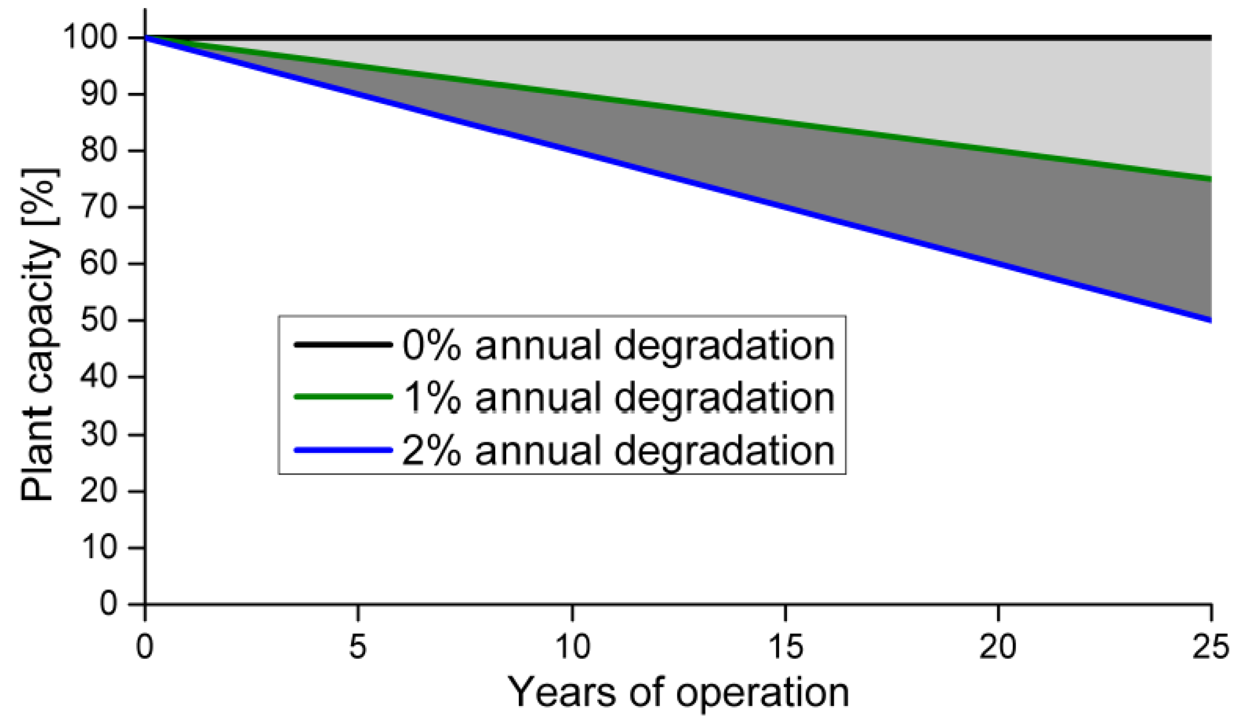
The PV module’s performance is generally rated under STC: an irradiance of 1000 W/m${}^2$, a solar spectrum of AM 1.5, and a module temperature at $25{}^{\circ }$C. The module’s actual $V_{PV}$ and $I_{PV}$ change as the lighting temperature and load conditions change. The module’s performance depends on the time delay, solar installation, direction and tilt modules, cloud cover, shading, temperature, geographic location, and day. The voltage and current fluctuations are logged with a multimeter or data logger. More complex and high-efficiency technologies have higher potential for degradation. Figure 13 shows the drop in the plant’s output capacity for three annual degradation cases. Three key factors were used as the selection criteria: reliability, technology selection, and the levelized cost of electricity (LCOE). Technology selection depends on the insulation, temperature, precipitation, and geography. The module’s performance was simulated based on actual weather data. LCOE describes the cost of power produced by a PV power plant over time, typically the plant’s warranted life. The most significant impact of LCOE is the cost of PV modules, as they constitute the central part of the plant. Many factors impact the LCOE cost, such as the module price, the power generated by a module over its warranted life, and the power degradation during a module’s lifetime [12].

3.10. Array Mismatch Losses

Array mismatch losses occur when solar panels of different wattages and voltages or manufactured by different companies are mixed. However, these are not recommended or prohibited. In this case, particular interest should be given to each panel’s electrical parameters. When two panels from different vendors are connected, the problem is that they have different electrical characteristics and, thus, various degradation performances. Wiring mismatched solar panels together negatively impacts the solar output power. Operators should take a look at the parameters on both panels. Therefore, a datasheet is available on the back of the panels; the operator should pay more attention to $V_{oc}$, $V_{mp}$, $I_{sc}$, and $I_{mp}$. The ideal cell would have a perfect rectangular characteristic, and the closeness of the characteristics to the rectangular shape is a measure of the cell’s quality. The solar cell’s output power increases with solar radiation. The $I_{sc}$ changes are essentially proportional to the change in solar radiation. However, the voltage difference is comparatively less. However, there are a few drawbacks. The operators should use the maximum power point (MPPT) and charge controller to absorb the excess voltage and bring it down to the battery bank [70,71].

The least-rated power module determines the overall rated current in solar modules connected in series and drags the overall plant output down. The overall voltage should not exceed the maximum voltage limit of the MPPT charge controller connected to the modules [72,73]. While modules connected in parallel obtain a high current, the voltage is the lowest with parallel connections. The current in a series connection and the voltage in a parallel connection decrease the solar array’s performance. Reducing the current or reducing the voltage of one of the panels reduces the power output, therefore causing a reduction in the system’s performance. Hence, wiring mismatched solar panels together negatively impact the solar power output. As the operator adds many panels, the wire size should be increased [13,14]. In some cases, the underperformance of a module could have a cause as small as a crack in the module, the soiling conditions, or the presence of some hydraulic fluid in the construction process, all of which have the same effect as the mismatched module [74].

3.11. Module Quality Losses

Understanding the quality of PV components and translating this information into actionable results is more important than ever. A healthy PV power plant mainly depends on the reliability of its components. Hence, the module’s quality depends on performance and safety issues associated with its assets. The detection of module degradation is based on many issues, such as thermal anomalies, often giving modules a sense of power loss. This information is combined with electrical factors at the string or panel levels, giving further information about gradual losses in historical power data analysis. Historical degradation by inspecting the power data is considered an important issue. It can shed light on quantitative historical losses and trends. Combining this visual inspection and laboratory analysis can determine and confirm the nature of degradation and safety risks. IV measurements can quantify gradual losses compared with power nameplates. Each year, amassed field inspection information and data are gathered and analyzed [75,76].

Defect modules can be classified into cell and interconnection types, such as corrosion, hot spots, snail trails, broken interconnections, cracks, and burn marks. Additionally, a back sheet includes the outer layer (airside) and the inner layer (cell side), cracking, delamination, and yellowing. Encapsulants include discoloration, browning, and delamination. Different defects include glass defects, a loss of the antireflection coating (ARC), and junction boxes. The long-term performance is affected by field failures. Many modules may not be able to last 20–30 years. Statistics show an increment in the field’s frequency and extent of module and plant failures. All modules are not created equal in terms of new cells, technologies, and materials. They support the worldwide PV community by generating data that accelerates solar technology adoption. Quality testing shows many common solar panel defects, such as scratches and uneven or excessive glue on glass and frames. Unsealing problems exist, such as gaps between the glass and the frame. Thus, the output or fill factor is lower than stated in the datasheet, and the cell colors and alignments are inconsistent. Figure 14 shows some of the PV modules’ quality losses [77].

4. Electrical Losses

Electrical losses in PV solar systems include cable, inverter, transformer, and transmission line losses. These losses can also be classified as DC plant losses, AC plant losses, and DC to AC conversion losses.

4.1. DC & AC Cable Losses

Most solar power kits or packages do not come with wire. The installer is responsible for the wires and cables needed for their installation. They do this because every installation is unique, and the preference is to keep the package price low. The enormous challenge of wire choice depends on the budget and project. An understanding of wiring materials and diagram is needed to make the correct purchase decision for a PV solar system [19].

• There are many types of wire, which can get confusing. Wires differ in terms of the conductor material’s insulation and flexibility. The most popular and widely used conductor for solar applications is pure copper. Aluminum is another option. It is relatively cheaper than copper. Wires can come with various insulation types that vary in terms of their protective properties. Some work better in high temperatures, high moisture conditions, under high UV exposure, or when exposed to fire than others for indoor solar wiring, such as in sheds or garages. The wire can have a solid core construction or standard, so it is flexible. Standard wire offers a greater surface area for flow and thus delivers better conductivity than solid cores. In most cases, it is best to use standard wire for PV solar systems.
• The wire’s thickness and length determine how much current can be safely carried. A PV designer or electrical engineer can find the economically optimal wire size.

There is massive investment in solar panels, inverters, charge controllers, mounting equipment, and batteries in PV solar systems. The plant is at risk if one chooses the wrong excess carrying capacity for wires. One of these risks is the friction effect. Overloading occurs when the current increases and more thermal energy dissipates. Thus, the operational temperature of the insulation and the wire rise beyond a specific limit. In some cases, voltage loss causes equipment failure or malfunction [78]. More panels can be added to the system and rewired at some points. The cables should meet weather and UV resistance requirements, withstand an operating temperature range of $-40{}^{\circ }$C to $+125{}^{\circ }$C, and withstand the voltage, depending on the application. Flame-retardant, halogen-free insulation, and sheath properties are considered self-extinguishing as well as acid- and alkaline-resistant characteristics. Cables should maintain short circuit resistance at high temperatures of $250{}^{\circ }$C. It is preferable to have a small diameter to save space and allow the wire to be abrasion-resistant and have a high mechanical strength. PV cable installation should take as little time as possible to minimize the DC voltage drop and reduce the magnetic field’s susceptibility [79].

Most of these losses are design issues, while none are stable—they vary according to the load conditions. Correct design and sizing of the cables, as well as regular electrical maintenance, are the main ways to combat DC and AC cable losses. They are impacted by choosing the right components and installing cable runs with suitable cross-section areas.

4.2. Inverter Losses

Inverters in PV solar systems mainly determine the functionality, for example, the static and transient characteristics, performance, and reliability. These inverters’ essential functions are DC–AC conversion, MPPT, current grid control, active anti-islanding, and various monitoring and protection requirements. The trend nowadays is to use smart inverters with grid support features. Inverters are classified as grid-connected and stand-alone, single-phase, or three-phase. Concerning transformer isolation, inverters can be classified based on their line frequency, for example, high-frequency transformer or transformerless intervers [80].

Inverters can be classified as central, string, micro, and multistring inverters.

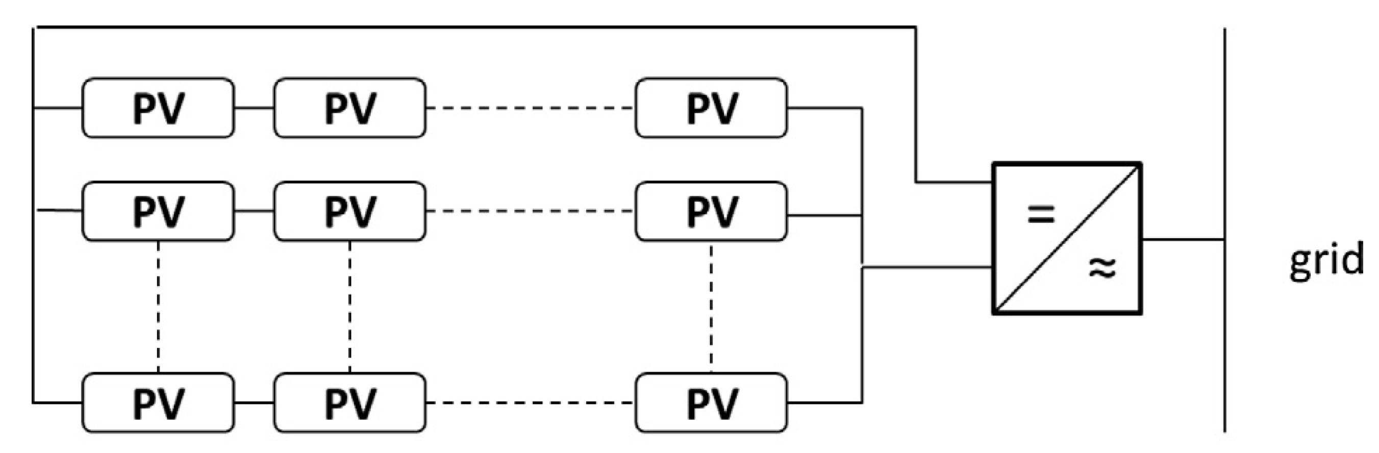
• Central inverters are used in large-scale applications, as shown in Figure 15. Their peak efficiency is around $98\%$. They have some problems due to a mismatch between modules and strings. A loss of single inverters leads to the entire or a large part of the power generation being lost.
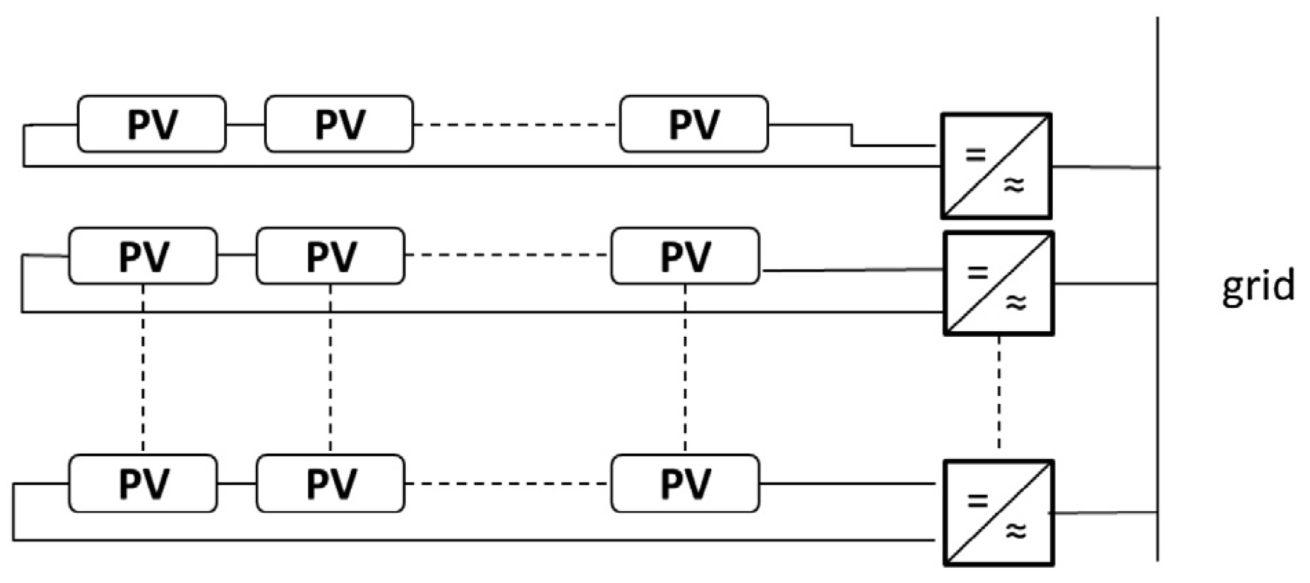
• String inverter systems are used in residential applications, ranging from 2 kW to 6 kW, as shown in Figure 16. In this inverter type, there are multiple strings with individual inverters as possible configurations. String-level MPPTs are better than nonoptimal central inverters.
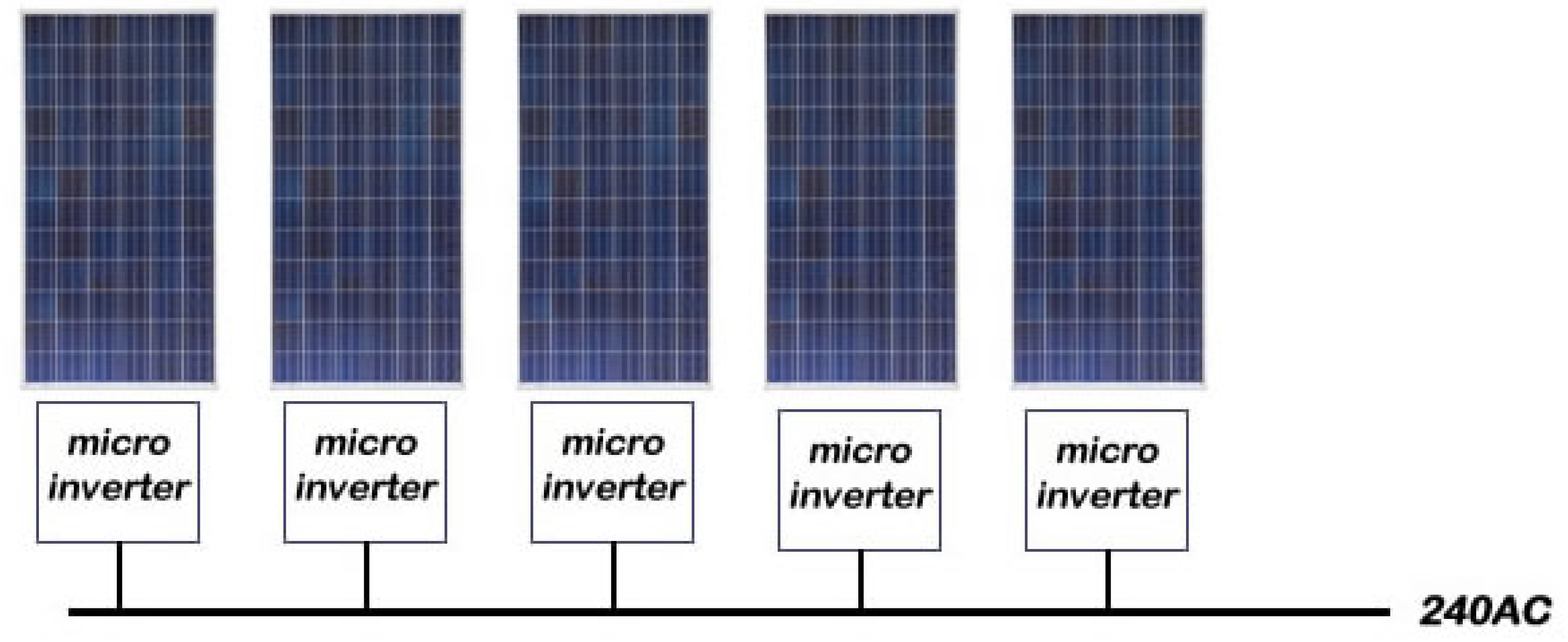
• Microinverters are used in applications requiring less than than 500 W. They are mounted at the back of the panel with one per panel. There is a direct connection to the single-phase grid through AC wiring, as shown in Figure 17. Concerning MPPT, there is a higher energy yield than string converters, especially when significant shading is expected. This type requires the elimination of high-voltage and high-current DC switches and wiring.
• Multi-string inverters combine the higher energy yield of a string inverter with the central inverter’s. Each string has its MPPT implemented alongside the DC-DC converter.

Choosing a suitable inverter depends on the overall power system’s size. These converters are connected via a DC bus to the inverter and, ultimately, to the grid. A new string with a dedicated DC-DC converter must be included within a specific power range to expand the system’s size. Central and string inverters require less labor hours and are more affordable than microinverters. Additionally, they need fewer connections through cables than microinverters. However, microinverters can undergo rapid shutdown. There is no doubt that inverters are the most sophisticated devices in the PV solar system, despite their high failure rate compared to other system devices.

Table 6. The main pros and cons of the topologies of inverters used in PV solar systems.

Topology	Pros	Cons
Central	Initial investment, maintenance, design, and implementation.	DC wiring cost, shading performance loss.
String	Performance loss mitigation.	Design and implementation, initial investment, maintenance.
Micro	Performance loss mitigation, DC wiring cost, design.	Initial investment, maintenance.
Multistring	Performance loss mitigation, initial investment.	Design and implementation, maintenance.

shows the pros and cons of the topologies of inverters used in PV solar systems.

Figure 15. Configuration of the PV central inverter [81].

Figure 15. Configuration of the PV central inverter [81].

Figure 16. Configuration of the PV string inverter [81].

Figure 16. Configuration of the PV string inverter [81].

Figure 17. Configuration of the PV micro inverter [81].

Figure 17. Configuration of the PV micro inverter [81].

Stand-alone PV solar systems are mainly used for DC loads, such as mobile applications, street lamps, signs, telephones, and water pumps connected to DC motors. On the other hand, stand-alone AC loads are used in remote or off-grid applications because it is not economical to extend the power grid. These systems are used in complete solar homes with conventional AC loads, such as water pumping applications. Grid-connected solar PV systems mostly uses central inverters and they have applications in systems ranging from 250 kW up to 1 MW. Typically, large PV solar plants have several MW scale inverters. The topology choice for implementation depends entirely on the system’s needs, size, and budget. The inverter choice for a PV system depends on the inverter’s characteristics, and the inverter should be as efficient as possible. Thus, it must deliver maximum amount of PV-generated power to the grid or load.

Under rated conditions, the typical efficiency is more than $95\%$. An active islanding detection capability is essential for grid-tied inverters. Islanding means that the inverters in a grid-tied setup continue to power the system even though the grid operator’s power is limited. Islanding needs to be prohibited due to safety issues. Therefore, inverters are expected to respond and detect by immediately introducing power to the grid. This is referred to as anti-islanding. In many situations, solar inverters are exposed to ambient conditions. They must comply with the location’s temperature and humidity conditions, since grid-tied inverters pump power into the grid. A high quality must be maintained to prevent the disruption of the grid’s power flow. Thus, inverters are expected to have a low harmonic content on the line currents. This increases the lifespan of the inverter, the crucial power electronic device in modern PV systems. A suitable inverter is probably attained under favorable conditions with a lifetime of around 10–12 years. The modules in a PV system can last for over 25 years [82].

There is no benefit in harvesting energy from solar arrays during low insulation and low-light periods (early day, late day, cloudy day). Inverters convert a fraction of the virtually offered energy. The use of high-performance power electronics (HPPE) double conversion was recently attempted [83] to maximize the system’s efficiency and therefore its profitability. Many factors should be considered when estimating inverters, such as the electrical yield (kWh/kW), inverter’s lifespan and warranty, modularity, indoor vs. outdoor installation, considerations inside the cabinet, high and low ambient temperatures, and transformer isolation [84].

The decent cooling of PV solar system inverters is an essential criterion to guarantee the reliability of their operation. If the junction temperature of switching devices exceeds the limits, the devices fail. Heat sinks are used to remove the dissipated power in switching devices. Thus, an adequate heat sink needs to be chosen for a particular application. It is necessary to estimate the power dissipation in the switching device. The ideal switches have zero ON-state drops and, hence, no conduction losses, zero leakage current, and no OFF-state loss. Additionally, turn-ON and turn-OFF transitions are instantaneous, and there is no energy loss during switching transitions [85]. In comparison, practical losses are finite forward drops and conduction losses as well as finite turn-ON and turn-OFF transition times. The transition between switch states is instantaneous, and the voltage drop across the conducting throws is zero.

Power losses in an inverter can be expressed as shown in Equation (17).

$$P_{AC}=P_{DC}-P_{conduction}-P_{switching}-P_{stray}$$

(17)

The switching energy loss is calculated based on the IGBT turn-ON energy loss $\left(E_{ON}\right)$ as a function of the DC voltage, current, and junction temperature and the IGBT turn-OFF energy loss $\left(E_{OFF}\right)$ as a function of the DC voltage, current, and junction temperature. They are available in the IGBT datasheets for various operating and environmental conditions. The calculation of inverter switching is based on having a constant DC bus voltage, $E_{ON}$, and $E_{OFF}$ that vary with the load current. Additionally, the ripple in currents is neglected. The variation in the switching energy loss with current can be approximated by a simple function (linear, piecewise linear, or parabolic). Thus, the switching loss is the product of the average switching energy loss and the switching frequency. Losses are calculated based on how much current passes through the switch. Each switch has a DC input and an AC output voltage to characterize inverter losses and correlate them to obtain precise efficiency measurements. The resistance of each switch is estimated with a time-aligned temperature. The average conduction loss in a power semiconductor device depends on the switch and connection resistances [83]. It can be calculated using the following Equation (18)

$$P_{conduction}=I_{on}\left(avg\right)V_{on}+I_{on}^2\left(rms\right)R_{on}$$

(18)

where $I_{on}\left(avg\right)$ and $I_{on}\left(rms\right)$ are the average and rms conduction state currents, respectively. They can be determined from the converter’s operating conditions. $V_{ON}$ and $R_{ON}$ are the ON-state forward voltage drop of the device and the ON-state resistance of the switching device. It should be noted that MOSFET does not have $V_{ON}$, and other devices have negligible $R_{ON}$ [82] The turn-OFF loss can be expressed by Equation (19)

$$P_{OFF}=\frac{1}{2}{V}_{OFF}{I}_{ON}{t}_{fi}{F}_s$$

(19)

where $V_{OFF}$ and $I_{ON}$ are the voltage at the OFF-state and the current at the ON-state, $t_{fi}$ is the current fall time for the device, and $F_s$ is the switching frequency of the converter [84]. The turn-ON losses can be expressed by Equation (20):

$$P_{ON}=\frac{1}{2}{V}_{OFF}(I_p+Irrm)(t_{ri}+t_{rr})F_s$$

(20)

where $t_{ri}$ is the current rise time of the transistor, $I_{rrm}$ is the reverse recovery current, and $t_{rr}$ is the reverse; these expressions are somewhat simplified approximations. For accurate estimations, the effects of the operating temperature, drive circuit design, and parasitic elements of the layout should be considered. The total power dissipation may be determined by summing all loss components. The losses may be observed depending on the converter’s switching frequency. The total switching power is given by Equation (21)

$$P_{switching}=f*(E_{ON}+E_{OFF})=I_{ds}\times D_{ds}$$

(21)

Thus, ON/OFF energy losses depend on the frequency; losses increase with the turn ON/OFF time [82]. $E_{ON}$ and $E_{OFF}$ are energy the ON/OFF states available on the datasheet. $V_{ds}$ and $I_{ds}$ are the voltage and current drain sources, respectively. Good differential measurements are needed to measure precise voltage and speed values to catch the rise and fall times. In contrast, stray losses are a kind of catch-all for other losses. They include the OFF-state, support circuit, and gate losses and all other losses that are difficult to characterize.

4.3. Transformer Losses

Losses in a transformer can be classified into two main categories: iron losses and copper losses [86]. Iron losses are defined as core losses (constant losses). These losses are mainly classified as hysteresis losses and eddy current losses. The hysteresis losses are the iron core’s repeated magnetization and demagnetization cycles caused by energy losses produced by the alternating input current. These losses can be minimized by using a core material with minor hysteresis loss alloys, such as Mumetal silicon steel, or nanohysteresis loops. When the magnetic field’s direction changes, some energy is lost due to heating. Thus, the core’s magnitude and the direction of the core’s magnetic field should be changed. This energy loss is reduced by using a core made of soft iron. The field lines produced by the primary coil may not entirely cut the secondary coil, especially if the core has an air gap or is poorly designed, contributing to the transformer’s flux leakage loss. This can be improved by winding the secondary coil on top of the primary coil to ensure that all field lines from the primary coils pass through the secondary coils. Eddy currents are circulating currents in nature, and the eddy current losses are caused by the induced currents flowing in conductors due to the magnetic field formed by the alternating current, leading to energy wasted as heat. The eddy currents depend on the material’s conductivity $\left(\sigma \right)$. They can be reduced by adding silicon to the material. However, silicon decreases the strength of the material. Thus, around 3–5% can be added. In a practical transformer, these losses are minimized by using a laminated core made of thin sheets of soft iron insulated from each other to provide higher resistance. The high resistance reduces the eddy currents’ flow and energy loss due to eddy currents in the core. Copper losses are caused when the currents flow into the primary and secondary windings’ resistances, resulting in heat generated by the $I^{2}R$ losses. Thick copper wires with considerably lower resistance minimize these losses [87].

4.4. Transmission Line Losses

In modern society, electricity has become a necessity. However, transmitting this power across continents is not as simple as running a cable due to the relatively large power line resistance over long distances. Power plants have to be built every few blocks to minimize power loss [88]. Alternative currents (AC) improve this problem by using a transformer to set up voltages for long-distance transmission and back down. However, this presents an entirely new set of problems. While every conductive line has intrinsic resistive properties, AC causes another type of impedance known as reactance, which causes further losses due to the line’s inductive and capacitive properties [89]. Inductors resist changes in current, temporarily storing energy in the magnetic field. Capacitors resist changes in voltage, temporarily storing energy in the electric field [87]. These can cause phase shifts between the voltage and the currents in the line and cause an increase in resistive losses. This is minimized by adding capacitor banks at power stations to adjust the power factor. High-voltage power lines often emit a superior sound due to the air’s ionization around the power lines. This is known as corona discharge. While the air is relatively insulative, having too large of an electric field can pull the atoms’ electrons, making the air conductive due to potentially substantial power losses. Corona discharge is minimized by increasing the cables’ diameters and bundling multiple wires to increase the surface area. The voltage of the power lines is generally kept well below 2 MV. When voltage levels are above this limit, the electric field is so large that the corona discharge loss surpasses the resistive loss of the lines themselves. Even with these precautions, power loss is unavoidable. In transmission lines, 2–4% of the power is often lost [90].

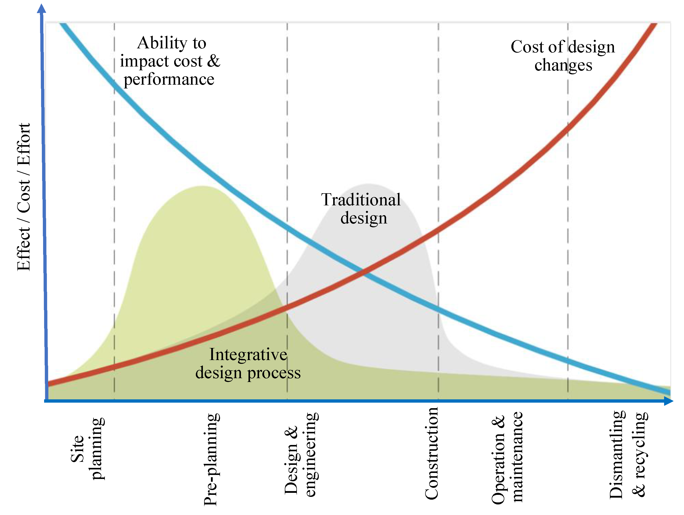
5. Optimizing the Design of the PV Solar Power Plant

The PV solar power system design is optimized to increase performance and reduce operating costs. The MacLeamy curve shown in Figure 18 shows that the sooner changes are made, the better and the cheaper the whole process is. The developer can optimize their PV solar power system at the very early stage of the project by adjusting the pitch distance and AC/DC ratio and accelerating PV by speeding up the time to layout and reducing the levelized cost of energy (LCOE). Thus, the efficiency is improved and more generation is obtained from the PV solar system. There are immediate improvements and some of the following solutions are implemented:

• Site evaluation factors, such as solar resources, the geometry of the site, the interconnection strategy, grid requirements, local restrictions, market situations, row orientation, and the shade stripe [92,93].
• The optimization of cleaning solutions, which is paramount to lowering the cost and increasing the performance and profitability of the plants [55]. The cleaning solutions can be classified as manual, semiautomated, and automated. Manual cleaning is typically done in regions in which labor is cheap. Tractors and brushes in areas with low soiling rates require low cleaning frequencies. Semiautonomous robots are cheap and typically used for smaller projects with high amounts of soiling and labor. Fully autonomous robots are typically used for remote projects in regions with extreme weather and soiling conditions that require a high cleaning frequency [52]. Each solution has different concerns, needs, and water availabilities. Soiling management solutions have lower costs per MW, increasing the site’s profitability [53].
• Configuration parameters, such as [94]

  -

  The preliminary design and equipment selection.

  -

  A PV solar system’s bill of materials (BoM) includes the PV modules’ encapsulates, front surface, back sheet, and interconnections, as well as inverters (central/ string) and module mounting systems, such as horizontal single-axis trackers, and a fixed tilt.

  -

  The optimal ground coverage ratio (GCR) is around 3–3.5. A higher GCR reduces shading losses (by measuring a structure’s length and the PV’s pitch. The pitch is related to shade control. If more land is used, more land is leased, and there are longer cables, roads, or trenches and more giant perimeter fences or greater vegetation management).

  -

  The DC/AC ratio (the ratio between the DC capacity of the array compared to the AC capacity of the inverters). The optimal value is around 1.17.

  -

  The clipping loss (this phenomenon happens when the array’s maximum power point tracking (MPPT) is greater than the maximal power available from the inverter). A high ratio can provoke a clipping loss. The inverter cannot work under these conditions.

  -

  Economic aspects of the inverter, including the cost, electrical balance of the system’s costs (BoS) (the BoS encompasses all components of a PV solar system, other than the PV system’s panels. It includes the wiring, switches, amounting systems, solar inverters, battery banks, and chargers).

  -

  The aging of the equipment.

• The final equipment selection.

  -

  The final optimization of the selected component and the final layout drawings.

  -

  The layout research algorithm presents the preliminary equipment and helps to explore possible configurations to minimize the LOCE.

  -

  A suitable components rating should be installed based on how much PV solar power plant is generated.

  -

  The PV solar system structure’s (bifacial/monofacial) arrays, the (string/central) inverters, and the (tracker/ fixed) arrays depend on the topography analogies of the site and the amount of power [95].

  -

  Weather station selection such as dust detection sensor should meet the PV solar power plant location.

  -

  Monitoring systems abroad [96].

• Operation and maintenance [97]:

  -

  The owner employs the entire in-house maintenance staff and provides all operations and maintenance tasks.

  -

  Full-turn key operational and maintenance contracts that give ability and performance guarantees to the power plant owners.

  -

  Capex investment and secure life value of up to 20–30 years of maintenance. Capex is calculated based on the infrastructure equipment and installation [98].

• Performance enhancement using intelligent solutions:

  -

  The power purchase agreement (PPA) is a contractual agreement between energy sellers and buyers.. A PPA is usually signed for a long-term period of 10–20 years.

  -

  The industry always strives for innovations, long-term views, the implementation of new technologies, and the ability to monitor performance.

  -

  The LCOE is beneficial as it compares systems built with different technologies by giving the currency value per unit of energy. There is a simple balance between an efficient project in terms of energy production and an economically viable one that reduces capital investment and operational costs.

  -

  There should be no escalation of operating expenses (OpEx) (the day-to-day expenses that a company has to keep its business running.). Thus, a flat OpEx means that whatever is paid on day one is the same as that paid in year 20.

6. System Under Study

Recently, PV systems have increasingly been integrated with the electrical grid in Jordan, facilitating procedures. One of the most important grid-connected PV systems is Quweira solar power plant, a 103 MW photovoltaic power station owned by the Quweira/Aqaba government, as shown in Figure 19 (It is located in the south of Jordan (29.76 N; 35.37 E)). The Enviromena power system is the contractor. Construction began in 2016, with a commission date of 26 April 2018. The annual net output is around 227 GWh. The Jordanian government is the owner, and The National Electrical Power Company (NEPCO) is the operator. The construction cost was around ($120 million). The nameplate capacity of the 103 MW-DC is divided into two areas: a fixed plant of 52.610 MW-DC and a tracked plant of 52.578 MW-DC. The irradiance and temperature values are obtained hourly from the SCADA system. The Quweira PV Plant project includes eight strings of MV-connected PV inverter stations. Every two strings are connected in a loop/ring. Thus, the continuity of supply is maintained by having a total of 4 ring connections. They are connected to the 2 × 33/132 kV transformers. The arrays used are the Jinko Solar JKM 315pp. The PV plant has 38 inverter transformers with a rating of 3150 kVA and a step-up ratio of 33/0.4 kV. These inverters are the Ingecon Sun Power Max 500TL X400—1050 kVA. The inverter transformers are connected via single-core XLPE cables with a cross-sectional area of 240 mm${}^2$ or 300 mm${}^2$ via 8 string connections to the 33 kV side of the Quweira substation. The station generated 214,636 MWh in the first year, and its performance ratios were $79.8\%$ and $79.2\%$ for the fixed and tracked plants, respectively. The total module quantity is 328,320 modules. There are 164,160 PV modules with a fixed-tilt PV installation and 164,160 PV modules with a tracker PV installation.

Typically, fixed solar panel arrays are mounted on a sloping roof with a carefully selected orientation, e.g., facing straight south in the northern hemisphere. The two ways that the sun traverses the sky are horizontally, as it moves from east to west, and vertically, as it rises and falls. The angle of incidence at which the sun’s rays strike the panel’s surface changes and becomes more oblique as it passes across its face. As a result, the ability of the solar cell crystals to convert energy is diminished. Trackers that only follow one axis—horizontal movement—are known as single-axis trackers, and dual-axis trackers follow both axes. Single-axis trackers can recover up to $45\%$ more of the sun’s energy, while dual-axis models can save a massive $65\%$, so they work well. Unfortunately, they are costly and inappropriate for all circumstances, but they are still worth considering.

A central converter outfitted with three or four blocks connected to the same PV and a medium voltage transformer in parallel.

Table 7. Quweria PV power plant’s rating capacity.

Total capacity	105.19 MW DC
Fixed plant capacity	52.61 MW DC
Tracked plant capacity	52.61 MW DC
Support structure	$50\%$ Fixed + $50\%$ Tracked
Nominal PV power	103,000 kWp
Nominal AC power	81,935 kWAC
Pnom ratio	1.257
Total PV plant generation (MWh)	214,636
Capacity factor of both parts of the plant	0.233
The PV plant’s self-consumption (MWH)	1237
Self-consumption to generation $(\%)$	$0.58\%$

shows the Quweira PV power plant’s rating capacity.

Table 8. Quweira PV power plant’s main components.

Modules	JinkoSolar JKM315PP-72
Inverters	Ingeteam IS 1000TL X400
Modules in series	20
No. of strings	8640
No. of modules	172,800
Module area	335,293 m${}^2$

shows the plant’s main components.

Table 9. Quweira PV power plant module’s mechanical characteristics.

Cell type	Polycrystalline $156\times 156$ mm (6 inch)
N${}^{\circ }$ cell	72 $(6\times 12)$
Dimensions (mm)	$1956\times 992\times 40$
Weight (kg)	26.5 kg (58.4 Ibs)
Front glass	4 mm transmission, low iron, tempered glass

shows the mechanical characteristics of the Quweira PV power plant module.

Table 10. Quweira PV power plant’s array specifications.

Specifications	JKM315P(STC)
Maximum power (Pmax)	315 Wp
Maximum power voltage (Vmp)	37.2 V
Maximum power current (Imp)	8.48 A
Open circuit voltage (Voc)	46.2 V
Short circuit current (Isc)	9.01 A
Module efficiency under STC $(\%)$	16.23 $(\%)$
Operating temperature (${}^{\circ }$C)	∼40 ${}^{\circ }$C ∼+85 ${}^{\circ }$C
Maximum system voltage	1000 VDC (ETL)
Maximum series fuse rating	15 A
Power tolerance	0∼+3%
Temperature coefficients of Pmax	$-0.04\%{/}^{\circ }$C
Temperature coefficients of Voc	$-0.03\%{/}^{\circ }$C
Temperature coefficients of Isc	$0.05\%{/}^{\circ }$C
Nominal operating cell temperature (NOCT)	$45\pm 2{}^{\circ }$C

shows the Quweira PV power plant’s array specifications.

Table 11. Quweira PV power plant’s central inverter specifications.

Type	INGECON-SUN-1000 TL U X400 Outdoor
Recommended PV array power range	892.6–1178.3 kWp
Voltage range MPP	581–820 V
Maximum voltage	1000 V
Maximum current	1800 A
$N^o$ of inputs with fuse holders	8–16 (16–32 for floating configuration)
Type	connection to copper bars
Frequency	50/60 Hz
Phi Cosine	1
Phi Cosine adjustable	Yes, Smax = 1220 kVA
THD (total harmonic distortion)	$\prec 3\%$
Maximum efficiency	$98.6\%$
Standby consumption	120 W
Consumption at night	120 W

shows the Quweira PV power plant’s central inverter specifications.

Table 12. Quweira PV power plant’s cable and transformer specifications.

Cable	$1\times (3\times 1\times 300)$ mm${}^2$ $\mathrm{XLPE}18/30\left(36\right)\mathrm{kV}\mathrm{AL}$
Transformer	315 kVA-oil typeDYN11YN11YN11 33 kV/0.4 kV/ 0.4 kV/0.4 kV ONAN

shopws the Quweira PV power plant’s cable and transformer specifications.

7. Results and Discussion

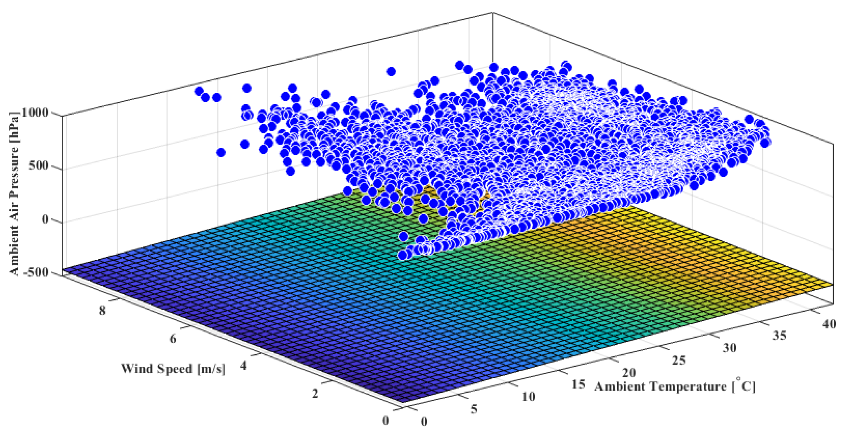
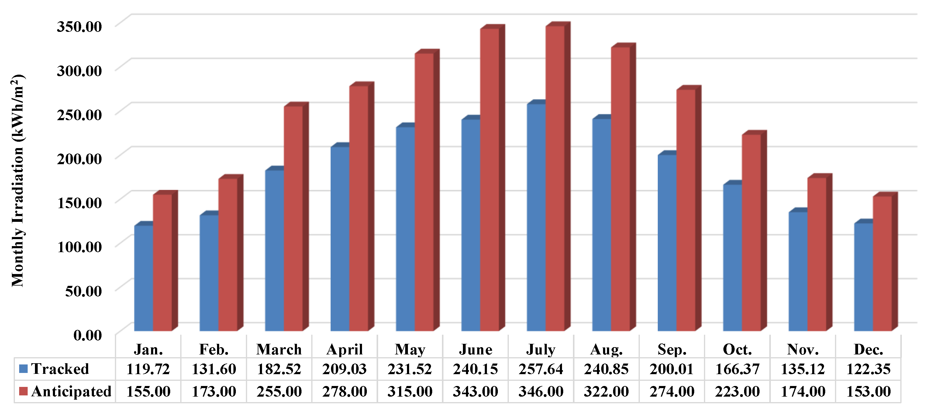
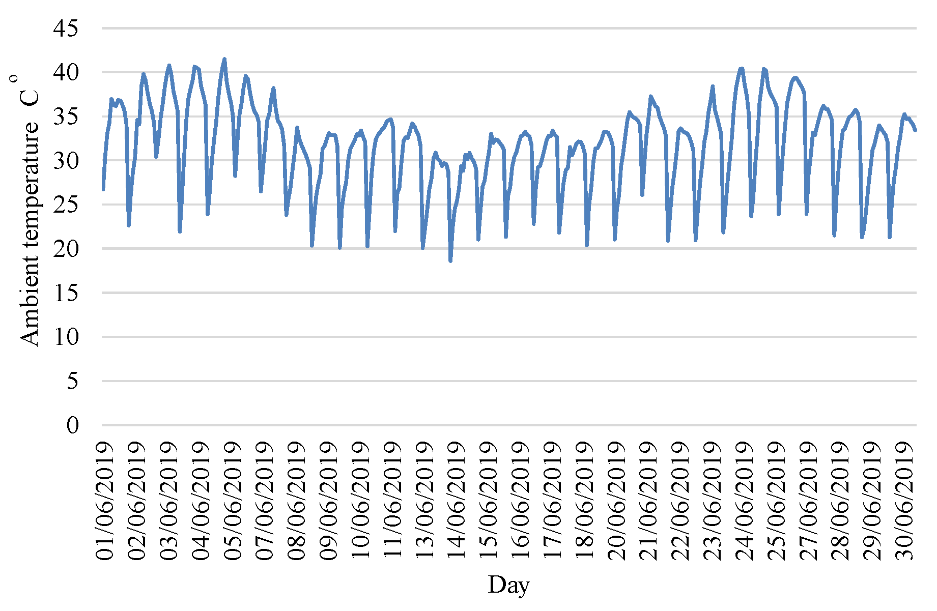
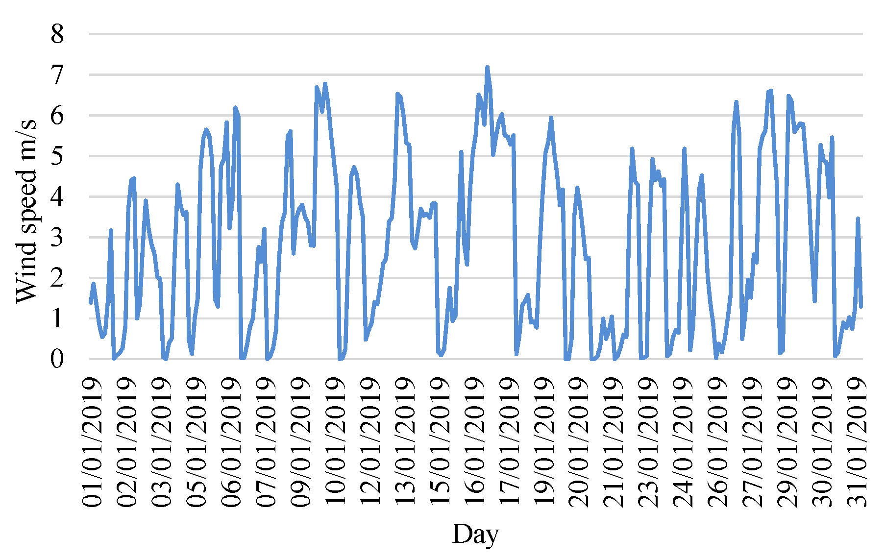
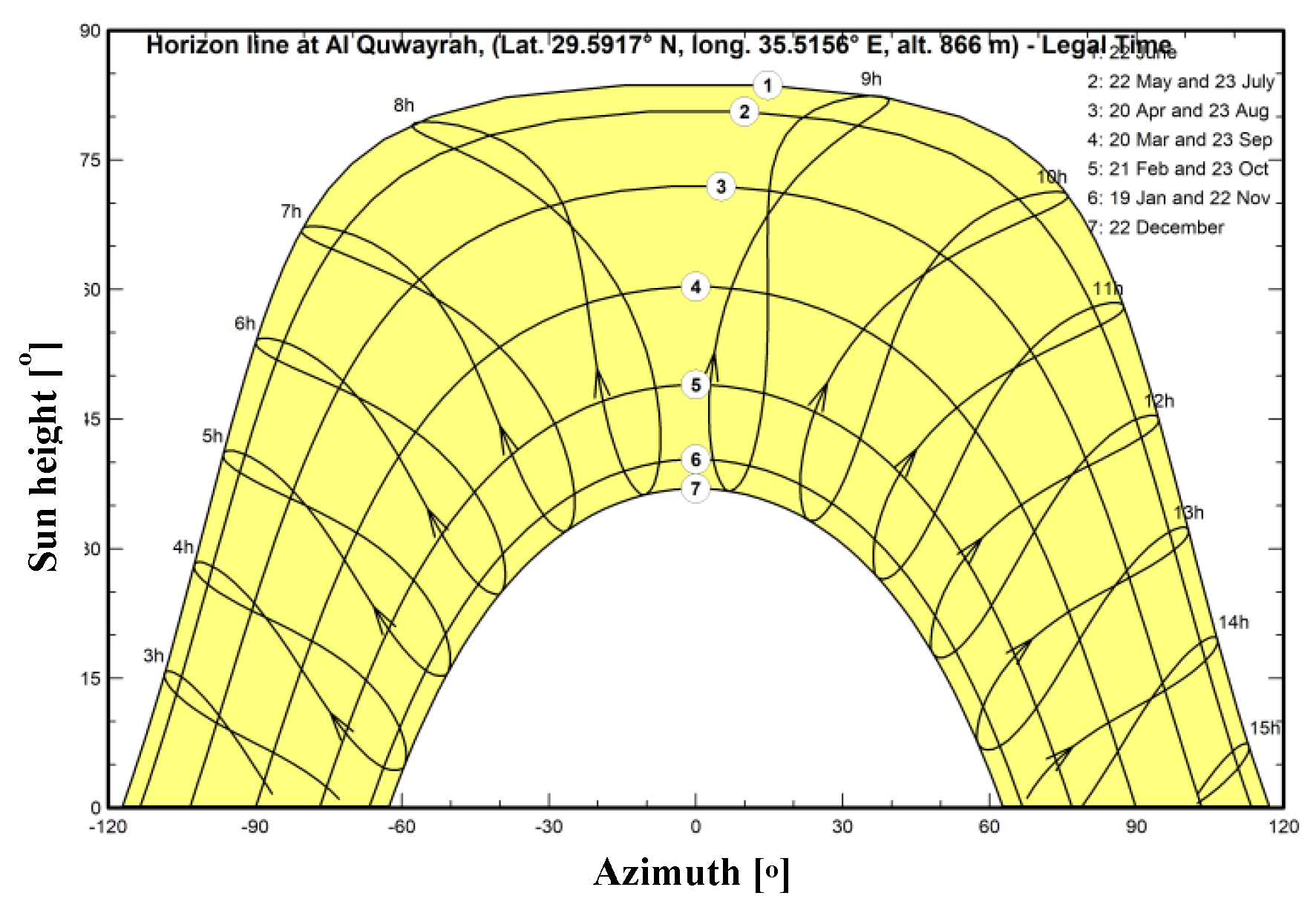
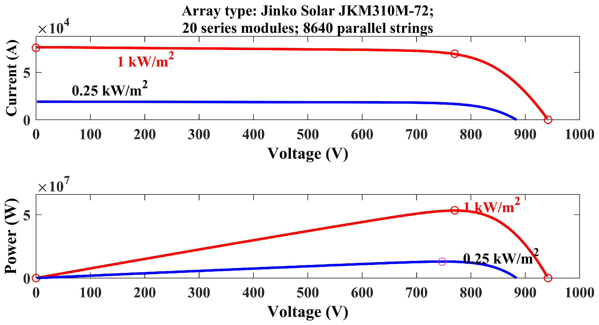
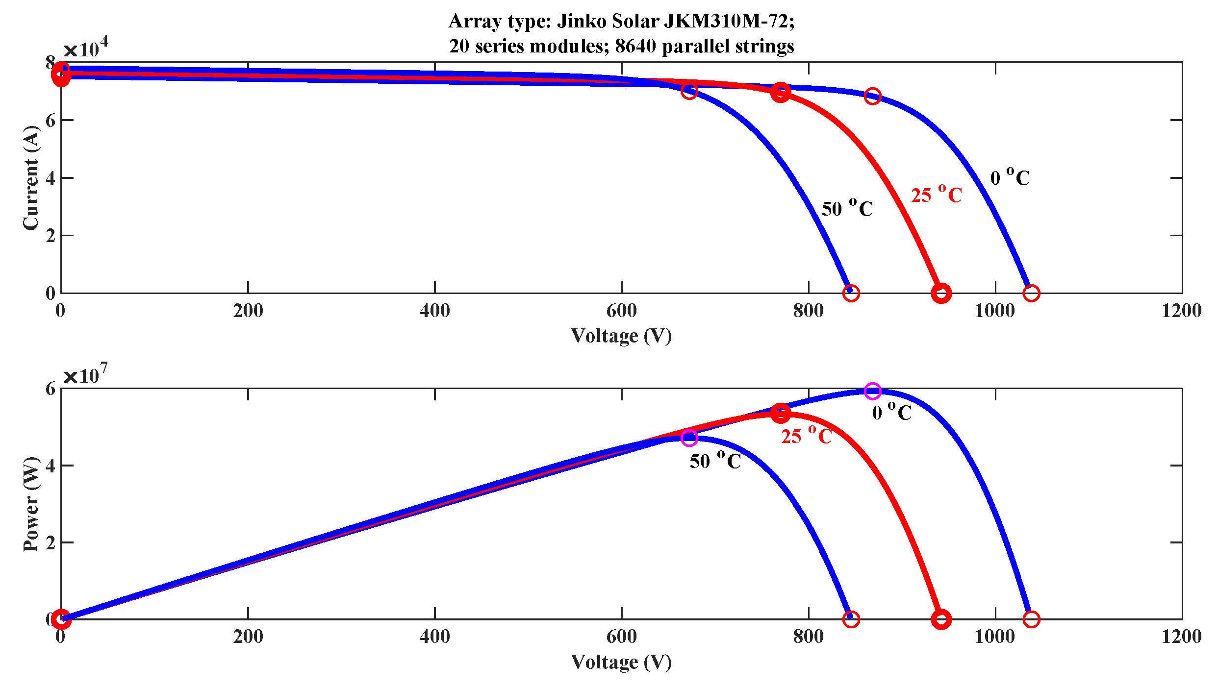
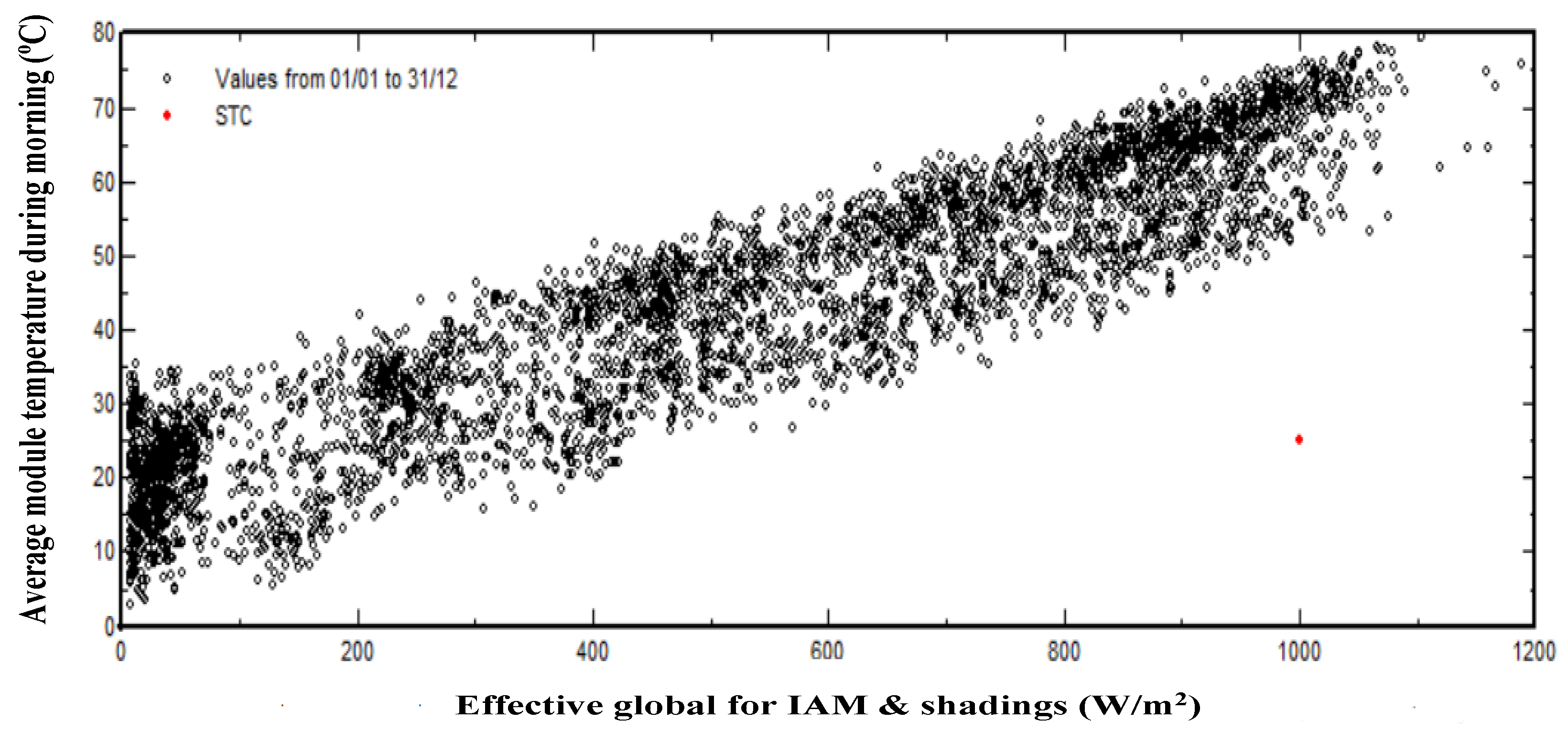
Figure 20 shows the wind speed as a function of the ambient temperature and pressure at the Quweria PV power plant. Figure 21 shows the typical vs. the measured values of POA Irradiance for the fixed plant. Figure 22 shows the typical vs. the measured values of POA irradiance for the tracked part plant. Figure 23 shows a sample of ambient temperatures (${}^{\circ }$C) at the location of the system under study. Figure 24 shows a sample of wind speeds. Figure 25 shows sun paths (height/Azimuth diagram). The total PV arrays are represented by 20 modules connected in series and 8640 strings connected in parallel. Figure 26 demonstrates the characteristics of the PV array at different irradiation levels for the combined arrays used. Figure 27 demonstrates the characteristics of the combined PV array at different temperatures. Figure 28 shows the array temperature vs. the effective irradiance.

As mentioned in this work, PV power plant losses include thermal losses. The thermal balance in the PVsyst software involves the heat loss factor, known as U. It is calculated as shown in Equation (22)

$$U=U_c+U_v+win{d}_{vel}$$

(22)

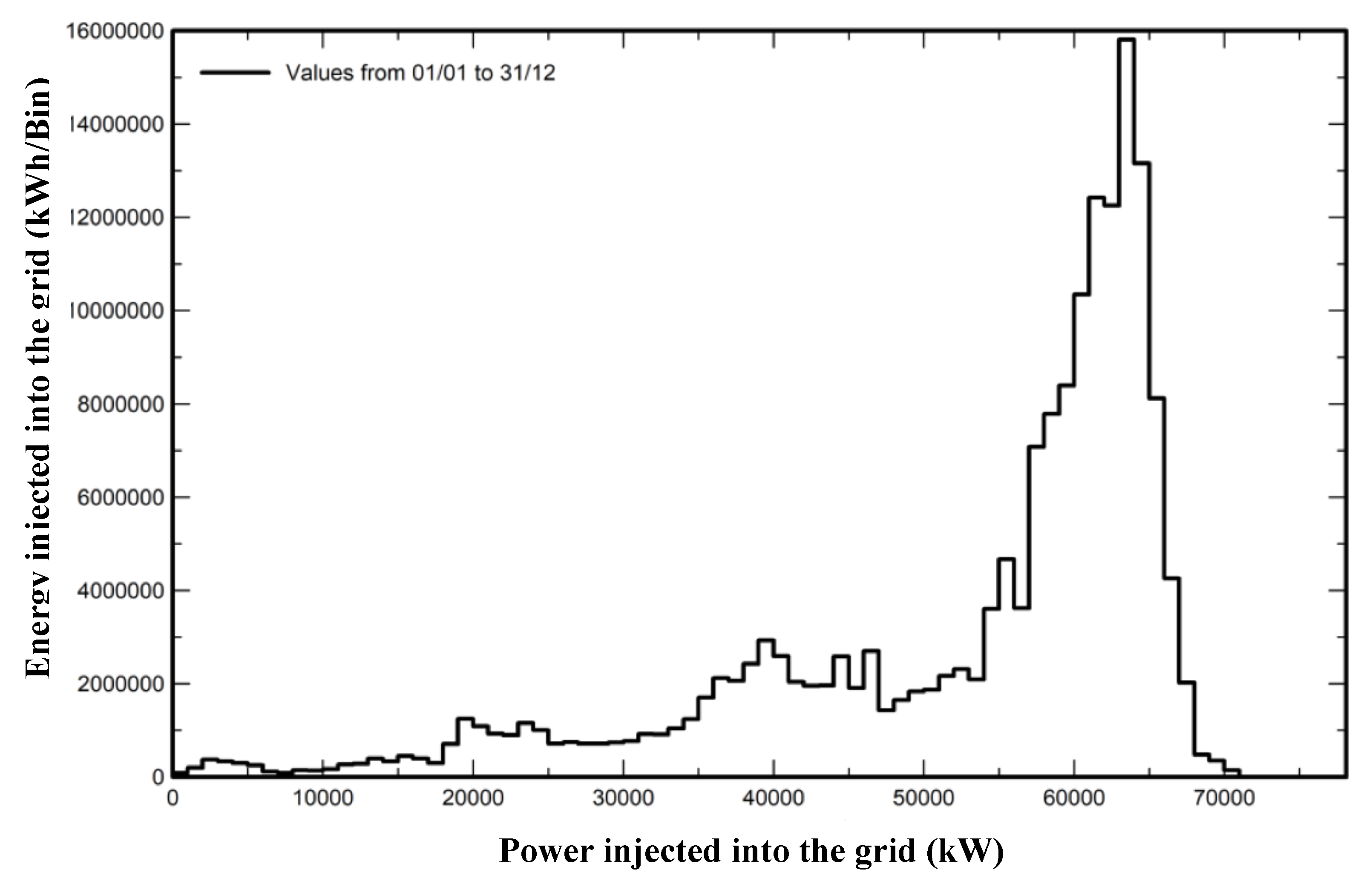
where $U_c$ is the constant loss factor, W/m${}^2$ K, $U_v$ is the wind loss factor (W/m${}^2$ K m/s), and $win{d}_{vel}$ is the wind velocity (m/s).

Table 13. Balances and main results.

Months	GlobHor (kWh/m2)	DiffHor (kWh/m2)	TAmb (°C)	GlobInc (kWh/m2)	GlobEff (kWh/m2)	EArray (GWh)	EGrid (GWh)	PR Ratio	EArrMPP (GWh)	EArray (GWh)
January	109.1	31.00	9.70	157.0	149.6	12.63	12.16	0.748	13.56	12.63
February	120.4	34.72	10.93	160.1	152.1	12.81	12.34	0.748	13.69	12.81
March	165.5	48.05	14.55	198.3	188.9	15.45	14.87	0.728	16.63	15.45
April	193.2	53.7	19.7	210.5	200.4	15.94	15.35	0.708	17.17	15.94
May	225.1	58.59	23.63	228.9	217.3	17.06	16.41	0.696	18.22	17.06
June	236.4	54.00	25.56	238.5	226.8	17.59	16.93	0.689	18.79	17.59
July	236.8	55.49	27.00	240.5	229.0	17.77	17.09	0.690	18.88	17.77
August	219.8	51.46	27.18	238.3	227.2	17.53	16.87	0.687	18.70	17.53
September	180.3	45.3	25.73	208.7	198.6	15.32	14.73	0.686	16.43	15.32
October	145.1	40.61	21.97	185.6	176.1	14.26	13.72	0.718	15.08	14.26
November	112.2	31.5	16.45	159.6	151.5	12.59	12.1	0.736	13.32	12.59
December	98.6	29.45	11.35	149.8	142.1	12.32	11.86	0.768	12.9	12.32
Year	2042.5	533.87	19.52	2376.3	2259.4	181.28	174.42	0.713	193.36	181.28

shows the balances and main results, where GlobHor is the global horizon irradiation, DiffHor is the horizontal diffuse irradiation, $T_{Amb}$ is the ambient temperature, GlobInc is the global incident in the collector plane, GlobEff is the effective global correlation for the IAM and shading, EArray is the effective energy at the output of the array, $E_{Grid}$ is the energy injected into the grid, PR is the performance ratio, EArrMPP is the array’s virtual energy at the MPP, and EArray is the effective energy at the output of the array.

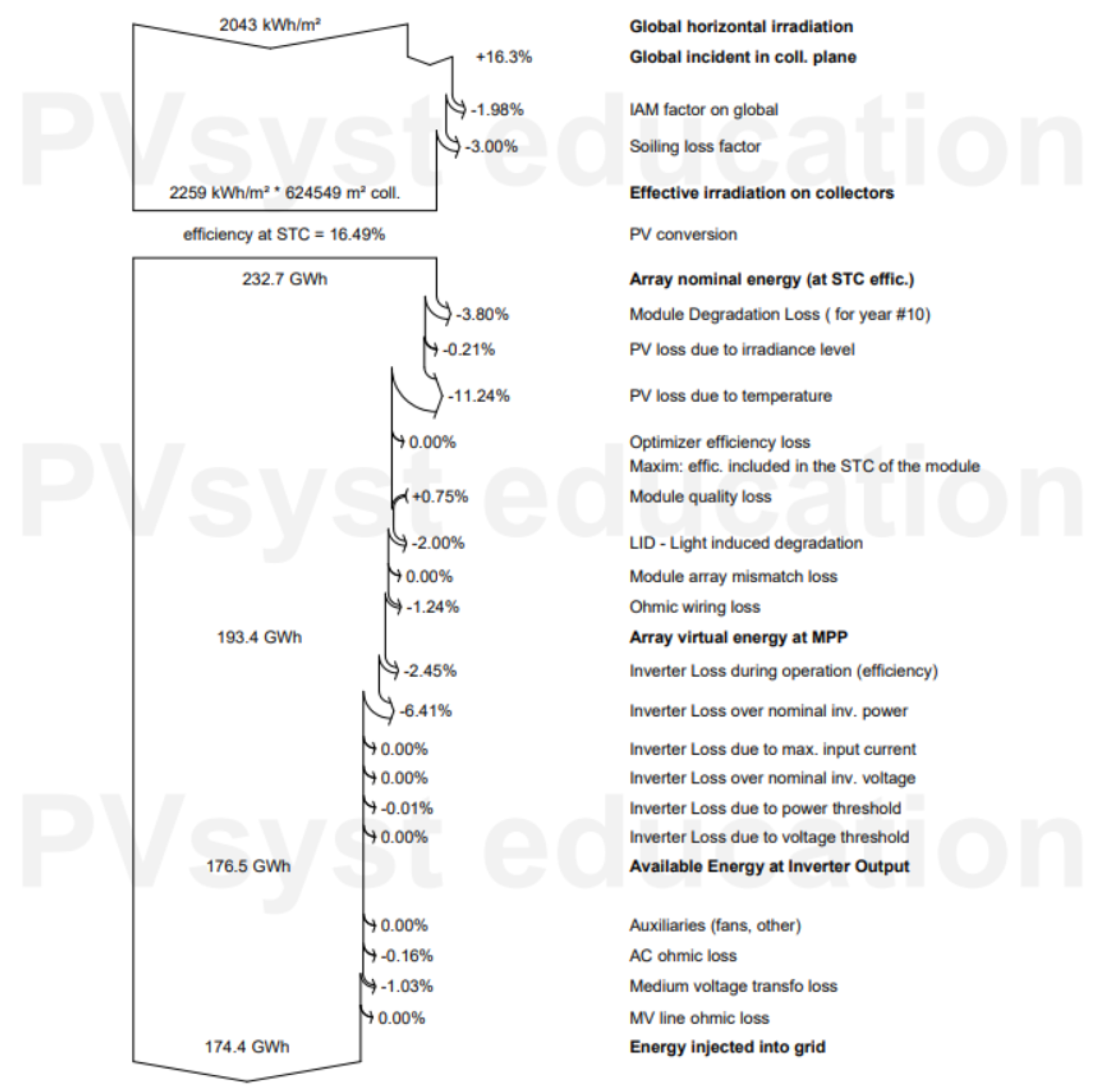
The main parameter needed for the wiring losses of the PV array is the resistance of the circuit according to the wire lengths and sections. Wiring loss may be evaluated as a percentage of the system’s power under STC. Losses of cables between the output of the inverter and the injection point of the energy meter should be considered. The distance and wire section should be defined earlier. The external transformer loss should be considered in a high rating system (MW). The LID mismatch parameter reflects the confidence of matching the actual module set’s performance concerning the manufacturer’s specifications. The default PVsyst value is half of the lower tolerance level for the module’s exposure to the sun. A typical value for the LID loss factor for P-type wafers is $2\%$. The current mismatch within a string is essential, because the current in the weakest module dominates the current in the whole string.Voltage mismatch between strings has a lower impact on the system’s performance. The soiling loss is almost negligible in temperate climates and residential situations. It may become very significant in some industrial environments, such as systems near railway lines or in a desert climate. Each month, the soiling loss can be defined individually to account for periodic cleaning, rainy periods, or eventual snow covering. The soiling loss factor is $3\%$. IAM is defined in the PV module within the component database. Specific studies can be conducted using a standard profile based on Fresnel’s laws. The auxiliaries include fans, air conditioners, and electronic devices. Thus, Figure 29 shows the loss flow diagram for the plant under study. Figure 30 shows the plant’s power output distribution. Figure 31 shows the normalized production per installed kWp.

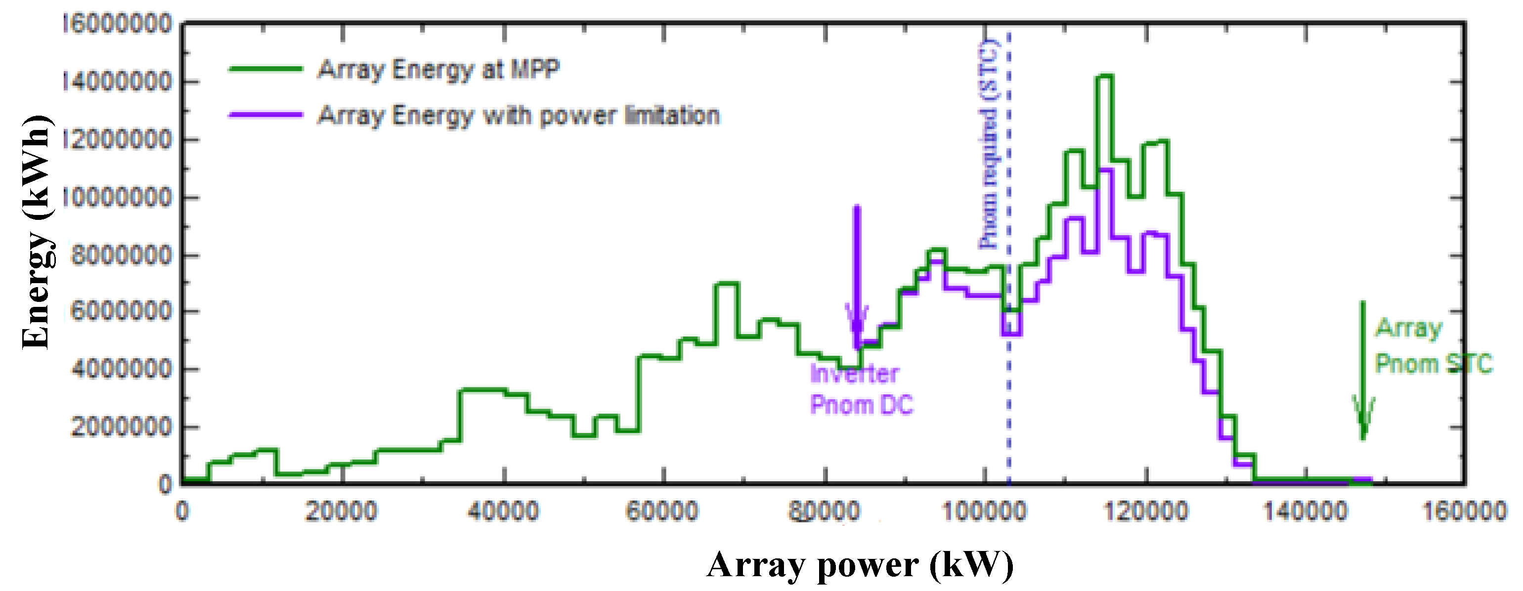
Figure 32 shows the nominal power at the input of the inverter. The operating conditions above these values are limited. The violet curve shows the power, and the green curve shows the power available from the array. In case the array is working at its MPP. The difference between these two curves represents the overload power loss. The overload power loss percentage is the area between these curves concerning the entire histogram area. PVsyst software considers the sizing to be acceptable when the overload loss does not exceed $3\%$. When the overload loss is 1–3%, PVsyst software shows a slightly undersized inverter and has an orange warning. However, if the overload exceeds $3\%$, PVsyst software gives an error message in red, and the simulation is impossible. If the designer wants to create a system with a highly oversized PV array, they need to increase the potential limit of $3\%$ in the project’s settings. The nominal power $P_{nom-ratio}$ is known as the DC/AC ratio. A good sizing usually corresponds to a $P_{nom-ratio}$ of 1.25–1.3. Note that the simulation’s overload loss may significantly differ from the sizing value. The histogram calculation for this rough sizing tool cannot consider all system losses. Thus, the ratio of the inverter loss to the nominal inverter power is $-1.89\%$.

One of the most critical electrical specifications in the PV solar system is the panel efficiency [100,101]: the higher the efficiency, the smaller the surface area needed to generate a specific output power. The size of the PV array is based on the energy production in the darkest time of the year. Additionally, the panel output depends on the insulation, temperature, and $R_L$. The inverter size should match the array size. Additionally, the inverter size is based on the $R_L$ peak. The PV’s output voltage must be within the appropriate range in all weather conditions throughout the year. The inverter’s efficiency varies depending on the $R_L$. Simultaneously, extra cooling might be needed when the temperature is over ${40}^{\circ }$. Thus, system design begins by analyzing the loads that need to be powered.

PR (performance ratio) is an essential tool or factor that is used globally by companies and professionals to assess the healthiness of solar PV plants [102,103]. It is considered an important metric in the PV industry. When commissioning a PV system, it is often used as a contractual condition and part of the warranty. It is not altered by the system’s size or type. It is the ratio of the effective produced energy to the ideal energy yield under STC. Usually, the energy produced is the available usable energy delivered to the end-user or the grid. The PR ratio includes the optical, PV array, DC to AC conversion, and other plant losses. A simple annual PR is measured based on actual the usable energy and the annual solar irradiance [104]. It is considered an indication of the peak capacity of the PV power plant and is independent of the location-specific irradiance [105]. It is given by Equation (23)

$$PR=\frac{E\times G_{STC}}{P_p\times G_{POA}}\times 100\%$$

(23)

where E is the electricity generation (kWh/year), $P_p$ is the PV module’s installed capacity (kWp), $G_{POA}$ is the total global solar irradiation sum on the plane of the array (kWh/m${}^2$/year), and $G_{STC}$ is the global solar irradiance under STC = 1 kW/m${}^2$. PR can be classified into two types based on its significance and applicability. First, there is the STC equivalent PR. This is calculated by adjusting the power at each recording interval to compensate for the difference between the actual PV module temperature $T_{ambient}$ and the STC reference temperature at $25{}^{\circ }$C. This method is normally used when the plant’s PR is to be measured for a short duration in the day. Second, there is the annual temperature corrected PR. This calculates the PR during the reporting period using the power at each recording interval to compensate for the difference between the actual PV module’s temperature $T_{ambient}$ and the expected annual average module’s temperature. The annual temperature correction is significant when the annual PR must be validated within the first 15–20 days of operation.

Table 14. Monthly PR (2021) [99].

Month	January	February	March	April	May	June	July	August	September	October	November	December
PR %	85.3	84.1	82.3	80.5	78.7	77.4	77.1	77.2	78.6	81.2	83.4	85.1

shows the monthly PR [99]. It shows that the plant is healthy and verifies the annual energy yield [106,107].

Table 15. Main outputs for the plant under study.

System’s production	174,419 MWh/year
Specific production	1693 kWh/kWp/year
Performance ratio	$80.9\%$
Normalized production	4.64 kWh/kWp/day
Array losses	1.69 kWh/kWp/day
System losses	0.18 kWh/kWp/day

shows the main output for the plant under study [108].

Optimizing a PV plant’s design increases its performance and reduces the operating costs. The PV solar system development process can be classified into fixed design development processes, including a regulatory framework, project site specifications, solar resources, and client requirements. The configuration analysis includes equipment selection, the design of the plant’s layout, contracting, and operational strategies—the iterative processes concerns energy efficiency and yield calculations. Usually, grid outages and equipment shutdowns are not considered as part of the PV solar system’s efficiency, despite representing 2–3% of the total energy loss. Most losses are associated with the components’ characteristics and design issues. Some approaches can help to reduce these losses, such as regular maintenance, shading prevention, and regular cleaning to guarantee that the maximal amount of sun energy reaches the panel’s surfaces. The equipment for the system under study, such as the panels, mounting structures, combiner boxes, warehouses, sensors, and especially, the pyranometers, appeared to be clean and in good operating condition; even the internal roads were clean. The site security is controlled and monitored by gates and fences and was found to be in acceptable shape. The scheduled preventive and corrective maintenance activities are performed regularly. A random spot check of the PV module was executed. It is worth mentioning that the Quwiera PV power plant is an optimal case, corresponding to a DC/AC ratio of 1.17, a GCR of 3.1, and a PR of $80.9\%$.

8. Conclusions

An adequate PV solar system has a high level of performance, long-term efficiency, and durability. Thus, putting effort into PV solar system losses can potentially exceed financial savings. The next step is to match the power use by shifting the load to the free electricity generation period. Understanding the PV solar loss asset management strategies can boost solar performance. Hence, the industry should develop technologies in succession and plan to prevent and reduce these losses. This review discussed the various causes of PV system losses. There have been many developments to minimize these losses in PV, such as improving the quality of materials using bifacial solar panels that use front and rear irradiation. System components have losses in energy between states, a decreased range, an increased weight/volume, and the creation of heat. Characterizing losses can help us to understand, mitigate, and manage them using the most accurate measurements to achieve reasonable measures for the derived values. Reducing a PV solar system’s losses maximizes its power output and return. This work presented a study of grid-tied PV solar systems using PVsyst software. The analysis showed that the PR of the system under study is $80.9\%$. The measured yields for the fixed and tracked systems were 98,800 MWh and 115.835 MWh, respectively. Future work will discuss the optimization of PV solar power plant design to improve performance and reduce operating costs.

References

- Humada, A.M.; Hojabri, M.; Mekhilef, S.; Hamada, H.M. Solar cell parameters extraction based on single and double-diode models: A review. Renew. Sustain. Energy Rev. 2016, 56, 494–509. [Google Scholar] [CrossRef]
- Ong, N.A.F.M.N.; Sadiq, M.A.; Said, M.S.M.; Jomaas, G.; Tohir, M.Z.M.; Kristensen, J.S. Fault tree analysis of fires on rooftops with photovoltaic systems. J. Build. Eng. 2022, 46, 103752. [Google Scholar]
- Köntges, M.; Kurtz, S.; Packard, C.; Jahn, U.; Berger, K.A.; Kato, K.; Friesen, T.; Liu, H.; Van Iseghem, M.; Wohlgemuth, J.; et al. Review of Failures of Photovoltaic Modules; Kontges, M., Kurtz, S., Packard, C., Jahn, U., Berger, K.A., Kato, K., Friesen, T., Liu, H., Van Iseghem, M., Eds.; Report IEA-PVPS T13-01; International Energy Agency: Paris, France, 2014; pp. 33–35. [Google Scholar]
- Micheli, L.; Ruth, D.; Muller, M. Seasonal trends of soiling on photovoltaic systems. In Proceedings of the 2017 IEEE 44th Photovoltaic Specialist Conference (PVSC), Washington, DC, USA, 25–30 June 2017; pp. 2301–2306. [Google Scholar]
- Mithhu, M.M.H.; Rima, T.A.; Khan, M.R. Global analysis of optimal cleaning cycle and profit of soiling affected solar panels. Appl. Energy 2021, 285, 116436. [Google Scholar] [CrossRef]
- Rouani, L.; Harkat, M.F.; Kouadri, A.; Mekhilef, S. Shading fault detection in a grid-connected PV system using vertices principal component analysis. Renew. Energy 2021, 164, 1527–1539. [Google Scholar] [CrossRef]
- Santos, A.V.; Canavarro, D.; Collares-Pereira, M. The gap angle as a design criterion to determine the position of linear Fresnel primary mirrors. Renew. Energy 2021, 163, 1397–1407. [Google Scholar] [CrossRef]
- Sporleder, K.; Turek, M.; Schüler, N.; Naumann, V.; Hevisov, D.; Pöblau, C.; Großer, S.; Schulte-Huxel, H.; Bauer, J.; Hagendorf, C. Quick test for reversible and irreversible PID of bifacial PERC solar cells. Sol. Energy Mater. Sol. Cells 2021, 219, 110755. [Google Scholar] [CrossRef]
- Nguyen, D.C.; Ishikawa, Y.; Jonai, S.; Nakamura, K.; Masuda, A.; Uraoka, Y. Elucidating the mechanism of potential induced degradation delay effect by ultraviolet light irradiation for p-type crystalline silicon solar cells. Sol. Energy 2020, 199, 55–62. [Google Scholar] [CrossRef]
- Lim, J.; Kim, M.; Park, H.H.; Jung, H.; Lim, S.; Hao, X.; Choi, E.; Park, S.; Lee, M.; Liu, Z.; et al. Kinetics of light-induced degradation in semi-transparent perovskite solar cells. Sol. Energy Mater. Sol. Cells 2021, 219, 110776. [Google Scholar] [CrossRef]
- Tian, Y.; Liu, X.; Ghanekar, A.; Zheng, Y. Scalable-manufactured metal–insulator–metal based selective solar absorbers with excellent high-temperature insensitivity. Appl. Energy 2021, 281, 116055. [Google Scholar] [CrossRef]
- Goswami, A.; Sadhu, P.K. Degradation analysis and the impacts on feasibility study of floating solar photovoltaic systems. Sustain. Energy Grids Netw. 2021, 26, 100425. [Google Scholar] [CrossRef]
- Winston, D.P.; Karthikeyan, G.; Pravin, M.; JebaSingh, O.; Akash, A.; Nithish, S.; Kabilan, S. Parallel power extraction technique for maximizing the output of solar PV array. Sol. Energy 2021, 213, 102–117. [Google Scholar] [CrossRef]
- Sarquis Filho, E.A.; Fernandes, C.A.F.; da Costa Branco, P.J. A complete framework for the simulation of photovoltaic arrays under mismatch conditions. Sol. Energy 2021, 213, 13–26. [Google Scholar] [CrossRef]
- Ahmed, D.R.; Mohammed, I.R.; Abdullah, H.M.; Muhammadsharif, F.F.; Sulaiman, K.; Alsoufi, M.S.; Bawazeer, T.M. The Correlation of Device Parameters with Illumination Energy to Explore the Performance of a Monocrystalline Silicon Solar Module. Silicon 2021, 14, 1439–1445. [Google Scholar] [CrossRef]
- Zhong, X.; Ekanayake, C.; Ma, H.; Saha, T.K. Ageing Analysis of Solar Farm Inverter Transformers. IEEE Trans. Power Deliv. 2021, 36, 3815–3824. [Google Scholar] [CrossRef]
- de Barros, R.C.; da Silveira Brito, E.M.; do Couto Boaventura, W.; Pereira, H.A.; Cupertino, A.F. Methodology for bondwire lifetime evaluation of multifunctional PV inverter during harmonic current compensation. Int. J. Electr. Power Energy Syst. 2021, 128, 106711. [Google Scholar] [CrossRef]
- Tan, Z.H.; Chua, K.H.; Lim, Y.S.; Morris, S.; Wang, L.; Tang, J.H. Optimal operations of transformers in railway systems with different transformer operation modes and different headway intervals. Int. J. Electr. Power Energy Syst. 2021, 127, 106631. [Google Scholar] [CrossRef]
- Hashemi, B.; Taheri, S.; Cretu, A.M.; Pouresmaeil, E. Systematic photovoltaic system power losses calculation and modeling using computational intelligence techniques. Appl. Energy 2021, 284, 116396. [Google Scholar] [CrossRef]
- Andreani, L.C.; Bozzola, A.; Kowalczewski, P.; Liscidini, M.; Redorici, L. Silicon solar cells: Toward the efficiency limits. Adv. Phys. X 2019, 4, 1548305. [Google Scholar] [CrossRef]
- Vaqueiro-Contreras, M.; Markevich, V.P.; Coutinho, J.; Santos, P.; Crowe, I.F.; Halsall, M.P.; Hawkins, I.; Lastovskii, S.B.; Murin, L.I.; Peaker, A.R. Identification of the mechanism responsible for the boron oxygen light induced degradation in silicon photovoltaic cells. J. Appl. Phys. 2019, 125, 185704. [Google Scholar] [CrossRef]
- Baltus, C.; Eikelboom, J.; Van Zolingen, R. Analytical Monitoring of Losses in PV Systems; Energy Research Foundation: Petten, The Netherlands, 1997. [Google Scholar]
- Das, D.; Kalita, P.; Roy, O. Flat plate hybrid photovoltaic-thermal (PV/T) system: A review on design and development. Renew. Sustain. Energy Rev. 2018, 84, 111–130. [Google Scholar] [CrossRef]
- PV Magazine. 34% Year-on-Year Growth Projected in Annual PV Installations. Available online: www.pv-magazine.com/ (accessed on 20 September 2021).
- Powerweb Forecast Internationa’s Energy Portals—A Leading Provider of Power System Market Intelligence and Consulting. Available online: http://www.fi-powerweb.com/Renewable-Energy.html (accessed on 21 January 2021).
- Gajjar, J.; Agravat, S.; Harinarayana, T. Solar PV energy generation map of Karnataka, India. Smart Grid Renew. Energy 2015, 6, 333. [Google Scholar] [CrossRef]
- EEP (Energy and Environment Partnership Programme). Technical Brief—Solar PV & Energy Efficiency Phase II; National Renewable Energy Laboratory (NREL), United States Department: Golden, CO, USA, 2016. [Google Scholar]
- International Renewable Energy Agency. Renewable Capacity Statistics 2022; Technical Report; International Renewable Energy Agency: Abu Dhabi, United Arab Emirates, 2022. [Google Scholar]
- Energy & Minerals Regulatory Commission. Annual Book 2018; Energy & Minerals Regulatory Commission: Amman, Jordan, 2018. [Google Scholar]
- Roose, B.; Tennyson, E.M.; Meheretu, G.; Kassaw, A.; Tilahun, S.A.; Allen, L.; Stranks, S.D. Local manufacturing of perovskite solar cells, a game-changer for low-and lower-middle income countries? Energy Environ. Sci. 2022, 15, 3571–3582. [Google Scholar] [CrossRef]
- Brecl, K.; Bokalič, M.; Topič, M. Annual energy losses due to partial shading in PV modules with cut wafer-based Si solar cells. Renew. Energy 2021, 168, 195–203. [Google Scholar] [CrossRef]
- Villalva, M.G.; Gazoli, J.R.; Ruppert Filho, E. Comprehensive approach to modeling and simulation of photovoltaic arrays. IEEE Trans. Power Electron. 2009, 24, 1198–1208. [Google Scholar] [CrossRef]
- Sabbaghpur Arani, M.; Hejazi, M.A. The comprehensive study of electrical faults in PV arrays. J. Electr. Comput. Eng. 2016, 2016. [Google Scholar] [CrossRef]
- Bonkoungou, D.; Guingane, T.; Korsaga, E.; Tassembedo, S.; Koalaga, Z.; Darga, A.; Zougmore, F. A novel topology to improve PV module efficiency under partial shading conditions. Int. J. Photoenergy 2022, 2022. [Google Scholar] [CrossRef]
- Sukhatme, S.P. Principles of Thermal Collection and Storage; Tata McGraw-Hill Publishing Company: New York, NY, USA, 2017. [Google Scholar]
- Solemetric. Shade Measurements and PV Design, Solar Site Evaluation: Tools and Techniques to Quantify and Optimize Production. SolarPro Magazine 2018. [Google Scholar]
- Li, C. Comparative performance analysis of grid-connected PV power systems with different PV technologies in the hot summer and cold winter zone. Int. J. Photoenergy 2018, 2018, 8307563. [Google Scholar] [CrossRef]
- Appiah, A.Y.; Zhang, X.; Ayawli, B.B.K.; Kyeremeh, F. Review and performance evaluation of photovoltaic array fault detection and diagnosis techniques. Int. J. Photoenergy 2019, 2019, 6953530. [Google Scholar] [CrossRef]
- Namikawa, S.; Kinsey, G.; Heath, G.A.; Wade, A.; Sinha, P.; Komoto, K. Photovoltaics and Firefighters’ Operations: Best Practices in Selected Countries; Technical Report; National Renewable Energy Lab. (NREL): Golden, CO, USA, 2017. [Google Scholar]
- Bernadette, D.; Twizerimana, M.; Bakundukize, A.; Pierre, B.J.; Theoneste, N. Analysis of Shading Effects in Solar PV System. Int. J. Sustain. Green Energy 2021, 10, 47. [Google Scholar] [CrossRef]
- Kaddour, A.; Benmebrouk, L.; Bekkouche, S.A.; Benyoucef, B.; Bezari, S.; Khenniche, R. Improvement of the Stand-Alone PV System Performance by PVSYST Software. In Proceedings of the 2019 7th International Renewable and Sustainable Energy Conference (IRSEC), Agadir, Morocco, 27–30 November 2019; pp. 1–6. [Google Scholar]
- Boppana, S.; Passow, K.; Sorensen, J.; King, B.H.; Robinson, C. Impact of uncertainty in IAM measurement on energy predictions. In Proceedings of the 2018 IEEE 7th World Conference on Photovoltaic Energy Conversion (WCPEC) (A Joint Conference of 45th IEEE PVSC, 28th PVSEC & 34th EU PVSEC), Waikoloa, HI, USA, 10–15 June 2018; pp. 2276–2281. [Google Scholar]
- Dey, D.; Subudhi, B. Design, simulation and economic evaluation of 90 kW grid connected Photovoltaic system. Energy Rep. 2020, 6, 1778–1787. [Google Scholar] [CrossRef]
- Mermoud, A.; Wittmer, B. PVSYST User’s Manual; PVsyst SA: Satigny, Switzerland, 2014. [Google Scholar]
- Souka, A.; Safwat, H. Determination of the optimum orientations for the double-exposure, flat-plate collector and its reflectors. Sol. Energy 1966, 10, 170–174. [Google Scholar] [CrossRef]
- Abella, M.A.; Lorenzo, E.; Chenlo, F. Effective irradiance estimation for PV applications. In Proceedings of the 3rd World Conference onPhotovoltaic Energy Conversion, Osaka, Japan, 11–18 May 2003; Volume 2, pp. 2085–2089. [Google Scholar]
- De Soto, W.; Klein, S.A.; Beckman, W.A. Improvement and validation of a model for photovoltaic array performance. Sol. Energy 2006, 80, 78–88. [Google Scholar] [CrossRef]
- King, D.L.; Kratochvil, J.A.; Boyson, W.E. Photovoltaic Array Performance Model; United States Department of Energy: Washington, DC, USA, 2004. [Google Scholar]
- Martin, N.; Ruiz, J. Calculation of the PV modules angular losses under field conditions by means of an analytical model. Sol. Energy Mater. Sol. Cells 2001, 70, 25–38. [Google Scholar] [CrossRef]
- Martin, N.; Ruiz, J. A new model for PV modules angular losses under field conditions. Int. J. Sol. Energy 2002, 22, 19–31. [Google Scholar] [CrossRef]
- Martín, N.; Ruiz, J. Annual angular reflection losses in PV modules. Prog. Photovoltaics Res. Appl. 2005, 13, 75–84. [Google Scholar] [CrossRef]
- Lu, H.; Cai, R.; Zhang, L.Z.; Lu, L.; Zhang, L. Experimental investigation on deposition reduction of different types of dust on solar PV cells by self-cleaning coatings. Sol. Energy 2020, 206, 365–373. [Google Scholar] [CrossRef]
- Javed, W.; Guo, B.; Figgis, B.; Aïssa, B. Dust potency in the context of solar photovoltaic (PV) soiling loss. Sol. Energy 2021, 220, 1040–1052. [Google Scholar] [CrossRef]
- Amin, A.; Wang, X.; Alroichdi, A.; Ibrahim, A. Designing and Manufacturing a Robot for Dry-Cleaning PV Solar Panels. Int. J. Energy Res. 2023, 2023, 7231554. [Google Scholar] [CrossRef]
- Costa, S.C.; Diniz, A.S.A.; Kazmerski, L.L. Solar energy dust and soiling R&D progress: Literature review update for 2016. Renew. Sustain. Energy Rev. 2018, 82, 2504–2536. [Google Scholar]
- Ben Ayed, R.; Chakroun, R.; Derbel, N.; Ben Makhlouf, A. Components’ Tolerance Impact on the Design of a Real Case of One MW PV Substation. Discret. Dyn. Nat. Soc. 2023, 2023, 8520036. [Google Scholar] [CrossRef]
- Boeing, A.L. The Impact of Waters of Low Quality on Soiling Removal from Photovoltaic Panels. Master’s Thesis, University of Nevada, Las Vegas, NV, USA, 2018. [Google Scholar]
- Ilse, K.; Micheli, L.; Figgis, B.W.; Lange, K.; Daßler, D.; Hanifi, H.; Wolfertstetter, F.; Naumann, V.; Hagendorf, C.; Gottschalg, R.; et al. Techno-economic assessment of soiling losses and mitigation strategies for solar power generation. Joule 2019, 3, 2303–2321. [Google Scholar] [CrossRef]
- Alayi, R.; Zishan, F.; Seyednouri, S.R.; Kumar, R.; Ahmadi, M.H.; Sharifpur, M. Optimal load frequency control of island microgrids via a PID controller in the presence of wind turbine and PV. Sustainability 2021, 13, 10728. [Google Scholar] [CrossRef]
- Mishra, S.; Bhargava, K.; Deb, D. Numerical simulation of potential induced degradation (PID) in different thin-film solar cells using SCAPS-1D. Sol. Energy 2019, 188, 353–360. [Google Scholar] [CrossRef]
- Dhimish, M.; Kettle, J. Impact of solar cell cracks caused during potential-induced degradation (PID) tests. IEEE Trans. Electron Devices 2021, 69, 604–612. [Google Scholar] [CrossRef]
- Finsterle, T.; Černá, L.; Hrzina, P.; Rokusek, D.; Benda, V. Diagnostics of PID early stage in PV systems. Energies 2021, 14, 2155. [Google Scholar] [CrossRef]
- Chin, V.J.; Salam, Z.; Ishaque, K. Cell modelling and model parameters estimation techniques for photovoltaic simulator application: A review. Appl. Energy 2015, 154, 500–519. [Google Scholar] [CrossRef]
- Zhu, H.; Lian, W.; Lu, L.; Kamunyu, P.; Yu, C.; Dai, S.; Hu, Y. Online modelling and calculation for operating temperature of silicon-based PV modules based on BP-ANN. Int. J. Photoenergy 2017, 2017, 6759295. [Google Scholar] [CrossRef]
- Ross, R.J.; Smokler, M. Flat-Plate Solar Array Project Final Report; JPL Publication 86-31; Jet Propulsion Laboratory, California Institute of Technology: Pasadena, CA, USA, 1986. [Google Scholar]
- Skoplaki, E.; Palyvos, J.A. Operating temperature of photovoltaic modules: A survey of pertinent correlations. Renew. Energy 2009, 34, 23–29. [Google Scholar] [CrossRef]
- Lindroos, J.; Savin, H. Review of light-induced degradation in crystalline silicon solar cells. Sol. Energy Mater. Sol. Cells 2016, 147, 115–126. [Google Scholar] [CrossRef]
- Stutzmann, M.; Jackson, W.; Tsai, C. Light-induced metastable defects in hydrogenated amorphous silicon: A systematic study. Phys. Rev. B 1985, 32, 23. [Google Scholar] [CrossRef]
- Fjällström, V. Potential-Induced Degradation and Possibilities for Recovery of CuIn1-xGaxSe2 Thin Film Solar Cells. Licentiate Thesis, Uppsala Universitet, Uppsala, Sweden, 2015. [Google Scholar]
- Dhass, A.; Beemkumar, N.; Harikrishnan, S.; Ali, H.M. A Review on Factors Influencing the Mismatch Losses in Solar Photovoltaic System. Int. J. Photoenergy 2022, 2022, 2986004. [Google Scholar] [CrossRef]
- Sarkar, D.; Sadhu, P.K. A new hybrid BIPV array for enhancing maximum power with reduced mismatch losses under extreme partial shading scenarios. Energy Sources Part A Recover. Util. Environ. Eff. 2022, 44, 5172–5198. [Google Scholar] [CrossRef]
- Ali, A.I.M.; Mohamed, H.R.A. Improved P&O MPPT algorithm with efficient open-circuit voltage estimation for two-stage grid-integrated PV system under realistic solar radiation. Int. J. Electr. Power Energy Syst. 2022, 137, 107805. [Google Scholar]
- Nassef, A.M.; Houssein, E.H.; Helmy, B.E.d.; Rezk, H. Modified honey badger algorithm based global MPPT for triple-junction solar photovoltaic system under partial shading condition and global optimization. Energy 2022, 254, 124363. [Google Scholar] [CrossRef]
- Amar Raj, R.D.; Anil Naik, K. A generalized henon map-based solar PV array reconfiguration technique for power augmentation and mismatch mitigation. IETE J. Res. 2022, 1–19. [Google Scholar] [CrossRef]
- Agyekum, E.B.; Mehmood, U.; Kamel, S.; Shouran, M.; Elgamli, E.; Adebayo, T.S. Technical performance prediction and employment potential of solar PV systems in cold countries. Sustainability 2022, 14, 3546. [Google Scholar] [CrossRef]
- Afif, B.; Merabet, B.; Inc, M.; Menni, Y.; Alsharif, S.; Althobaiti, A.; Aly, A.A. An Improved Solar Cooling System for Date Safety and Storage under Climate of the Maghreb. Int. J. Photoenergy 2022, 2022, 4799841. [Google Scholar] [CrossRef]
- Chandel, R.; Chandel, S.S. Performance analysis outcome of a 19-MWp commercial solar photovoltaic plant with fixed-tilt, adjustable-tilt, and solar tracking configurations. Prog. Photovoltaics Res. Appl. 2022, 30, 27–48. [Google Scholar] [CrossRef]
- Pothisarn, C.; Ngaopitakkul, A.; Leelajindakrairerk, M.; Phannil, N.; Bunjongjit, S.; Thongsuk, S.; Sreewirote, B. Effects of Conditional Changes on High-Voltage Direct Current Transmission Line Characteristic. J. Electr. Comput. Eng. 2022, 2022, 1237997. [Google Scholar] [CrossRef]
- He, Y.; Wang, B.; Lüer, L.; Feng, G.; Osvet, A.; Heumüller, T.; Liu, C.; Li, W.; Guldi, D.M.; Li, N.; et al. Unraveling the Charge-Carrier Dynamics from the Femtosecond to the Microsecond Time Scale in Double-Cable Polymer-Based Single-Component Organic Solar Cells. Adv. Energy Mater. 2022, 12, 2103406. [Google Scholar] [CrossRef]
- Mahmoud, A.A.; Hafez, A.A.; Yousef, A.M.; Gaafar, M.A.; Orabi, M.; Ali, A.F. Fault-tolerant modular multilevel converter for a seamless transition between stand-alone and grid-connected microgrid. IET Power Electron. 2023, 16, 11–25. [Google Scholar] [CrossRef]
- Díez-Mediavilla, M.; Dieste-Velasco, M.; Rodríguez-Amigo, M.d.C.; García-Calderón, T.; Alonso-Tristán, C. Performance of grid-tied PV facilities based on real data in Spain: Central inverter versus string system. Energy Convers. Manag. 2014, 86, 1128–1133. [Google Scholar] [CrossRef]
- Alhmoud, L. Reliability improvement for a high-power IGBT in wind energy applications. IEEE Trans. Ind. Electron. 2018, 65, 7129–7137. [Google Scholar] [CrossRef]
- Bose, B.K. Power Electronics, Smart Grid, and Renewable Energy Systems. Proc. IEEE 2017, 105, 2011–2018. [Google Scholar] [CrossRef]
- Alhmoud, L.; Al-Jiboory, A.K. Insulated-gate bipolar transistor junction temperature estimation based on H∞ robust controller in wind energy applications. Wind Eng. 2020, 44, 548–558. [Google Scholar] [CrossRef]
- Zheng, Z.; Zhang, T.; Xue, J. Application of fuzzy control in a photovoltaic grid-connected inverter. J. Electr. Comput. Eng. 2018, 2018, 3806372. [Google Scholar] [CrossRef]
- Mharakurwa, E. In-Service Power Transformer Life Time Prospects: Review and Prospects. J. Electr. Comput. Eng. 2022, 2022, 9519032. [Google Scholar] [CrossRef]
- Lambert, M.; Martínez-Duró, M.; Rezaei-Zare, A.; Mahseredjian, J. Topological Transformer Leakage Modeling With Losses. IEEE Trans. Power Deliv. 2020, 35, 2692–2699. [Google Scholar] [CrossRef]
- Abbasi, F.; Abdoos, A.A.; Hosseini, S.M.; Sanaye-Pasand, M. New ground fault location approach for partially coupled transmission lines. Electr. Power Syst. Res. 2023, 216, 109054. [Google Scholar] [CrossRef]
- Living, O.; Nnamchi, S.N.; Ukagwu, K.J.; Abdulkarim, A.; Jagun, Z.O. Minimization of Electric Power Losses on 132 kV and 220 kV Uganda Electricity Transmission Lines. Energy Power Eng. 2023, 15, 127–150. [Google Scholar] [CrossRef]
- Duong, T.L.; Duong, M.Q.; Phan, V.D.; Nguyen, T.T. Optimal reactive power flow for large-scale power systems using an effective metaheuristic algorithm. J. Electr. Comput. Eng. 2020, 2020, 6382507. [Google Scholar] [CrossRef]
- Flamini, A.; Loggia, R.; Massaccesi, A.; Moscatiello, C.; Martirano, L. BIM and SCADA integration: The Dynamic Digital Twin. In Proceedings of the 2022 IEEE/IAS 58th Industrial and Commercial Power Systems Technical Conference (I&CPS), Las Vegas, NV, USA, 2–5 May 2022; pp. 1–7. [Google Scholar]
- Al Garni, H.Z.; Awasthi, A. Solar PV power plants site selection: A review. In Advances in Renewable Energies and Power Technologies; Elsevier: Amsterdam, The Netherlands, 2018; pp. 57–75. [Google Scholar]
- Sultan, H.M.; Kuznetsov, O.N.; Diab, A.A.Z. Site selection of large-scale grid-connected solar PV system in Egypt. In Proceedings of the 2018 IEEE Conference of Russian Young Researchers in Electrical and Electronic Engineering (EIConRus), Moscow and St. Petersburg, Russia, 29 January–1 February 2018; pp. 813–818. [Google Scholar]
- Baumann, T.; Nussbaumer, H.; Klenk, M.; Dreisiebner, A.; Carigiet, F.; Baumgartner, F. Photovoltaic systems with vertically mounted bifacial PV modules in combination with green roofs. Sol. Energy 2019, 190, 139–146. [Google Scholar] [CrossRef]
- Sens, L.; Neuling, U.; Kaltschmitt, M. Capital expenditure and levelized cost of electricity of photovoltaic plants and wind turbines–Development by 2050. Renew. Energy 2022, 185, 525–537. [Google Scholar] [CrossRef]
- Vartiainen, E.; Masson, G.; Breyer, C.; Moser, D.; Román Medina, E. Impact of weighted average cost of capital, capital expenditure, and other parameters on future utility-scale PV levelised cost of electricity. Prog. Photovoltaics Res. Appl. 2020, 28, 439–453. [Google Scholar] [CrossRef]
- Haney, J.; Burstein, A. PV system operations and maintenance fundamentals. In Solar America Board for Codes and Standards Report; Solar America Board for Codes and Standards: Orlando, FL, USA, 2013. [Google Scholar]
- Hernández-Callejo, L.; Gallardo-Saavedra, S.; Alonso-Gómez, V. A review of photovoltaic systems: Design, operation and maintenance. Sol. Energy 2019, 188, 426–440. [Google Scholar] [CrossRef]
- Sarweystrasse, F. Quweira PV Power Plant Annual Performance Review Report; Fichtner: Stuttgart, Germany, 2019. [Google Scholar]
- Gao, J.; Ma, X.; Xu, C.; Wang, X.; Son, J.H.; Jeong, S.Y.; Zhang, Y.; Zhang, C.; Wang, K.; Niu, L.; et al. Over 17.7% efficiency ternary-blend organic solar cells with low energy-loss and good thickness-tolerance. Chem. Eng. J. 2022, 428, 129276. [Google Scholar] [CrossRef]
- Lu, H.; Liu, W.; Jin, H.; Huang, H.; Tang, Z.; Bo, Z. High-Efficiency Organic Solar Cells with Reduced Nonradiative Voltage Loss Enabled by a Highly Emissive Narrow Bandgap Fused Ring Acceptor. Adv. Funct. Mater. 2022, 32, 2107756. [Google Scholar] [CrossRef]
- Bertoluzzi, L.; Patel, J.B.; Bush, K.A.; Boyd, C.C.; Kerner, R.A.; O’Regan, B.C.; McGehee, M.D. Incorporating Electrochemical Halide Oxidation into Drift-Diffusion Models to Explain Performance Losses in Perovskite Solar Cells under Prolonged Reverse Bias. Adv. Energy Mater. 2021, 11, 2002614. [Google Scholar] [CrossRef]
- Warby, J.; Zu, F.; Zeiske, S.; Gutierrez-Partida, E.; Frohloff, L.; Kahmann, S.; Frohna, K.; Mosconi, E.; Radicchi, E.; Lang, F.; et al. Understanding performance limiting interfacial recombination in pin perovskite solar cells. Adv. Energy Mater. 2022, 12, 2103567. [Google Scholar] [CrossRef]
- Bansal, N.; Jaiswal, S.P.; Singh, G. Long term performance assessment and loss analysis of 9 MW grid tied PV plant in India. Mater. Today Proc. 2022, 60, 1056–1067. [Google Scholar] [CrossRef]
- Zhang, S.; Guo, R.; Zeng, H.; Zhao, Y.; Liu, X.; You, S.; Li, M.; Luo, L.; Lira-Cantu, M.; Li, L.; et al. Improved performance and stability of perovskite solar modules by interface modulating with graphene oxide crosslinked CsPbBr 3 quantum dots. Energy Environ. Sci. 2022, 15, 244–253. [Google Scholar] [CrossRef]
- Baqir, M.; Channi, H.K. Analysis and design of solar PV system using Pvsyst softwar. Mater. Today Proc. 2022, 48, 1332–1338. [Google Scholar] [CrossRef]
- Falih, H.; Hamed, A.J.; Khalifa, A.H.N. Techno-economic assessment of a hybrid connected PV solar system. Int. J. Air-Cond. Refrig. 2022, 30, 3. [Google Scholar] [CrossRef]
- Zhu, L.; Zhang, M.; Xu, J.; Li, C.; Yan, J.; Zhou, G.; Zhong, W.; Hao, T.; Song, J.; Xue, X.; et al. Single-junction organic solar cells with over 19% efficiency enabled by a refined double-fibril network morphology. Nat. Mater. 2022, 21, 656–663. [Google Scholar] [CrossRef] [PubMed]
Figure 6.
Global PV solar system installation between 2012 and 2021 [28].
Figure 7.
PV array with bypass diodes across each module and blocking diodes at the top of each string.
Figure 10.
IAM–PV power plant losses—a comparison of surface reflection from a silicon solar cell with and without a typical antireflection coating [44].
Figure 11.
PID effect in string PV modules.
Figure 12.
Factors affecting PID.
Figure 13.
PV power plant capacity vs. annual degradation for , , and , respectively [69].
Figure 14.
Visual defects in PV modules [4].
Figure 18.
The Macleamy curve [91].