
Heat Transfer of Buoyancy and Radiation on the Free Convection Boundary Layer MHD Flow across a Stretchable Porous Sheet
 , ,
, ,  , ,
, ,
Abstract
:1. Introduction and Motivation
- What is the general form of the buoyancy term in the momentum equation for a free convection boundary layer? How may it be approximated if the flow is due to temperature variations? What is the name of the approximation?
- What is the definition of the Prandtl number? How does its value affect the relative growth of the thermal boundary layer for the laminar flow toward a porous stretching sheet?
2. Preliminaries
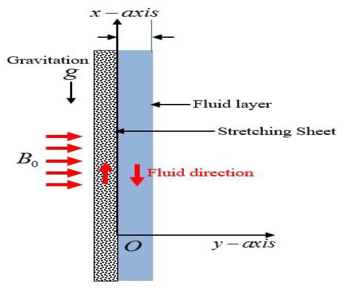
3. Mathematical Formulation
Physical Quantities
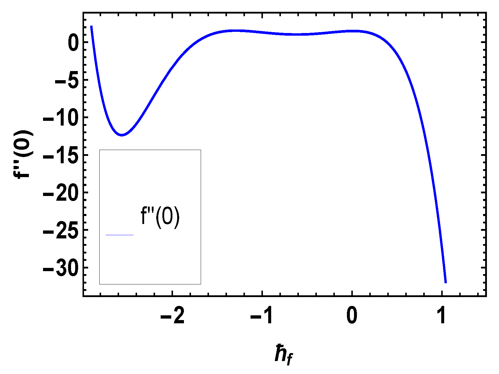
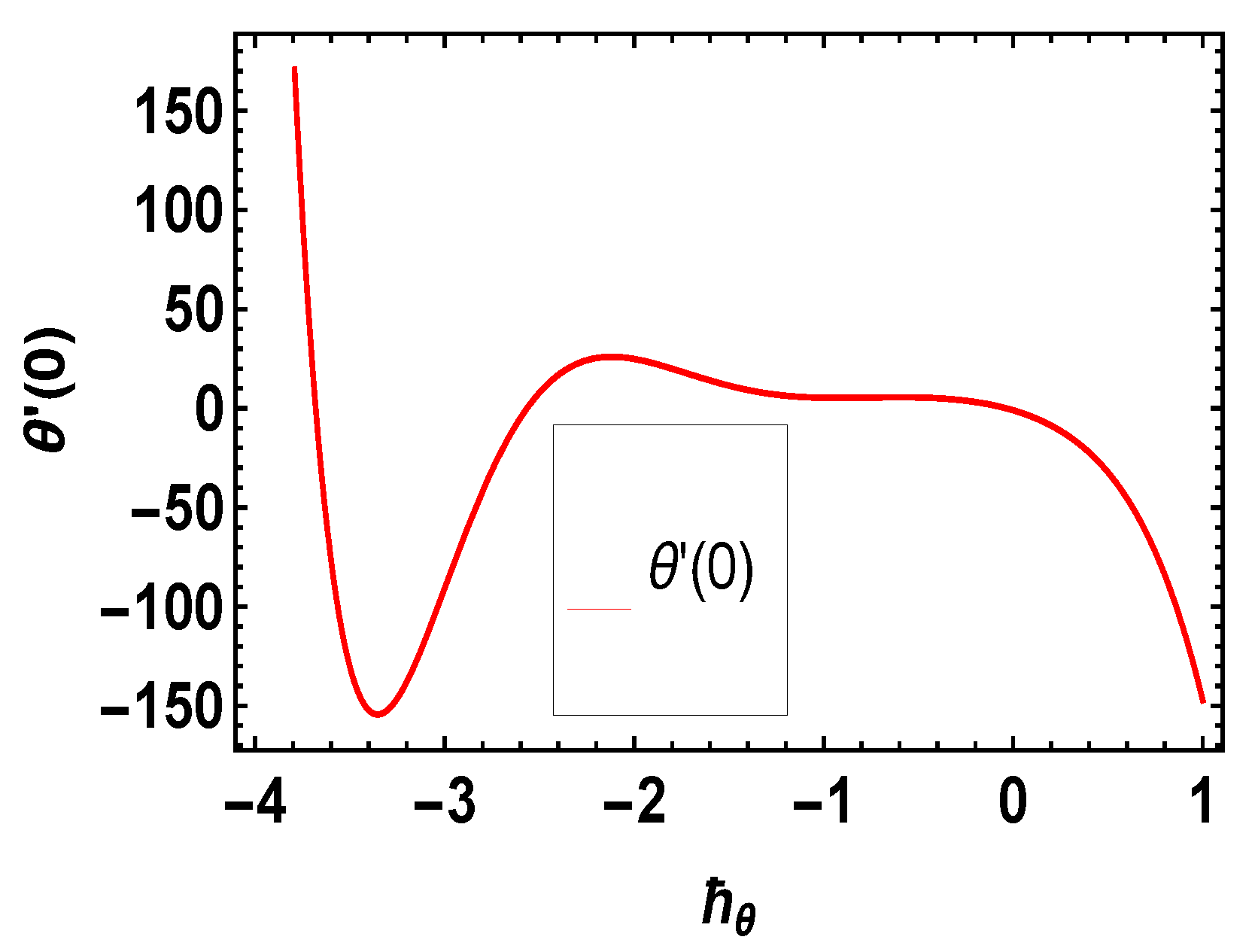
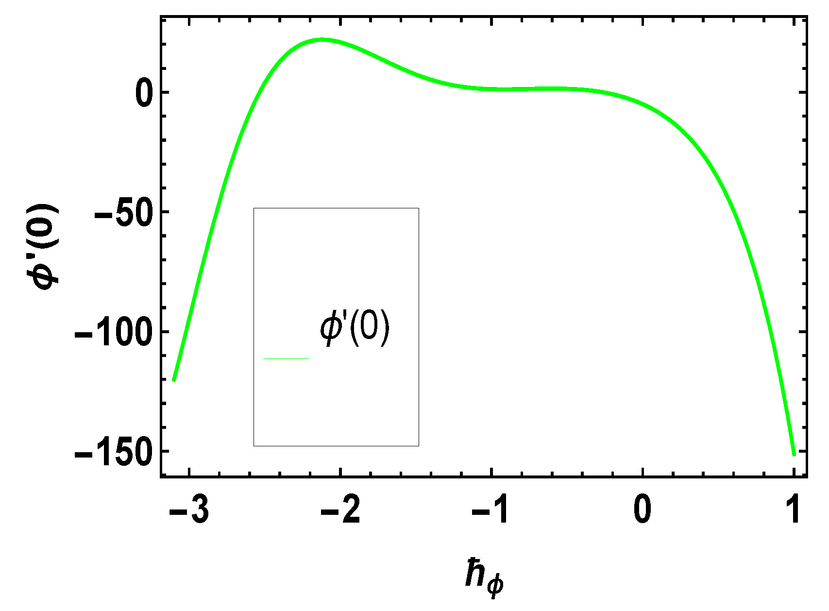
4. The HAM Solution
5. Results and Discussion
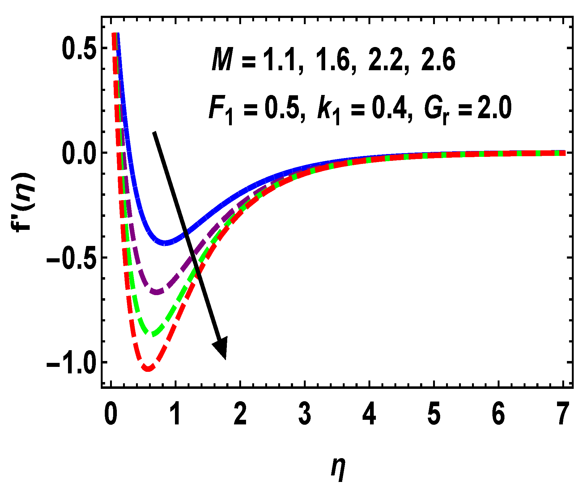
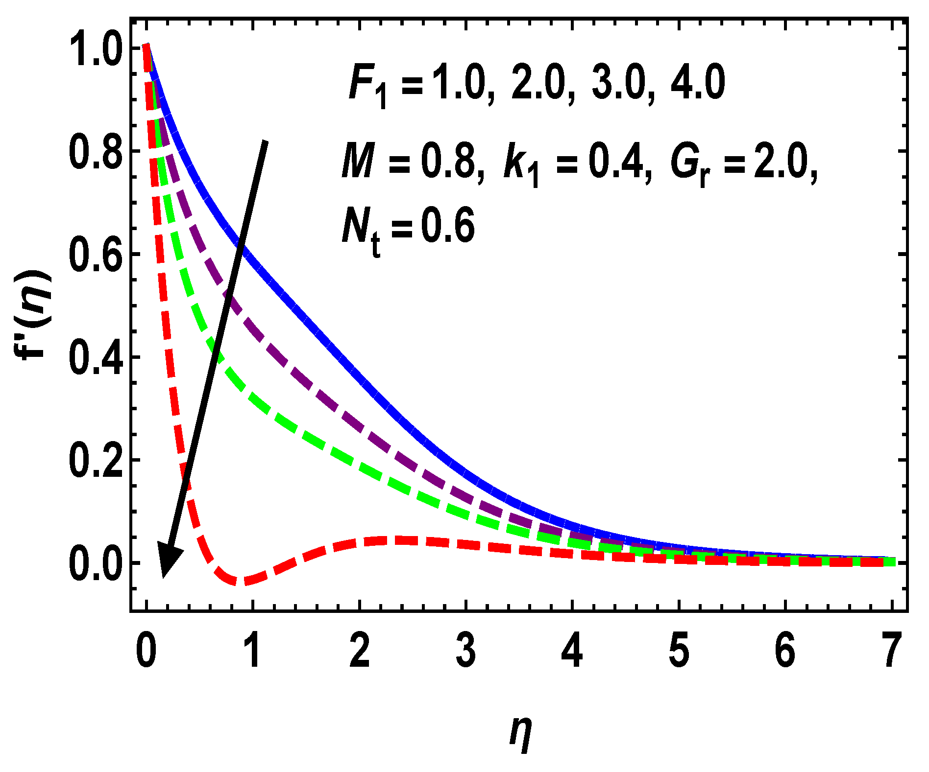
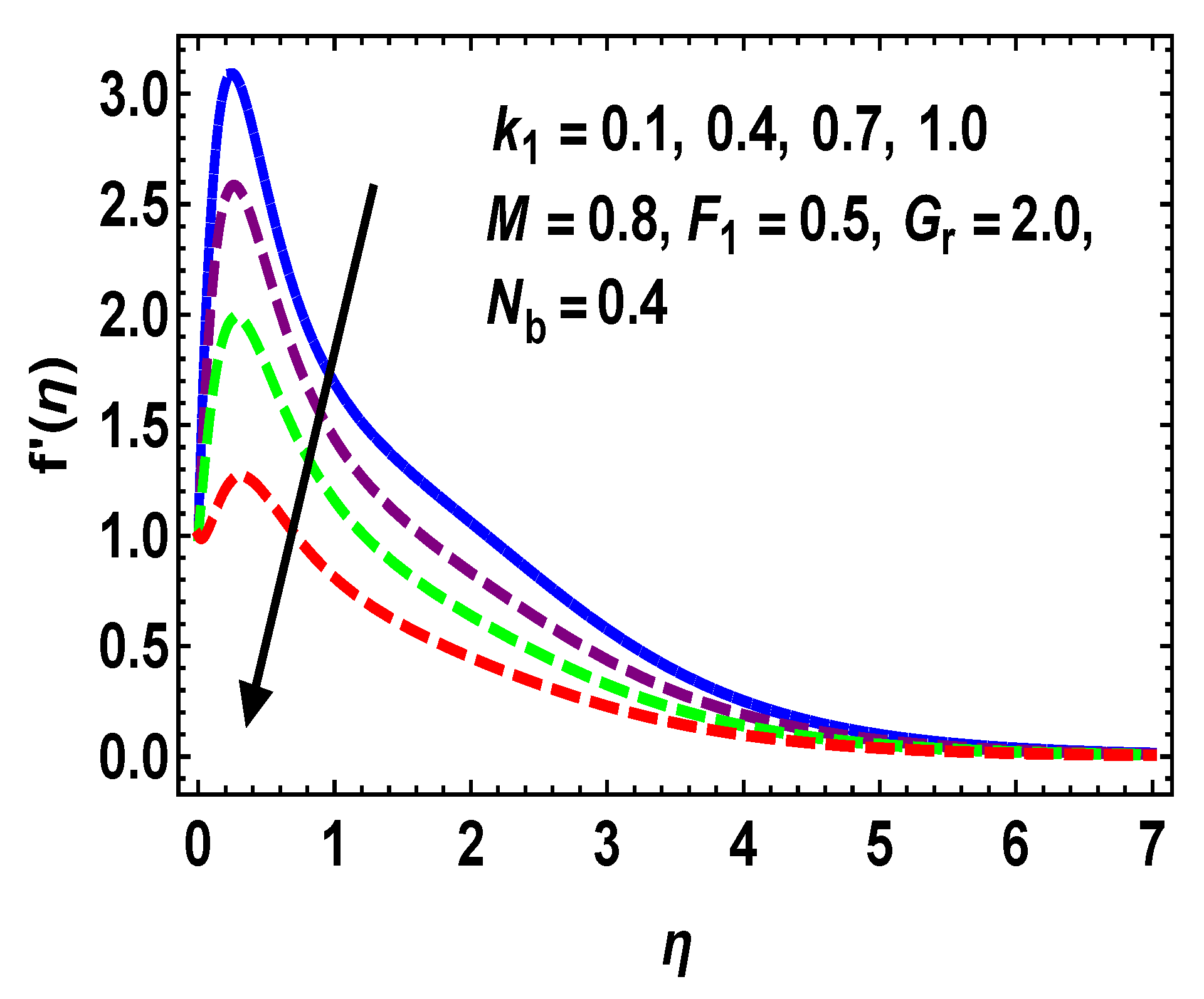
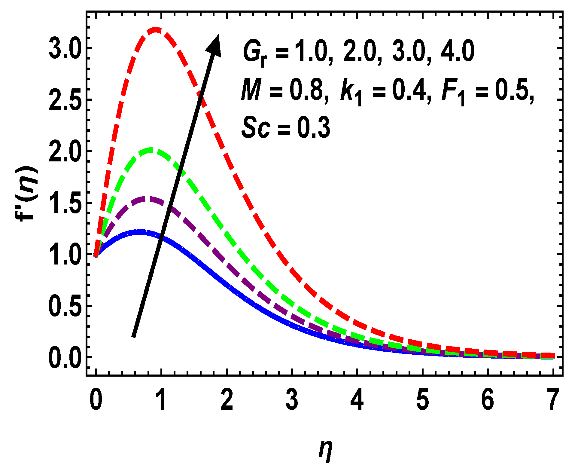
5.1. Velocity Profile
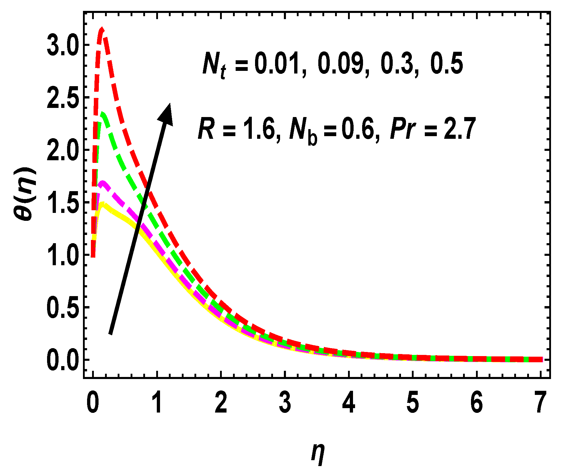
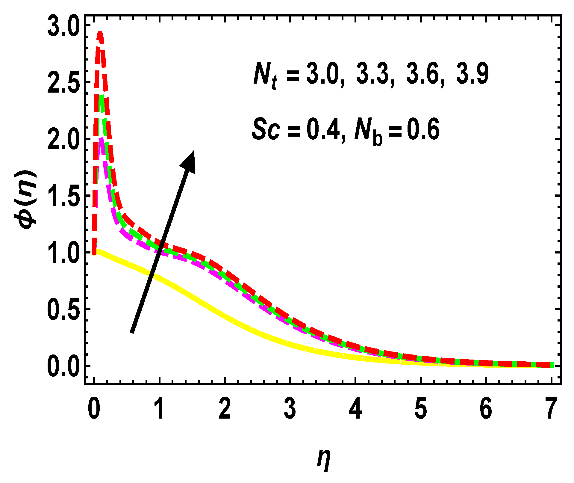
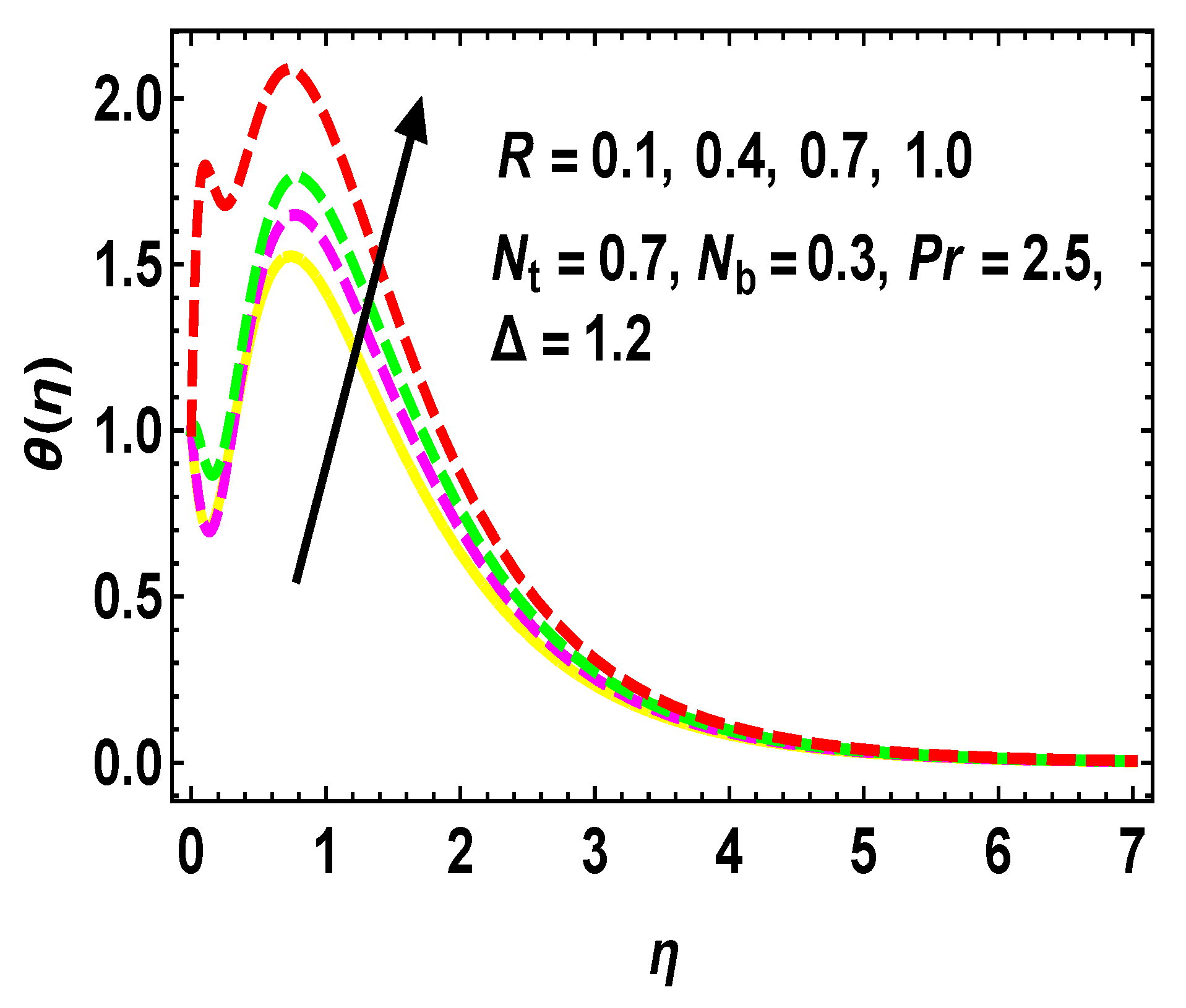
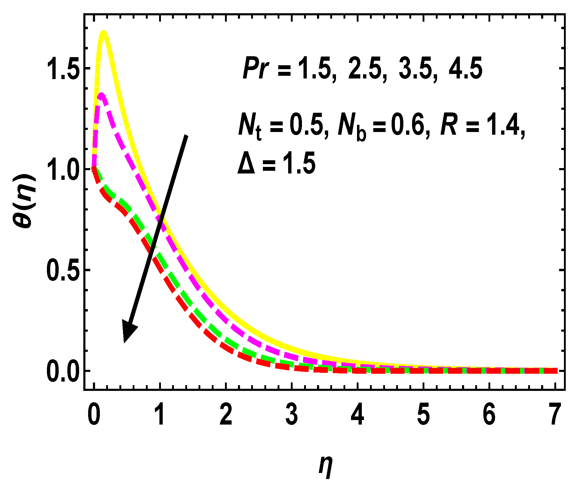
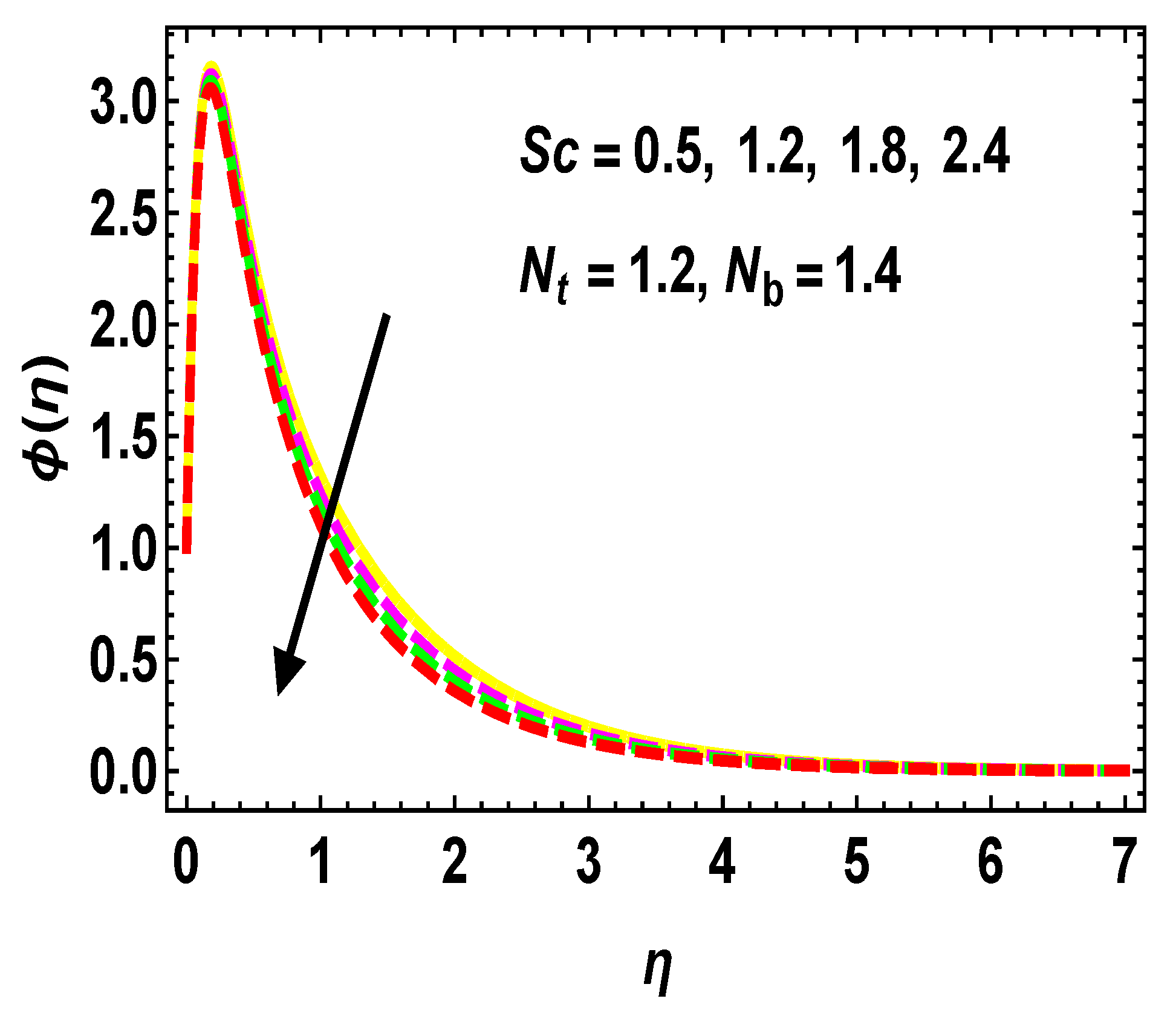
5.2. Thermal and Concentration Profiles
5.3. Table Discussions
6. Concluding Remarks
- increased for high values of and decreased for the increment values of , , and M.
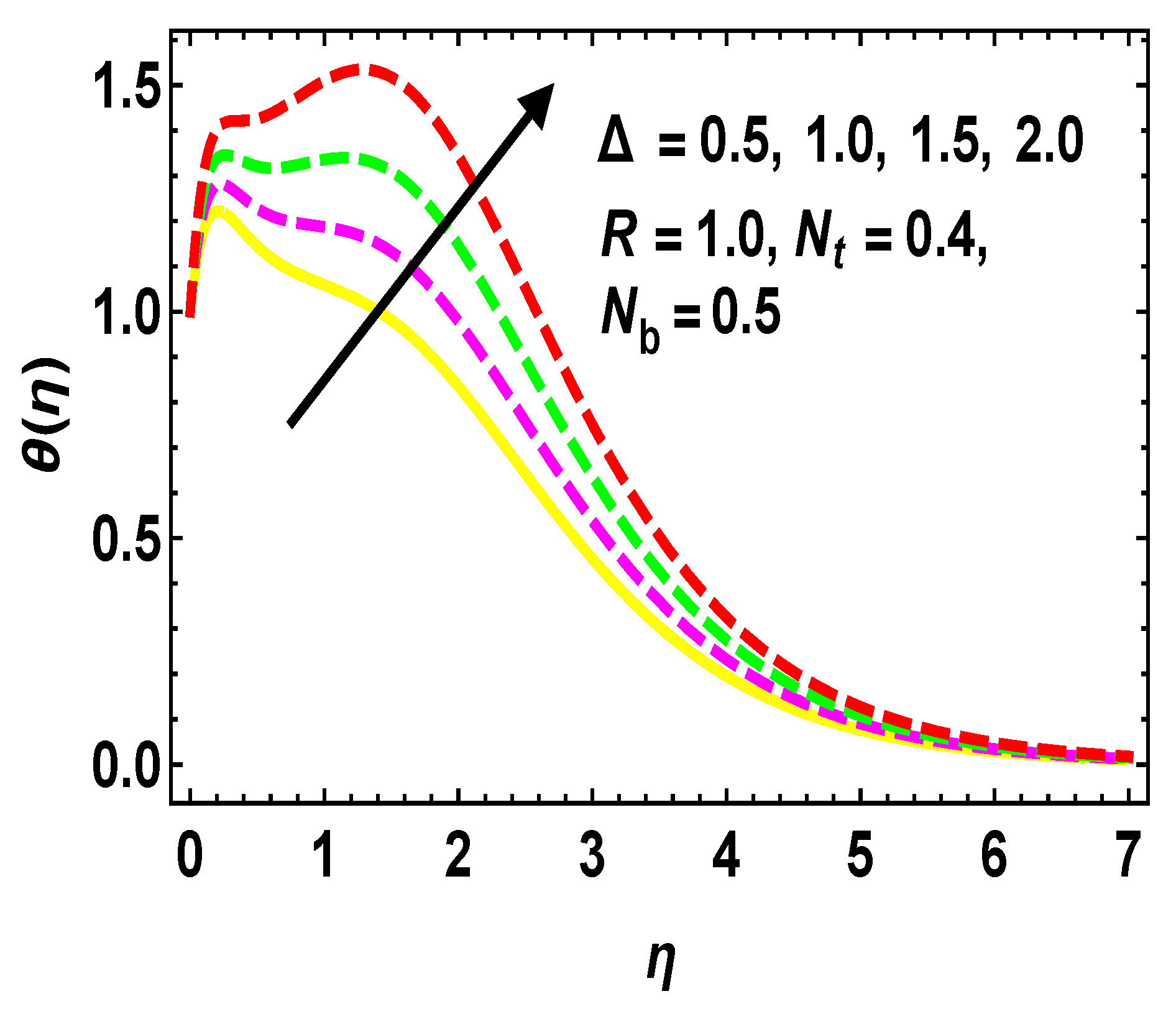
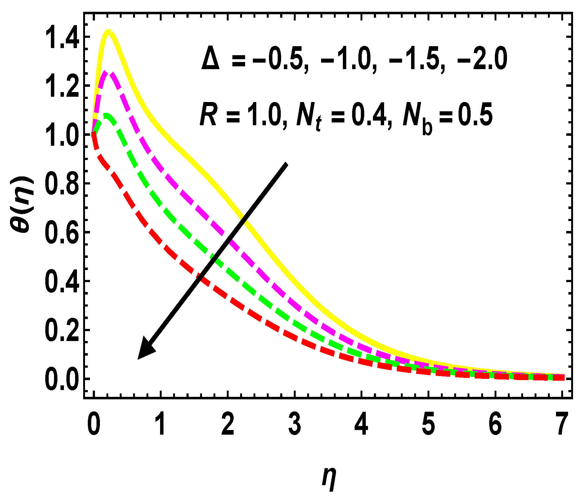
- enhances with the rising rates of , , R, and , and diminishes with higher and negative values of .
- For more estimations of , there is an increment in the curves.
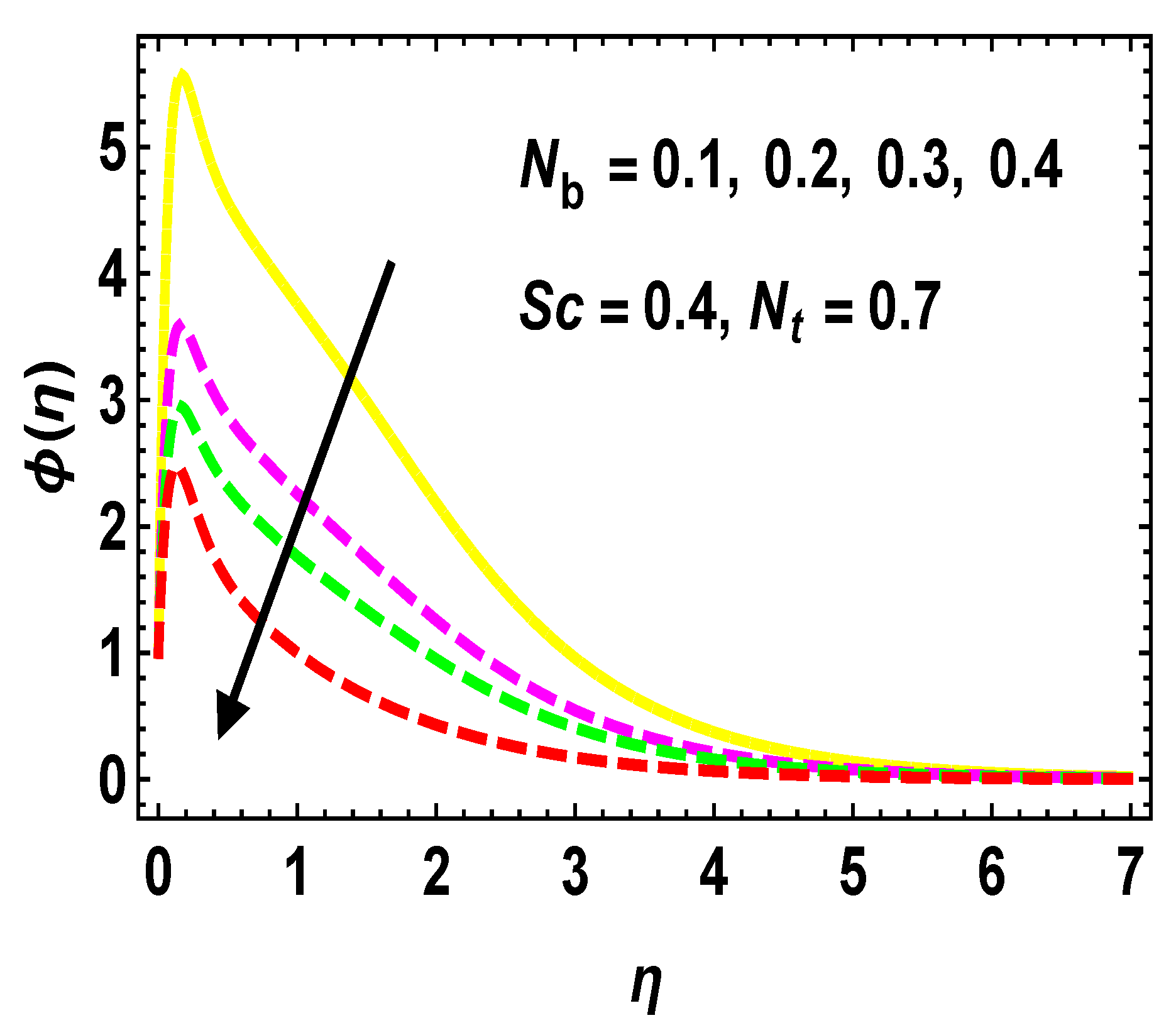
- gradually diminishes against higher values of and .
- Higher estimations of M, , and upsurge , whereas the reverse is seen for .
- enhances due to increments of , R and , while it reduces due to higher values.
- reduces due to greater estimation of and decreases for higher values of and .
- The role of the Grashof number is the same in free convection as that of the Reynolds number in the forced convection.
Author Contributions
Funding
Data Availability Statement
Conflicts of Interest
Nomenclature
| applied magnetic induction | |
| stretching rate | |
| thermophoresis parameter | |
| v, u | velocity components along y and x direction (ms) |
| T | fluid temperature (K) |
| thermal expansion | |
| similarity variable | |
| stream function (ms) | |
| free stream temperature (K) | |
| fluid density (kgm) | |
| acceleration due to gravity | |
| Boltzmann constant (WmK) | |
| specific heat (JmK) | |
| electrical conductivity | |
| heat generation/absorption | |
| thermal diffusivity | |
| M | magnetic parameter |
| mean absorption coefficient | |
| wall temperature (K) | |
| porosity parameter | |
| R | radiation parameter |
| kinematic viscosity (ms) | |
| ℏ | convergence control parameter |
| inertia parameter | |
| heat source/sink parameter | |
| Reynolds number | |
| Grashof number | |
| auxiliary linear-operator | |
| Schmidt number | |
| heat flux | |
| Prandtl number | |
| suction/injection parameter | |
| non-linear operator | |
| Brownian motion parameter |
Appendix A. Derivation of the Flow Problem
Appendix A.1. Derivation of the Continuity Equation
Appendix A.2. Derivation of the Momentum Equation
Appendix A.3. Derivation of the Energy Equation
Appendix A.4. Derivation of Concentration Equation
Appendix A.5. Derivation of Boundary Conditions
References
- Chaudhary, S.; Kumar, P. Unsteady magnetohydrodynamic boundary layer flow near the stagnation point towards a shrinking surface. J. Appl. Math. Phys. 2015, 3, 921–930. [Google Scholar] [CrossRef] [Green Version]
- Naramgari, S.; Sulochana, C. MHD flow over a permeable stretching/shrinking sheet of a nanofluid with suction/injection. Alex. Eng. J. 2016, 55, 819–827. [Google Scholar] [CrossRef] [Green Version]
- Reddy, G.V.R.; Reddy, N.B.; Gorla, R.S.R. Radiation and chemical reaction effects on MHD flow along a moving vertical porous plate. Int. J. Appl. Mech. Eng. 2016, 21, 157–168. [Google Scholar] [CrossRef] [Green Version]
- Mishra, S.R.; Jena, S. Numerical solution of boundary layer MHD flow with viscous dissipation. Sci. World J. 2014, 2014, 756498. [Google Scholar] [CrossRef]
- Babu, P.R.; Rao, J.A.; Sheri, S. Radiation effect on MHD heat and mass transfer flow over a shrinking sheet with mass suction. J. Appl. Fluid Mech. 2014, 7, 641–650. [Google Scholar] [CrossRef]
- Mabood, F.; Khan, W.A.; Ismail, A.M. MHD flow over exponential radiating stretching sheet using homotopy analysis method. J. King Saud Univ. Eng. Sci. 2017, 29, 68–74. [Google Scholar] [CrossRef]
- Pal, D.; Mondal, H. Effect of variable viscosity on MHD non-Darcy mixed convective heat transfer over a stretching sheet embedded in a porous medium with non-uniform heat source/sink. Commun. Nonlinear. Sci. Numer. Simul. 2010, 15, 1553–1564. [Google Scholar] [CrossRef]
- Zeeshan, A.; Ellahi, R.; Hassan, M. Magnetohydrodynamic flow of water/ethylene glycol based nanofluids with natural convection through a porous medium. Eur. Phys. J. Plus 2014, 129, 261. [Google Scholar] [CrossRef]
- Mahmoud, M.A.A. Variable viscosity effects on hydromagnetic boundary. Appl. Math. Sci. 2017, 1, 799–814. [Google Scholar]
- Kishore, P.M.; Rajesh, V.; Verma, V.S. The effects of thermal radiation and viscous dissipation on MHD heat and mass diffusion flow past an oscillating vertical plate embedded in a porous medium with variable surface conditions. Theor. Appl. Mech. 2012, 39, 99–125. [Google Scholar] [CrossRef]
- Majeed, A.; Noori, F.M.; Zeeshan, A.; Mahmood, T.; Rehman, S.U.; Khan, I. Analysis of activation energy in magnetohydrodynamic flow with chemical reaction and second order momentum slip model. Case Stud. Therm. Eng. 2018, 12, 765–773. [Google Scholar] [CrossRef]
- Sharma, R.; Ishak, A.; Nazar, R.; Pop, I. Boundary layer flow and heat transfer over a permeable exponentially shrinking sheet in the presence of thermal radiation and partial slip. J. Appl. Fluid Mech. 2014, 7, 125–134. [Google Scholar] [CrossRef]
- Poornima, T.; Reddy, N.B. Radiation effects on mhd free convective boundary layer flow of nanofluids over a nonlinear stretching sheet. Adv. Appl. Sci. Res. 2013, 4, 190–202. [Google Scholar]
- Singh, P.; Jangid, A.; Tomer, N.S.; Sinha, D. Effects of thermal radiation and magnetic field on unsteady stretching permeable sheet in presence of free stream velocity. Int. J. Phys. Math. Sci. 2010, 4, 396–402. [Google Scholar]
- Ahmad, I.; Sajid, M.; Awan, W.; Rafique, M.; Aziz, W.; Ahmed, M.; Abbasi, A.; Taj, M. MHD flow of a viscous fluid over an exponentially stretching sheet in a porous medium. J. Appl. Math. 2014, 2014, 256761. [Google Scholar] [CrossRef] [Green Version]
- Shateyi, S.; Motsa, S.S. Thermal radiation effects on heat and mass transfer over an unsteady stretching surface. Math. Probl. Eng. 2009, 2009, 965603. [Google Scholar] [CrossRef] [Green Version]
- Waheed, S.E. Flow and heat transfer in a maxwell liquid film over an unsteady stretching sheet in a porous medium with radiation. SpringerPlus 2016, 5, 1061. [Google Scholar] [CrossRef] [Green Version]
- Khan, A.S.; Nie, Y.; Shah, Z. Impact of thermal radiation on magnetohydrodynamic unsteady thin film flow of Sisko fluid over a stretching surface. Process 2016, 7, 369. [Google Scholar] [CrossRef] [Green Version]
- Metri, P.G.; Tawade, J.; Abel, M.S. Thin film flow and heat transfer over an unsteady stretching sheet with thermal radiation. arXiv 2016, arXiv:1603.03664. [Google Scholar]
- Khan, Z.; Srivastava, H.M.; Mohammed, P.O.; Jawad, M.; Jan, R.; Nonlaopon, K. Thermal boundary layer analysis of MHD nanofluids across a thin needle using non-linear thermal radiation. Math. Biosci. Eng. 2022, 19, 14116–14141. [Google Scholar] [CrossRef]
- Garia, R.; Rawat, S.K.; Kumar, M.; Yaseen, M. Hybrid nanofluid flow over two different geometries with Cattaneo–Christov heat flux model and heat generation: A model with correlation coefficient and probable error. Chin. J. Phys. 2021, 74, 421–439. [Google Scholar] [CrossRef]
- Garia, R.; Rawat, S.K.; Kumar, M.; Yaseen, M. Cattaneo–Christov heat flux model in Darcy–Forchheimer radiative flow of MoS2–SiO2/kerosene oil between two parallel rotating disks. J. Therm. Anal. Calorim. 2022, 147, 10865–10887. [Google Scholar] [CrossRef]
- Khan, Z.; Jawad, M.; Bonyah, E.; Khan, N.; Jan, R. Magnetohydrodynamic thin film flow through a porous stretching sheet with the impact of thermal radiation and viscous dissipation. Math. Probl. Eng. 2022, 2022, 1086847. [Google Scholar] [CrossRef]
- Jawad, M.; Khan, Z.; Bonyah, E.; Jan, R. Analysis of hybrid nanofluid stagnation point flow over a stretching surface with melting heat transfer. Math. Probl. Eng. 2022, 2022, 9469164. [Google Scholar] [CrossRef]
- Dullien, F.A.L. Porous Media: Fluid Transport and Pore Structure, 2nd ed.; Academic Press: New York, NY, USA; London, UK; San Diego, CA, USA, 2012. [Google Scholar]
- Nield, D.A.; Bejan, A. Convection in Porous Media, 5th ed.; Springer: Berlin/Heidelberg, Germany; New York, NY, USA, 2006. [Google Scholar] [CrossRef]
- Karniadakis, G.E.M.; Beskok, A.; Gad-el-Hak, M. Micro flows: Fundamentals and simulation. Appl. Mech. Rev. 2002, 55, B76. [Google Scholar] [CrossRef]
- Hussain, A.; Muneer, Z.; Malik, M.Y.; Ali, S. Formulating the behavior of thermal radiation and magnetic dipole effects on Darcy-Forchheimer grasped ferrofluid flow. Canad. J. Phys. 2019, 97, 938–949. [Google Scholar] [CrossRef]
- Forchheimer, P. Wasserbewegung durch boden. Z. Ver. Deutsch. Ing. 1901, 45, 1782–1788. [Google Scholar]
- Pal, D.; Mondal, H. Hydromagnetic convective diffusion of species in Darcy—Forchheimer porous medium with non-uniform heat source/sink and variable viscosity. Int. Commun. Heat Mass Transf. 2012, 39, 913–917. [Google Scholar] [CrossRef]
- Ganesh, N.V.; Hakeem, A.K.A.; Ganga, B. Darcy–Forchheimer flow of hydromagnetic nanofluid over a stretching/shrinking sheet in a thermally stratified porous medium with second order slip, viscous and Ohmic dissipations effects. Ain Shams Eng. J. 2018, 9, 939–951. [Google Scholar] [CrossRef] [Green Version]
- Seth, G.S.; Mandal, P.K. Hydromagnetic rotating flow of Casson fluid in Darcy-Forchheimer porous medium. MATEC Web Conf. 2018, 192, 02059. [Google Scholar] [CrossRef] [Green Version]
- Seddeek, M.A. Influence of viscous dissipation and thermophoresis on Darcy–Forchheimer mixed convection in a fluid saturated porous media. J. Colloid Interface Sci. 2006, 293, 137–142. [Google Scholar] [CrossRef]
- Hayat, T.; Muhammad, T.; Mezal, S.A.; Liao, S.J. Darcy-forchheimer flow with variable thermal conductivity and Cattaneo–Christov heat flux. Int. J. Numer. Methods Heat Fluid Flow 2006, 26, 2355–2369. [Google Scholar] [CrossRef]
- Rajesh, V.; Sheremet, M.A.; Öztop, H.F. Impact of hybrid nanofluids on MHD flow and heat transfer near a vertical plate with ramped wall temperature. Case Stud. Therm. Eng. 2021, 28, 101557. [Google Scholar] [CrossRef]
- Yaseen, M.; Rawat, S.K.; Shafiq, A.; Kumar, M.; Nonlaopon, K. Analysis of heat transfer of mono and hybrid nanofluid flow between two parallel plates in a Darcy porous medium with thermal radiation and heat generation/absorption. Symmetry 2022, 14, 1943. [Google Scholar] [CrossRef]
- Raza, R.; Naz, R.; Abdelsalam, S.I. Microorganisms swimming through radiative Sutterby nanofluid over stretchable cylinder: Hydrodynamic effect. Numer. Methods Partial. Differ. Equ. 2022, 1–20. [Google Scholar] [CrossRef]
- Faizan, M.; Ali, F.; Loganathan, K.; Zaib, A.; Reddy, C.A.; Abdelsalam, S.I. Entropy Analysis of Sutterby Nanofluid Flow over a Riga Sheet with Gyrotactic Microorganisms and Cattaneo–Christov Double Diffusion. Mathematics 2022, 10, 3157. [Google Scholar] [CrossRef]
- Bhattacharyya, K. Effects of radiation and heat source/sink on unsteady MHD boundary layer flow and heat transfer over a shrinking sheet with suction/injection. Front. Chem. Sci. Eng. 2011, 5, 376–384. [Google Scholar] [CrossRef]
- Mukhopadhyay, S. Slip effects on MHD boundary layer flow over an exponentially stretching sheet with suction/blowing and thermal radiation. Ain Shams Eng. J. 2013, 4, 485–491. [Google Scholar] [CrossRef] [Green Version]
- Marin, M.; Öchsner, A. The effect of a dipolar structure on the Hölder stability in Green-Naghdi thermoelasticity. Contin. Mech. Thermodyn. 2017, 29, 1365–1374. [Google Scholar] [CrossRef]
- Marin, M. Cesaro means in thermoelasticity of dipolar bodies. Acta Mech. 1997, 122, 155–168. [Google Scholar] [CrossRef]
- Liao, S. The Proposed Homotopy Analysis Technique for the Solution of Nonlinear Problems. Ph.D. Thesis, Shanghai Jiao Tong University, Shanghai, China, 1992. [Google Scholar]
- Liao, S. A kind of approximate solution technique which does not depend upon small parameters. II. An application in fluid mechanics. Int. J. Nonlinear Mech. 1997, 32, 815–822. [Google Scholar] [CrossRef]
- Liao, S. On the analytic solution of magnetohydrodynamic flows of non-Newtonian fluids over a stretching sheet. J. Fluid Mech. 2003, 488, 189–212. [Google Scholar] [CrossRef] [Green Version]
- Liao, S. A new branch of solutions of boundary-layer flows over an impermeable stretched plate. Int. J. Heat Mass Transf. 2005, 48, 2529–2539. [Google Scholar] [CrossRef]
- Liao, S. An optimal homotopy-analysis approach for strongly nonlinear differential equations. Commun. Nonlinear Sci. Numer. Simul. 2010, 15, 2003–2016. [Google Scholar] [CrossRef]
- Liao, S.; Tan, Y. A general approach to obtain series solutions of nonlinear differential equations. Stud. Appl. Math. 2007, 119, 297–354. [Google Scholar] [CrossRef]
- Daniel, Y.S.; Daniel, S.K. Effects of buoyancy and thermal radiation on MHD flow over a stretching porous sheet using homotopy analysis method. Alex. Eng. J. 2015, 54, 705–712. [Google Scholar] [CrossRef] [Green Version]
- Chamkha, A.J. Thermal radiation and buoyancy effects on hydromagnetic flow over an accelerating permeable surface with heat source or sink. Int. J. Eng. Sci. 2000, 38, 1699–1712. [Google Scholar] [CrossRef]


| 0.2 | 0.1 | 0.3 | 2.45038307 |
| 0.4 | 2.36012785 | ||
| 0.6 | 2.34056085 | ||
| 0.8 | 2.31059187 | ||
| 0.1 | 2.26205129 | ||
| 0.3 | 2.27140738 | ||
| 0.5 | 2.29025809 | ||
| 0.7 | 2.29506702 | ||
| 0.3 | 2.46230876 | ||
| 0.5 | 2.45037182 | ||
| 0.7 | 2.44570887 | ||
| 0.9 | 2.42071925 |
| M | ||||
|---|---|---|---|---|
| 0.3 | 0.1 | 0.3 | 1.0 | 1.63205892 |
| 0.4 | 1.64218038 | |||
| 0.5 | 1.64575398 | |||
| 0.6 | 1.66094124 | |||
| 0.1 | 1.23056802 | |||
| 0.2 | 1.24059735 | |||
| 0.3 | 1.25192114 | |||
| 0.4 | 1.25602565 | |||
| 0.3 | 1.43271729 | |||
| 0.5 | 1.45952172 | |||
| 0.8 | 1.47062175 | |||
| 1.0 | 1.48073426 | |||
| 1.0 | 2.03968538 | |||
| 2.0 | 1.90250917 | |||
| 3.0 | 1.86620846 | |||
| 4.0 | 1.80911127 |
| R | ||||
|---|---|---|---|---|
| 0.5 | 2.5 | 0.1 | 0.2 | 2.53802156 |
| 1.0 | 2.52508295 | |||
| 1.2 | 2.51862063 | |||
| 1.5 | 2.50752047 | |||
| 2.5 | 1.54531398 | |||
| 3.5 | 1.59370589 | |||
| 4.5 | 1.64950842 | |||
| 5.5 | 1.66097014 | |||
| 0.2 | 1.10459009 | |||
| 0.4 | 1.02054179 | |||
| 0.6 | 0.85628206 | |||
| 0.8 | 0.80049531 | |||
| 0.3 | 1.27353338 | |||
| 0.5 | 1.25904107 | |||
| 0.7 | 1.23718056 | |||
| 0.9 | 1.21562169 |
Disclaimer/Publisher’s Note: The statements, opinions and data contained in all publications are solely those of the individual author(s) and contributor(s) and not of MDPI and/or the editor(s). MDPI and/or the editor(s) disclaim responsibility for any injury to people or property resulting from any ideas, methods, instructions or products referred to in the content. |
© 2022 by the authors. Licensee MDPI, Basel, Switzerland. This article is an open access article distributed under the terms and conditions of the Creative Commons Attribution (CC BY) license (https://creativecommons.org/licenses/by/4.0/).
Share and Cite
Srivastava, H.M.; Khan, Z.; Mohammed, P.O.; Al-Sarairah, E.; Jawad, M.; Jan, R. Heat Transfer of Buoyancy and Radiation on the Free Convection Boundary Layer MHD Flow across a Stretchable Porous Sheet. Energies 2023, 16, 58. https://doi.org/10.3390/en16010058
Srivastava HM, Khan Z, Mohammed PO, Al-Sarairah E, Jawad M, Jan R. Heat Transfer of Buoyancy and Radiation on the Free Convection Boundary Layer MHD Flow across a Stretchable Porous Sheet. Energies. 2023; 16(1):58. https://doi.org/10.3390/en16010058
Chicago/Turabian StyleSrivastava, Hari Mohan, Ziad Khan, Pshtiwan Othman Mohammed, Eman Al-Sarairah, Muhammad Jawad, and Rashid Jan. 2023. "Heat Transfer of Buoyancy and Radiation on the Free Convection Boundary Layer MHD Flow across a Stretchable Porous Sheet" Energies 16, no. 1: 58. https://doi.org/10.3390/en16010058