On the Effect of the Time Interval Base and Home Appliance on the Renewable Quota of a Building in an Alpine Location

Abstract

The European goal of decarbonization drives design toward high-performance buildings that maximize the use of renewable sources. Therefore, the European RED II Directive and Italian law raise the minimum renewable share required for new buildings and major renovations. Currently, the renewable energy ratio (RER) is used for the mandatory verification, obtained with a quasi-steady state calculation on a monthly basis, while much of the scientific literature uses self-consumption factor (SCF) and load coverage factor (LCF) often calculated through dynamic simulation. However, the use of a monthly balance implies the use of the national grid as a virtual battery through the net metering mechanism. The actual share of renewable coverage in the absence of expensive electric storage will necessarily be lower. The link between the different indices, the effect of the time base used in the calculation as well as the actual renewable share achieved by buildings, considering also plug loads not in the regulatory verification framework, are still open issues. This work analyzes the actual renewable share achievable for a new building in a heating-dominated climate, i.e., the mountainous area of the municipality of Trento. The renewable share is evaluated through a coupled dynamic simulation of the building and the energy systems. The results show that the RER decreases by 13% and 15% when switching from monthly to instantaneous balance in the case without and with additional home appliance loads, respectively. Similarly, simulations show how the time interval base affects the difference between the RER index and the LCF of PV energy.

1. Introduction

The International Energy Agency [1] states that buildings’ lifecycles are responsible, directly and indirectly, for about 37% of global energy and process-related CO₂ emissions. In addition, the EU’s energy dependency has increased from 50% in 1990 to 60% in 2019, reaching 96.8% on oil and natural gas liquids and 89.7% on natural gas [2]. Moreover, there is a higher penetration of renewables and nuclear for power generation (61.2%) than for heating (30.2%) in Europe [2], and this motivates the progressive electrification of building air conditioning systems. A study by D’Agostino and Parker [3] demonstrated the key role of renewable sources in reaching the nZEB target in 12 European capitals, and this motivates the phased-in legal obligation to install PV under the REPowerEU plan [4]. According to the European Directive 2018/2001 [5], the REPowerEU Plan [4] and the Italian Legislative Decree n.199/2021 [6], heat pump and PV systems seem to be the most efficient and cost-effective solutions for reducing buildings’ carbon footprint. Nonetheless, in the absence of electric batteries, the mismatch between the solar availability and the building energy demand is one of the main challenges to be faced to achieve a high renewable share.

Different solutions have been studied in the literature to increase the renewable quota of the system, such as energy storage and control strategies to match the building load to the solar availability [7,8]. In [9], the authors showed how the use of simple rule-based controls can lead to the reduction of up to 17% of the energy withdrawn from the grid. Savolainen and Lahdelma [10] study optimized control by managing thermal storage and batteries on the basis on the coming 15 min power balance settlement. Amato et al. [11] and Kotarela et al. [12] demonstrate that the local use of photovoltaic energy can be enhanced thanks to batteries and local energy sharing, to obtain self-sufficient buildings, near to nZEB parameters. Similarly, in [13,14], the benefit of renewable energy communities in the self-consumption (SCF) of PV production emerges.

Another important issue concerns the definition of an effective index and a minimum threshold to quantify the renewable share in new construction and major renovations. The Renewable Energy Directive gives only a framework for national implementation of minimum thresholds. Several Member States require a minimum renewable energy ratio (RER) based on the primary energy [15] while the load coverage factor (LCF) defined on the share of delivered energy is often used in the literature. The renewable energy ratio (RER) was initially proposed by Kurnitski [16] and is based on the annual primary energy used, estimated with a monthly simulation of energy consumption and renewable harvesting. This implies the use of the national grid as a virtual battery through the net metering mechanism. The actual renewable share will necessarily be lower without an expensive electric storage system. However, the link between the RER estimated from the monthly balance and the RER based on the actual self-consumption of PV power in the absence of batteries is still unclear. How sensitive is the RER index to the time base used to close the energy balance? How does the renewable share calculated on primary energy rather than delivered energy vary?

A further important question is to what extent does the territory affect the renewable share? For example, the analysis of two Italian dataset of building energy certificates from Lombardy and Trentino shows how the distributions of RER are very different (Figure 1). Lombardy is mainly characterized by flat land and a less harsh climate than Trentino. Besides, the use of wood-fired boilers is prohibited in many settlements in Lombardy. This is in evident contrast with Trentino, where the use of biomass leads to a binomial distribution of the RER index. Is the wide use of wood-fired boilers related to technical limitations of the HP and PV combination in the mountainous context that makes the target on the minimum RER value difficult to achieve?

The additional question is, then, to what extent the colder climate combined with the lower availability of solar radiation due to the orography can affect the RER and PV self-consumption? Can the combination of PV and ASHP progressively replace wood boilers by ensuring adequate renewable share even in a mountainous area with a severe climate?

Furthermore, in the European context, the RER in residential buildings is calculated on the energy required for air conditioning and ventilation of buildings, considering only the energy produced by PV used by these systems. However, the constraints aimed at improving building performance should also include the share related to plug loads and especially to household appliances. In this regard, Tostado-Veliz [17] highlights the importance of helping home users to reduce their consumption tanks to Home Energy Management Systems. A comprehensive analysis that considers the real load profile of a building, combining the load profiles of household appliances with those for heating and domestic hot water, has already been conducted by Huber et al. [18] and Cuerdo-Vilches et al. [19]. However, to the best of our knowledge, the link between the RER index and the actual index including the PV energy self-consumed by the equipment has not yet been analyzed in the literature.

In order to fill these gaps, this work focuses on the analysis of a new residential building equipped with a low temperature heating system, thermal storage and a heat pump coupled with a PV system. The single-family building (MF) analyzed represents a typical Italian building [20], whose thermal properties meet mandatory constraints for new construction or major renovations.

Some patterns of equipment consumption were generated starting from the probability distributions proposed in Besagni et al. [21] and consumption profiles of major household collected during an experimental campaign. This paper aims to assess how much the appliance consumption as well as the different time interval base of the energy balance affect the calculation of the renewable share and self-consumption.

2. Materials and Methods

2.1. Experimental Monitoring of Household Appliance Profiles

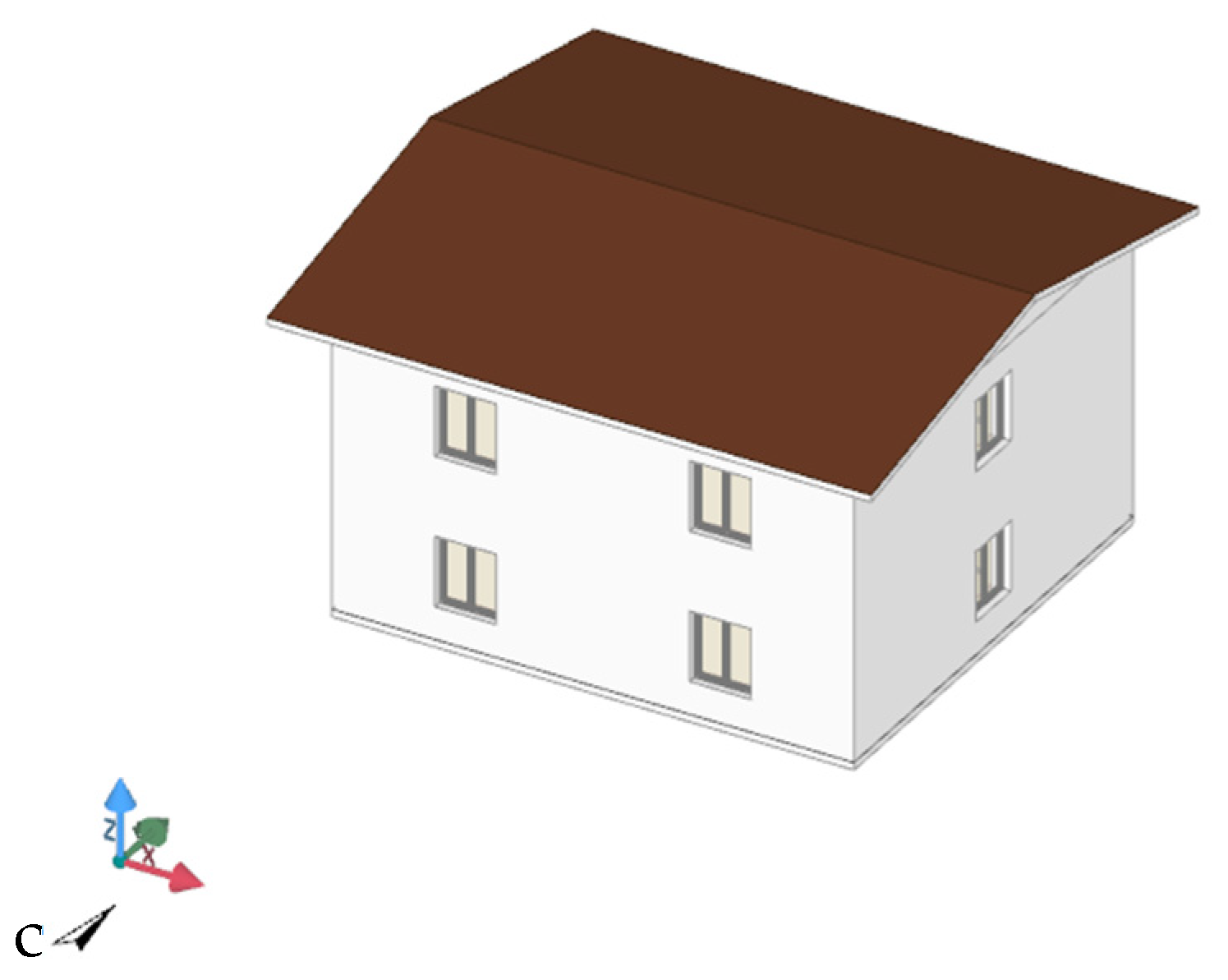
Besagni et al. [21] monitored the energy meters installed in 67 Italian households with different sociodemographic characteristics. The main results are a series of probability distributions that can represent the habits of Italian householders classified into 5 clusters with reference to the pattern of operation of major household appliances. Specifically, clusters 1 and 2 represent households with one or more children, or childless couples, aged 18 to 34 years. The first cluster relates to dwellings with a floor area of less than 146 square meters, and the second with a floor area of more than 146 square meters. The third and fourth clusters represent childless couples or single parents; cluster 3 for dwellings of less than 152 square meters, cluster 6 for more than 152 square meters. The last one (cluster 7) represents houses inhabited by a single person with an area of less than 124 square meters.

The first step of the analysis is aimed at measuring the profiles of new appliances with high energy labels according to major operating programs. The monitored appliances represent the main plug loads in an Italian residential building. Given the target of new buildings or major renovations, appliances with good performance in accordance with the European energy label were used (

Table 1. Experimental tests conducted to evaluate the withdrawal profiles of household appliances.

Household	Nominal Power [W]	EU Label (Directive 2010/30/EU)	Rated Consumption (kWh y−1)	Program	Code
Induction Hob	3700	n.a.	n.a.	Breakfast	T1
				First Course	T2
				Second Course	T3
Oven	2780	A	0.89 per Cycle	Cooking 180 °C	T4
				Heating food 180 °C	T5
Washing machine	2200	A+++	169	40 °C and 800 rpm spinning	T6
Dishwasher	2200	A++	262	Eco 50 °C	T7
				Auto 40–60 °C	T8
				High 70 °C	T9
Base load	n.a.	A+	297	Refrigerator	T10
	n.a.	A++	207	Freezer
	n.a.	n.a.	n.a.	modem and TV standby
Dryer machine	700	A+++	176	Cottons	T11

). In contrast to other work, the refrigerator and freezer were monitored and included in the base load of the building, since their electrical consumption seems to be less affected by users.

Data were collected with a timestep of 1 min by building a low-cost system obtained by interfacing a Raspberry PI 3 to a Fronius 63A energy meter via Modbus protocol. The energy meter belongs to class B according to EN 50470 [22] and thus has an accuracy of less than 1% on active power while it is a class 2 according to the EN/IEC 62053 [23] standard for reactive power measurement.

Typical uses of the appliances shown in Table 1 have been tested. The purpose is to determine not only the consumption but also the different time duration of energy loads. A custom Matlab code was then implemented to construct stochastic withdrawal profiles through the curves proposed in [21] and the monitored consumption experimentally derived. A contracted power of 3 kW with a 10% tolerance as usual in Italian utility contracts is used as a constraint in profile generation.

2.2. Case Study

The paper specifically analyzes the alpine climate context of northern Italy, of the municipality of Trento, in Trentino (

Table 2. Climatic data for the municipality of Trento.

Municipality	Climatic Zone	Lat	Alt	Tdesign	Tair
Trento	E	46.04 N	194 m a.s.l.	−12 °C	12.9 °C

). Trento is located in the Italian climatic zone “E”, with heating degree days from 2101 Kd to 3000 Kd [24]. Climate data are those of UNI 10349-1 standard [25].

The single-family building (Figure 2) represents a typical Italian building [20]. It is composed of 2 floors, each with an area of around 88 m². The thermal characteristics are close to the limits of transmittance required by the current local legislation [26]. To reach a high-performance level, the building has 15 cm of extruded polystyrene (EPS) insulation on the external walls, 12 cm on the roof and well-insulated windows. The thermal load calculation has been performed by splitting the building along the west to the east axis in 4 thermal zones, 44 m² each, with uniform solar gains.

Table 3. Geometrical characteristics of the single-family building.

Geometrical Characteristics	Value	Unit
Floor	2	/
Apartments	1	/
Net floor area	104.6	m2
Gross floor area	87.99	m2
Net Volume	527.91	m2
Glazing area to North	8.4	m2
Glazing area to South	8.4	m2
Glazing area to East/West	8.4	m2
Height/1 floor	3	m

and

Table 4. Thermal properties of the single-family building.

Thermal Properties	Value	Unit
Ufloor	0.37	Wm−2K−1
Uwall	0.18	Wm−2K−1
Uroof	0.23	Wm−2K−1
Uwindow	0.80	Wm−2K−1

presents the main geometrical characteristics and the thermal properties of the building.

The heating system (Figure 3) consists of an inverter-driven heat pump (HP), a buffer storage tank (BS) for space heating (SH) and a thermal energy storage (TES) for domestic hot water (DHW) preparation. The heat pump has a rated capacity of 7.18 kW with a source temperature 7 °C and a sink one 35 °C. The emission terminals for SH are radiant panels fed with an inlet temperature of the hot water of 35 °C in the design conditions (i.e., −12 °C). The supply temperature to the radiant panels, as well as the BS and the HP setpoint temperatures are controlled by an outdoor reset control. The setpoint temperature of the TES is 50 °C. The temperature of the BS and TES determine the activation of the heat pump and are controlled by a proportional control. The building is also provided with a photovoltaic system on the south pitch of the roof with a tilt angle of 20°. There are seven 420 W_p modules connected in series, resulting in a peak power of 2.94 kW and an overall area of 12 m² (i.e., roughly 12.5% of the roof surface).

The HVAC system is controlled with two different strategies. In the first scenario (bas), there is no advanced control strategy and then the heat pump is activated whenever the proportional control detects a drop of TES and BS temperatures from their setpoints. In the second scenario (enh), a rule-based control strategy (RBC) is adopted to maximize the SC of PV generation. The BS and TES set-points are raised, in case of PV energy surplus. This strategy, for inverter-driven air-to-water heat pump, is fully described in Pinamonti et al. [9]. This control algorithm controls the compressor rotational speed so that the heat pump exploits all the available PV power. The excess thermal energy is firstly stored in the TES by raising its temperature set point up to 60 °C. If the TES is fully charged, the outdoor temperature reset curve’s maximum value is raised by 10 K allowing for energy storage within the BS as well.

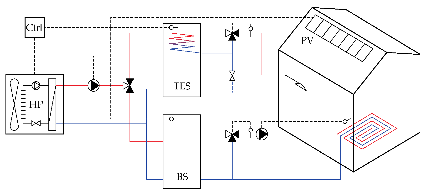
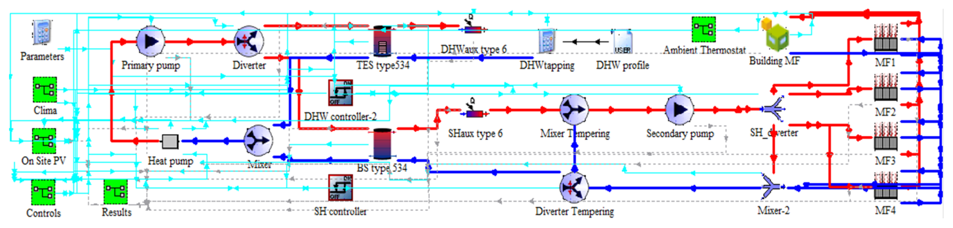
2.3. Simulation Model

The building and the HVAC systems are modelled with TRNSYS 2018, as shown in Figure 4, with a one-minute time-step. The simulations were carried out first with only heating and domestic hot water requirements, and then, with the addition of household appliance consumption. The model of the building is created using the subroutine type 56. The internal gains are set equal to 4 W m⁻², half radiative and half convective, and a constant ventilation rate of 0.3 ACH is considered. The heat pump model was developed by Bee et al. [27] and it is based on performance maps provided by a manufacturer. Part-load operation is modeled through the COP correction factor that depends on the ratio of the compressor supply frequency vs. the nominal frequency (i.e., 50 Hz)—that is a good approximation of the capacity ratio (CR). The frequency is varied to modulate the HP thermal power output according to the relationship between the frequency and the electric power absorption obtained from manufacturer data.

2.4. Key Performance Indicators

The renewable energy share is evaluated on a monthly basis although the energy simulation evaluates the power absorption with a time step of 1 min. This choice is intended to relate real energy self-sufficiency to the renewable energy ratio defined in the European regulatory framework for buildings and to the Italian standard [28]. Therefore, the monthly values of load coverage factor (LCF) and self-consumption factor (SCF) are evaluated through Equations (1) and (2). While the former gives an indication of energy self-sufficiency, the latter describes how much of the energy produced by PV is exploited. They are both calculated assessing delivered energy on the different energy carriers, and then, for the test case on electricity.

$$\mathrm{L}\mathrm{C}{\mathrm{F}}_{\mathrm{t}\mathrm{b}}=\frac{{\sum }_{\mathrm{t}\mathrm{b}}\mathrm{m}\mathrm{i}\mathrm{n}\left({\int }_{\mathrm{t}\mathrm{b}}^{}\mathrm{W};{\int }_{\mathrm{t}\mathrm{b}}^{}\mathrm{P}\mathrm{V}\right)}{{\sum }_{\mathrm{t}\mathrm{b}}{\int }_{\mathrm{t}\mathrm{b}}^{}\mathrm{W}}$$

(1)

$$\mathrm{S}\mathrm{C}{\mathrm{F}}_{\mathrm{t}\mathrm{b}}=\frac{{\sum }_{\mathrm{t}\mathrm{b}}\mathrm{m}\mathrm{i}\mathrm{n}\left({\int }_{\mathrm{t}\mathrm{b}}^{}\mathrm{W};{\int }_{\mathrm{t}\mathrm{b}}^{}\mathrm{P}\mathrm{V}\right)}{{\sum }_{\mathrm{t}\mathrm{b}}{\int }_{\mathrm{t}\mathrm{b}}^{}\mathrm{P}\mathrm{V}}$$

(2)

The term tb appears in Equations (1) and (2), which represents the time base used for closing the balance between PV energy and power absorption (W). From a physical point of view, the balance is nearly instantaneous (in our case with a tb of 1 min). However, depending on the net metering scheme, closures of the balance can be performed on an hourly or monthly basis. For this reason, the SCF and LCF indices were calculated using a tb equal to one minute, one hour or one month. Likewise, the renewable energy ratio (Equation (3)) was also calculated by employing different tb in the energy balance, although most European member states use the index calculated with monthly tb to establish the regulatory performance requirements. Unlike the LCF index, the RER is evaluated directly on primary energy and therefore, also includes the renewable thermal energy that the HP takes from the source.

$$\mathrm{R}\mathrm{E}{\mathrm{R}}_{\mathrm{t}\mathrm{b}}=\frac{{\sum }_{\mathrm{t}\mathrm{b}}\left({\mathrm{f}}_{\mathrm{P}\mathrm{V},\mathrm{r}\mathrm{e}\mathrm{n}}\mathrm{·}{\int }_{\mathrm{t}\mathrm{b}}^{}{\mathrm{W}}_{\mathrm{P}\mathrm{V}}+{\mathrm{f}}_{\mathrm{G}\mathrm{r}\mathrm{i}\mathrm{d},\mathrm{r}\mathrm{e}\mathrm{n}}\mathrm{·}{\int }_{\mathrm{t}\mathrm{b}}^{}{\mathrm{W}}_{\mathrm{G}\mathrm{r}\mathrm{i}\mathrm{d}}+{\mathrm{f}}_{\mathrm{S}\mathrm{o}\mathrm{u}\mathrm{r}\mathrm{c}\mathrm{e},\mathrm{r}\mathrm{e}\mathrm{n}}\mathrm{·}{\int }_{\mathrm{t}\mathrm{b}}^{}{\mathrm{Q}}_{\mathrm{s}\mathrm{o}\mathrm{u}\mathrm{r}\mathrm{c}\mathrm{e}}\right)}{{\sum }_{\mathrm{t}\mathrm{b}}\left({\mathrm{f}}_{\mathrm{P}\mathrm{V},\mathrm{t}\mathrm{o}\mathrm{t}}\mathrm{·}{\int }_{\mathrm{t}\mathrm{b}}^{}{\mathrm{W}}_{\mathrm{P}\mathrm{V}}+{\mathrm{f}}_{\mathrm{G}\mathrm{r}\mathrm{i}\mathrm{d},\mathrm{t}\mathrm{o}\mathrm{t}}\mathrm{·}{\int }_{\mathrm{t}\mathrm{b}}^{}{\mathrm{W}}_{\mathrm{G}\mathrm{r}\mathrm{i}\mathrm{d}}+{\mathrm{f}}_{\mathrm{S}\mathrm{o}\mathrm{u}\mathrm{r}\mathrm{c}\mathrm{e},\mathrm{t}\mathrm{o}\mathrm{t}}\mathrm{·}{\int }_{\mathrm{t}\mathrm{b}}^{}{\mathrm{Q}}_{\mathrm{s}\mathrm{o}\mathrm{u}\mathrm{r}\mathrm{c}\mathrm{e}}\right)}$$

(3)

where:

W_PV is the share of load covered by PV in the considered time-based (tb)

W_Grid is the share of load covered by electricity taken from national grid

Q_Source is the HP thermal energy taken on site from the source

f_PV,ren, f_Grid,ren, f_Source,ren are the conversion factors to renewable primary energy

f_PV,tot, f_Grid,tot, f_Source,tot are the conversion factors to primary energy, both the renewable and non-renewable shares. These coefficients are defined according to Italian regulations (

Table 5. Primary energy factors for the RER calculation.

Source/Carrier	fP,ren	fP,TOT
PV	1	1
HP source	1	1
Electricity from Grid	0.47	2.42

), but similar values are defined for other European countries.

3. Results

This section presents the results of the analysis. The first subsection illustrates the trends in the sampling profiles of household appliances measured during the experimental campaign. Next, the results of dynamic simulation are presented, for both scenarios: with the basic and the enhanced control strategy. Finally, simulations are conducted again to evaluate the influence of plug loads on the performance indices. The overall analysis performed allows to understand the extent to which a different time base (tb) affects the RER, SCF and LCF indexes.

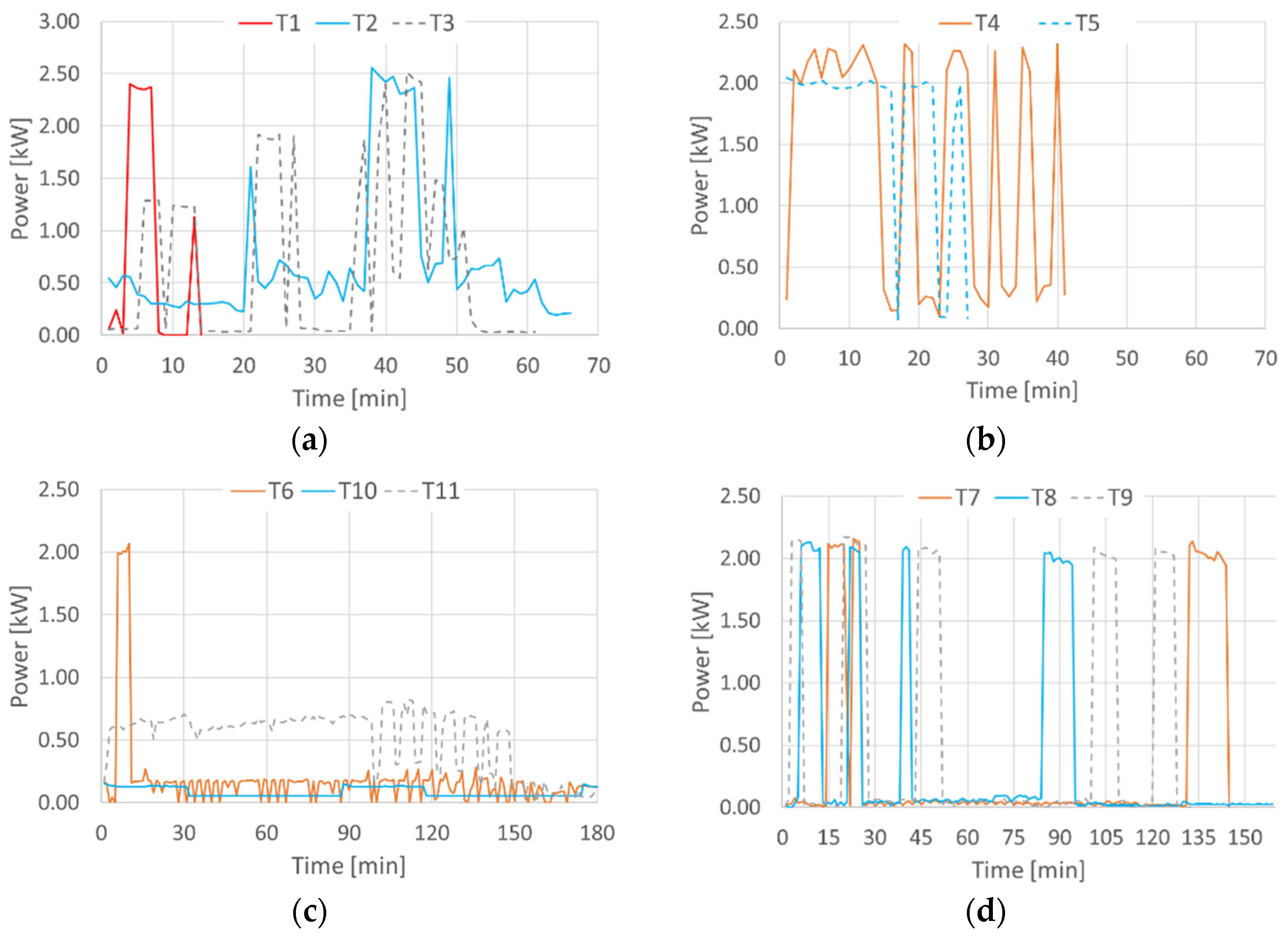
3.1. Consumption Profiles of Household Appliances

The load profiles of major household appliances were measured during the experimental analysis, described in Section 2.1. The graphs in Figure 5 show the trend over time of the electrical power consumed by different household appliances according to different operating programs. In many cases, a high peak load is noticed but only for short time intervals. This is usually related to the switching on and off of the electric resistance used to heat water in the washing machine and dishwasher or to heat the oven. Even the induction hob has medium to high peaks but limited in time. In the base load, a repetitive profile can be seen in which the power varies from a few watts to about 150 W due to the switching on of the refrigerator and freezer compressors. The impulsive nature of these loads poorly matches the instantaneous availability of PV-generated power. The only household appliance that shows a consistent draw profile over time is the heat pump dryer (T11).

The derived experimental profiles were later used in a Matlab code to develop annual load profiles considering the number of daily switch-on and probability distributions on the time of appliance activation published in [21]. All 5 clusters identified by the authors were considered. In fact, while Cluster 1 (cl.1), 2 (cl.2) and 3 (cl.3) tend to represent the families with higher consumption, cluster 6 (cl.6) and 7 (cl.7) represent the most cost (and energy)-conscious households.

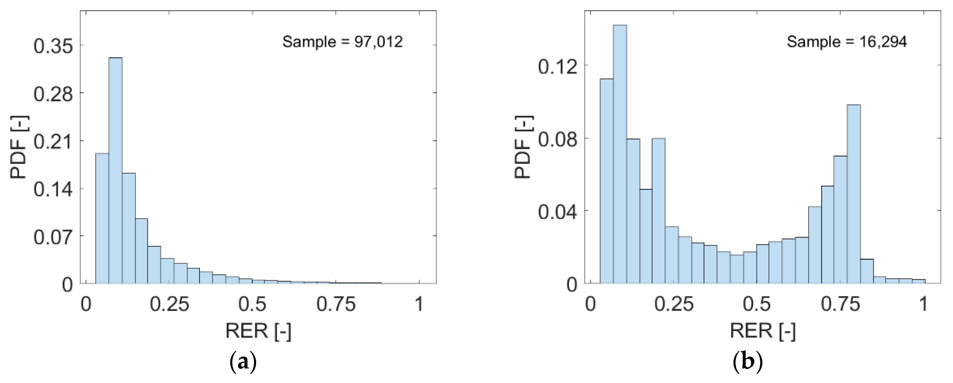
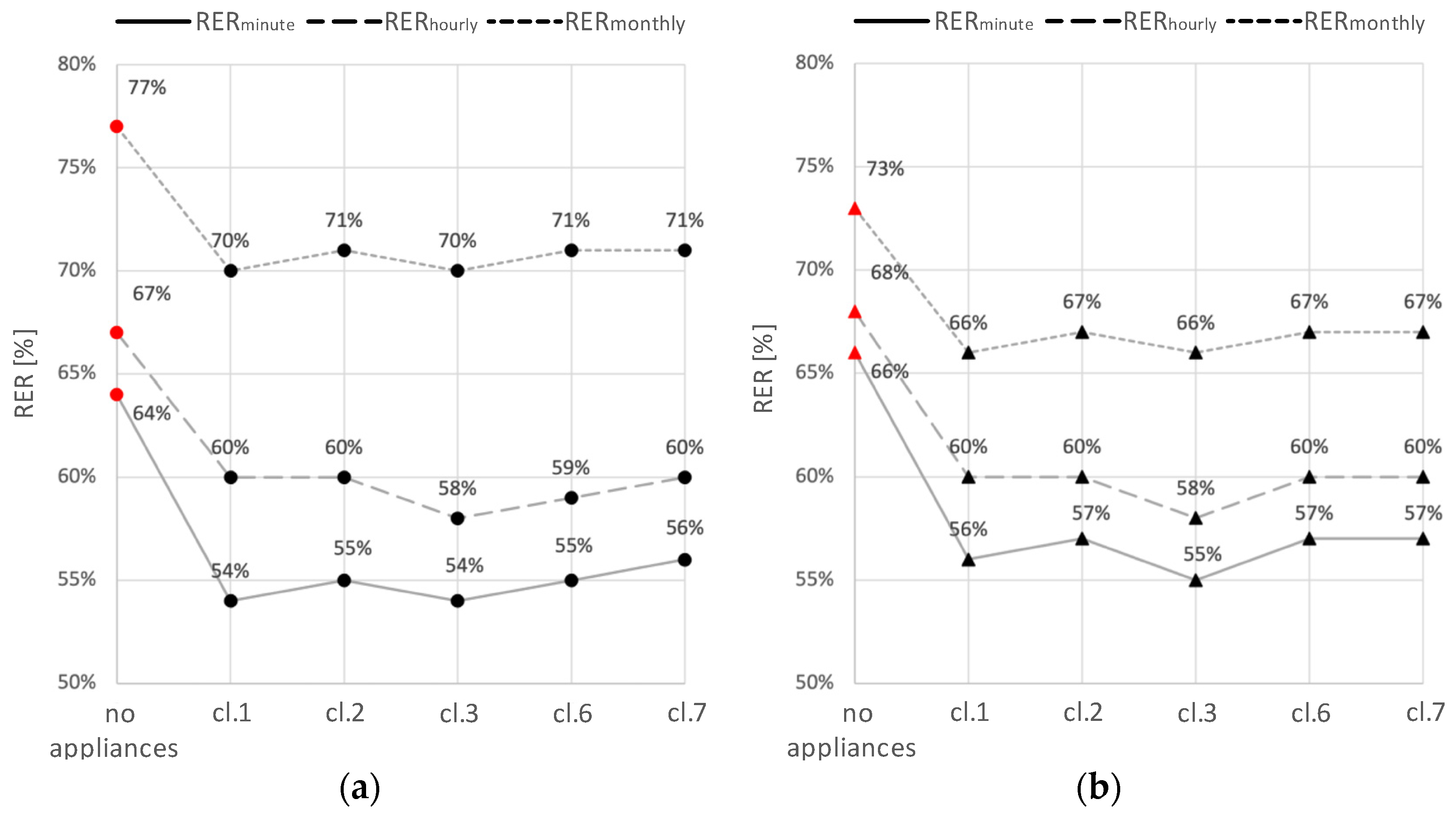
3.2. Time Base Effect on RER Index

The first results of the dynamic simulations performed highlight the extent to which the time base used in calculating the RER affects its value. For this purpose, the RER index was calculated using a time base of a minute, hour and month from simulations with basic (bas) or enhanced (enh) control of the water storage temperatures maintained by the heat pump. In the first scenario, the HP is activated to keep the temperature of the storage tanks within the variation band, while in the second control strategy, the SCF of the PV generation is maximized by overheating the storage tanks in case of available PV surplus. In both cases, the RER indices were evaluated by either considering or not the energy consumption of the household appliances.

The RER index without plug loads increases by 13% and 10%, changing the balance closure interval from a minute or an hour to a month (Figure 6a). Figure 6b shows as RER_minute and RER_hourly increase by 2% and 1% when the advanced HP control is applied and plug loads are neglected, while on the contrary, RER_monthly decreases to 4%. This result shows that, in general, an advanced control is beneficial on system operation. However, since the regulatory framework currently evaluates the energy balance with the grid on a monthly basis, it does not reward control strategies that increase the actual (instant) self-consumption of PV energy (reducing the exchange with the grid) through an increased total consumption. In fact, the rule-based control results in an increased annual consumption from 3768 kWh to 4557 kWh (Figure 7). The Italian mandatory constraint on a RER_monthly greater than 60% is easily satisfied by HP and PV even in the mountainous context of Trento. The lower performance of heat pumps as the outdoor temperature decreases results in a reduction of renewable energy taken from the outdoor air source but it is partly offset by PV production.

Another important result is related to changes in RER as a function of tb. While a noticeable variation is present between monthly and hourly time-bases, the increase between hourly and minute tb is less pronounced both with bas and enh controls. It is clear in Figure 6a,b how the presence of household appliances leads to a significant decrease in RERs. Obviously, because the total primary energy consumption increases but the monthly PV production remains unchanged. What is interesting, however, is how the RER_minute has a higher decline than the RER_monthly and RER_hourly. This is largely related to the fact that the habits highlighted in [21] show a tendency for large appliances to be used during the hours with little PV production. This, in addition to the nature of appliance loads, leads to a worsening of the index when the possibility of exploiting the exchange with the grid is lost. Nonetheless, the RER values differ by only 1% ÷ 2% among different clusters, thus highlighting a limited impact of load profiles on the index.

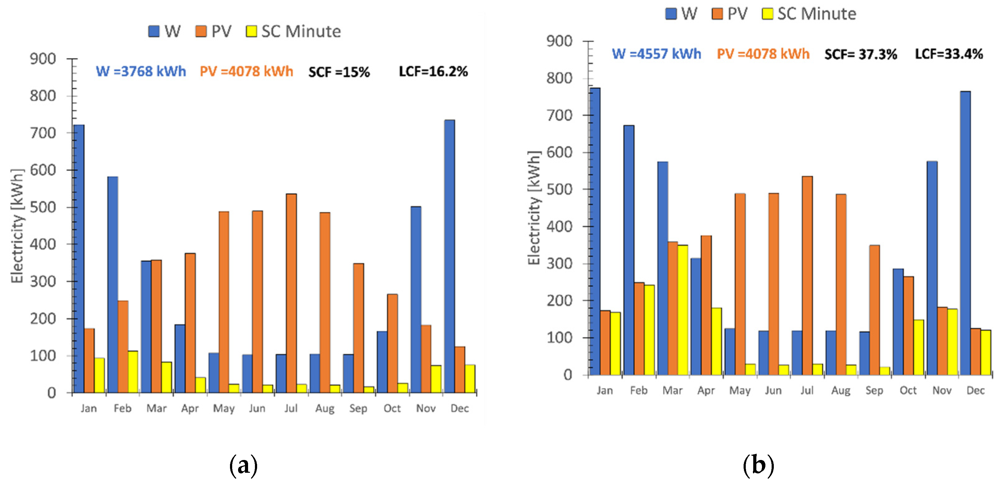
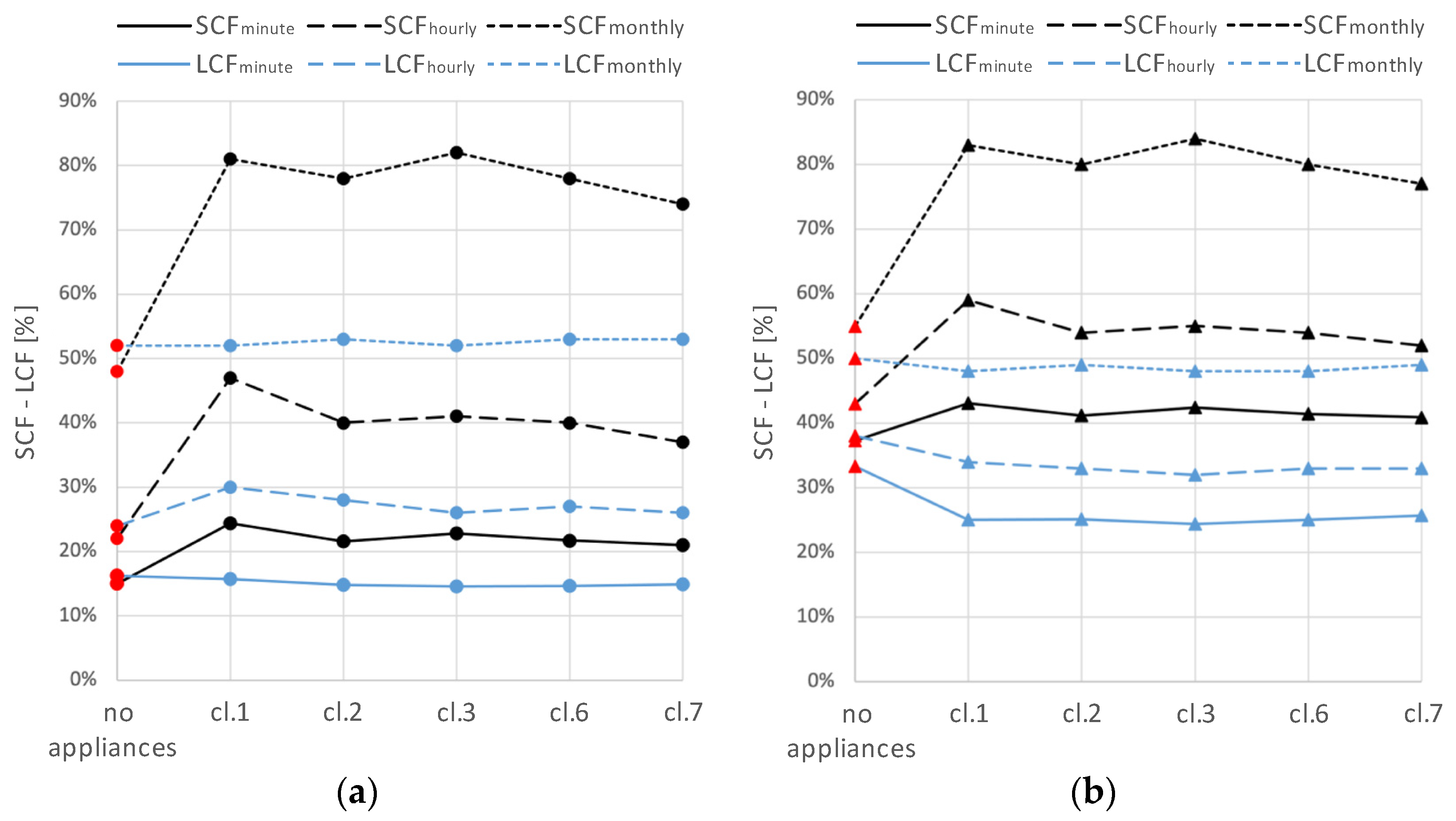
3.3. Time Base Effect on LCF and SCF Indexes

A similar analysis is performed on the self-consumption and load coverage factor. The advantage of a rule-based control becomes much more apparent by comparing the graphs in Figure 7a,b. When comparing the two charts, an increase in self-consumption can be seen, and especially in Figure 7b where the yellow bar representing self-consumption tends to the red bar of PV production in the winter months. In contrast, the absence of the building’s cooling requirements severely limits the self-consumption in the summer months. On an annual basis, however, a significant increase in both self-consumption factor and load coverage factor can be seen although enhanced control leads to an overall increase in energy consumed.

The improved coupling of PV to HP provided by the advanced control is most evident in the improvement of self-consumption (Figure 8). In fact, SCF increases by 7%, 21% and 22% in the case of monthly, hourly or minute tb, when advanced control is implemented, and appliances are not considered. LCF also varies, but in this case, while with hourly and monthly tb, advanced control leads to an increase in self-sufficiency of 14% and 17%, with monthly tb, there is a slight decrease of 2%. This is related to constraints on HP operation for which there is a minimum run time following each start and thus, higher consumption not covered by PV is possible. This constraint is set by the manufacturers to avoid continuous on/off cycles that would reduce the compressor life.

A first noticeable result when comparing the effect of appliance load profiles in Figure 8 is the limited variability (lower than 7%) of LCF and SCF between clusters. Different habits on operating hours and different equipment of household appliances do not seem to affect self-sufficiency and self-consumption remarkably. However, considering the electricity consumed by household appliances leads to a significant increase in SCF, which is obviously more pronounced in the case of a monthly net metering scheme. In this case, in fact, SCF increases between 26% and 33% in the different clusters regardless of the type of HP control. The appliances are still beneficial in improving self-consumption even in the case of hourly or per-minute tb. However, by reducing the value of tb, the control strategy adopted becomes more important. Home appliances, on the other hand, do not seem to lead to appreciable improvements in the LCF index. In fact, an LCF substantially similar to the case without appliances is noted with a standard HP control and monthly or minute tb. On the contrary, improvements between 2% and 6% are present in the LCF index when an hourly tb is adopted.

A general worsening of the LCF index is noted in Figure 8b, especially in the case of smaller tb. In fact, the advanced control acts only on the HP, and the addition of further consumption that is only to a small extent covered by PV production jeopardizes the effect of the enh control. However, the LCF indices obtained in Figure 8b are always higher than those in Figure 8a, except for monthly values.

4. Discussion

Experimental results show that the consumption of large household appliances often has high peaks lasting for short time intervals. This characteristic is not conducive to self-consumption of PV production especially when tb is limited. The same consideration can be made for the heating and DHW systems, especially when the heat pump operates following a standard strategy such as proportional controls for restoring the setpoint temperature in the buffer storage tank. For example, when the heat pump operates to heat domestic hot water, it typically tries to restore the temperature in the thermal energy storage as quickly as possible, thus working at maximum capacity. Hence, the peak power consumption will be high and time limited. This explains the non-negligible influence of tb on the RER, SCF and LCF indices. If exchanges with the grid can be balanced on a longer time interval, this leads to an improvement in the indices that quantify the renewable share.

More advanced control strategies, which aim to make more intelligent use of the availability of thermal energy storage, inevitably improve instantaneous self-consumption and consequently reduce the dependence of performance indices on the tb used, as is evident from the graph in Figure 8b. However, there remains a significant deviation if the electrical inputs of household appliances are also considered. In fact, in this case, in absence of electric batteries, it would be important for household appliances to modulate their load according to PV availability, following a demand–response logic.

5. Conclusions

The time interval base tb used to calculate renewable shares has a noticeable influence on both RER and LCF indexes. This is largely motivated by the nature of the load profiles of household appliances as shown by the experimental analysis. In fact, in the large appliances monitored, only the dryer machine has a profile that matches PV production while the other appliances have high and short duration peaks. Likewise, a standard heat pump control logic is not optimized to take advantage of PV power; hence, advanced logic may be beneficial to increase the renewable share. For these reasons, the RER calculated with a tb of one minute decreases, compared with the monthly tb, by 13% and 7%, respectively, with traditional or enhanced heat pump control. If household appliances consumption is also included in the RER, the decrease is 15% and 10% always in the case of standard or enhanced control.

Comparison between the RER index used in European standards and the LCF clearly shows how the latter is obviously lower. In analyses carried out in the absence of appliance load, the difference with monthly tb is 25% and 23% in the case of standard or advanced heat pump control, respectively. The difference increases to 48% and 33% in the case of minute tb. Since it is expected that the regulatory framework will evolve toward scenarios limiting the exchange with the national grid (e.g., introducing penalizing tariffs and/or requiring the closure of the balance within shorter time intervals), advanced control strategies will become more and more important in the future, especially in heating dominated climates.

In the harsh Alpine climate, where the orography reduces the availability of solar radiation, the heat pump is still able to achieve monthly RER values almost always above 70% in both the case with and without appliances (Figure 6). These values are close to the values achievable with a wood fired boiler but have the substantial advantage of avoiding particulate matter emissions in the atmosphere.

References

1. International Energy Agency (IEA). Tracking Buildings 2021; Tracking Report; IEA: Paris, France, 2021; Available online: https://www.iea.org/reports/tracking-buildings-2021 (accessed on 30 March 2022).
2. European Commissione (EU). EU energy in Figures—Statistical Pocketbook 2021; European Commission: Luxembourg, 2021. [Google Scholar]
3. D’Agostino, D.; Parker, D. Data on cost-optimal Nearly Zero Energy Buildings (NZEBs) across Europe. Data Brief 2018, 17, 1168–1174. [Google Scholar] [CrossRef] [PubMed]
4. REPowerEU Plan. Communication from the Commission to the European Parliament, the European Council, the Council, the European Economic and Social Committee and the Committee of the Regions: REPowerEU Plan; European Commission: Luxembourg, 2022. [Google Scholar]
5. European Parliament (EU). Renewable Energy Directive (RED II), Directive (EU) 2018/2001 of the European Parliament and of the Council of 11 December 2018 on the Promotion of the Use of Energy from Renewable Sources; European Parliament: Luxembourg, 2018. [Google Scholar]
6. Decreto Legislativo 8 Novembre 2021, n. 199. Attuazione Della Direttiva (UE) 2018/2001 del Parlamento Europeo e del Consiglio, dell’11 Dicembre 2018, Sulla Promozione Dell’uso Dell’energia da Fonti Rinnovabili; Presidente della Repubblica: Roma, Italy, 2021.
7. Luthander, R.; Widén, J.; Nilsson, D.; Palm, J. Photovoltaic self-consumption in buildings: A review. Appl. Energy 2015, 142, 80–94. [Google Scholar] [CrossRef] [Green Version]
8. Fisher, D.; Madani, H. On heat pumps in smart grids: A review. Renew. Sustain. Energy Rev. 2017, 70, 342–357. [Google Scholar] [CrossRef] [Green Version]
9. Pinamonti, M.; Prada, A.; Baggio, P. Rule-Based Control Strategy to Increase Photovoltaic Self-Consumption of a Modulating Heat Pump Using Water Storages and Building Mass Activation. Energies 2020, 13, 6282. [Google Scholar] [CrossRef]
10. Savolainen, R.; Lahdelma, R. Optimization of renewable energy for buildings with energy storages and 15-minute power balance. Energy 2022, 243, 123046. [Google Scholar] [CrossRef]
11. Amato, A.; Bilardo, M.; Fabrizio, E.; Serra, V.; Spertino, F. Energy Evaluation of a PV-Based Test Facility for Assessing Future Self-Sufficient Buildings. Energies 2021, 14, 329. [Google Scholar] [CrossRef]
12. Kotarela, F.; Kyritsis, A.; Papanikolaou, N. On the Implementation of the Nearly Zero Energy Building Concept for Jointly Acting Renewables Self-Consumers in Mediterranean Climate Conditions. Energies 2020, 13, 1032. [Google Scholar] [CrossRef] [Green Version]
13. Franzoi, N.; Prada, A.; Verones, S.; Baggio, P. Enhancing PV Self-Consumption through Energy Communities in Heating-Dominated Climates. Energies 2021, 14, 4165. [Google Scholar] [CrossRef]
14. Cirone, D.; Bruno, R.; Bevilacqua, P.; Perrella, S.; Arcuri, N. Techno-Economic Analysis of an Energy Community Based on PV and Electric Storage Systems in a Small Mountain Locality of South Italy: A Case Study. Sustainability 2022, 14, 13877. [Google Scholar] [CrossRef]
15. Musall, E.; Voss, K. Renewable Energy Ratio in Net Zero Energy Building. REHVA J. 2014, 51, 14–18. [Google Scholar]
16. Kurnitski, J. Technical definition for nearly zero energy buildings. REHVA J. 2014, 50, 22–28. [Google Scholar]
17. Tostado-Veliz, M.; Kamel, S.; Aymen, F.; Jurado, F. A novel hybrid lexicographic-IGDT methodology for robust multi-objective solution of home energy management systems. Energy 2022, 253, 124146. [Google Scholar] [CrossRef]
18. Huber, P.; Ott, M.; Friedli, M.; Rumsch, A.; Paice, A. Residential Power Traces for Five Houses: The iHomeLab RAPT Dataset. Data 2020, 5, 17. [Google Scholar] [CrossRef] [Green Version]
19. Cuerdo-Vilches, T.; Angel Navas-Martin, M.; Oteiza, I. Behavior Patterns, Energy Consumption and Comfort during COVID-19 Lockdown Related to Home Features, Socioeconomic Factors and Energy Poverty in Madrid. Sustainability 2021, 13, 5949. [Google Scholar] [CrossRef]
20. Analisi Tecnico-Economica di Interventi di Riqualificazione Energetica Del Parco Edilizio Residenziale Italiano. Available online: https://www.rse-web.it/rapporti/analisi-tecnico-economica-di-interventi-di-riqualificazione-energetica-del-parco-edilizio-residenziale-italiano-315557/ (accessed on 1 July 2022).
21. Besagni, G.; Premoli Vilà, L.; Borgarello, M. Italian Household load profiles: A monitoring campaign. Buildings 2020, 10, 217. [Google Scholar] [CrossRef]
22. EN 50470; Electricity Metering Equipment (a.c.). Comité Européen de Normalisation: Bruxelles, Belgium, 2008.
23. EN/IEC 62053; Electricity Metering Equipment—Particular Requirements. Comité Européen de Normalisation: Bruxelles, Belgium, 2020.
24. Decreto del Presidente Della Repubblica 412/93; Regolamento Recante Norme per la Progettazione, L’installazione, L’esercizio e la Manutenzione Degli Impianti Termici Degli Edifici ai Fini del Contenimento dei Consumi di Energia. Presidente della Repubblica: Roma, Italy, 1993.
25. UNI 10349-1; Riscaldamento e Raffrescamento Degli Edifici—Dati Climatici—Parte 1: Medie Mensili per la Valutazione Della Prestazione Termo-Energetica Dell’edificio e Metodi per Ripartire L’irradianza Solare Nella Frazione Diretta e Diffusa e per Calcolare L’irradianza Solare su di una Superficie Inclinata. Ente Nazionale Italiano di Unificazione: Roma, Italy, 2016.
26. Decreto del Presidente Della Provincia 13 luglio 2009, n. 11-13/Leg; Disposizioni Regolamentari in Materia di Edilizia Sostenibile in Attuazione del Titolo IV Della Legge Provinciale 4 Marzo 2008, n.1 (Pianificazione Urbanistica e Governo del Territorio). Provincia Autonoma: Trento, Italy, 2009.
27. Bee, E.; Prada, A.; Baggio, P. Variable-speed air-to-water heat pumps for residential buildings: Evaluation of the performance in northern Italian climate. In Proceedings of the 12th Rehva World Congress (CLIMA2016), Aalborg, Denmark, 22–25 May 2016. [Google Scholar]
28. UNI TS 11300-5; Prestazioni Energetiche Degli Edifici—Parte 5: Calcolo Dell’energia Primaria e Della Quota di Energia da Fonti Rinnovabili. Ente Nazionale Italiano di Unificazione: Roma, Italy, 2016.
Figure 1. Probability density function (PDF) of RER in the energy certificates of Lombardy on the left (a) and Trentino on the right (b). Only certificates with RER greater than zero were analyzed.
Energies 16 00384 g001
Figure 2. Single-family building (MF).
Energies 16 00384 g002
Figure 3. Schematic diagram of the heating system.
Energies 16 00384 g003
Figure 4. Layout of the developed TRNSYS model.
Energies 16 00384 g004
Figure 5. Measurements of electrical absorptions of the different programs of the induction hob (a), oven (b) base load, washing and dryer machines (c) and dishwasher (d).
Energies 16 00384 g005
Figure 6. Annual values of RERminute, RERhourly and RERmonthly: TRNSYS results for the MF building in Trento, without (red) and with appliances (black) and bas (a) or enh (b) controls.
Energies 16 00384 g006
Figure 7. Monthly trends in W, PV and self-consumption in the no appliance case with standard control (a) and with rule-based control (b).
Energies 16 00384 g007
Figure 8. SCF and LCF factor, without (red) and with appliances (black) and bas (a) or enh (b) controls.
Energies 16 00384 g008