Estimation of Vehicle Energy Consumption at Intersections Using Microscopic Traffic Models

Abstract

This paper addresses issues related to modeling energy consumption and emissions using microscopic traffic simulations. This paper develops a method in which a traffic model is used to calculate the energy needed to travel through selected types of intersections. This paper focuses on energy consumption and derived values of calculated energy, which can be, for example, carbon dioxide emissions. The authors present a review of the scientific literature on the study of factors affecting energy consumption and emissions and methods to estimate them in traffic. The authors implemented an energy consumption model into a microsimulation software module to estimate results as a function of varying traffic volumes at selected types of intersections and for selected traffic organization scenarios. The results of the study show the lowest energy consumption and the lowest emissions when road solutions are selected that contribute to reducing vehicle travel times on the urban street network at higher average vehicle speeds. In addition, the positive impact of the share of electric vehicles in the traffic flow on the reduction of energy consumption and emissivity was estimated.

1. Introduction

Year after year, increasing emphasis is placed on reducing greenhouse gas emissions and climate change. Transportation is responsible for part of the pollution generated, so various measures are being taken to reduce its negative impact on the environment. The right action is to modify the existing elements of the transport system and the behavior of travelers, to provide solutions that seek to reduce the emissions of harmful substances without significant deterioration in the population’s quality of life. There is a reduction in the quality of life of residents in urban centers, where the population is large, traffic congestion is frequent, and the high volume of vehicles results in high emissions of emissions and noise.

Urban transportation systems are facing serious challenges due to the increase in motorization rates (the number of private vehicles per population) and the number of private vehicles [1,2]. More than 256 million passenger cars were in the European Union (EU) countries in 2018 [3]. Furthermore, the World Bank forecasts show that by 2050 the number of vehicles worldwide will double to two billion, and 70% of the projected world population will live in urban areas, tripling the number of urban trips [4,5]. According to recent estimates, passenger transportation (in kilometers) in countries of the European Union will increase by 42% by 2050 [6]. In the United States, this value will increase by 30–50% by 2100 [7]. It is possible to estimate the energy needed for the operation of various modes of transportation. Vehicles on the road, especially passenger cars, considering the MJ/passenger-km indicator, consume the most energy, reaching values of 4.7 and 4.4 for diesel and petrol cars, respectively. At the same time, buses obtain a value of 2.8, while bicycles achieve a value of 0.8 MJ/passenger-km [8].

Many cities around the world are experiencing urban sprawl, resulting in rapidly increasing motorization and a high share of automobile travel, often inadequate and inefficient public transportation systems, poor infrastructure for active mobility (pedestrians and cyclists), and high environmental pollution [9].

The unsustainable growth of transportation activity is putting a strain on the ecosystems and resources of the planet. Greenhouse gas (GHG) emissions from energy production are one of the main causes of climate change. In Europe, greenhouse gases decreased between 1990 and 2017, except for the transportation sector [10]. The transportation sector represents 30% of total energy consumption and 20% of total GHG in the European Union (with road transport accounting for the largest share at 72%) [10,11,12]. Although new and increasingly restrictive emission standards have been emerging over the years and are evident in the declining emissions of newly manufactured cars [13], a similar share of carbon dioxide production by road transport has been maintained over the years [8].

The slow transition to propulsion systems and alternative fuel sources has caused the transportation sector to be increasingly blamed for the possible failure of individual countries to meet their commitments to international climate change agreements [9]. For this reason, transportation is still at the center of any debate on energy conservation, due to its reliance on fossil fuels for, among other things, automobile transportation (freight and passenger).

In 2019, the European Commission revised its earlier calculations of the environmental and social impacts of transportation. The total external environmental costs of transportation (related to climate change, air pollution, noise, well-to-tank, and habitat damage), accident costs, and congestion add up to €987 billion annually in the EU. This includes the environmental costs of approximately €434 billion, road accident costs estimated at €286 billion, and congestion costs of €267 billion. The urban share is estimated to be at least 50%. Road transportation causes more than 80% of such external costs (approximately €620 billion caused by passenger transport and €200 billion by freight) [14]. This is a very significant increase over the calculations in the 2013 transportation impact assessment, where the total external costs of transportation were estimated at €420 billion per year, with the urban share estimated at €230 billion [15].

There are increasing indications that electrification in transportation will not be fast enough or sufficient to achieve the low-carbon goals and energy efficiency of the transportation system [12,16,17,18]. Trends in transportation development call for measures to reduce energy consumption and increase decarbonization. Evaluating the effectiveness of such measures is possible by using transportation models that allow one to estimate energy consumption and emissions.

The municipal authorities are trying to improve the situation by investing in the development of public transport through the development of the available transport offer and the use of dedicated solutions, such as bus lanes and traffic signal priorities, aimed at encouraging travelers to use modes such as buses and trams. In addition, to reduce emissions locally, additional privileges are given to electric vehicles, such as, in Poland, the ability to enter bus lanes or free parking in designated zones. At the same time, access to urban centers is restricted by law for vehicles that do not meet established environmental standards or for motorized vehicles, in general. Furthermore, in terms of infrastructure, solutions that limit car use are applied, for example, reducing the number of lanes on wide arterials or converting existing general traffic lanes into bus lanes. In addition, solutions are introduced to ensure priority for active mobility participants: cyclists and pedestrians. For example, by building sections with shared traffic, where vehicle speeds are adjusted to accommodate walking pedestrians [19]. Rarely, however, do city authorities implement solutions that they carefully evaluate in advance for emissions that negatively affect residents’ health or climate change. The effective development of the transportation system requires predicting the effectiveness of planned changes and checking the effectiveness of the implemented measures. Most often, cities do not use tools to consider the impact of the solutions introduced in the transportation system on the health of residents and climate change as a result of the implementation of infrastructure or organizational measures. Transportation demand and transportation network models can effectively support the mobility planning process by including estimates of harmful emissions.

The purpose of this article is to study the possibility of developing a model that can support the process of evaluating the impact of selected measures of traffic organization and the type of intersections on energy consumption and carbon dioxide emissions. Due to the possibility of reproducing the actual behavior of drivers to a considerable extent, it was decided to develop a microscopic model. This article focuses primarily on calculating the value of energy and carbon dioxide (CO₂) emissions.

These days, analyses of the selection of the most effective measures to improve road infrastructure elements and traffic organization usually consider criteria of capacity, traffic conditions, and traffic safety. The criteria for selecting the type of intersection are based on the functions of the intersecting roads and traffic volumes. The evaluation of energy consumption and emissions can complement the selection of the best traffic organization scenario.

This paper presents a proposed methodology for evaluating traffic organization measures planned for introduction, considering energy consumption and emissions. These criteria can provide additional support in the decision-making process of selecting the type of intersection and traffic organization measures. This paper presents emission estimation methods available in software packages used for travel modeling and traffic forecasting in the Pomeranian Voivodeship. The packages presented later in the paper allowed for the development of a multilevel transportation system model, used in operational traffic management and planning work, and research work [20,21,22,23].

Electric vehicles are increasingly appearing in traffic. The question arises whether the share of electric vehicles in the vehicle fleet will affect the additional evaluation criteria studied in this article.

The structure of the article is planned as follows. Section 2 describes an overview of the research on factors affecting energy consumption and emissions and the methods for estimating these variables. Section 3 presents the methodology for conducting the research, including a preview of the assumptions for the research conducted, a description of the field research and its verification, and a description of the process of developing simulation models and their calibration, as well as scenarios for changes in infrastructure measures and transportation demand. The results of studies conducted using simulation models considering the adopted scenarios for the choice of intersection type and traffic organization used are presented in Section 4. A discussion of the results obtained in comparison with other studies in the area is presented in Section 5. Conclusions are presented in Section 6.

2. Methods for Estimating Energy Consumption and Emissions in Traffic: A Review

The implementation of transportation system management measures, including traffic organization and control, requires an analysis of their impact on the elements of the transportation system and the surrounding area. Assessments of the impact of planned measures on the state of the transportation system aim to verify the possibility of sustainable development of urban and rural areas in economic, social, and environmental terms. The analyses of energy consumption, air pollutant emissions, and greenhouse gas emissions should be one of the most widely used indicators for assessing the sustainability of transportation. From the point of view of assessing the environmental impact of road transport, the selection of such indicators allows us to consider its most important characteristics and associated negative impacts. This review presents the factors affecting energy consumption and the methods used to calculate energy consumption and exhaust emissions, including greenhouse gases.

2.1. Factors affecting Energy Consumption and Emissions

Emissions (including carbon dioxide) can be related to fuel consumption [24,25,26]. Energy consumption, on the other hand, is related to a wide variety of factors due to the surroundings [24,27], the static and dynamic characteristics of the vehicle [28,29], and human factors [30], which often affect the dynamic characteristics.

Some characteristics of vehicles that affect energy consumption and emissions remain constant within a given area of analysis. Among these characteristics, some never change. These are primarily the type of propulsion and fuel [25], and engine capacity [29]. Additionally, certain features can change, such as added weight (more passengers, more cargo) [24] and the front area of the vehicle (increases if additional items are carried on the roof of the vehicle) [24,28,29]. The mentioned characteristics do not change in the time interval adopted for the research [25]. Engine capacity is usually associated with a constant value of fuel consumption and emissions, regardless of operation [29].

The additional weight may change between journeys, but within a single section it is usually constant, so it can be considered a feature that remains unchanged, at least for individual vehicles within a microscopic simulation. An increase in weight results in greater resistance to movement, so the engine requires greater power to keep the vehicle moving [28,29]. Therefore, this constant element is related to the vehicle’s dynamic characteristics. In addition, according to Nouri and Morency [24], when the weight of the vehicle was increased by an added 100 kg and then 200 kg, it was observed that for the same distance of 14.5 km, emissions increased by 16.15 g and 32.31 g, respectively. In this case and the narrow scope of this analysis, a linear relationship can be seen between increasing vehicle weight and increasing CO₂ emissions. The surface area of the front end of the vehicle, as well as the curb weight, is an element that will remain constant for a given vehicle within the analysis and will also affect resistance to movement [28,29] and therefore the value of energy consumption and emissions.

The vehicle dynamic characteristics affecting instantaneous energy consumption and emissions are primarily the values of speed and acceleration [28,29,31]. Energy consumption increases the most at high acceleration values. At zero acceleration and constant speed, the value of energy consumption is constant, but as the speed increases the higher the energy consumption, which is due to increasing resistance to movement (air resistance increases with the square of speed). High energy consumption can also be observed at low speeds [24,32], which may be due to the high initial force needed to set the vehicle in motion. The described values for the dynamic characteristics are related to the weight and frontal area of the vehicle [29,33]. However, the values of speed and acceleration achieved at any given time depend on the human driving and the way the vehicle in question is driven, as well as the surroundings in which it finds itself. Another aspect related to traffic dynamics and the way the vehicle is driven is the choice of the proper gear in the vehicle. Depending on the speed, drivers change gears (or this happens automatically) [32], while individual gears allow the expected values of speed and acceleration to be achieved, so this is another element that depends on the driver.

Energy consumption and emissions are influenced by infrastructure solutions [30,34,35], applied traffic organization [34], and temporary weather conditions [26,27,36] for the factor of surroundings. In addition, the environment can include Intelligent Transportation Systems services [37]. For infrastructure, different emission values are calculated for different types of intersections [35] or depending on the number of lanes [34]. Traffic organization related to solutions such as dedicated bus lanes or different structures of traffic signal programs can change energy consumption and emissions [34]. When weather conditions change (e.g., rain or snowfall), traffic parameters on the road also change, speeds decrease, headways between vehicles increase, and capacity is reduced, which can affect queue formation or lengthening [27,36]. This contributes to changes in vehicle dynamics, which can result in different levels of energy consumption and emissions. In addition, air temperature affects engine temperature. This is an aspect related to the vehicle [26]. When the engine is warmed up, that is, in a state of thermal stability, fewer harmful substances are emitted. Even at a high ambient temperature, it takes time for the engine to warm to the target temperature, but the lower the air temperature, the longer it takes. Intelligent Transportation Systems services, such as traffic control or directing vehicles to alternative routes, help improve traffic conditions. These are just some of the elements of the overall system that contribute to improving traffic conditions in the transportation network while reducing energy consumption and emissions.

A complement to the factors described above is the human being in charge of driving. They are the one who selects the speed, behaves in different ways depending on the situation and weather conditions, and reacts in various ways to the measures on the road and the traffic conditions [30,36,38]. There are separate ways to classify driver behavior, but the general idea is to set up a distinction between gentle and aggressive driving styles. The main observation within this classification is the increase in fuel consumption and emissions within the more aggressive style [39,40,41,42,43]. Different criteria can be applied, but usually, acceleration and speeds higher than average for a set number of observations are the main distinguishing factors. An additional measure can be counting the number of times the gears were changed [44]. Driver behavior may vary according to the environment or even the country where the investigation is performed [45].

2.2. Methods for Estimating Energy Consumption and Emissions

Depending on the purpose of the study and its details, traffic models in the transportation network consider micro-, meso-, or macroscopic relationships. Macroscopic and mesoscopic models make it possible to estimate typical measures of transportation system efficiency (e.g., vehicle kilometers traveled and total vehicle travel time on the transportation network). Macroscopic models consider the capacity of various types of roads, the speeds of vehicles in free-flow traffic, and the resistance functions for different sections of the road network. Mesoscopic models also consider the impact of traffic organization and control, which decide the formation of queues for vehicles and delays within intersections. Mesoscopic models define traffic characteristics and network elements at a higher level of detail than macroscopic models by considering the interrelationships between traffic characteristics at critical locations and their influence on driver behavior about the choice of lanes or travel routes. In the microscopic approach, each vehicle in the network is simulated continuously at the individual level, considering the driver’s response to external stimuli (e.g., caused by traffic signals or information provided by road signs) and considering changes in speed, stopping, and traffic trajectories in interaction with other road users [20,21,22,23].

Two typical approaches to calculating energy consumption and emissions can be distinguished [33,46]:

• Fleet-based—which involves calculating energy consumption and emissions values with knowledge of the number and type of structure of vehicles and the distance they traveled, often including additional variables such as average speed;
• Instantaneous—which involves calculating instantaneous emissions or instantaneous energy consumption based on the simulation of each vehicle individually, taking into account the instantaneous variables describing a specific vehicle, often used to simulate a smaller number of vehicles, but with greater accuracy.

The fleet approach can be applied to macroscopic and mesoscopic methods for estimating energy consumption and exhaust emissions, while the instantaneous approach is most often used in microscopic methods.

2.2.1. Macroscopic Approach

The PTV VISUM software allows the use of basic procedures to calculate energy consumption and estimate the environmental impact of transportation-related noise and pollution emissions. For emissions calculations, the basic procedure is Pollution-Emis. Polynomial regression curves up to the fifth degree were used to calculate emissions along sections of the road network, considering the speed of passenger vehicles and trucks and the volume of traffic along a section of the road network [47].

HBEFA (Handbook Emission Factors for Road Transport) [48] presents current emission factors for all vehicle categories. To find the level of air pollution caused by emissions and to evaluate measures to reduce pollution, data on specific types of emissions must be collected for each vehicle category. For this purpose, the environmental agencies in Germany (UBA), Austria (UBA), and Switzerland (BAFU) have been supporting these studies for many years, the results of which are presented in successive HBEFA updates. The calculations performed in the PTV VISUM software consider variables that characterize traffic conditions, traffic volume, and vehicle fleet structure (by country, year, and category) in sections of the road network (excluding intersections). Emissions are calculated depending on the available data and the structure of the travel model. For hot engine emissions calculations, the longitudinal gradient of the road and its type (e.g., urban, suburban, highway) can be considered. The division of the demand segment into the cold start and hot engine vehicles is carried out by considering the origin zone of the trip and analyzing the travel time and length of the routes taken by vehicles of each category. Examples of the use of PTV VISUM software to estimate emissions were presented by Ambroziak et al. [49] and Jacyna et al. [50].

2.2.2. Mesoscopic Approach

The SATURN software [51] allows fuel consumption and emissions estimation based on user-specified procedures using characteristics calculated with a traffic model of the transportation network and exogenous data (e.g., weather conditions) that can be input into the SATURN package’s database. Regardless of the ability to develop custom emission estimation models, SATURN includes internal procedures for calculating the emissions of carbon monoxide and dioxide, hydrocarbons, nitrogen oxides, and PM 10. The methods use linear models with explanatory variables including travel time (speed), trip length, and the number of stops at individual sections in the road network model. The default values for the coefficients of the equations for each type of emission were taken from the paper by Matzoros and van Vliet [52]. Due to the lack of up-to-date data, estimating emissions requires using the author’s procedures or updating the coefficients and adapting them to current conditions. Using the default coefficients, the internal model in the SATURN software only allows a comparison of the scale of the impact of making changes to the transportation network model or travel model on pollutant emissions.

2.2.3. Microscopic Approach

The PTV VISSIM software allows for the calculation of air pollutant emissions using three procedures [53]. The first is a simplified method for estimating emissions within a user-marked area known as a node. The procedure assumes the use of equations to calculate fuel consumption and emissions, as proposed in the TRANSYT 7-F method based on Oak Ridge National Laboratory research [54]. The computational model uses data on engine operation in terms of the distance traveled during acceleration from initial to target speed, driving at a constant speed, and stopping while braking, considering the longitudinal gradient of the roadway [54].

The second available method assumes the use of the external EnViVer software, which allows estimating emissions from detailed vehicle trajectory data extracted from simulations in VISSIM in terms of vehicle speed profiles considering the longitudinal gradient of the road section and the type of vehicle. There are default emission classes in the software for selected types of vehicles, considering urban, rural, or highway roads, as well as the share of cold start vehicles. Calculations consider the introduction of regulations following the European emission standard (Euro 1–6), the age structure of vehicles, and the type of fuel used (gasoline, diesel, LPG, CNG, electric vehicle). The software makes it possible to calculate exhaust emissions using the VERSIT+ model [55,56] and to visualize estimates of exhaust gas dispersion depending on the road environment (e.g., open terrain, one-sided or two-sided buildings along the road).

The third way to estimate emissions is to use external user libraries and the emission models implemented in them. Basic data that can be extracted from the PTV VISSIM traffic model for individual vehicles and the simulation time step are acceleration, speed, number of stops, queuing time, ID, vehicle type, and longitudinal gradient of the road. Baseline data and other simulation data can be used to develop external emission models, for example, the model developed by Stevanovic et al. [57]. Furthermore, the simulation provides the ability to consider several types of drivers, depending on driving dynamics. Microscopic models oftentimes require calibration that tailors simulated driver behavior following real-life situations. There are different ways to approach this issue. Essential values such as queue length can be recorded and then reproduced. More complex ideas consist of recording the driver trajectory (e.g., using a smartphone) and then extracting these data to receive precise measures [58].

The third method described has been used to conduct the research presented in this article in estimating energy consumption and carbon dioxide emitted. The equations for energy consumption were developed in the form of an algorithm and implemented into a simulation model.

3. Materials and Methods

The methodology for conducting the study is described below, and the results and verification of field measurements are presented, which were used by the authors of the article to develop and calibrate the model. In addition, the process of developing and calibrating the model and the variables used in the process is described in the paper. The method used made it possible to estimate the value of energy consumption and the value of emitted exhaust gases under various scenarios of changes in transportation demand and intersection modernization and changes in traffic organization at the sample intersection. It is necessary to create a universal model to compare the results of the study to evaluate the impact of traffic organization and the type of intersection on minimizing vehicle movement resistance. It is impossible to find a single intersection where different traffic organization and control strategies are in place, and traffic volumes at the time of measurement reach values only within a certain closed range. By using a tool to develop microscopic traffic simulations, it is possible to supply comparable traffic conditions and volumes when analyzing different solutions and to study potential changes in vehicle volumes and directional structure.

A diagram of the research conducted, describing the evaluation method, is shown in Figure 1. The first stage of the research was the designation of a test site, which was used to collect actual traffic data. Measurements and observations were then recorded, including traffic volume, queue lengths, the distance between vehicles, and the general behavior of drivers waiting to join traffic at minor turns at the intersection. A microscopic traffic model was then developed to simulate the test site. The parameters of driver behavior were changed to converge with the recorded data in the iterative process. Once the results of the initial model were satisfactory, an energy consumption model was prepared as an external module for use in the simulation. The next steps were to prepare individual scenarios for traffic organization and intersection type for testing with the traffic measurements taken. Finally, scenarios for different traffic volumes were developed and evaluated against the aforementioned scenarios related to the road solution. The entire process allowed us to obtain energy consumption results for a wide range of scenarios while achieving a satisfactory level of reliability due to the initial calibration of the model. The detailed process to obtain results in the individual steps of the method is presented in Section 3.1, Section 3.2, Section 3.3, Section 3.4 and Section 3.5.

3.1. Study Object and Field Measurements

The first step of the research was for the authors of the article to find a potential testing ground. These basic criteria used to select an intersection for analysis were adopted:

• Traffic at the intersection is marginally affected by the impact of nearby intersections;
• The layout of the intersection allows the traffic organization to be changed to one that could exist in reality;
• Traffic conditions at the intersection are saturated due to the relatively high volume, but there is no congestion leading to paralysis of the entire surrounding road network.

The object under investigation is at the intersection of Dąbka Street and Zielona Street, in the city of Gdynia, in the Pomeranian Voivodeship, in Poland. The location of the intersection is marked in Figure 2. In its current state, the intersection is equipped with traffic signals with a signal cycle time of 60 s. Additionally, at the intersection at night and in the morning, and in exceptional situations, traffic signals are turned off and the following traffic organization is in effect: priority along Zielona Street (northern and southern entries), STOP signs on Dąbka Street (eastern and western entries). The distance from nearby intersections is 400 to 600 m at the eastern, southern, and western entries and 2500 m at the northern entry. There are no traffic disruptions at nearby intersections that would lead to the formation of such long queues so as to affect traffic at the Dąbka–Zielona intersection. Given the traffic conditions and existing organization, the chosen location favors the research of introducing alternatives for the type of intersection and traffic organization.

The traffic field measurement was performed after choosing the testing site. The main goal was to record values that would later be reproduced in a microscopic model. The behavior of drivers, in particular their approach to making a left turn, was observed. On the eastern entry, the drivers waiting to perform this maneuver were blocking the remaining vehicles in the queue. On the western entry, the drivers usually placed themselves to the very left or to the very right, creating two artificial lanes, while in reality there is only one lane on each entry. This allowed efficient passing through the intersection, even if multiple vehicles were waiting to turn left. On the remaining entries, the behavior of drivers was more usual, but a single vehicle waiting for maneuvers usually did not block the remaining vehicles waiting in the queue. The number of vehicles queuing at red signals and landmarks near the end of the queue was observed. This allowed for additional verification, as these points of interest (e.g., individual buildings) were later identified with the use of satellite imagery. The number of vehicles waiting to cross the intersection, along with additional information on the location of the last vehicle observed, served as an additional check to obtain model convergence. The purpose of the study was to simulate driver behavior and traffic characteristics to study the scenarios presented in the article, rather than testing only the existing intersection. Therefore, the specific values of the traffic volume were not as important as the other aspects mentioned earlier, but nevertheless influenced the traffic conditions and the behavior of the driver. This was the reason why simulations of transportation demand growth scenarios were included in the research method. However, the authors decided to perform the measurements at a relatively representative time, mid-week during rush hour. They were carried out on Thursday, 1 September 2022, at the most heavily trafficked hour at this location, i.e., 15:00–16:00 using the manual recording of traffic volumes on a measurement sheet. The measurements were carried out in a team of two, due to the existing signaling program (the green light is simultaneously displayed on two opposing entries, i.e., vehicles from either the N and S or E and W entries drive simultaneously) and each member of the survey team was responsible for surveying two adjacent entries: N and E or S and W, so vehicles driving from a single entry were counted at a time, which could help minimize the measurement error. The technique used allowed the intersection to be represented in a microscopic simulation, so full measurements were not repeated. Queue length, especially for the mentioned landmarks, and driver behavior were observed over short periods of time on many consecutive days and remained close to the levels initially observed.

3.2. Microscopic Simulation Model Development and Calibration

The next step was to develop a model in the software used to perform microscopic traffic simulations. For this work, PTV Vissim 2022 software was used. The road network and traffic organization at the intersection were modeled using backgrounds obtained from the platform [59], which provides high-quality satellite images. The layout of the intersection under study is shown in Figure 3. The intersection geometry, traffic organization, and traffic signal programs were reproduced using previous observations and measurements. The gradient of the road was not considered. Dynamic traffic distribution in PTV Vissim software was used, which allows traffic to be distributed over the network using a matrix, where the values are the traffic volumes going from the source to the destination at a given time interval. Volumes in the model were entered at 15-min intervals. The matrices resulting from the measurements can be found in Figure 4.

The measured traffic volumes were usually the highest on the eastern entry, resulting in the longest queue. Despite the relatively high values at the northern entry, most of the vehicles turned right. Existing traffic signals allowed drivers to perform this maneuver during the red light for this entry (conditional right-turn). Therefore, the queues observed at this entry were relatively small, ranging from 1 to 2 vehicles on average. For the remaining entries, the volumes and the corresponding queues were smaller, also reaching an average value between 1 and 2 vehicles. The total volume at the intersection studied ranged from 252 to 335 vehicles per 15-min interval. Per entry, this value was between 41 and 104 vehicles. Taking into account only single relations, 1 car was the smallest amount observed, while the biggest was 78. For vehicles turning left, the heaviest trafficked entry was also the one with the longest queue, i.e., the eastern entry. That volume varied from 16 to 28 vehicles.

In the next step, the model was calibrated to reproduce the reality in a way that meaningful results could be obtained. The traffic simulation procedure used the Wiedemann 74 model, which is recommended for use in urban traffic conditions [60,61]. Each vehicle in the simulation moves at a given speed unless there is some disturbance. This disturbance usually means the presence of another vehicle on the road. Given that in a road network, many vehicles are active at the same time, models are needed to describe the interactions between these vehicles. In the case of this research, this is the previously mentioned Wiedemann 74 car-following model, in which a vehicle tries to reach a distance d from the vehicle ahead of it (the leader), and this distance is calculated from Equation (1):

d = ax + bx

(1)

ax—average standstill distance, the base value for the average desired distance between two stationary cars, with a tolerance between −1.0 m to +1.0 m normally distributed around 0.0 m and a standard deviation of 0.3 m;

bx can be described as in Equation (2):

bx = (bx_add + bx_mult × z) × √v

(2)

z—the value of range [0, 1] normally distributed around 0.5 with a standard deviation of 0.15 [61];

v—vehicle speed (m/s);

bx_add—additive part of the safety distance, the part of bx value used to adjust the time requirement values;

bx_mult—multiplicative part of safety distance, the part of bx value used to adjust the time requirement values, where a higher value equals a greater distribution (standard deviation) of safety distance.

An additional setting called slow recovery was activated, and the following variables were set:

• Speed—threshold percentage value of the expected vehicle speed. If the vehicle’s speed falls below this threshold, slow recovery is activated for this particular vehicle;
• Acceleration—percentage value of the expected acceleration value. If slow recovery is activated for a vehicle, then its acceleration is set following this parameter (it is lowered to the set percentage value);
• Distance—percentage value of the aforementioned distance between vehicles d. If slow recovery is activated for a vehicle, then its desired distance is set following this parameter (it is increased to the set percentage value).

The model of the network was filled with vehicles before the actual simulation time (15:00–16:00) so that when the results were collected, the first vehicles did not appear in the empty network. In the next iterations, the aforementioned variables of the model were changed, so that the final convergence was obtained. The calibration of the model resulted in the variables shown in

Table 1. Driver behavior variables in the microscopic model.

Category	Parameter	Value
Wiedemann 74 model variables	Average standstill distance	2.00 m
	Additive part of a safety distance	2.90
	Multiplicative part of a safety distance	3.00
Behavior during recovery from speed breakdown (slow recovery activated)	Speed	55.0%
	Acceleration	55.0%
	Distance	110.0%

.

The adoption of the variables shown in Table 1 made it possible to achieve a traffic situation that reproduced the actual situation at the intersection. In addition to the parameters mentioned above, obtained through an iterative process during calibration, the other parameters were set according to the existing values for the car-following model implemented in the PTV Vissim software. The desired vehicle speed was set in the range of 48 km/h to 58 km/h. Acceleration ranges from 1.96 m/s² to 3.5 m/s² for a starting vehicle. Once 50 km/h is reached, the range changes to 0.92 m/s² and 3.27 m/s². For deceleration, the range is from −8.50 m/s² to −6.50 m/s² when stopping the vehicle and for a speed of 50 km/h, it changes to −8.00 m/s² and −6.00 m/s². Since the study area consists of single-lane roads, typical lane changes do not occur, so the parameters associated with this maneuver remain unchanged.

3.3. Model Verification

The criterion used to assess convergence was a comparison of observed and model queue lengths. The average queues in each quarter of the measurements were recorded. For the east entry during the period between 15:30 and 16:00, the queue length increased steadily and reached a maximum during the last quarter, after 15:45. After this peak, the queue continued to slowly shorten, and around 16:00 the queue almost disappeared. In total, 955 vehicles crossed the intersection during measurement. For calculation of the average queue, each vehicle was estimated to be approximately 5 m long (including the length of the vehicle and the distance between the cars waiting in the queue). The results are shown in

Table 2. Comparison of observed queue length with modeled values.

Time	Intersection Entry	Avg. Queue (Vehicles)	Avg. Queue (m)	Avg. Queue in the Model (m)	MAE Avg. Queue (m)	MAPE Avg. Queue (%)
15:00–15:15	N	1	5	3.87	1.13	22.60
	E	4	20	20.36	0.36	1.80
	S	1	5	5.36	0.36	7.20
	W	2	10	10.90	0.9	9.00
15:15–15:30	N	1	5	4.23	0.77	15.31
	E	3	15	15.21	0.21	1.42
	S	2	10	6.85	3.15	31.54
	W	1	5	5.94	0.94	18.76
15:30–15:45	N	2	10	10.19	0.19	1.90
	E	6	30	32.24	2.24	7.47
	S	2	10	12.81	2.81	28.10
	W	2	10	6.59	3.41	34.10
15:45–16:00	N	1	5	1.58	3.42	68.40
	E	11	55	57.64	2.64	4.80
	S	2	10	7.88	2.88	21.20
	W	2	10	10.35	0.35	3.50

.

Based on the results presented, MAE, RMSE, and MAPE were calculated for the entire period and all intersection entries, obtaining values of 1.41 m, 1.83 m, and 13.8%, respectively. Considering that the measured value was recorded in the number of vehicles and that each vehicle occupied a space equal to 5.0 m in length, the results obtained are satisfactory. In addition, the verification was considered satisfactory because the developed model is used for comparative studies within the defined scenarios. The highest error values were obtained for entries with the shortest queues, especially when the traffic volume at a given entry was exceptionally low, resulting in almost no queues. The second-highest error values were obtained for entries where the queue in the model was somewhere in the middle of the 5-m increment. Due to the method used to calculate queues (the number of vehicles in the queue), it was not possible to record values with an increment of 0.5 vehicles. Given that the worst traffic conditions were observed on the eastern entry of the intersection, achieving high convergence on this entry was the most important part of the calibration, and the results compensate for the slightly higher errors obtained for entries where traffic conditions were good, both in the developed model and during field measurements.

3.4. Estimation of Fuel and Energy Consumption and Carbon Dioxide Emission

Once the model calibration was completed, it was necessary to prepare the following elements in the research method:

• A model that calculates the energy consumption that is usable during the simulation process;
• Scenarios for changing traffic organization at the intersection;
• Scenarios for changing traffic volumes at the intersection.

The basis for calculating emissions, in particular carbon dioxide consumption, is the amount of fuel consumed, while fuel consumption and energy consumption are usually calculated based on the resistance to vehicle movement that a vehicle must overcome. For this reason, it was decided to study primarily the size of the forces responsible for resistance to vehicle movement. The primary aim of this article is to study the impact of a road solution on the energy cost needed to drive through a given intersection under certain traffic conditions. For this reason, it was decided to study resistance to vehicle movement. In this approach, achieving lower values for the resistance to vehicle movement results in lower energy consumption or other derivative values after conversion. The disadvantage of this approach is the lack of specific electricity or fuel values obtained directly from the model, although the primary benefit is the ability to compare values for vehicles with different engine types. In addition, the final achieved values can be finally recalculated using the relationships between energy, fuel consumption, and emissions. The general equation for calculating the total power Z_t (3) is the sum of the powers in kW needed to overcome the resistances shown in Equations (4)–(7) [29]. Z_d is the resistance of the vehicle’s propulsion system. Z_r is the tire rolling resistance. Z_a is the resistance coming from aerodynamic drag and Z_e is the gravitational and inertial resistance. The last part of Equation (3) Z_m is related to vehicle equipment and may be omitted from the calculation [29], especially given that this study focuses on the power concerning different intersection types.

Z_t = Z_d + Z_r + Z_a + Z_e + Z_m

(3)

Z_d = 2.36 × 10⁻⁷ × v² × M

(4)

Z_r = (3.72 × 10⁻⁵ × v + 3.09 × 10⁻⁸ × v²) × M

(5)

Z_a = 1.29 × 10⁻⁵ × C_d × Av³

(6)

Z_e = 2.78 × 10⁻⁴ × (a + gsinθ) × Mv

(7)

v—vehicle speed (km/h);

M—vehicle mass (kg);

C_d—aerodynamical drag coefficient;

A—vehicle frontal area (m²);

a—acceleration of vehicle (m/s²);

θ—road gradient.

Values of the same order of magnitude are obtained for vehicles with internal combustion engines and electric vehicles when studying the values achieved from the resistance to movement. Forces derived from the laws of physics are still the same, regardless of how the vehicle engine is powered. The main differentiation element is the ability of electric vehicles to recover some of their energy during braking. Currently, regenerative energy can reach up to 95% of the power generated during braking [62,63], but it is expected to reach close to 100% in the future with further technological development. Regenerated energy is not present in vehicles with internal combustion engines [63] but the values obtained can be compared with each other.

To verify the results, it was decided to compare the model’s energy consumption results, converted per vehicle, with those of real-world electric vehicles. Considering the relatively high efficiency of the electric power supply [64,65], it was expected that the values obtained from the model would reach a value like that in reality. The average energy consumption for an electric vehicle is currently around 15 kWh/100 km [65,66,67], in the past, this value was closer to 29 kWh [67]. The average weight of electric vehicles increased from 1200 kg to 1900 kg [67], meaning current vehicles are more efficient in energy consumption regarding their weight. However, the greater added weight of a vehicle still corresponds to greater energy consumption [68]. In the transportation network model, vehicles first approach an entry, then pass through the intersection, and finally drive through a certain section behind the intersection until they reach the boundary of the modeled network. The road sections before and after the intersection are between 350 and 815 m in the model (depending on the distance of the nearby intersection), making the network’s drivers travel for sections ranging from about 700 m to a maximum of 1500 m. Approximately, it can be considered that the average distance covered by vehicles is 1000 m. Therefore, driving 1 km can be expected to result in energy consumption of about 0.15 kWh for electric vehicles. The above value also considers losses from the operation of the propulsion system and other components that contribute to the energy consumption of the electric vehicle. Therefore, a value lower of the same magnitude is expected since energy consumption for the vehicle’s lights, air conditioning, and radio, among others, is not included. Given the power distribution in vehicles measured in the NEDC cycle, a value of about 0.10 kWh could be expected [65]. Because the model replicates only an intersection and the traveled distance for every vehicle is smaller than in the NEDC cycle, some deviations from that value are to be expected as well. Due to the discrepancy between the units in the formula and the units used by default in the model, the necessary adjustments were made to obtain the right values, and the result of the model was an energy consumption of about 0.11 kWh. Taking into account all the aforementioned aspects, the value obtained is satisfactory for comparative analysis, and refinement of the model in terms of roadway gradients and the inclusion of energy losses due to additional elements affecting energy consumption would contribute to achieving the realistic values obtained in an electric vehicle. The above comparison makes it possible to conclude that the computational model for the analysis performed is correct and gives meaningful results.

It was also decided to consider the resistance to vehicle movement to compare the results with the consideration of vehicles with internal combustion engines. Since the physical forces acting on the vehicle object do not change because of the type of power source, the equations developed for electric vehicles are appropriate for internal combustion vehicles. However, in the case of vehicles with internal combustion engines, it is necessary to consider the lack of the possibility of recovering part of the energy when braking. As a result of the calculations, internal combustion vehicles obtained values for the sum of vehicle movement resistance of about 0.13 kWh. Therefore, the difference of 0.02 kWh would be the part electric vehicles can regain during the driving cycle. Taking into account the total consumed energy of 0.13 kWh, this equals about 15.4% of the total energy regained. This value corresponds to different works [69] where the energy regained was equal to about 15% of the total energy consumed during driving.

The total power Z_t (kW) can be used to obtain the fuel consumption value F_c (mL/min) for vehicles with internal combustion engines using Equation (8) [29].

F_c = γ×EC + βZ_t

(8)

γ, β—equation coefficients;

EC—vehicle’s engine capacity (liters);

Z_t—the total power calculated from Equation (3) (kW).

It is possible to calculate fuel consumption that is directly related to CO₂ emissions as well as different emission values using different coefficient values. It is also possible to calculate the value of both fuel consumption and CO₂ emissions as an average per vehicle using values obtained from the model (the average power per vehicle equal to 0.13 kWh, average vehicle speed equal to 36.3 km/h, and the average length of trip equal to 1 km). The value of 222 g of CO₂ is calculated assuming (based on the study by Leung et al. [29]) γ and β equal to 8.5 and 8.8, respectively. Equation (8) demonstrates that a clear connection between Z_t and F_c can be seen, meaning that higher power equals higher emission. Therefore, the results presented in Section 4 are presented in the total energy consumption value.

3.5. Assumed Scenarios of Intersection Type, Traffic Organization and Transportation Demand

To study the impact of intersection type on energy consumption, different scenarios of traffic organization were developed, as shown in

Table 3. Modeled scenarios regarding traffic organization and intersection types.

Scenario	Description
S0	Base scenario Traffic signals—original cycle
S1	Stop signs on E and W entry
S2	Stop signs on N and S entry
S3	Yield signs on E and W entry
S4	Yield signs on N and S entry
S5	Stop sign on every entry
S6	Yield sign on every entry
S7	Traffic signals—changed cycle
S8	Roundabout

and Figure 5.

Conducting traffic simulations required the adoption of scenarios for changes in transportation demand, manifested in changes in the magnitude of traffic volumes at individual entries and turns at the intersection. The assumption of growth in traffic volume in individual turns allowed for the evaluation and comparison of energy consumption and CO₂ emissions under different traffic conditions. Due to the many possible theoretical scenarios of traffic distribution at the intersection, those assuming traffic growth with critical relations (responsible for the formation of vehicle queues) were selected. All scenarios, including the base scenario, assume the occurrence of saturated vehicle flow. Improving the operation of an intersection requires a change in traffic organization, and the described method can be used to support the choice of the type of intersection, considering additional criteria such as energy consumption and emissions. Selected scenarios for changes in transportation demand are described in

Table 4. Modeled scenarios for traffic volume changes.

Affix	Description	Range of Total Volume per 15-min Interval
A	Base scenario reflecting measured traffic volumes	205–280
B	The regular incremental increase in traffic volumes at each intersection entry	16–700
C	The regular incremental increase in traffic volumes at the N entry with an additional increase in the number of vehicles turning left and slight incremental growth at other entries	16–467
D	The regular incremental increase in traffic volumes at the N entry with an additional increase in the number of vehicles turning left, an additional incremental increase in the volume of vehicles passing directly through from entrance S (higher traffic volumes from N to S) to further deteriorate traffic conditions and block vehicles from the opposite entry as well as slight incremental increase at the other entries	16–553

. Labels A–D are assigned to the S0–S8 scenarios of intersection types and traffic organization shown in Figure 5. For example, the base scenario is labeled S0A (existing traffic organization and existing traffic volume). Base scenario A considers actual traffic volume measurements in 4-time intervals of 15 min each. The simulations of scenarios B–D included 50 time intervals of 15 min each. The results of the calculations in scenarios A–D have been converted to units per vehicle values to enable comparative analysis. Simulations of selected characteristic scenarios made it possible to compare the impact of traffic volumes for several types of intersections on energy demand and CO₂ emissions.

The traffic simulation for each scenario of the traffic organization was conducted based on the calibrated parameters of driver behavior and the developed energy calculation model. The results of the study are presented in Section 4.

4. Results

Studies carried out according to the methods described in Section 3 allowed a comparison of the simulation results, which are shown below. Since there are currently few electric vehicles on the road network in Poland (the share of electric vehicles in the traffic flow does not exceed 0.1% and precise statistics are not available), the simulations considered the following cases: all vehicles are electric, all vehicles are internal combustion, or there are 50% electric and internal combustion vehicles in the study area. These assumptions made it possible to compare the results of the impact of vehicle fleets with different propulsion systems on energy consumption and carbon dioxide emissions. This section presents the following groups of results for each traffic organization, intersection type, and transportation demand scenario:

• The total energy required by vehicles to travel through the study area;
• The average energy consumption (per vehicle) required to travel through the intersection;
• The average CO₂ emissions (per vehicle) in the study area.

4.1. Total Energy Required by Vehicles to Travel through the Study Area

The total energy required by all vehicles to travel through the study network throughout the simulation period in each scenario is shown in Figure 6. Figure 6a–d correspond to transportation demand scenarios A-D, respectively. To allow for the comparison of the results, simulations were conducted assuming that all vehicles are internal combustion or that all vehicles are electric. Furthermore, for each scenario A-D, the difference between the energy values calculated for combustion-powered vehicles (no energy recovery) and electric vehicles (braking energy recovery) is shown. Using the auxiliary axis, it is shown what percentage of the total energy consumed was recovered in each scenario.

Each of the A–D scenarios assumed different traffic volume values, so it is difficult to compare the scenarios directly with each other. For scenarios B–D, a similar order of magnitude was achieved due to convergence in the number of simulation intervals (fifty 15-min intervals with incrementally increasing traffic volume). In the case of Scenario A, the simulation considered the existing volumes for the one hour most heavily trafficked, so the total energy values are smaller than in the other scenarios. A comparison between scenarios with different volumes of traffic is possible by converting the average energy value per vehicle, which is shown in Figure 7 and Figure 8. In each scenario, the total energy consumption of the electric vehicle fleet is less than that of the combustion-powered vehicles.

For Scenario A of transportation demand, shown in Figure 6a, the lowest energy consumption is achieved for scenarios S3A, S4A, and S6A, that is, for traffic organization that includes the use of give-way signs in various configurations. For the existing measured traffic volume, the use of such a traffic organization improves the prevailing traffic conditions. Vehicles can pass through the modeled network more efficiently, resulting in lower energy consumption. It is worth mentioning that greater traffic efficiency contributes to a reduction in the frequency of braking. For this reason, the implementation of the most efficient traffic organization scenarios contributes to the occurrence of the lowest energy recovery (concerning the total energy calculated for a given period for the electric vehicle fleet). The highest consumption and, at the same time, energy recovery was calculated for Scenario S5A, where there is a STOP sign at every intersection entry (an all-way stop intersection, which is not used in Poland, but which occurs in foreign solutions to traffic organization). Since, regardless of the situation, each vehicle always has to stop before passing through the intersection, there is the greatest loss of energy associated with the repeated starting of vehicles, which results in the amount of energy used. However, the highest number of stops contributes to the highest percentage of energy recovery.

For Scenario B of transportation demand, the lowest energy consumption is achieved for scenarios S3B and S4B, as shown in Figure 6b. These are scenarios with give-way signs similar to Scenario A. For S3B and S4B, there are two give-way signs set up at opposite entries. Due to the traffic volume in Scenario B, increasing incrementally at each entry, the best traffic conditions are obtained where the continuous movement of vehicles through the entries with priority is possible, and movement through the subordinate entries is not significantly impeded. The highest value of energy consumption is calculated for scenarios S5B and S7B. The situation in Scenario S5B is analogous to S5A, due to the need to stop regardless of traffic conditions (STOP signs). This contributes to higher total energy consumption. In Scenario S7B, the traffic organization is the same as the existing one, only the duration of the traffic signal cycle has been extended from the existing 60 s to 120 s, and the lengths of individual signals have been extended proportionally. As in Scenario A, in Scenario B the least energy recovery occurs when the traffic conditions are best, and the total energy consumption is highest. Greater energy recovery is possible where the total energy consumption is higher. However, the highest values are achieved for scenarios with traffic signals, S0B and S7B, despite the cyclic stopping of vehicles at red signals. However, the above confirms the thesis that when the traffic conditions at the intersection are at their best, both the energy consumption and the energy recovery are at their highest.

The results of calculations for transportation demand scenario C are shown in Figure 6c. For Scenario C, the traffic volume increases the most at the N intersection entry, while a slower traffic volume growth occurs at the other entries. In addition, there is an increased share of left-turning vehicles at the intersection inlet with the highest traffic volume. The lowest energy consumption occurs in Scenario S3C, in which the priority is set up for the entry with the highest traffic volume and the opposite entry. The scenario with the second lowest energy consumption is Scenario S8C, which assumes the use of a roundabout-type intersection. Vehicles turning left can perform this maneuver more efficiently. The highest energy consumption is calculated for Scenario S5C (all-way stop), as in the other transportation demand scenarios. Another scenario characterized by high energy consumption is S0C (scenario with existing traffic organization). Again, the relationship between the amount of energy consumed and the ability to recover it is noticeable. The smallest energy recovery occurs for Scenario S3C, where traffic conditions are the best, and the highest for both scenarios with traffic signals (S0C and S7C).

Scenario D assumes an increase in traffic volume for vehicles traveling straight ahead from the S entry to induce greater delays for vehicles turning left from the opposite entry, compared with Scenario C. The lowest energy consumption is calculated for Scenario S3D, i.e., another scenario with specified priority for the entries where traffic volume is highest. The highest energy consumption is again calculated for an all-way stop traffic organization (Scenario S5D). Again, there is a noticeable relationship between the percentage of energy recovered and the total energy consumed. The smallest energy recovery is recorded in Scenario S3D and the largest is in scenarios S0D and S7D (traffic signal-controlled intersections).

Taking into account the results shown in Figure 6, in terms of the total energy required for vehicles to pass through the study area, the most efficient is the traffic organization scenarios and the type of intersection assumed in the simulation in which there are give-way signs. The highest energy consumption was recorded in all-way stop traffic organization scenarios and for intersections controlled by traffic signals. The least energy recovery occurs in scenarios with the best traffic conditions, as vehicles brake less often. In case of higher traffic volumes and worse traffic conditions, vehicles must brake more often, resulting in higher energy recovery. Therefore, the highest energy recovery was also recorded in scenarios assuming all-way stop and traffic signal-controlled intersections in the simulation.

4.2. Average Energy Consumption

The results of the simulations in terms of the average energy consumption values per vehicle are shown in Figure 7. Figure 7a–d correspond to scenarios A–D of transportation demand. The simulations take into account the different values of participation of electric vehicles. The results of the calculations are presented for the share of electric vehicles of 0%, 50%, and 100%.

Because of the per-vehicle conversion used, it is possible to compare scenarios with different traffic volumes in detail. As expected, the energy consumption values for the case in which a fleet of only electric vehicles was assumed are lower than the values for a fleet of internal combustion vehicles. As in earlier calculations, the highest energy consumption values were recorded for all-way stop intersections. In addition, relatively high energy consumption values were recorded for scenarios that included traffic signal-controlled intersections in the simulation. As discussed earlier, the highest energy demand associated with worse traffic conditions and more frequent braking resulted in higher energy recovery. Energy recovery resulted in relatively low energy consumption values in the scenarios with the highest energy consumption. Therefore, energy consumption in these scenarios is often lower than in those where traffic conditions were relatively good. Another aspect worth noting is the dispersion of results within the extremes of the share of electric vehicles. In the case where all vehicles are internal combustion, the spread between the smallest and largest values is larger than in the case of the electric vehicle fleet.

Including only the electric vehicle fleet in the simulation is, to some extent, able to compensate for energy losses that result from traffic conditions that force vehicles to stop more often. In Figure 7, the intersection points between the curves representing the results for each scenario can be found. The place where the curves for the two scenarios intersect means that, for a given share of electric recovery vehicles, the final energy balance in the two selected scenarios is the same. Depending on the scenario of the simulated solution, the intersection of curves occurs at different locations. In the case of Figure 7a, the intersection of curves occurs between 75% and 100%, while in the case of Figure 7b–d, the intersection of curves occurs most often between 20% and 90% of the electric vehicles’ share, depending on the scenario considering the type of intersection and traffic organization.

4.3. Average Carbon Dioxide Emissions

Figure 8 presents the average CO₂ emissions per vehicle and the average speeds of the vehicles achieved in the simulation area. The average speed values are extracted from the simulation results for each scenario. The emission values are calculated only for combustion-powered vehicles because electric vehicles do not emit carbon dioxide. The results achieved are similar to the energy consumption values discussed previously depending on the scenario studied. The lowest CO₂ emissions were estimated in scenarios S3 and S4, and the highest in scenarios S0, S5, and S7. For higher values of the average speed of vehicles in the study area, the emissions take on smaller values. This is related to the time the vehicles spent in the simulation area. Even with the same energy values consumed, a lower vehicle speed means a slower time to drive a given section of the modeled road network. This, in turn, implies a longer running time for the engine and other components of the vehicle, such as lights and air conditioning, which contributes to the amount of fuel or energy consumed independently of resistance to movement. In different scenarios, the calculated speed values are identical for both combustion-powered and electric vehicles. The value of energy consumed changes due to the energy recovery capability in the case of electric vehicles. Thus, in scenarios where energy consumption is high, but recovery is also high, the speed stays relatively low. This leads to a situation in which the vehicle that recovers more energy spends more time in the simulation area, so it must spend more energy on other energy expenses, such as air conditioning. The magnitude of this energy will depend on many factors described in Section 2 and modeling the impact of non-movement factors on the energy balance can be considered as a separate research issue. In the research presented in this article, only resistances obtained from Equations (4)–(7) were considered for comparison purposes.

The linear relationship between the average CO₂ emissions calculated for energy without considering recovery (i.e., for internal combustion vehicles) and the average speed of vehicles in the simulation area is presented in Figure 9. Data from simulations conducted for all transportation demand scenarios, as well as scenarios considering intersection type and traffic organization, were used to develop the model. A relatively high coefficient of determination R² of 0.8179 was achieved (although it should be remembered that data from simulation studies were used to determine the relationship). The relationship was confirmed that the higher the speed of the vehicles, the lower the CO₂ emissions.

It should also be taken into account that the study was carried out in an urban environment, where the speed limit is 50 km/h. Lower speed values are due to factors that increase the time spent in the simulation area under worse traffic conditions, depending on the type of intersection and the organization of the traffic, as well as the scenario of transport demand. Although acceleration also has a significant impact on fuel and energy consumption, it is considered when calculating resistance to movement. The main point of considering average speed as a metric is to provide an additional macroscopic measure that is helpful for two reasons. The first is related to emissions and fuel or energy consumption. In the network under study, a higher speed results in a shorter time spent in the network. This corresponds to a shorter engine running time, air conditioning operation, and other non-movement-related components of the vehicle. If energy consumption is considered, in addition to the results presented, the S7 scenario with the worst conditions appears to be the best from the point of view of the recovered energy. This is, of course, untrue, as traffic conditions are bad, and vehicles losing time due to congestion also lose energy due to the aforementioned situation. Therefore, the average speed can be an additional variable, along with the total energy with and without recovery, which helps to determine the most efficient solution among the selected scenarios. The second reason for considering average speed is related to typical traffic engineering measures. A higher average speed in an urban road network means it is more efficient and reliable. The aim of higher average speeds (less delay) at intersections can lead to better traffic conditions in urban areas.

4.4. Energy Consumption in the Simulation Process

A comparison between the S0C and S0D scenarios at successive intervals of the simulation run is shown in Figure 10. Figure 10a shows the total traffic volume at each successive interval. Figure 10b shows the average energy converted per vehicle at each successive interval.

Since the total volume of traffic is higher in scenario D, the total energy consumption shown in Figure 10a is also higher in this scenario. The increase in total energy consumption in each scenario varies and is unstable. About halfway through the simulation period, there is a significant increase in energy consumption in Scenario D relative to Scenario C. This is because there is a significant deterioration in traffic conditions in Scenario D. After the next simulation period, the energy consumption in Scenario C increases significantly and almost equals the energy consumption in Scenario D. This is because there is a significant deterioration of traffic conditions in Scenario C during this simulation period. At the same time, traffic conditions are unfavorable in Scenario D and there is congestion in the simulation area. As a result, more vehicles appearing in the simulation cannot pass freely through the road system and spend more time queueing. A vehicle in a standstill is not affected by the forces of resistance to movement. Therefore, as more vehicles wait in queues, the total energy consumption gradually stops increasing. In both scenarios, there is still an increase in traffic volume until the end of the simulation, so the total energy consumption continues to increase. However, this increase is decelerated, as manifested by the flattening of the curve in the last period of the simulation.

The energy consumed per vehicle is shown in Figure 10b. Until the pattern of the curve changes in scenario D, similar values are achieved in both scenarios. This is because more vehicles in total require more energy. At the same time, the average value per vehicle remains the same when considering the same traffic organization scenario and the traffic conditions are favorable. At the time of the first change in the slope of the energy consumption curve, the average value for Scenario D increases. Then there is a change in the slope of the energy consumption curve for scenario C. The average energy consumption values for scenario C increased significantly at one point, reaching the same values as in scenario D and then reaching higher values. From this point on until the end of the simulation for both scenarios, the average value of energy consumption gradually decreases. However, the difference between the results for each scenario is preserved, where the average energy consumption values for Scenario C are higher than those for Scenario D. The difference between the average values in the last periods of the simulation is due to the volume of traffic. In a situation of bad traffic conditions and congestion in the simulation area, more vehicles are in queues, so they are not subject to resistance to movement. At the same time, more vehicles enter the simulation area. Eventually, when all vehicles queue because of congestion, a lower value of energy consumption is achieved when there are more vehicles because the divisor (number of vehicles) of total energy is greater. Of course, this does not mean that intersections with higher traffic volumes and worse traffic conditions are more energy efficient, as they may have lower average energy consumption values per vehicle. This is an issue related to the time spent by vehicles in the simulation area, which is discussed in more detail in Section 5.

5. Discussion

5.1. Modeling Method

An approach using microscopic simulations can allow the model to be properly calibrated to represent reality as closely as possible [70]. It is possible to adopt different parameters to allow the model to represent different driver behavior on the road network. A well-calibrated model and accurately reproduced traffic dependencies can be used to study solutions not previously found in each location [46,71].

A local change in the road network can contribute to the modification of driver behavior concerning, for example, the choice of travel routes. Some methods [35,36] include as one of the first steps the performance and calibration of the travel distribution (origin-destination), only to calibrate driver behavior and verify the correctness of the model on a microscopic scale in subsequent steps. A microscopic model was used for the research presented in this article, while the effect of the type of intersection and the organization of the traffic on the change in the distribution of traffic was not considered. However, representative traffic distributions were assumed, manifested by different traffic volumes on different turns at the intersection, making it possible to conduct a comparative study.

Using microscopic simulations, the authors of the article investigated the amount of energy required to drive through intersections of different types and with various organizations of traffic. The energy consumed is related to the amount of carbon dioxide emissions. Thus, looking for a solution in which the sum of resistance to movement that vehicles must overcome is the lowest, one also achieves a measure in which carbon dioxide emissions are the smallest. Calculating the energy consumed or required has been implemented using equations programmed into the algorithm as part of the module to calculate emissions in the PTV Vissim 2022 software [61]. With this tool, it is possible to develop and apply various equations using vehicle characteristics in simulated traffic. It is innovative to calculate energy consumption and recovery in a simulation environment to evaluate road solutions and to be able to assess the impact of the vehicle fleet structure with different shares of electric vehicles.

The chosen test site is characterized by its location in the city, relative resilience to traffic disruptions caused by the influence of other intersections, and traffic volumes that contribute to some traffic congestion but did not cause total congestion of the road network. Convergence of the developed model with reality was achieved by adjusting the variables that characterize traffic. The use of a different traffic model with other variables could have made it possible to reproduce similar behavior, but due to the recommendation of the Wiedemann 74 model for analysis in urban traffic, it was the one the authors decided to use. The results of the energy consumption calculations achieved for the model reproducing the real situation are consistent with the values observed by other researchers [65,66,67,68,69]. Using the coefficients achieved for convergence with reality (in the baseline scenario), the authors conducted further simulations, considering several types of intersections and organizations of traffic, as well as varying traffic volumes. Simulations were carried out considering different shares of electric vehicles in the traffic flow. Since traffic resistance is the result of physical relationships and will affect the vehicle regardless of the type of propulsion system, the forces acting on a vehicle traveling on the same road, with the same speed, acceleration, and weight, will also be the same. It is possible to relate the calculated values of overcoming resistance to movement to actual fuel consumption or energy consumption at a later stage [29,64]. Thus, using the values of the resistance to movement acting on the vehicle, it is possible to identify a more efficient solution by comparing vehicles with different propulsion systems. The main element that differentiates electric vehicles is the ability to recover some energy during braking. Thus, all the achieved values presented in Section 4 for vehicles that consider only internal combustion vehicles are the total amount of energy the vehicles must produce to overcome traffic resistance. The results for the electric vehicle fleet consider the recovery from braking, so ultimately the energy consumption is less than for internal combustion vehicles.

5.2. Drivers Affecting Energy Consumption and Emissions

Different values of average speed on the road network were achieved depending on the scenario studied. Average speed is related to the time spent traveling through the network, that is, the higher the speed, the shorter the vehicle is simulated in the model. The time spent in the network is related to energy and fuel consumption through vehicle-related factors interacting independently of traffic. Factors such as lights, radio, and air conditioning in a vehicle require energy. While it can be considered that lights and radio will always require a similar consumption for a given vehicle, air conditioning will depend on weather conditions and user preferences [72]. The issues related to the aforementioned factors can be separated from the relationship between energy consumption and traffic conditions at an intersection. This research aims to study the relationship due to the types of intersections and traffic volume, but at the stage of converting energy to fuel consumption, the indirect influence of the elements discussed can be seen. The formula for fuel consumption was derived in units [ml/min] [29], so it considers the time a vehicle spends on the road network. This time can be calculated by knowing the speed and length of the sections over which the vehicle travels. At the same time, the energy consumption is also affected by the acceleration and deceleration values of the vehicles, which are included in the simulation model.

The average speed value was obtained from the simulation model, considering the entire simulated network, for each time interval, and then the average value for each scenario was calculated. First, concerning typical traffic engineering measures, the average value can be an indicator of the effectiveness of a road solution, especially on a macroscopic scale. While the authors use a microscopic approach, various real-world decision-making authorities tend to base their decisions on more aggregate values: average network speed and level of service (LOS) are often calculated for 1 h. Average speed data can be used as an indicator to help determine which solution is better in terms of traffic conditions, as well as providing information on energy consumption and emissions levels. In the latter case, gaining more speed equals less time on the road network. It should be remembered that a vehicle needs energy to operate various subsystems, such as air conditioning, radio, and lights. In the presented approach, the main point of consideration is the values of resistance to movement, so the energy consumption associated with the mentioned subsystems is ignored when obtaining the values of energy needed to overcome these resistances. The authors are aware of this fact and decided to take this approach because some aspects (especially air conditioning) vary significantly in different seasons and different weather conditions, while resistance to movement remains mostly the same. However, to present the whole picture, the authors show the average speed values as an additional criterion to choose the most favorable road solutions.

Acceleration and deceleration of vehicles are taken into account when calculating energy values during simulations. They are not used in the context of the results presented, as it is not common practice to consider the average acceleration or deceleration values at a strategic level when deciding whether to implement a road solution by authorities. Taking into account that even under good conditions a single car that accelerates slowly and brakes abruptly can give a false impression of congestion on the road network (acceleration values are lower when deceleration values are high), it seems reasonable to consider these values for each vehicle separately. This is a valid approach if the values you want to obtain apply to each vehicle individually, especially since each driver may behave differently and use a different driving style. In this article, the microscopic approach is necessary to simulate an intersection with a high level of detail along with energy calculations, but to compare scenarios assuming the presence of different traffic volumes, changing the average speed seems to be the right approach. The authors do not ignore the acceleration values (they are included in the energy calculations) but consider them separately as the authors’ goal (the solution to which is better under the given assumptions) may not give results that allow additional conclusions.

The final value obtained is the fuel consumption during the time the vehicle spends on the network, added to the value derived from the sum of traffic resistance. The time-related component is present because the engine is constantly running. This allows lights and air conditioning to operate even when the vehicle is stationary. With the development of modern technologies in internal combustion vehicles, the start–stop system is becoming more common. This system automatically shuts the engine off when the vehicle is stationary. This type of technology reduces carbon dioxide emissions by reducing the engine run time for the same amount of time spent in the simulation network [73]. Unfortunately, when driving at low speeds, the engine remains on. At very long stops, you can also expect to start the engine to avoid draining the battery in a combustion vehicle. All of the aforementioned factors also apply to electric vehicles. The engine of an electric vehicle is not actively running, but some energy is consumed because of the need for other components to operate.

5.3. Energy Recovered

Another aspect is the amount of energy recovered. Vehicles that travel efficiently through the network have less potential for energy recovery. However, we have to remember that all vehicles are going to a certain location, so braking and energy recovery happens at the end of the journey. Due to the microscopic scale of the simulation performed, it is not possible to reproduce the entire road network. It should be noted that, in the scenario simulating the test site, the energy recovery values were similar to those observed in other research works, for example, conducted by Gao et al. [69]. The current recovery happens at a section of a single intersection and is greater the worse the traffic conditions. This means that in addition to the longer time on the network, vehicles that have stopped will have to accelerate again, so, at some point, they will consume more energy. However, due to the scale of the simulation, it is not possible to accurately represent this phenomenon.

5.4. Electric Vehicles Share in Traffic Flow

Another issue is the actual share of electric vehicles in the traffic flow. Depending on the country and the precise location of the intersection, you can expect a different number of electric vehicles. Based on the PZPM report [74] for 2021/2022 in Poland in 2019, of the newly registered vehicles, 0.3% are electric vehicles. In 2020, this value reached 0.9%. Furthermore, analyzing all vehicles available in Polish databases, electric vehicles currently represent 0.05% of vehicles on the road. These are low values, although the trend of newly registered vehicles is upward. Since electric vehicles have a lower environmental impact and are more economically efficient in terms of exploitation [75], replacing ICE cars with them, especially in urban traffic, is the right course of action. Increasing the number of electric vehicles will reduce emissions [76]. Moreover, when analyzing the amount of energy at intersections, there is a need to consider total energy before recovery. The calculations conducted by the authors of this article for the electric vehicle fleet were intended to study the potential results, but the authors realized that with the aforementioned values, 100% participation of electric vehicles at any intersection in Poland cannot be expected in the coming years. This does not mean that these values should not be studied—less energy calculated in the simulation before recovery also means less fuel consumption. Furthermore, road infrastructure has a life cycle measured in decades, so when making decisions related to its construction, the possibility of changes in the structure of the vehicles on the road should be considered. The small share of electric vehicles in the selected testing field does not undermine the validity of this research, as a similar simulation with the same modules can be performed at another location, in another country, where there is a more balanced split between internal combustion and electric vehicles. At the same time, achieving the lowest energy consumption is the ecologically optimal solution, regardless of the share of electric vehicles in the traffic flow.

5.5. Impact of Traffic Volumes under Specific Scenarios

Section 4.4 describes the steady increase in total energy consumption in the study area as traffic volume increases until the capacity limit is exceeded. An analogous situation can be seen in the values of energy consumed per vehicle. The value of energy consumed remains constant until the capacity limit is reached. Then, in both the total and per vehicle converted values, there is a spike in the energy consumed. At this point, congestion occurs on the network, and traffic conditions deteriorate significantly. After this event, a situation arises in which more vehicles arriving at the intersection also find themselves in the already-formed congestion. This manifests itself as a stable decrease in energy as the number of vehicles on the network increases, but no more vehicles can pass through the intersection, so there is no significant increase in energy. Furthermore, for SC and SD scenarios, a significant energy spike occurs at different intervals. This is due to the higher traffic volume in the SD scenario, which contributes to faster congestion. In the last intervals of the simulation, there is a situation where the energy per vehicle is lower for the SD scenario than for SC. This is due to the volume of traffic occurring on a network in which it is no longer possible to move vehicles smoothly. Even though traffic volumes and total energy consumption are higher in the SD scenario, there are enough vehicles on the network that the average energy per vehicle is lower than in the SC scenario. The difference between the two scenarios is in their traffic volumes, so it is not possible to state that one scenario is more efficient than the other. It should be noted that the average values obtained in both scenarios are within the range of reasonable results that were also obtained in the energy consumption studies [65,66,67].

5.6. Calculation of Emissions

The method in which the energy of the traffic resistance is studied allows the calculation of environmental emissions. Using the link between energy and the amount of fuel consumed in the case of internal combustion vehicles, CO₂ emissions can be easily calculated. When reviewing the literature for studies aimed at comparing different solutions, it is widespread to find the difference in emissions achieved between intersections controlled by traffic signals [46,77,78] or with a defined priority [35], which were subsequently converted to roundabouts. In most cases, the results pointed to roundabouts as being more environmentally friendly. Sometimes the results varied according to the type of emissions [78], where NO_x values were lower for signalized intersections, but CO₂ values were always lower for roundabout intersections. It should be noted that depending on the measures studied, different speed distributions were obtained for comparable traffic volumes [78], with low values (around 10 km/h) and higher values (around 40 km/h) being more frequent for signalized intersections, while for roundabouts, the most common speed reached was around 20 km/h throughout the studied period. Another case study [77] found that the amount of CO₂ emissions varied depending on the traffic signal control strategy. When intersections were coordinated with signaling, fewer pollutants were emitted than in the absence of signaling, but the lowest emission values occurred for roundabouts. In addition, higher emission values were found to occur at higher levels of capacity utilization. Differences in emissions between roundabouts and other types of intersections are noticeable, particularly at very high volumes [77]. Mandavilli et al. [35] studied intersections that first had a defined priority of travel with stop signs at the entry of minor roads or all-way stop intersections, and then were converted to roundabouts. In each case, the results obtained from the model showed that roundabouts contribute to a significant reduction in emissions [35]. In the cases described, roundabouts proved to be better in terms of ecology, but only selected cases were studied, which does not present a clear conclusion that in every case a roundabout intersection is a better solution than an intersection with priority.

In the simulations conducted, it was intersections with defined priorities and with give-way signs (which do not force drivers to stop if they do not have to give way) that gave the best results. This is due, among other things, to the scope of the analysis, that is, sections before and after the intersection were included in the simulation. In the case of intersections with priority, it is possible to pass without reducing speed if traffic conditions allow it. In the case of a roundabout, there is always a reduction in speed before entering the intersection, even in good traffic conditions. For this reason, it was the intersection with a priority that proved to be the greenest. Additionally, the average speeds achieved for intersections with roundabouts were slightly lower than those for intersections with priority. Again, referring here to the time spent on the network, higher speed means shorter travel time, and ultimately shorter environmental emissions.

The described CO₂ values refer to internal combustion vehicles, as they are responsible for producing this substance at the intersection. In the case of electric vehicles, there are no carbon dioxide emissions if the local impact of the movement of such vehicles is considered. The ecological impact of the use of electric vehicles depends on the source of the electricity if we consider the problem on a global scale. However, for the urban area itself and the area of a single intersection, the use of electric vehicles completely excludes greenhouse gas emissions (CO₂). How much additional non-traffic-related energy is necessary for vehicle operation will affect the level of ecology achieved but can be considered a separate research issue.

In the EU, the average CO₂ emissions are approximately 125 g/km for gasoline cars and 150 g/km for diesel vehicles. CO₂ emissions can furthermore be estimated according to the average fuel consumption. The order of magnitude of carbon dioxide emissions corresponds to the results presented in the article for both types of propulsion, which are presented in aggregate. However, there may be a situation in which actual carbon dioxide emissions are lower for diesel cars if proper vehicle use (economical driving under favorable traffic conditions) results in lower fuel consumption over a longer analysis period [25].

6. Conclusions

In the manuscript, we present our innovative idea of incorporating energy consumption and emissions criteria into the decision-making process for selecting infrastructure and traffic organization solutions. In addition to criteria related to the level of service and traffic safety, the issues of energy consumption and emissions could support the selection of optimal measures. The effective development of the transportation system requires predicting the effectiveness of planned changes and verifying the effectiveness of the implemented measures. Most often, cities do not use tools to consider the impact of the solutions introduced in the transportation system on the health of residents and climate change as a result of the implementation of infrastructure or organizational measures. The methodology presented in this article using transportation network models can effectively support the mobility planning process by incorporating estimates of energy consumption and harmful emissions into the decision-making process.

A total of eight scenarios related to traffic organization and the types of intersections used were studied, as well as four scenarios related to traffic volume. In total, this made it possible to study 32 scenarios. This allowed the authors to know the results for existing and theoretical traffic volumes under existing and potential traffic organizations. The authors examined the effect of intersection type and traffic volume on the amount of energy consumed, which they converted into carbon dioxide emissions. The methodology and tools adopted by the authors can be applied to the analysis of subsequent road solutions to help in the decision-making process of selecting a road solution.

In the simulations conducted, intersections with defined traffic priorities and with give-way signs on minor entries give the best results on the lowest values of energy consumption and carbon emissions. This is due to the assumptions of the simulations, which took into account the sections before and after the intersection with the possibility of passing in most cases without stopping the traffic flow with the highest volumes in the most energy-efficient scenarios. For the other types of intersections, there is a reduction in the speed or stopping of vehicles at intersection entries, even in good traffic conditions. This leads to the conclusion that a solution that provides a higher vehicle speed on the street network leads to a shorter travel time (total time spent by vehicles in the road network). This is better from an ecological point of view because it provides lower energy consumption and emissions.

It is necessary to consider the energy both before and after recovery, along with travel time (speed value). Considering these elements together gives a better picture of the actual situation at the intersection and allows one to select better improvement scenarios, while analyzing only the final energy balance with recovery considered may indicate the advantage of other scenarios.

The current energy recovery happens at a section of a single intersection and is greater the worse the traffic conditions. This means that in addition to the longer time on the network, vehicles that have stopped have to accelerate again, so at some point, they consume more energy. However, due to the scale of the simulation, it is not possible to accurately represent this phenomenon.

At the same time, the authors realize that a single intersection, even with different scenarios of traffic volume and traffic organization, is not always able to fully reflect reality. In the case in which several intersections are located close to each other, there may be a situation in which traffic conditions at one intersection affect neighboring intersections. The results presented can be used as a guide for the selection of the type of a single intersection in terms of ecology.

The impact of the use of electric vehicles on climate change depends on the source of the electricity if the problem is considered on a global scale. However, in the case of an urban area and on the scale of a single intersection, the use of electric vehicles completely excludes carbon emissions and significantly reduces energy consumption.

However, during the study, it should be noted that the average energy consumed per vehicle alone without other criteria (such as capacity, level of service, and traffic safety measures) is not a sufficient measure to assess the situation at the intersection.

An important aspect of traffic is its safety. This article deals with the amount of energy consumed and the resulting carbon dioxide emissions, without considering the level of safety at intersections. The results indicate better environmental performance at higher speeds in urban terms. The question should be raised as to whether the level of safety would decrease if the solutions identified as greener are used. Safety analysis for microscopic simulation can be performed using tools such as the SSAM—Surrogate Safety Assessment Model [79,80]. This makes it possible to calculate surrogate safety measures, such as time to collision (TCC), which allow for the assessment of the safety level of the chosen solution.

Another limitation of the research conducted for the baseline scenario was the lack of available data on the structure of vehicles that considers propulsion type and engine capacity. Therefore, the simulation assumed gasoline-powered vehicles (the discussion section pointed out a slight difference regarding carbon dioxide emissions of diesel vehicles) and an average engine capacity of 2.0 L. Additionally, changes in driver behavior, driving style, weather and street lighting conditions, and interactions with pedestrians and cyclists were not analyzed in detail. However, the same assumptions that were made for all scenarios allowed the results to be compared. The above aspects will be the subject of future research with more emphasis on single-vehicle traffic characteristics.

By comparing safety-related measures with the results achieved in energy consumption, it will be possible to search for a relationship between ecology and traffic safety. The above issues will be the subject of further research work, along with an analysis of further road solutions, intersections that occur along the road, and emissions of other harmful substances. This method of calculating the energy consumed and emissions of harmful substances can provide additional support in the decision-making process for selecting a suitable measure when analyzing various scenarios for improving the operation of intersections.
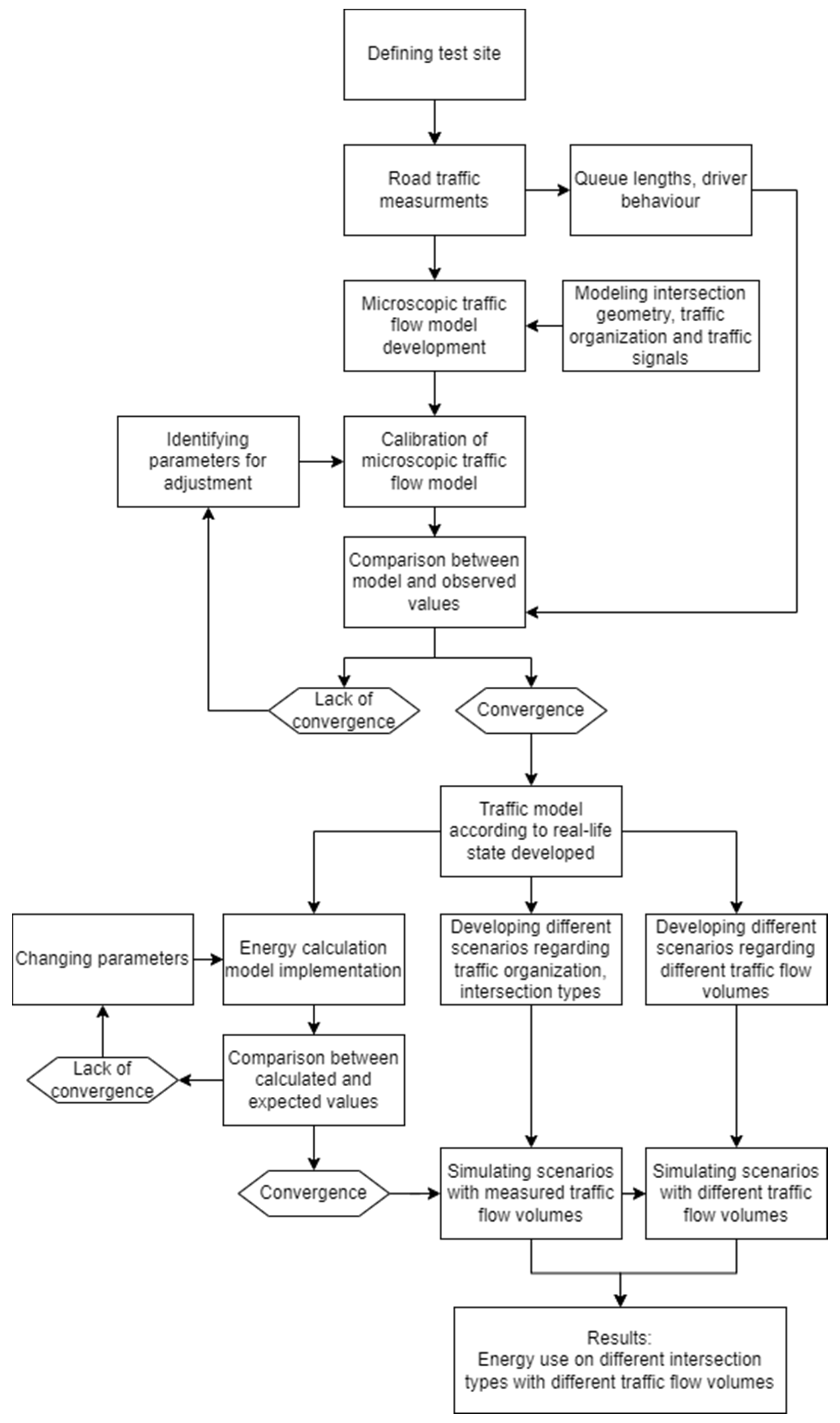
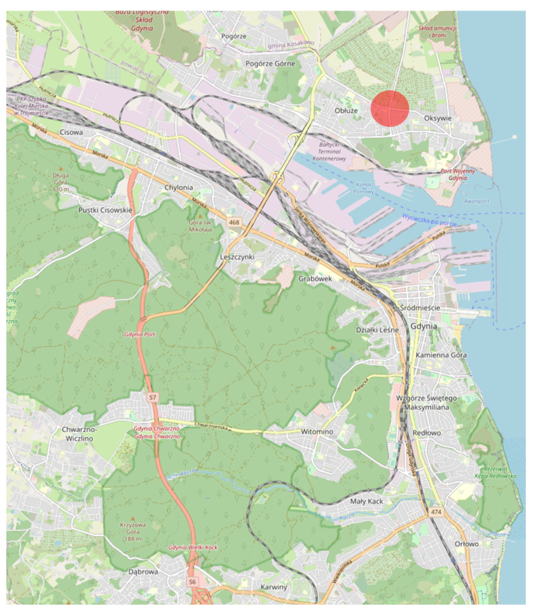
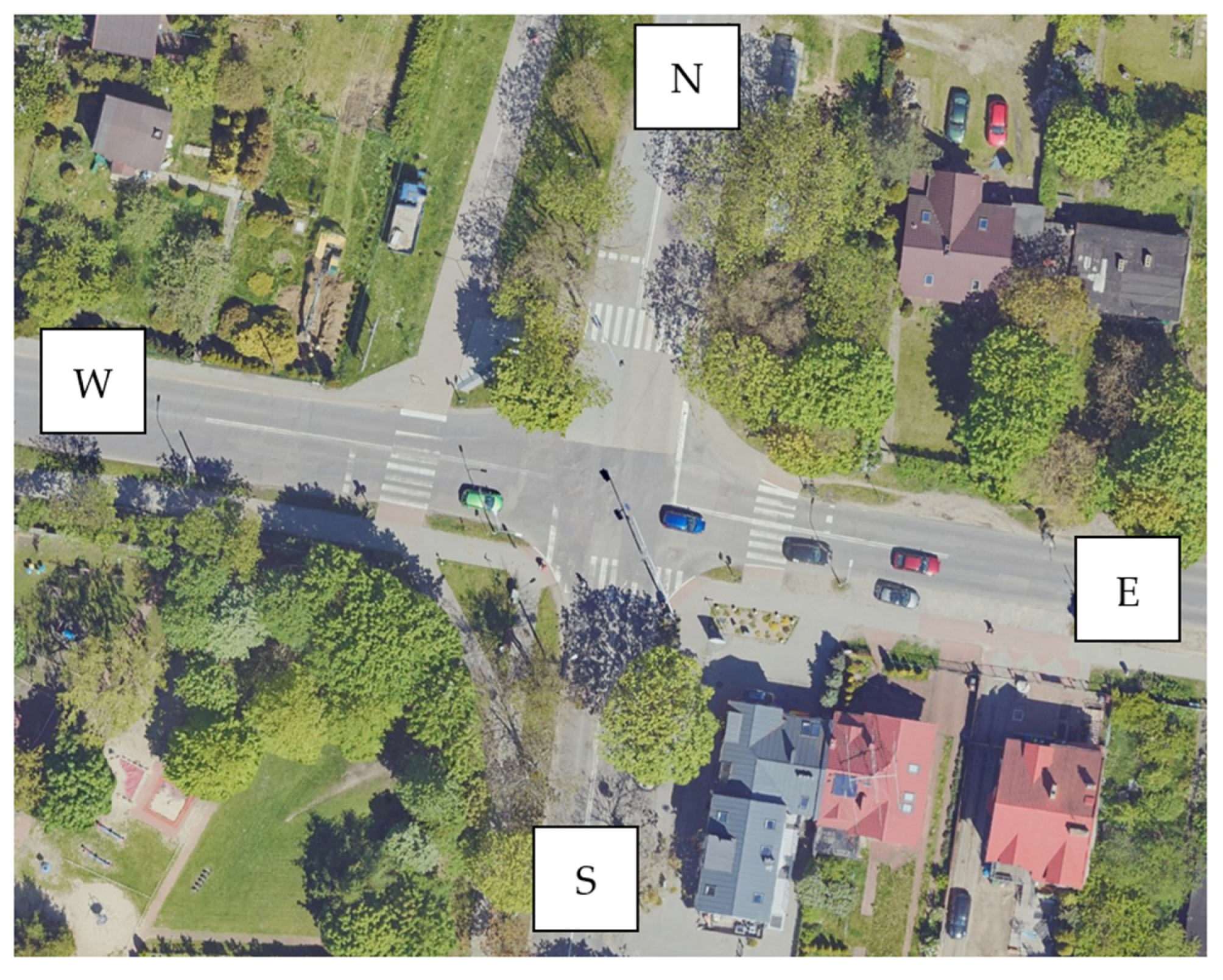
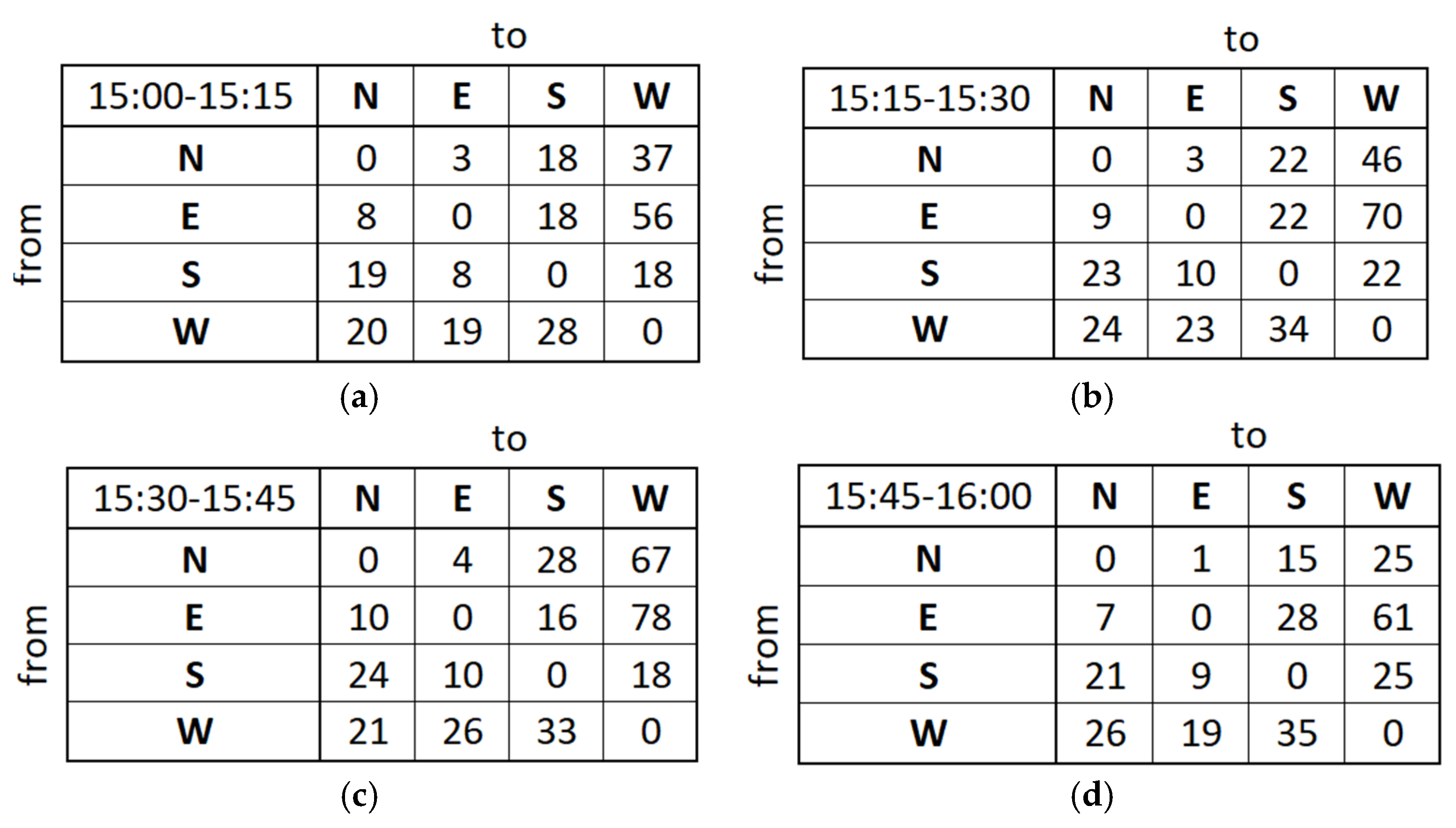
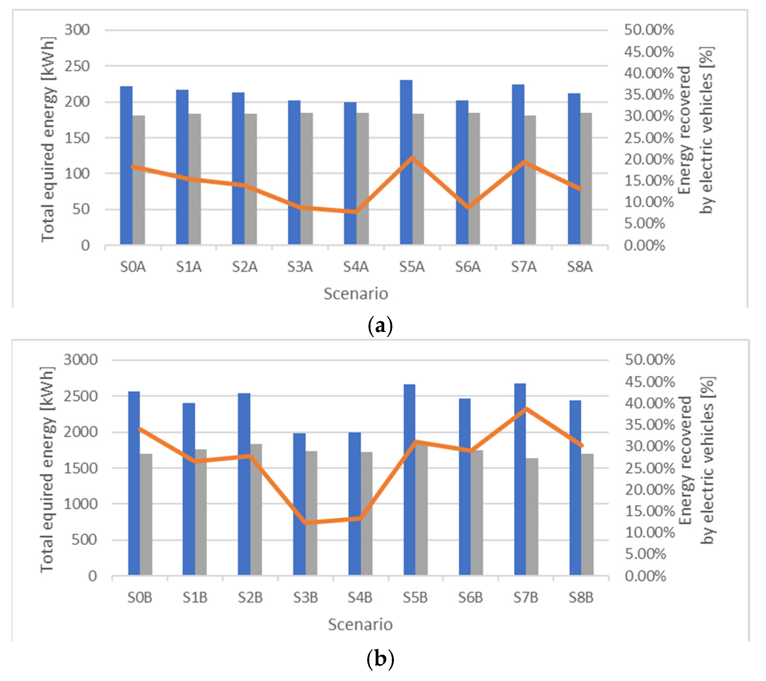
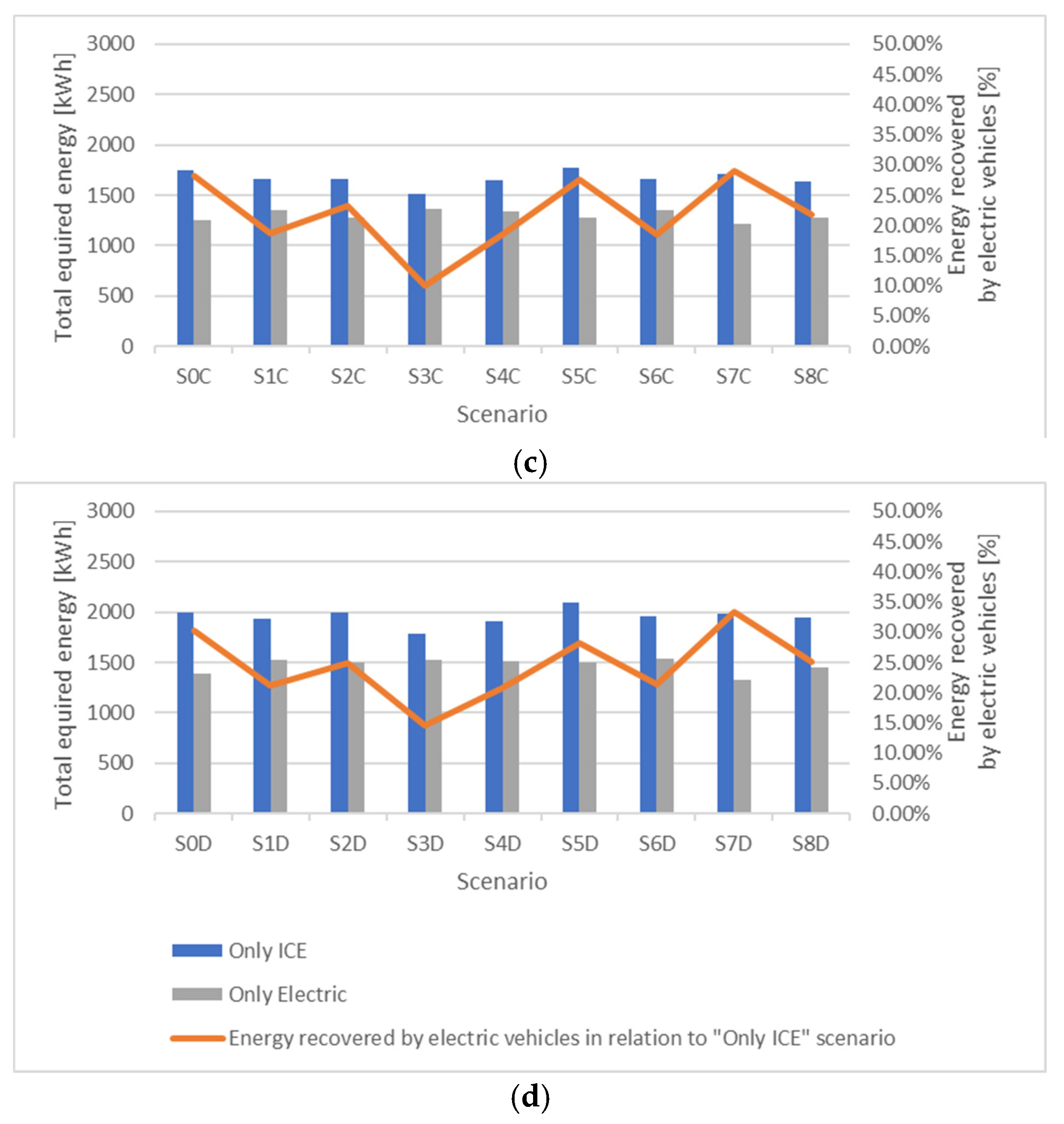
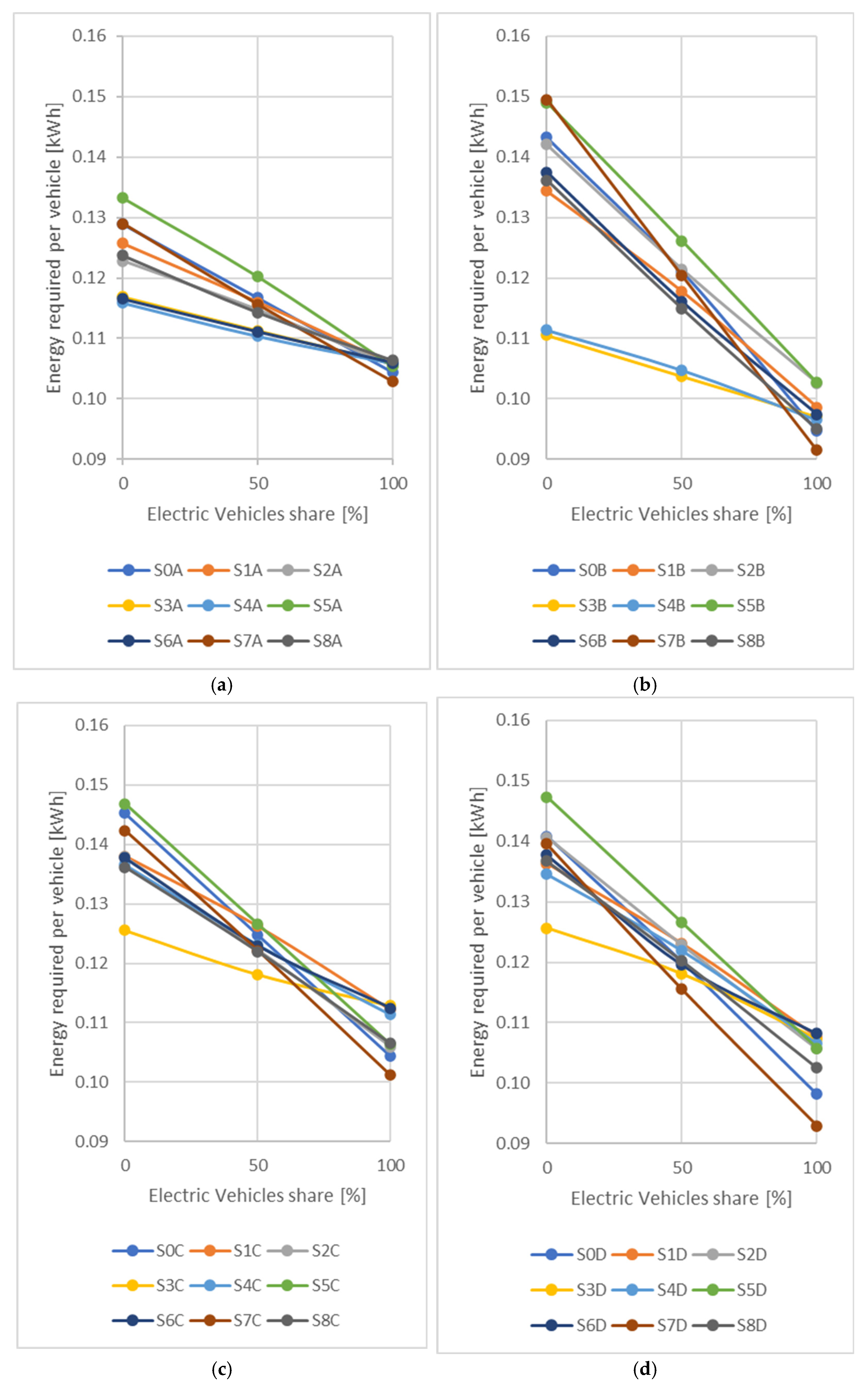
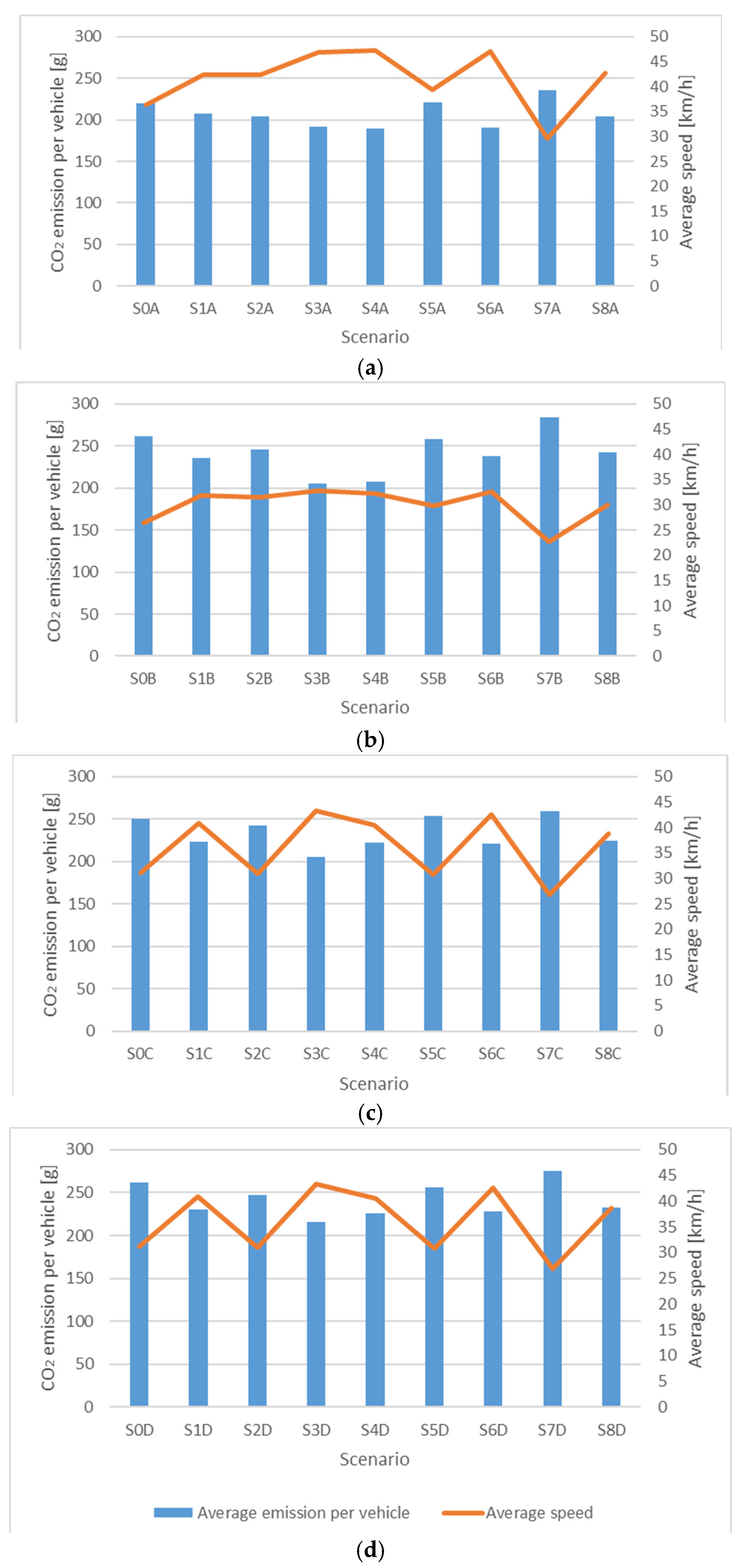
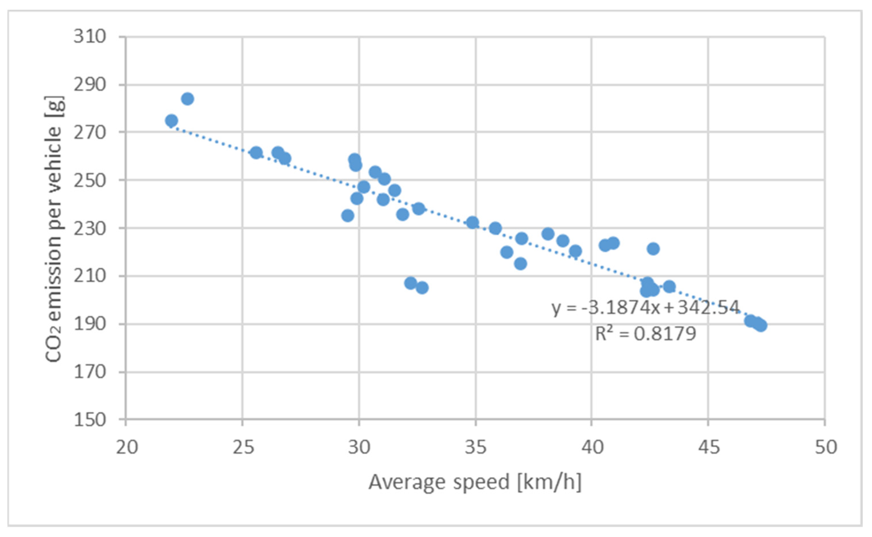