Article

Collaborative Robust Optimization Strategy of Electric Vehicles and Other Distributed Energy Considering Load Flexibility

School of Electrical & Electronic Engineering, North China Electric Power University, Beijing 102206, China
*
Author to whom correspondence should be addressed.
Energies 2022, 15(8), 2947; https://doi.org/10.3390/en15082947
Submission received: 12 March 2022 / Revised: 11 April 2022 / Accepted: 14 April 2022 / Published: 17 April 2022

Abstract

:
Aggregated electric vehicles (EVs) integrated to the grid and intermittent wind and solar energy increased the complexity of the economic dispatch of the power grid. Aggregated EVs have a great potential to reduce system operating costs because of their dual attributes of load and energy storage. In this paper, plugged-in EV is refined into three categories: rated power charging, adjustable charging, and flexible charging–discharging, and then control models are established separately; the concept of temporal flexibility for EV clusters is proposed for the adjustable charging and flexible charging–discharging of EV sets; then, the schedule boundary of EV clusters is determined under the flexibility constraints. The interval is used to describe the intermittent nature of renewable energy, and the minimum operating cost of the system is taken as the goal to construct a distributed energy robust optimization model. By decoupling the model, a two-stage efficient solution is achieved. An example analysis verifies the effectiveness and superiority of the proposed strategy. The proposed strategy can minimize the total cost while meeting the demand difference of EV users.

1. Introduction

With the increase of the proportion of renewable energy including wind power and solar energy, the inherent intermittency and volatility of renewable energy pose a new challenge to the economic dispatch of power systems [1].In addition, the number of electric vehicles (EVs) has greatly increased due to the great potential for energy conservation and emission reduction [2]. EVs have the dual attributes of load and energy storage, as the charging and discharging states and power of plugged-in EVs can be adjusted flexibly based on V2G (vehicle to grid) technology. Coordinated optimization of EVs integrated to a grid and other distributed energy sources in the system is a powerful means to maintain a more stable and economical operation of the power grid.
Based on the dual properties of EV load and energy storage, optimizing the charging and discharging process of plugged-in EVs can promote renewable energy consumption [3], maintain voltage stability [4], suppress frequency offsets [5] and reduce operating costs [6]. Reference [7] considers the combination of wind power and electric vehicles, which proves that the power imbalance in the power system can be effectively reduced, thus improving the safety of the power system. In addition, the proposed scheduling strategy reduces the operating cost of the system. In reference [8], the regulation potential of active and reactive power of EV is fully exploited, and the cooperative control strategy of electric vehicles and distributed energy is proposed, which reduces the operating cost of power systems and improves the stability of the node voltage. Reference [9] presents a novel and efficient control system for the participation of plugged-in EVs in the provisioning of ancillary services for frequency regulation.
In order to study the collaborative robust optimization strategy of EVs and other types of distributed energy, an EV control model should be established at first for its scheduling optimization. Reference [10] analyzed the rules of arrival and departure times of EVs in historical data from the perspective of user behavior patterns, established a hybrid model on the basis of EV classification, and determined the schedulable boundary of EV clusters. Reference [11] analyzed the idle, charging and discharging states and constructed a hysteresis model to describe the EV charging and discharging process. In reference [12], a virtual battery model was established from the perspective of producers and consumers to describe the boundary constraints of the charging and discharging process. In reference [13], only the physical constraints of EV power batteries were considered and the uncertainty of charging time was simulated by fuzzy numbers. In reference [14], data mining was used to analyze EV plugged-in characteristics based on a historical data set of EVs, and then the EV load model was calculated by a fuzzy model. In reference [15], the EV control process was divided into two stages: in the first stage, the Bee algorithm was used to calculate the optimal charging amount of each EV, and in the second stage, a fuzzy controller was used to distribute EV power. After reviewing the existing references, an EVs control model was established based on the same standard to describe the physical charging and discharging constraints of the power battery, which obviously ignores the preference of EV users. In the actual scene, the EV user is a highly autonomous individual who dominates the charging mode, and the unified modeling of power batteries is inevitably contradictory to the actual scene.
In view of the intermittent characteristics of renewable energy, stochastic programming [16] and opportunity constraint methods [17] are often used to deal with the uncertainty of its output. Robust optimization as a new alternative method has obvious advantages: closed convex sets are used for uncertain variables, and the optimization goal is used to ensure the robust optimal solution for any point on the convex set. In reference [18], the discrete uncertainty domain was established to find a more accurate “worst scenario” in robust optimization, and the min–max-min structural optimization model was established to realize interactive iterative solution. Reference [19] presented a robust optimal scheduling model for regional integrated energy systems to promote renewable energy consumption. Reference [20] considered the uncertainty of renewable energy output, and established a robust control model in coordination with the orderly charging of EV clusters. Reference [21] fully considered the uncertainty of EVs and formulated an optimal scheduling strategy, but it lacked consideration of the uncertainty of renewable energy power and the discharging characteristics of EVs. Reference [22] focused on collaborative robust optimization of EVs and renewable energy, proposed a robust processing method for uncertain parameters, and converted it into a mixed integer linear programming model. After reviewing the existing references, the collaborative robust optimization of EVs and other distributed energy sources is not comprehensive and does not fully take into account the discharging characteristics of EVs. In addition, when the scale of electric vehicles is large, the efficiency of solving is difficult to be guaranteed.
To sum up, there are two deficiencies in existing research: on the one hand, there are few synergistic studies between EV clusters and renewable energy, and there is a lack of in-depth discussion. On the other hand, a small number of collaborative robust optimization studies adopted a unified general EV control model without considering the demand difference in actual scenarios, and the solution complexity is relatively high, so there is a gap between existing studies and practical applications.
In this paper, an EV control model considering demand preference is established and the concept of temporal flexibility of EV clusters is proposed. The interval was used to describe the uncertainty of wind–solar output, and then the collaborative optimization robust model of EV clusters and distributed energy was established, and the model was decoupled into two stages to achieve an efficient solution. The establishment of an EV control model considering demand preference can meet the differentiated needs of users and be more consistent with the actual scene. The temporal flexibility of EV more accurately quantifies the schedulability of EV clusters. The decoupling solution strategy of the model greatly improves the solving efficiency.

2. Materials and Methods

2.1. Robust Optimal Control Framework

With the expansion of EV scale, the centralized EV control mode will become more and more complex, and EV clusters can be decentralized and optimized using the role of electric vehicle aggregators (EVAs). A simplified diagram of the optimization architecture is shown in Figure 1. In this paper, a collaborative robust optimization model of EV clusters and other types of distributed energy is established. The system contains intermittent solar and wind power energy, and EVAs carry out decentralized control of EV clusters. EVAs gather the basic parameters and demand information of EVs, including EVs’ plugged-in time, the initial state of charge (SOC) of the power battery, the expected SOC of departure, the charging mode, etc. EVAs consider the temporal flexibility constraints of the EV cluster under their jurisdiction to determine the dispatchable ability of the EV cluster. The control center considers the uncertainty of the wind and solar output in the system, formulates the optimal control strategy, and minimizes system operating costs by dispatching unit output, adjusting EVA power demand, and determining renewable energy consumption.
It should be noted that due to the energy storage properties of EVs, EV clusters can be regarded as a distributed energy storage device. When EV clusters reaches a certain scale, they can reduce or replace the energy storage capacity configuration of the system to a certain degree. Therefore, the system does not consider additional distributed energy storage devices.

2.2. EV Model and the Temporal Flexibility of EV Cluster

2.2.1. Single EV Model under Demand Difference

Differently from existing EV modeling methods, this paper establishes an EV control model with the demand difference of EV users.
From the perspective of the charging and discharging state of the power battery, the demand difference of users can be described simply. The charging mode of any plugged-in EV can be divided into three categories: rated power charging EV, adjustable charging EV and flexible charging–discharging EV. The rated power charging mode reflects the desire to minimize the time cost of the grid connection; the adjustable charging mode reflects the user’s desire to reduce economic costs and avoid excessive loss of power batteries; the flexible charging–discharging mode reflects the user’s desire to minimize the economic cost.
The three types of charging mode can reflect the demand difference of users. The three types of plugged-in EVs are modeled as follows:
(1) Rated power charging EV
For any rated power charging EV, l ,   and     t [ t l , i n , t l , o u t ] :
{ P l , t = P c , l r ,   S l , t [ S l , i n , S l , e x ) 0 P l , t P c , l r ,   S l , t S l , e x S l , t = S l , i n + n t η c , l P c , l r Δ t / E l
For any rated power charging EV, its charging power remains at the rated power until it reaches the expected SOC. In the above, t l , i n , t l , o u t , S l , i n , S l , e x , P c , l r , η c , l and E l are respectively the plugged-in time, plugged-out time, initial SOC, expected SOC, rated charging power, charging efficiency and energy storage capacity of l ; P l , t and S l , t are the actual charging power and SOC of l during the t period, respectively; Δ t is the unit duration; n t is the number of time periods of t l , i n t .
(2) Adjustable charging EV
For any adjustable charging EV, l ,   and     t [ t l , i n , t l , o u t ] :
{ 0 P l , t P c , l r   S l , t = S l , i n + n t η c , l P l , t Δ t / E l
For any adjustable charging EV, its charging power can be flexibly adjusted between zero and the rated power.
(3) Flexible charging–discharging EV
For any flexible charging–discharging EV: l ,   and     t [ t l , i n , t l , o u t ]
{ P d , l r P l , t P c , l r   S l , t S l , t h r , w h e n   P l , t < 0 ( 3 . a ) S l , t = S l , i n + n c , t η c , l P l , t Δ t E l + n d , t P l , t Δ t η d , l E l
For any flexible charging–discharging EV, it can be in a charging state or in a discharging state. Its discharging state needs to meet the discharging threshold constraints of the power battery, and the discharging power can be adjusted between zero and rated discharging power; when charging, it is equivalent to an adjustable charging EV. In the above, P d , l r and η d , l are the rated discharging power and discharging efficiency of l , respectively; n c , t and n d , t are the number of charging and discharging periods of t l , i n t , respectively; S l , t h r is the discharging threshold, and formula ( 3 . a ) restricts the SOC of the discharging process to be no less than S l , t h r .
The above three types of plugged-in EVs are referred to as Type 1, Type 2, and Type 3, respectively.

2.2.2. Temporal Flexibility for EV Clusters

Due to the driving characteristics of EVs, it is necessary to ensure the user′s electricity demand. Any EV must meet that the actual SOC is not lower than the expected SOC value when the EV is plugged out, which is S o , l S l , e x . Taking the expected energy reaching E l , e x when the EV is plugged out as an example, the scheduling capacity diagrams of Type 2 and Type 3 EVs are shown in Figure 2.
In the figure, E l , i n , E l , e x and E d , t h r are the initial electric quantity, the expected electric quantity of departure time and discharging electric quantity threshold of l , respectively. As shown in Figure 2, the broken line indicates the change of E l , t , E l , t = E l S l , t . The broken line, abc, is the actual change track of the electric quantity. ab1c is the trajectory of the rated charging EV, and aa1c is the trajectory formed by charging to the desired SOC in the latest charging period [ t d , t l , o u t ] . These constitute the upper and lower boundaries, respectively.
For Type 2 and Type 3 EVs, it is not accurate to determine the schedulable capacity only based on the model Equations (2) and (3) established in Section 2.1, and further consideration should be given to flexibility constraints. For the adjustable charging EV, as shown in point b in Figure 2a, the time period [ t x , t y ] represents the maximum idle time ( P l , t = 0 ) of l . For the flexible charging–discharging EV, as shown in point b in Figure 2b, similarly, when l is not in the discharging state, period [ t x , t y ] represents the maximum idle time of l ; when l is in the discharging state, the line with slope P d , l r from point b to the lower boundary is made, and E d , l represents the maximum discharging capacity in periods [ t x , t m ] ( t m < t y ). When t y < t t l , o u t , both the adjustable charging EV and the flexible charging–discharging EV maintain P c , l r charging to ensure electricity demand, and the schedulable capacity is reduced to zero.
Based on the above analysis, for t x ( t l , i n t x < t l , o u t ) , the electricity demand of Type 2 and Type 3 EVs that can be reduced during periods [ t x , t y ] is calculated by Equations (4) and (5):
Δ E l , m a x P l , t ( t y t x )
{ Δ E l , m a x P l , t ( t y t x ) + E d , l E d , l = P c , l r ( t l , o u t t m ) + E l , t x E l
Supposing T is the optimized time domain, the total power P e v , t of the EV cluster in the t ( t T ) period can be calculated as:
P e v , t = o = 1 N A ( i = 1 N x o P i , t o + j = 1 N y o P j , t o + k = 1 N z o P k , t o )
where N A is the number of EVAs; N x , N y and N z are the numbers of the three types of EV. Equation (6) satisfies the constraints of Equations (1)–(3).
The electricity demand of the EV cluster during the period t , t T can be adjusted down to the accumulation of Type 2 and Type 3 EVs:
{ Δ E s , t o = 1 N A ( Δ E 2 , t o + Δ E 3 , t o ) Δ E 2 , t o = j = 1 N y o min ( P l , t o Δ t , Δ E j , max o ) Δ E 3 , t o = k = 1 N z o min [ ( P l , t o + P d , l o ) Δ t , Δ E k , max o ]
Equation (7) quantifies the dispatchable capacity of the EV cluster. Meanwhile, Equation (7) should satisfy the constraints of Equations (2) and (3).
It should be pointed out that Equation (7) only represents the maximum down-regulation capability of EV clusters. For any Type 2 and Type 3 EVs, the maximum up-regulation capability can be adjusted to P c , l r .
It can be seen that Formula (7) gives the overall adjustable boundary of the EV cluster. In the process of optimization, the EV cluster is regarded as a whole to solve the optimal power of the EV cluster and avoid focusing on a single EV, which can accelerate the optimization process [23].
Because the schedulable boundary calculation of EV clusters is based on the flexibility constraints of Type 2 and Type 3 EVs, this article calls it the temporal flexibility of EV clusters. EV cluster temporal flexibility is determined based on the broken line abc. In actual scenarios, the charging trajectory abc of the Type 2 or Type 3 EVs can be determined by existing methods, such as maximizing the interests of the user or balancing the interests between grid operator and users [24].

2.3. Robust Optimization Model Considering Temporal Flexibility

2.3.1. Robust Optimization Theory

Considering the random volatility of wind power and solar power, the optimal operation strategy can reduce the system reserve demand, reduce the operation cost, and promote the consumption of renewable energy. In recent years, the two-stage robust optimization model with a min–max structure was proposed. The main feature is to find the “worst scenarios” and determine the optimal operation plan under the “worst scenarios”. The robust model of the min–max structure can be expressed by Equation (8):
{   max ζ D   min X   F ( X , ζ ) s . t . { H ( X , ζ ) = 0 G ( X , ζ ) 0
where X is the decision variable. ζ and D are its uncertain parameters and uncertain sets, respectively. F ( X , ζ ) is the optimization objective function. H ( X , ζ ) is the equality constraint; G ( X , ζ ) is the inequality constraint. The essence of Equation (8) is to minimize the optimization target F by optimizing decision variable X under the influence of the uncertain parameter ζ .

2.3.2. Construction of Robust Optimization Model

The objective function is constructed with the goal of minimizing costs. The system contains two types of renewable energy: solar and wind power. In order to simplify the complexity of the model and promote the consumption of renewable energy, the cost of abandoning wind and solar is included in the objective function.
max ζ D   min C s = C g ( P g ) + C b ( P b ) + C a ( E s ) + C q ( W )
The essence of Formula (9) is to minimize the cost on the uncertain set D . P g , P b , E s and W are the unit power vector, standby power vector, EV cluster power vector, and abandoning renewable power vector, respectively. C g , C b , C a and C q are the corresponding cost functions; the calculation methods are as follows:
(1) Unit operating cost:
C g ( P g ) = t = 1 N t i = 1 N g u i , t ( a i + b i P g i , t + c i P g i , t 2 ) + t = 2 N t i = 1 N g ( u i , t u i , t 1 ) s i
Formula (10) contains two parts of cost: fuel cost and start–stop cost of units, where N g is the number of units; N t is the number of optimization periods, N t = T / Δ t ; a i , b i and c i are the cost coefficients of the i-th ( i N g , i N + ) unit; u i , t is the boolean variable that indicates the startup and shutdown of the unit i at period t ; s i is the startup and shutdown cost of unit i .
(2) Standby power capacity cost:
{ C b ( P b ) = t = 1 N t i = 1 N g ( γ i u p P g i , t u p γ i d o w n P g i , t d o w n ) P g i , t u p P g i , t d o w n = 0   ,     i , t ( 11 . a )
The essence of Formula (11) is the dispatching cost of standby power capacity, which includes up-regulated and down-regulated costs, where P g i , t u p , P g i , t d o w n , γ i u p and γ i d o w n are respectively the up-regulated and down-regulated powers of unit i and the corresponding adjusted prices; Formula ( 11 . a ) restricts P g i , t u p and P g i , t d o w n both to be zero or only one to be not zero at the same period.
(3) EV cluster compensation cost:
{ C a ( E s ) = C d + C m C d = o = 1 N A ( j = 1 N y o c j o + k = 1 N z o c k o ) C m = t = 1 N t β t Δ E s , t Δ t
C d 
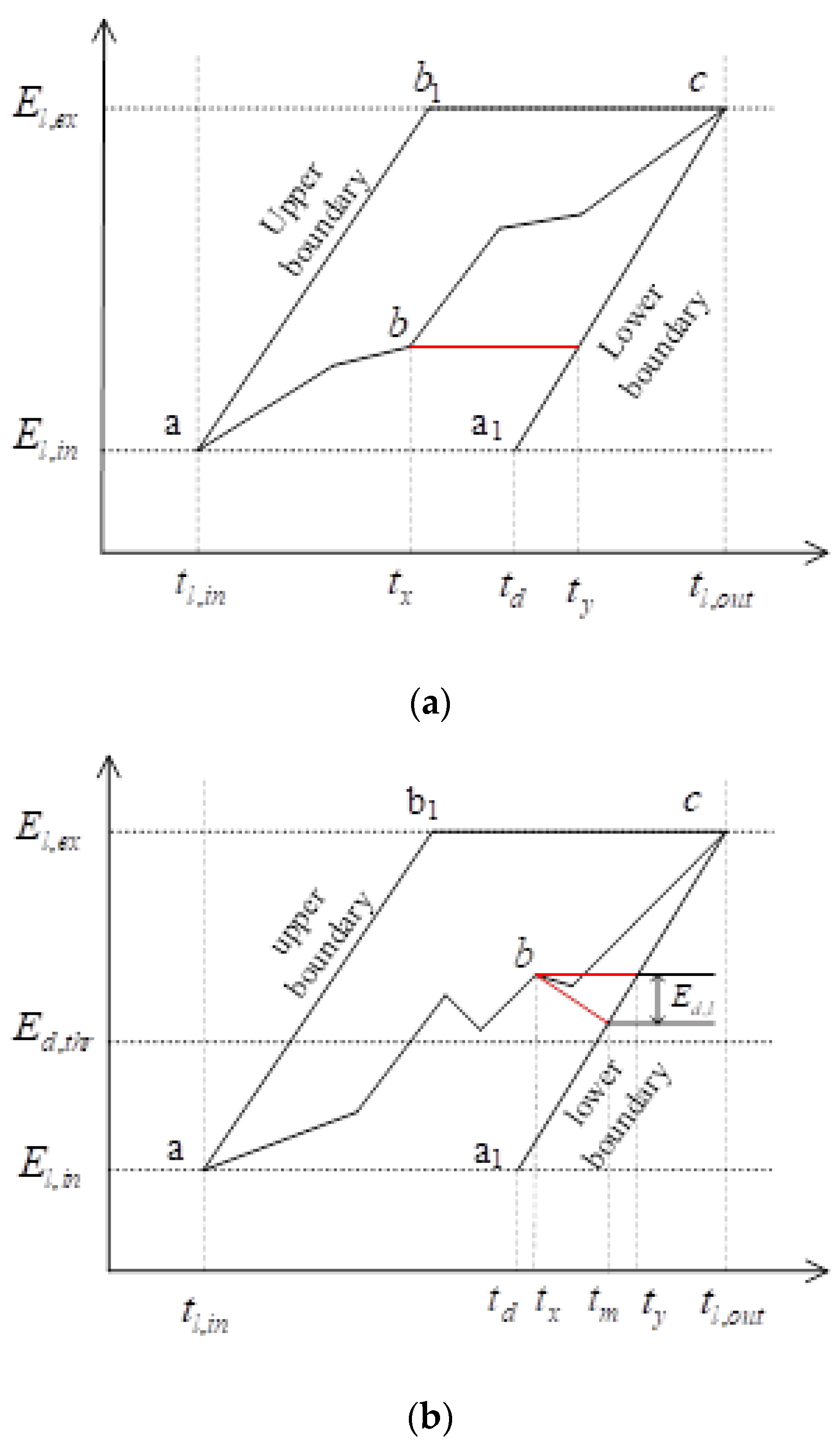
is the compensation cost of the EV cluster, which corresponds to the broken line abc of Type 2 and Type 3 EVs in Figure 2; C m is the power adjustment compensation cost of the EV cluster in response to intermittent fluctuations of renewable energy; β t is the compensation factor. c j o and c k o are respectively the incentive cost of the j - th Type 2 EV and the incentive cost of the k - th Type 3 EV in the o - th EVA. To calculate the incentive cost c l of l , this paper uses the method of reference [25]:
c l = s l , max s l s l , max c l , max + φ E l
Formula (13) shows that the closer the charging trajectory of the EV is to the upper boundary, the smaller the compensation cost is, where s l , max and c l , max are respectively the charging benefit and cost corresponding to the upper boundary of l (broken line a b 1 c ); s l is the charging benefit corresponding to the broken line a b c ; φ and E l are respectively the discharging compensation coefficient and the total discharging energy.
(4) Cost of abandoning renewable energy:
{ C q ( W ) = t = 1 N t λ Δ W t Δ t Δ W t = P ˜ s , t + P ˜ w , t + ζ t P s w , t ζ t = θ s , t + θ w , t
where Δ W is the power of abandoning renewable energy; λ is the penalty factor; P ˜ s , t , P ˜ w , t , θ s , t and θ w , t are the forecast output values and forecast errors of solar and wind power, respectively; P s w , t is the actual consumption of renewable energy.
The solution of objective function Equation (9) needs to meet the constraints of unit operation and power balance.
(1) Unit operation constraints:
{ P g i min P g i , t + P g i , t u p P g i max P g i min P g i , t + P g i , t d o w n P g i max 0 P g i , t u p P g i u m a x P g i d m a x P g i , t d o w n 0     i , t
{ P g i min P g i , t P g i max P g i , t P g i , t 1 P g i u m a x P g i , t 1 P g i , t P g i d m a x ( u i , t 1 u i , t ) ( t i , o n T i , o n ) 0 ( u i , t u i , t 1 ) ( t i , o f f T i , o f f ) 0   i , t
where P g i min , P g i max , P g i u m a x and P g i d m a x are the maximum and minimum outputs of unit i , and the limit value of output increase and decrease, respectively; t i , o n , t i , o f f , T i , o n and T i , o f f are the continuous start-up and shutdown time, and the minimum start-up and shutdown time of unit i , respectively.
(2) Power balance constraint:
i = 1 N g P g i , t + P s w , t + i = 1 N g P g i , t u p i = 1 N g P g i , t d o w n = P e v , t + P L

2.3.3. The Description of Output Uncertainty Convex Set

The selection of the uncertain parameter ζ t in Formula (9) has a direct impact on the optimization results. This article uses intervals to describe the volatility of wind and solar output. Let the interval of θ s , t and θ w , t be:
{ θ s , t : [ P _ s , t P ˜ s , t , P ¯ s , t P ˜ s , t ] θ w , t : [ P _ w , t P ˜ w , t , P ¯ w , t P ˜ w , t ]
Formula (13) represents the fluctuation range of uncertain parameters, where P ¯ s , t and P _ s , t are respectively the upper and lower limits of solar power at period t ; and P ¯ w , t and P _ w , t are respectively the upper and lower limits of wind power at period t .
According to the interval calculation rule, the uncertainty interval of renewable energy output ζ t is [ P _ s , t + P _ w , t P ˜ s , t P ˜ w , t , P ¯ s , t + P ¯ w , t P ˜ s , t P ˜ w , t ] . Introducing the { 0 , 1 } binary auxiliary variable z t + , z t and the robust model conservative degree control parameter Γ , the uncertainty of renewable energy output under robust control is described by Equation (19):
{ D : { P ˜ s , t + P ˜ w , t + z t + ( ζ ¯ t ζ t ) z t ( ζ t ζ _ t ) } ζ ¯ t = P ¯ s , t + P ¯ w , t P ˜ s , t P ˜ w , t ζ _ t = P _ s , t + P _ w , t P ˜ s , t P ˜ w , t z t + + z t 1 , t ( 19 . a ) t = 1 N t z t + + z t Γ ( 19 . b )
where ζ ¯ t and ζ _ t are the upper and lower limits of ζ t , respectively; z t + and z t control whether ζ t obtains the upper limit or the lower limit; for z t + = 1 , z t = 0 , ζ t takes the upper limit of the interval; for z t + = 0 , z t = 1 , ζ t takes the lower limit of the interval; when both are 0, it means that both wind and solar output take the predicted value ( P ˜ w , t , P ˜ s , t ). When Γ = 0 ( Γ [ 0 , N t ] ), it indicates that the wind and solar output in all periods are predicted values, and the output volatility is not considered, and the model is the most aggressive; when Γ = N t , it indicates that the upper or lower limit of ζ t is used for all periods, and the model is the most conservative. In practical applications, the conservative degree of the model is controlled by adjusting the value of Γ .

2.3.4. Decoupled Solving of Robust Optimization Models

The models in Section 2.2 and Section 3.2 of this paper can decouple the objective function Equation (9) into two stages. First stage: when volatility is not considered and the forecast output of wind power and solar power is based on the minimum cost, the optimal output of the unit, the power of the EV cluster, and the consumption of renewable energy in the period T are determined with the goal of minimum cost. Second stage: when considering the fluctuation of renewable energy, according to the given Γ value, the solution value of the first phase is adjusted again with the goal of minimum adjustment cost.
max ζ D   min C s = min ζ ˜ [ C g ( P g ) + C a ( E s ) + C q ( W ) ] f i r s t   s t a g e + max ζ D   min [ C b ( P b ) + C a ( E s ) + C q ( W ) ] s e c o n d   s t a g e
Equation (20) needs to satisfy constraint Equations (1)–(3), (7), (10)–(17).
(1) First stage solution
The first stage is the deterministic minimization problem. C m = 0 , and θ s , t and θ w , t are both equal to zero;
u i , t , P g i , t , P e v , t , P s w , t are decision variables; let X be the optimization vector in the whole T period, then X = [ u , P g i , P e v , P s w ] T , and the dimension of X is 2NgT + 2T. The matrix form of the min term is as follows:
  min A X s . t . { H ( X ) b   G ( X ) = 0
where A is the corresponding coefficient matrix; H ( X ) and G ( X ) respectively correspond to the inequalities and equality constraints of Equations (1)–(3), (10), (12), (14), (16) and (17); b is a suitable constant vector; 0 is a zero vector. Equation (21) is a typical mixed integer programming problem, which is solved efficiently by using the commercial solver CPLEX.
(2) Second stage solution
The second stage can be called the reschedule minimization problem, C d = 0 ; C b ( P b ) contains the non-convex constraint of Equation ( 11 . a ), and it is difficult to solve directly. In order to relax the constraints of Formula (9), we construct function Formula (22) as follows:
max Z   min Y   f = [ C b ( P b ) + C a ( E s ) + C q ( W ) ] + t = 1 T { | i = 1 N g γ i u p P g i , t u p | + | i = 1 N g ( γ i d o w n + γ i u p ) P g i , t d o w n | }
It satisfies constraint Equations (4)–(7), (11), (12), (14)–(19). A brief proof of the constraint of relaxation Formula ( 11 . a ) is as follows:
Let b t = i = 1 N g P g i , t u p , c t = i = 1 N g P g i , t d o w n ( t T ) ; suppose the optimal solution in period t is δ t ( δ t = b t c t , and δ t 0 or δ t < 0 ). Let x 1 > 0 , x 2 < 0 , and construct function g as follows:
min g ( b t , c t ) = ( x 1 b t + x 2 c t ) + x 1 | b t | + ( x 2 + x 1 ) | c t |
From the perspective of power balance, if δ t 0 , there are only two possibilities for b t , c t values:
(1) b t > 0 , c t < 0
(2) b t > 0 ,   c t = 0
Let b t = δ t + m 1 , c t = m 1 ( m 1 0 ). m 1 > 0 and m 1 = 0 correspond to the above two possibilities, respectively; b t and c t are put into Equation (23) to obtain g ( δ t + m 1 , m 1 ) = 2 x 1 δ t + 3 x 1 m 1 . Obviously, g ( δ t , 0 ) g ( δ t + m 1 , m 1 ) , that is, g ( b t , 0 ) g ( b t , c t ) , so when δ t 0 and c t = 0 , Equation (23) obtains the optimal value. Similarly, if δ t < 0 , when b t = 0 , Equation (23) obtains the optimal value.
Therefore, when Formula (23) takes the optimal solution, B = 0 is satisfied during any period, that is, b t c t = 0 is satisfied for any unit.
P g i , t u p , P g i , t d o w n , Δ E s , t , P s w , t and z t + , z t are decision variables. Let Y = [ P u p , P d o w n , Δ E s , P s w ] T , Z = [ z + , z ] T ; the dimension of Y is 2NgT + 2T; the dimension of Z is 2T. The general form of the matrix of Equation (22) is:
max Z   min Y   B Y   s . t .   { M 1 Y + N 1 Z L M 2 Y + N 2 Z 0
where B is the corresponding coefficient matrix; both M and N are matrices adapted to Formulas (7), (11), (12), (14)–(19); L is a suitable constant vector; 0 is a zero vector. Max-min is a two-level optimization problem. According to the duality theory, dual variables μ and ρ are introduced to convert the two-level optimization into a single-level optimization. The dual form of Equation (24) is:
max Z , μ , ρ L T μ + Z T ( N 1 T μ + N 2 T ρ ) s . t . { M 1 T μ + M 2 T ρ + B T = 0 μ 0 ρ R
Equation (25) is a linear programming problem, which is solved by using the simplex method. Equation (24) satisfies strong duality; let Z * , Y * and Z * , μ * , ρ * be the optimal solutions of Equations (24) and (25), respectively; it meets: B Y * = L T μ * + Z * T ( N 1 T μ * + N 2 T ρ * ) .
According to the complementary relaxation in the KKT condition, M 1 Y × μ = 0 can be obtained, which can be further accelerated by introducing it into Equation (25).
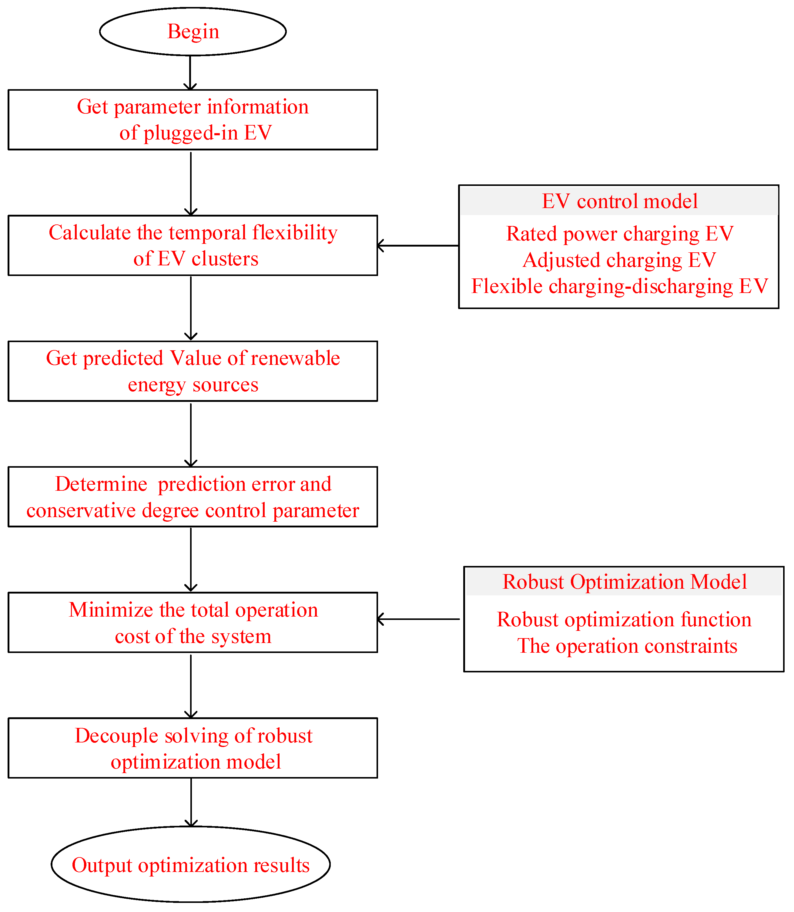
The flowchart in Figure 3 summarizes the whole process of the proposed model.

3. Results and Discussion

3.1. Data Description and Parameter Setting

The optimization domain is 24 h, the per step is 15 min, and there are 96 time periods in a day; the number of units is 3; the proportion of the three types of EVs is 0.2, 0.3, 0.5; the probability distribution of EVs and plugged-out time and daily mileage are taken from reference [26] and reference [27]; the renewable energy output and the base load curves are taken from the area of Belgium [28] (reduced in equal proportions); the penalty factor of abandoning renewable energy is taken from the literature [29]; a Monte Carlo simulation was used to generate EVs’ arrival time, departure time, and initial SOC; the expected value of SOC was set to be 0.95; the market electricity price and value are shown in Appendix A, Table A1; the basic parameters of units and EV are shown in Appendix A, Table A2 and Table A3. Appendix A, Figure A1, shows the predicted output of renewable energy; Appendix A, Figure A2, shows the number of the three types of EVs in 96 periods. In order to facilitate the calculation, in Section 3.3, a symmetric interval was used for θ w , t and θ s , t , and the prediction error was set to be 5%, and then the upper and lower limits of the renewable energy output were 1 + 5% and 1–5% times the predicted value, respectively.
Both the output predicted value and the prediction error can be improved by the deep learning method to improve the prediction accuracy, which can further improve the superiority of the robust model.

3.2. Robust Optimization Results Analysis

Taking the value of Γ as 18, and setting the prediction error to 5% for both wind power and solar power, Figure 4 shows the results of robust optimization of EV cluster power; the black curve in Figure 4 is the EV cluster power solved in the first stage, the red curve is the final power curve of EV cluster after the second stage optimization, and the gray area is the adjustable interval of EV cluster under the temporal flexibility constraint.
As can be seen from Figure 4, the EV cluster power decreases in specific periods after robust optimization. However, the EV cluster power is increased in some periods due to the temporal flexibility constraint and the total electricity demand constraint, while the EV cluster power remains unchanged in other time periods. The decoupled two-stage solution avoids re-optimization for all periods and improves the solution efficiency.
Figure 5 shows the power output of the three units in 96 periods after the first stage optimization. Figure 6 shows the unit cost and EV cluster compensation cost after the first stage optimization. The abandoning renewable costs are zero after the first stage solution, indicating that the renewable energy is completely consumed based on the model proposed in this paper. From the analysis of the proposed model, we can see that Equation (17) incorporates the renewable energy consumption into the power balance, and the penalty factor of abandoning renewable energy in Equation (14) takes a large value; the EV cluster has sufficient scale to ensure that the renewable energy is completely consumed.
Combined with the analysis in Figure 7 and Table 1, the cost of the EV cluster in the first stage is CNY 28.928 × 10⁴, which is the compensation cost of Type 2 and Type 3 EVs. The power adjustment costs of the three units and EV cluster in the second stage in response to the fluctuation of renewable energy are CNY 2.467 × 10⁴, CNY 1.394 × 10⁴, CNY 0.352 × 10⁴ and CNY 3.051 × 10⁴, respectively. DG1 generates the highest cost, indicating that the power adjustment of DG1 is the largest. Based on the model established in this paper, the second stage also ensures that the renewable energy is fully consumed.
To further verify the applicability and superiority of the model in this paper, the following different schemes are used for comparison.
Scheme 1: The demand difference was considered, that is, all plugged-in EV are considered as flexible charging–discharging EVs, and the temporal flexibility constraint was not considered.
Scheme 2: The demand difference was not considered, but the temporal flexibility constraint of EV clusters was considered.
Scheme 3: The demand difference was considered, but the temporal flexibility constraint of EV clusters was not considered.
Scheme 4: Both the demand difference and the temporal flexibility constraint of EV clusters were considered.
Schemes 1–4 adopt the decoupling solution method proposed in this paper. The percentage of three types of EVs and the total number of EVs are kept the same under the four schemes. Obviously, the upper bound of the adjustable interval of EV cluster under the four schemes is consistent, and the results of the lower boundary solution under the four schemes are shown in Figure 8.
From Figure 8, it can be seen that the lower bound of EV cluster power is lower for Schemes 1–3 compared with Scheme 4. This is because Schemes 1 and 2 do not consider the demand difference of EV users; both are considered as flexible charging–discharging EVs, and the adjustable power interval of the solution is larger, but there is an inevitable contradiction to the realistic scenario. The lower bound of EV cluster power obtained from Scheme 3 is smaller than that of Scheme 4. This is because the solution method considering the temporal flexibility constraint quantifies the dispatchable capacity of EV clusters in a more precise way under the premise of ensuring the EV power demand, which means that the lower bound of the EV cluster obtained is slightly higher but more accurate.
Schemes 1–4 all use the two-stage decoupling optimization solution method established in this paper. In comparison, Scheme 5 uses the “worst scenario” robust method.
Scheme 5: Both the demand difference and the temporal flexibility constraint of EV clusters were considered, and the “worst scenario” robust method is adopted in the solving process.
Figure 9 gives the optimization results of the five schemes under different prediction errors of the renewable output; Table 2 shows the corresponding solution times. The cost of Schemes 4 and 5 are CNY 105.41 × 10⁴ and CNY 109.57 × 10⁴, respectively, under the prediction error of 5%. The solving time of Schemes 4 and 5 are 442.8 and 523.2 s, respectively, under the prediction error of 5%.
Analyzing Figure 9 and Table 2 together, when the prediction error is 5% or 10%, the robust solution results of Schemes 1–5 are basically the same because of the enough adjustable power of EV cluster and more accurate prediction of renewable energy. However, different schemes for individual EVs must be different, and without considering the demand difference of users, the users’ satisfaction will decrease. As the prediction error increases, the cost of Schemes 1 and 2 is significantly lower than that of Schemes 3 and 4, because Schemes 1 and 2 obtain a larger adjustable power interval of the EV cluster; the solution results of Schemes 4 and 5 are similar under different prediction errors, but the solution of Scheme 5 is more time-consuming.

3.3. Analysis of EV Charging Process

Let A k ( k = 1 , 2 , 3 , 4 ) be the kth EVA, and let D m , k ( m = 1 , 2 , 3 ) be the set of Type m EV in the kth EVA. In order to visualize the demand difference of the three types EV, one EV is randomly selected in D m , k , which is denoted as l m , k ( l m , k D m , k ) . The change curve of SOC for the 12 EVs is shown in Figure 10.
The SOC of the three EV types in A1–A4 is above 0.95 during their departure, which ensures the electricity demand of EV users. No matter when the l 1 , k is connected to a grid, it is charged to the desired SOC at the rated charging power; during the plugged-in periods of l 2 , k , the actual charging power is less than the rated charging power, and the SOC growth is slower, but l 2 , k is not in the discharging state during the plugged-in periods; during the plugged-in periods of l 3 , k , a few periods are in the discharging state, but it is guaranteed that the SOC is not lower than the 0.5 threshold during the discharging process, such as vehicle l 3 , 3 . It should be noted that the charging and discharging states of EV in sets D 2 , k and D 3 , k are also constrained by the user′s plugged-in duration. However, in order to meet the user′s electricity demand, the EVs in sets D 2 , k and D 3 , k will still approach the rated charging power because of their shorter connection time, such as l 2 , 2 and l 3 , 4 in Figure 10.
From the perspective of time-of-use electricity price, the EVs in the D 2 , k and D 3 , k sets have higher charging power when the electricity price is lower, which is beneficial to reduce the plugged-in cost of EV users. Obviously, the optimization model established in this paper fully guarantees the demand difference of EV users.

3.4. The Influence of Prediction Error and the Value of Γ on Robust Optimization

Section 3.2 and Section 3.3 are based on the premise that the prediction error is 5% and the value of Γ is 18. However, in practice, due to the limitation of prediction technology, the prediction accuracy of 5% may not be guaranteed. In order to verify the applicability of the robust optimization model proposed in this paper, the prediction errors are taken as 5%, 10%, 15%, 20%, 25%, and 30%. Γ takes 1 as a step and takes a value in the interval [1, 96]. The relationship between the optimization total cost and the prediction error and conservatism is shown in Figure 11.
As shown in Figure 11, the higher the model conservativeness and the lower the prediction error of renewable energy, the higher the total robust cost. When the prediction accuracy is higher, the total robust cost grows more slowly with the increase of model conservativeness, and grows more sharply when the prediction accuracy is lower; when the model conservativeness is lower, the total robust cost grows more slowly with the decrease of prediction accuracy, and grows more sharply when the model conservativeness is higher.

3.5. The Impact of the Proportion of Three Types EV on Robust Optimization

The ratios of three EV types in Section 3.2, Section 3.3 and Section 3.4 are all 2:3:5, and this section discusses the effect of different EV ratios on robust optimization. Based on the EV control model with demand difference in Section 2, only the power of Type 2 and Type 3 EVs can be cut or in the discharging state, and the effect of the three EV types on robust optimization is equivalent to the effect of Type 2 and Type 3 EV ratios on robust optimization. Keeping the value of Γ and the size of EV cluster constant, let the Type 2 and Type 3 EV ratios be r e . Both r e in the interval of [0, 1] and the prediction error in the interval of [0, 30%] are taken in equal intervals of 0.01 steps, and the total cost is shown in Figure 12.
With the increase of the proportion of Type 2 and Type 3 EVs, the total robust optimization cost gradually decreases, and when it increases to a sufficient EV cluster schedulable capacity, the total robust cost decreases gradually. As the forecast error of renewable increases, higher Type 2 and Type 3 EV ratios are required to minimize the total robust cost. When all EVs are Type 1 EVs, the total robust cost is CNY 25.531 × 10⁵; when all EVs are Type 2 or Type 3 EVs, the total robust cost is CNY 10.137 × 10⁵.

4. Conclusions

This paper proposes a collaborative robust optimization strategy of EVs and other distributed energy considering load flexibility. The following conclusions can be drawn from the research:
(1) The robust optimization strategy takes into account the demand preference of EV users. The plugged-in EVs are divided into three categories: rated power charging EVs, adjustable charging EVs, and flexible charging–discharging EVs. The three categories of EVs map the different needs of users, which better match the actual scenarios.
(2) A robust optimization model was proposed and the decoupling calculation of the model was realized. The proposed model can obtain a smaller robust cost and higher computational efficiency. The robust total cost and computational efficiency are CNY 105.41 × 10⁴ and 442.8 s, respectively. Compared with other methods, the robust total cost and computational efficiency are reduced about by 3.8% and improved by about 15.4%, respectively.
(3) The robust optimization results were tested when the conservative degree control parameter was set at different values between 0 and 96, the prediction error was set at different values between 0 and 30%, and the proportion of dispatchable EV was set at different values between 0 and 100%. The validity of the proposed model was further verified, and theoretical guidance was provided for the selection of coefficient values in practical application.
It should be pointed out that only the uncertainty of renewable energy output is considered in this paper and the uncertainty of EVs should not be ignored. Thus, the uncertainty of EVs needs to be further considered, and a collaborative analysis model of EV uncertainty and renewable energy uncertainty should be established in the further research.

Author Contributions

The contributions of the authors are summarized as follows. Conceptualization, Y.W. and B.Z.; methodology, Y.W.; software, C.L.; validation, Y.W., B.Z. and C.L.; formal analysis, B.Z.; investigation, C.L.; resources, Y.W.; data curation, B.Z.; writing—original draft preparation, Y.W.; writing—review and editing, B.Z.; visualization, Y.H.; supervision, Y.H.; project administration, Y.H.; funding acquisition, Y.H. All authors have read and agreed to the published version of the manuscript.

Funding

This research was funded by the Science and Technology Project of State Grid, grant number SGJSDK00JLXT7118041.

Conflicts of Interest

The authors declare no conflict of interest.

Abbreviations

The following abbreviations are used in this manuscript:
EVsElectric vehicles
EVAsElectric vehicle aggregators
SOCState of charge
V2GVehicle to grid

Mathematical Notation Explanations

P c , l r , η c , l the rated charging power and charging efficiency of vehicle l , respectively
P l , t , S l , t the actual charging/discharging power and actual SOC of vehicle l at period t , respectively
P d , l r , η d , l the rated discharging power and discharging efficiency of vehicle l , respectively
S l , i n , S l , e x the initial SOC and expected SOC of vehicle l , respectively
S l , t h r the discharging SOC threshold of vehicle l
E l , i n , E l , e x , E d , t h r the initial electric quantity, the expected electric quantity of departure time and the discharging electric quantity threshold of vehicle l , respectively
Δ E l , m a x the maximum electric quantity reduction of vehicle l
E d , l the discharging electric quantity of vehicle l
P e v , t the power of an EV cluster at period t
N A , N g the number of EVAs, unit
N x , N y , N z the number of rated charging power EVs, adjustable charging EVs and flexible charging–discharging EVs, respectively
Δ E 2 , t o , Δ E 3 , t o the electric quantity reduction of adjustable charging EVs and flexible charging–discharging EVs, respectively
Δ E s , t the electric quantity reduction of an EV cluster
C s the total cost of the system
P g , P b , E s , W the unit power vector, standby power vector, EV cluster power vector and abandoning renewable power vector, respectively
a i , b i , c i the cost coefficient of the i - th unit
u i , t boolean variable that indicates the startup and shutdown of the i - th at period t
s i the startup and shutdown cost of the i - th unit
P g i , t u p , P g i , t d o w n the up-regulated and the down-regulated power of the i - th unit, respectively
γ i u p , γ i d o w n the price of up-regulated power and price of down-regulated power of i - th unit, respectively
C a the compensation cost of the EV cluster
β t the compensation factor of the EV cluster
s l , max , c l , max the charging benefit and charging cost corresponding to the upper boundary, respectively
s l the charging benefit corresponding to the broken line a b c
φ the discharging compensation coefficient
E l ' the total discharging electric quantity of the EV cluster
Δ W the power of abandoning renewable energy
P ˜ s , t , P ˜ s , t the forecast solar energy output and wind energy output, respectively
θ s , t , θ w , t the forecast error of solar energy and wind energy, respectively
P s w , t the actual consumption of renewable energy
P g i min , P g i max , P g i u m a x , P g i d m a x the maximum and minimum power, the increased power limit and the decreased power limit of the i - t h unit, respectively
t i , o n , t i , o f f , T i , o n , T i , o f f the continuous start-up and shutdown time, and the minimum start-up and shutdown time of the i - th unit, respectively
z t + , z t the 0–1 binary auxiliary variable
Γ conservative degree control parameter of the robust model

Appendix A

Table A1. The time-of-use electricity price and the value of φ , β .
Time PeriodsElectricity Price/CNYφβ
Peak Time (9:00–12:00, 19:00–24:00)1.851.852.41
Usual time (7:00–9:00, 12:00–19:00)1.41.41.82
Valley Time (0:00–7:00)0.950.951.23
Table A2. The parameters of DGs.
ParametersDG1DG2DG3
P min / MW 364
P max / MW 153015
P d m a x / ( M W 15   m i n 1 ) 500600700
P u m a x / ( M W 15   m i n 1 ) 380450500
γ u p / CNY KW 1.251.251.25
γ d o w n / CNY KW 0.450.450.45
a300373300
b170200150
c0.2510.0820.452
s / CNY 600900600
T o n , T o f f / h 11.51
Table A3. The parameters of plugged-in EVs.
EV ParametersValue
P c / KWh 20
P d / KWh 15
η c 0.95
η d 0.95
E / KWh 65
S e x 1
S t h r 0.5
S l , e x 0.95
Figure A1. Solar power and wind power.
Energies 15 02947 g0a1
Figure A2. The numbers of three kinds of EVs.
Energies 15 02947 g0a2

References

  1. Wu, Z.; Chen, B. Distributed Electric Vehicle Charging Scheduling with Transactive Energy Management. Energies 2022, 15, 163. [Google Scholar] [CrossRef]
  2. Goli, P.; Jasthi, K.; Gampa, S.R.; Das, D.; Shireen, W.; Siano, P.; Guerrero, J.M. Electric Vehicle Charging Load Allocation at Residential Locations Utilizing the Energy Savings Gained by Optimal Network Reconductoring. Smart Cities 2022, 5, 177–205. [Google Scholar] [CrossRef]
  3. Ge, X.; Hao, G.; Xia, S. Stochastic decoupling collaborative dispatch considering integration of large-scale electric vehicles and wind power. Autom. Electr. Power Syst. 2020, 44, 54–65. [Google Scholar]
  4. Liu, M.; Qiu, X.; Zhang, Z.; Zhao, C.; Zhao, Y.; Zhang, K. Multi-objective reactive power optimization of distribution network considering output correlation between wind turbines and photovoltaic units. Power Syst. Technol. 2020, 44, 1892–1899. [Google Scholar]
  5. Li, J.; Ai, X.; Hu, J. Supplementary Frequency Regulation Modeling and Control Strategy with Electric Vehicles. Power Syst. Technol. 2019, 43, 495–503. [Google Scholar]
  6. Maryam, M.; Hassan, M.; Hamid, L. A decentralized robust model for coordinated operation of smart distribution network and electric vehicle aggregators. Int. J. Electr. Power Energy Syst. 2019, 104, 853–867. [Google Scholar]
  7. Ullah, K.; Basit, A.; Ullah, Z.; Albogamy, F.R.; Hafeez, G. Automatic Generation Control in Modern Power Systems with Wind Power and Electric Vehicles. Energies 2022, 15, 1771. [Google Scholar] [CrossRef]
  8. Xu, G.; Zhang, B.; Yang, L.; Wang, Y. Active and Reactive Power Collaborative Optimization for Active Distribution Networks Considering Bi-Directional V2G Behavior. Sustainability 2021, 13, 6489. [Google Scholar] [CrossRef]
  9. Germanà, R.; Liberati, F.; De Santis, E.; Giuseppi, A.; Delli Priscoli, F.; Di Giorgio, A. Optimal Control of Plug-In Electric Vehicles Charging for Composition of Frequency Regulation Services. Energies 2021, 14, 7879. [Google Scholar] [CrossRef]
  10. Xiong, Y.Q.; Wang, B.; Chu, C.C. Vehicle grid integration for demand response with mixture user model and decentralized optimization. Appl. Energy 2018, 231, 481–493. [Google Scholar] [CrossRef]
  11. Tang, J.; Wang, D.; Jia, H. A Study of V2G Control Strategies of Aggregated Electric Vehicles for Real-Time Demand Response Based on Hysteresis Model. Power Syst. Technol. 2017, 41, 2155–2165. [Google Scholar]
  12. Wu, J.C.; Hu, J.J.; Ai, X.; Zhang, Z.; Hu, H. Multi-time scale energy management of electric vehicle model-based prosumers by using virtual battery model. Appl. Energy 2019, 25, 113312. [Google Scholar] [CrossRef]
  13. García-Álvarez, J.; González-Rodríguez, I.; Vela, R.C.; González, A.M.; Afsar, S. Genetic fuzzy schedules for charging electric vehicles—ScienceDirect. Comput. Ind. Eng. 2018, 121, 51–61. [Google Scholar] [CrossRef]
  14. Xydas, E.; Marmaras, C.; Cipcigan, M.L.; Jenkins, N.; Carroll, S.; Barker, M. A data-driven approach for characterising the charging demand of electric vehicles: A UK case study—ScienceDirect. Appl. Energy 2016, 162, 763–771. [Google Scholar] [CrossRef] [Green Version]
  15. Bandpey, M.F.; Firouzjah, K.G. Two-Stage Charging Strategy of Plug-in Electric Vehicles Based on Fuzzy Control. Comput. Oper. Res. 2017, 96, 236–243. [Google Scholar] [CrossRef]
  16. Aghajan-Eshkevari, S.; Azad, S.; Nazari-Heris, M.; Ameli, M.T.; Asadi, S. Charging and Discharging of Electric Vehicles in Power Systems: An Updated and Detailed Review of Methods, Control Structures, Objectives, and Optimization Methodologies. Sustainability 2022, 14, 2137. [Google Scholar] [CrossRef]
  17. Wang, Z.; Lou, S.; Fan, Z. Chance-constrained Programming Based Congestion Dispatching Optimization of Power System with Large-scale Wind Power Integration. Autom. Electr. Power Syst. 2019, 43, 147–154. [Google Scholar]
  18. Sui, Q.; Lin, X.; Tong, N.; Li, X.; Wang, Z.; Hu, Z. Economic dispatch of active distribution network based on improved two-stage robust optimization. Proc. CSEE 2020, 40, 2166–2179. [Google Scholar]
  19. Song, X.Y.; Zhao, R.; Gejirifu, D.; Wu, J.; Shen, H.; Tan, Z. A fuzzy-based multi-objective robust optimization model for a regional hybrid energy system considering uncertainty. Energy Sci. Eng. 2020, 8, 14. [Google Scholar] [CrossRef]
  20. Borges, N.; Soares, J.; Vale, Z. A Robust Optimization for Day-ahead Microgrid Dispatch Considering Uncertainties. IFAC-Pap. 2017, 50, 3350–3355. [Google Scholar] [CrossRef]
  21. Yi, W.; Zhang, Y.; Zeng, B.; Huang, Y. Robust optimization allocation for multi-type incentive-based demand response collabo ration to balance renewable energy fluctuations. Trans. China Electrotech. Soc. 2018, 33, 5541–5554. [Google Scholar]
  22. Zhou, Y.; Kumar, R.; Tang, S. Incentive-Based Distributed Scheduling of Electric Vehicle Charging Under Uncertainty. IEEE Trans. Power Syst. 2018, 34, 3–14. [Google Scholar] [CrossRef]
  23. Navid, R.; Amirhossein, K.; Mohammadreza, M.; Ahmadi, A. Economic energy and reserve management of renewable-based microgrids in the presence of electric vehicle aggregators: A robust optimization approach. Energy 2020, 201, 117629. [Google Scholar]
  24. Deng, R.Q.; Xiang, Y.; Huo, D.; Liu, Y.; Huang, Y.; Huang, C.; Liu, J. Exploring flexibility of electric vehicle aggregators as energy reserve. Electr. Power Syst. Res. 2020, 184, 106305. [Google Scholar] [CrossRef]
  25. Pan, Z.; Yu, T.; Wang, K. Decentralized coordinated dispatch for real-time optimization of massive electric vehicles considering various interests. Proc. CSEE 2019, 39, 3528–3540. [Google Scholar]
  26. Blumenberg, E.; Pierce, G. Automobile Ownership and Travel by the Poor: Evidence from the 2009 National Household Travel Survey. J. Transp. Res. Board 2012, 2320, 28–36. [Google Scholar] [CrossRef]
  27. Aliabadi, S.F.; Taher, S.A.; Shahidehpour, M. Smart deregulated grid frequency control in presence of renewable energy resources by evs charging control. IEEE Trans. Smart Grid 2018, 2, 1073–1085. [Google Scholar] [CrossRef]
  28. Elia. Wind-Power Generation Data & Solar-PV Power Generation Data. Available online: http://www.elia.be/en/grid-data/power-generation/wind-power (accessed on 10 March 2022).
  29. Sun, X.; Fang, C.; Shen, F.; Ma, Q. An integrated generation—Consumption unit commitment model considering the uncertainty of wind power. Trans. China Electrotech. Soc. 2017, 32, 204–211. [Google Scholar]
Figure 1. Schematic diagram of system structure.
Energies 15 02947 g001
Figure 2. The schedulable capability of Type 2 and Type 3 EVs. (a) Adjustable charging EV. (b) Flexible charging–discharging EV.
Energies 15 02947 g002
Figure 3. Flow chart of the optimization process.
Energies 15 02947 g003
Figure 4. EV power and adjustable range under flexibility constraints.
Energies 15 02947 g004
Figure 5. Unit power after robust optimization.
Energies 15 02947 g005
Figure 6. The results of the first stage optimization.
Energies 15 02947 g006
Figure 7. The results of the second stage optimization.
Energies 15 02947 g007
Figure 8. The lower bound of EV cluster power under different schemes.
Energies 15 02947 g008
Figure 9. Optimization results of five schemes under different prediction errors.
Energies 15 02947 g009
Figure 10. Three SOC change curves of three EV types in four EVAs. (a) SOC changes of three EV types in A1; (b) SOC changes of three EV types in A2; (c) SOC changes of three EV types in A3; (d) SOC changes of three EV types in A4.
Energies 15 02947 g010aEnergies 15 02947 g010b
Figure 11. Relationship between total cost and prediction error and conservatism.
Energies 15 02947 g011
Figure 12. Relationship between total cost and prediction error and proportion of EVs.
Energies 15 02947 g012
Table 1. The total optimized cost for 96 time periods.
Cost/CNYFirst Stage/CNYSecond Stage/CNYTotal Cost/CNY
Unit 1210,08024,670234,750
Unit 2331,05013,940344,990
Unit 3151,0503520154,570
EV cluster289,28030,510319,790
Abandoning renewable energy000
Total cost/CNY981,46072,6401,054,100
Table 2. The solving time of five schemes under different prediction errors.
The Solving Time/sScheme 1Scheme 2Scheme 3Scheme 4Scheme 5
5%491.5473.2469.5442.8523.2
10%493.5475.6487.3462.4518.7
15%499.4472.1483.4459.8529.6
20%489.3478.3484.8451.7532.4
25%501.4481.3489.3461.3529.5
30%497.5482.1477.6459.2525.6
Publisher’s Note: MDPI stays neutral with regard to jurisdictional claims in published maps and institutional affiliations.

