Multi-Sensor Data Fusion Approach for Kinematic Quantities

Abstract

A theoretical framework to implement multi-sensor data fusion methods for kinematic quantities is proposed. All methods defined through the framework allow the combination of signals obtained from position, velocity and acceleration sensors addressing the same target, and improvement in the observation of the kinematics of the target. Differently from several alternative methods, the considered ones need no dynamic and/or error models to operate and can be implemented with low computational burden. In fact, they gain measurements by summing filtered versions of the heterogeneous kinematic quantities. In particular, in the case of position measurement, the use of filters with finite impulse responses, all characterized by finite gain throughout the bandwidth, in place of straightforward time-integrative operators, prevents the drift that is typically produced by the offset and low-frequency noise affecting velocity and acceleration data. A simulated scenario shows that the adopted method keeps the error in a position measurement, obtained indirectly from an accelerometer affected by an offset equal to 1 ppm on the full scale, within a few ppm of the full-scale position. If the digital output of the accelerometer undergoes a second-order time integration, instead, the measurement error would theoretically rise up to $\frac{1}{2}n(n+1)$ ppm in the full scale at the n-th discrete time instant. The class of methods offered by the proposed framework is therefore interesting in those applications in which the direct position measurements are characterized by poor accuracy and one has also to look at the velocity and acceleration data to improve the tracking of a target.

1. Introduction

Position, velocity, and acceleration represent critical parameters in applications that address infrastructure monitoring, mobile equipment localization and tracking, aided and autonomous navigation, as well as the monitoring and control of movable elements in a myriad of mechanical systems: automated industrial equipment, robotic arms, humanoids, and vehicle springs, to provide just a few examples [1,2,3,4].

According to the specific application, different technologies are utilized for kinematic measurements: localization and tracking systems rely on the global navigation satellite system (GNSS); automotive and railway systems use doppler RADARs; robotics and assisted/autonomous driving are supported by cameras and LIDARs; vibration analysis relies on LASERs; custom-grade motion tracking systems are enabled by micro-electro-mechanical systems (MEMS) [5,6].

The performance of each technology can be affected by different influencing factors. Relevant factors for GNSS systems are the weather conditions, number and position of visible satellites, errors due to the signal propagation path, and limits of the adopted electronics [7,8]. The track conditions influence the RADAR in automotive and railway systems [9], and the environmental lighting and the surrounding electromagnetic environment impact camera, LIDAR, and LASER operation [10]. MEMS suffer specific drawbacks that are due to the very miniaturization process [11,12,13,14]. Semiconductor fabrication processes, in fact, allow limited control of the parameters of the devices and, in turn, limited possibilities to reduce background noise and avoid offset and drift errors [15,16,17]. The latter (offset and drift) are difficult to compensate and seriously limit the performance of MEMS [18,19].

Despite the aforementioned drawbacks, MEMS keep their attractiveness and are largely utilized in custom-grade applications, since they allow the development of low-cost, compact, lightweight, and unobtrusive solutions, which are deployed in smartphones, smartwatches, and bracelets for fitness. Actually, they can have a chance also in professional navigation systems, as an alternative to the expensive optical and mechanical solutions, provided that multi-sensor fusion approaches and/or redundancy, which combine the output of more sensors probing the same target, are exploited for performance improvement and error or artifact removal [20].

Multi-sensor fusion utilizes several heterogeneous and/or homogenous sensors to provide more accurate and/or reliable information, which would not be available from an individual sensor [21,22].

Many approaches based on the use of heterogeneous sensors consider a set of primary sensors complemented with aiding sensors that allow compensation for the artifacts affecting the former. For systems addressed to kinematic quantities, the aiding sensors can be radio-frequency ranging systems, echo-sounders, or other ultrasonic sensors, and even imaging systems based on LIDAR or visible and/or infrared cameras [23,24]. For instance, the most recent integrated navigation packages aimed at controlling the altitude, velocity, and position of unmanned aircrafts or vehicles adopt, as primary sensors, three linear accelerometers and three angular velocity sensors (gyros), typically hosted in inertial measurement units (IMUs), and complement them with a GNSS tracking system [25,26,27,28,29]. The GNSS system has much less bias and allows the correction, at a given update rate, of the position measurement spoiled by drift, which is obtained by processing the output of the accelerometers. Unfortunately, GNSS cannot be used as a primary sensor because it cannot ensure the continuity of operation. In particular, any time the satellite signal is missed, as typically occurs for systems in cars that travel through galleries or subways, the GNSS update rate is fictitiously kept constant with presumed (calculated) readings. This impacts both the accuracy of the measurement result and the reliability of the assisted/autonomous driving system, which are diminished, as shown in [30].

Inertial navigation systems used in marine platforms below the sea surface also adopt IMUs to measure linear acceleration and angular velocity, which in turn are integrated to obtain the navigation state and keep track of the ego-motion. As no reliable position information is available, high-level redundancy is exploited to prevent the navigation solution from drifting in time. For instance, an architecture made up of 192 inertial sensors, grouped into 32 IMUs, is presented in [31], where suitable empirical expressions that correlate the number of IMUs and expected performance are given.

An extensive discussion should be developed about the processing technique adopted to perform data fusion in multi-sensor systems. Many techniques require the availability of a model of the dynamics of the vehicle and/or a statistical model of the error. The majority are based on Kalman filtering (KF) and a number of variants, such as extended KF (EKF), unscented KF (UKF), and so on, as means to implement strong tracking filters and improve the navigation performance [32,33,34,35]. Interesting alternatives propose a variety of artificial intelligence techniques, which rely on a thoroughly trained neural network, to maximize the benefits from data fusion [36,37,38].

Hereinafter, a general framework to combine position, velocity, and/or acceleration signals is presented. The framework is built upon the classical generalized sampling expansion [39], which is the basis of a variety of calibration techniques for multi-channel digital signal acquisition systems. In detail, the available sensors are considered as the front-end of a multi-channel system, where the output of each sensor is digitized and processed by means of a dedicated finite impulse response (FIR) digital filter, and provides a tributary to the measurement of a selected kinematic quantity, which can be either position, velocity, or acceleration. Differently from several alternative approaches, it needs neither a model of the dynamics of the target nor of the error caused by the influence factors. Moreover, its run-time operation is characterized by a low computational burden, since it only requires the filtering of each sensor output with an FIR filter.

As a general framework, it is not addressed to a selected application, but it aims at providing the reader with the conceptual tools to define custom methods and cope with specific applications. Nonetheless, a simulated study was carried out to highlight some features of the custom-defined methods built upon it. Noticeably, the methods built by means of the proposed framework can gain redundant position measurements from velocity and acceleration signals, by counteracting the offset and low-frequency noise that typically jeopardize the accuracy of the result, as they develop into noisy drifts. They are therefore suitable to process those sets of data that include direct position, velocity, and acceleration measurements, where the former is unfortunately characterized by poor accuracy and the latter under the risk of drifting. In this case, the direct position measurement cannot be trusted to perform an effective compensation of the drift in the indirect position measurements, gained from velocity and acceleration signals; as a result, one can have at one’s disposal redundant observations, but all characterized by poor accuracy. In these scenarios, the proposed methods can be utilized to implement data fusion schemes that permit one to overcome the drift issue and limiting accuracy losses.

The article provides the theoretical background of the proposed framework in Section 2, and analyzes its performance with simulations in Section 3.

2. Proposed Data Fusion Method

2.1. Problem Statement

The kinematics of a target is fully described in terms of position, velocity, and acceleration signals, which can be measured in a direct way by means of three dedicated sensors, or, in theory, by means of a single sensor and time derivative or integrative operations.

Moreover, if the three kinematic quantities are measured directly, one can process the results to make comparisons and/or averages. For instance, if one sensor measures the actual position of the target, a second its velocity, and a third one its acceleration, an improved measurement for the velocity can, in theory, be gained by averaging it with the time derivative of the position and the time integral of the acceleration, using for the latter the knowledge of the initial value of the velocity.

More generally, the position, velocity, and acceleration of a target can be measured by combining the output of more sensors, namely $y_l\left(t\right)$, l = 1, …, M, where redundant observations of the kinematic quantities are also present.

For digital data fusion, it is convenient to step from the analog to the digital domain, since digital data fusion techniques can be more easily implemented using digital representations of the output of the sensors, namely $y_l\left(n\right)$, l = 1, …, M, where n is the discrete time variable referring to a common time base. These signals can directly be gained by the sensors that are already capable of returning a digital output, or by deploying external digital-to-analog converters to digitize the analog output of the sensor.

The discrete signals of position, $p\left(n\right)$, velocity, $v\left(n\right)$, and acceleration, $a\left(n\right)$, in the proposed data fusion approach, are obtained by filtering the available digital signals, $y_l\left(n\right)$, with filters with impulse response $q_l\left(n\right)$, and linearly combining the outputs, $w_l\left(n\right)$. The filters are dependent on the addressed kinematic quantity, such that, for instance, one should write for the position measurement:

$$p\left(n\right)=\sum _{l=1}^M{c}_l{w}_l^p\left(n\right)=\sum _{l=1}^M{c}_l\sum _{m=-\infty }^{\infty }{y}_l\left(m\right)q_l^p\left[(m-n)\right]$$

(1)

where the coefficients $c_l$ adopted in the weighted average have to satisfy the constraint:

$$\sum _{l=1}^M{c}_l=1$$

(2)

and can be assigned taking into account the reliability and accuracy performance of the correspondent sensor. Improved velocity and acceleration signals can be obtained in a straightforward way from the position signal by taking the first-order and second-order discrete time derivative, respectively, or through a more expensive processing that adopts the same model in Equation (1) with some dedicated filters, referred to as $q_l^v\left(n\right)$ and $q_l^a\left(n\right)$.

2.2. System Architecture

In the considered context, the kinematic quantities of the target are measured with a multi-channel system, where each channel includes a sensor capable of producing a digital output and a supplemental digital filter.

Each sensor is characterized in terms of its frequency response, $S_l\left(f\right)$, l = 1, …,$M$, which is different in practice from that of the other sensors, even if they address the same kinematic quantity. The frequency responses of all sensors are measured at the calibration stage, and their knowledge is required for the design of the data fusion approach.

In order to effectively illustrate the proposed data fusion approach and, in particular, the identification of the supplemental digital filters, it is convenient to introduce a reference architecture, which is an abstraction of the real one, where signals are analog throughout. This is possible if the analog-to-digital conversion is described as an analog sampling followed by the addition of additive noise (i.e., quantization noise). Analog sampling is in turn described as a multiplication of the analog input with an ideal pulse train. In this architecture, the sampled signals are filtered with analog filters, characterized by impulse responses that are the analog versions of the digital filters required for the data fusion. The signals are combined by means of a summing device, which reconstructs the input signal from the samples available on the channels.

According to the adopted abstraction, the same input, describing one of the kinematic quantities, is applied to all channels. The operation of channels that host sensors addressing kinematic quantities that are different from the input one is therefore described by inserting time-integral or time-derivative operators at the front-end of the sensor.

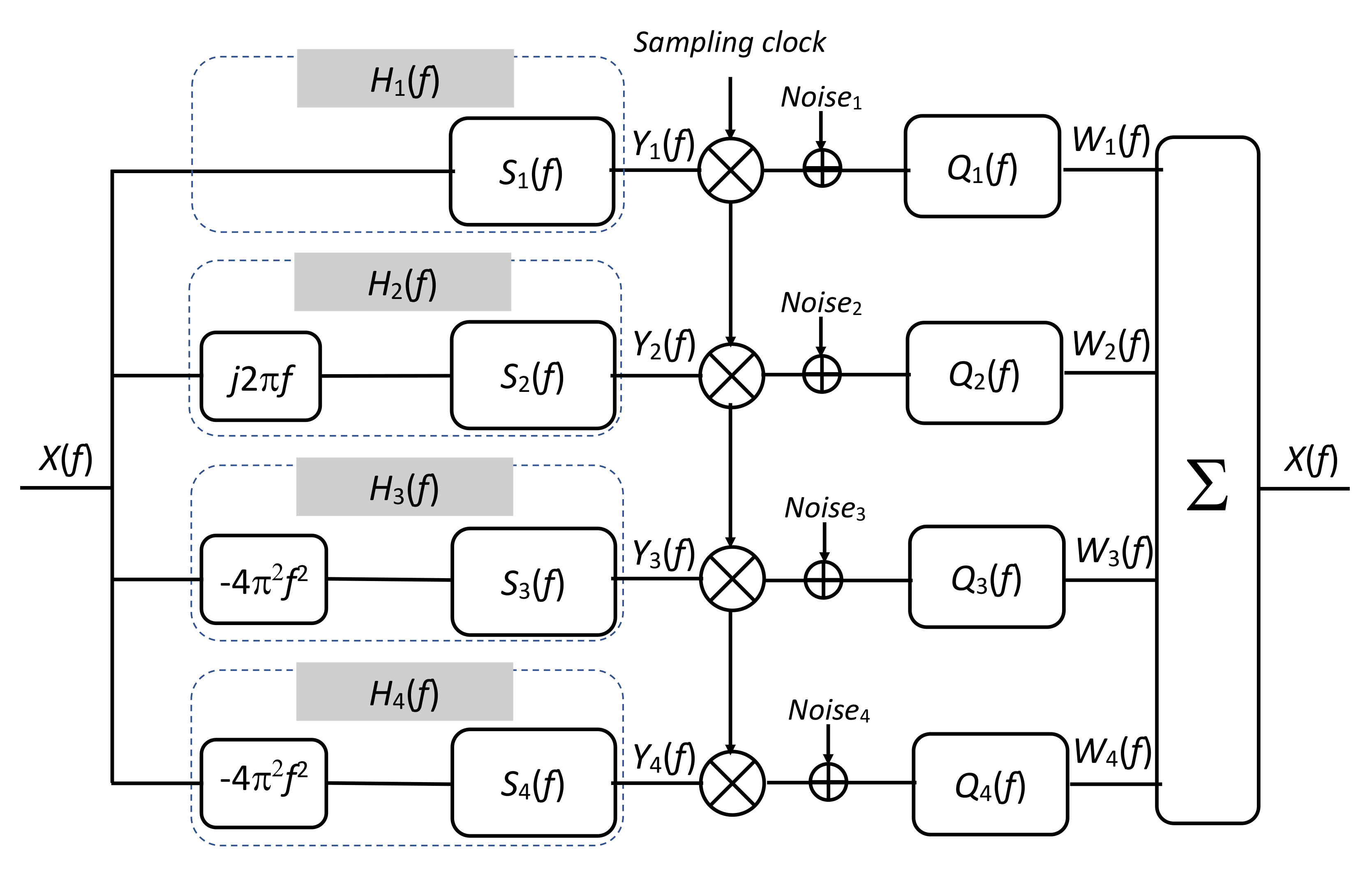
Figure 1 shows the block diagram of a four-channel system, where the input quantity is a position signal, and there are a velocity sensor and two acceleration sensors. The system is described using a frequency-domain representation, such that the well-known algebraic representations of the first-order and second-order time derivative operators (i.e., $j2\pi f$ and −$4{\pi }^2{f}^2$) are adopted. The frequency responses of the sensors and analog processing filters are $S_l\left(f\right)$ and $Q_l\left(f\right)$, l = 1, …, M, respectively, and the common input is $X\left(f\right)$. For each channel, a frequency response $H_l\left(f\right)$ can be defined, joining the frequency response of the operator with that of the serially connected sensor. The signals in input to the sampler can thus be described as $H_l\left(f\right)X\left(f\right)$, l = 1, …, M.

It is worth noticing that if the input signal is velocity or acceleration, one has to consider different block diagrams. In particular, if the velocity signal is chosen as the common input $X\left(f\right)$, then the position sensor will appear in the diagram after the algebraic operator $\frac{1}{j2\pi f}$ and the acceleration sensors after $j2\pi f$; if $X\left(f\right)$ represents instead the acceleration signal, then the position sensor will appear after −$\frac{1}{4{\pi }^2{f}^2}$, and the velocity sensor after $\frac{1}{j2\pi f}$.

2.3. Filter Identification

The proposed data fusion approach requires the identification of the frequency response of the filters, $Q_l\left(f\right)$, and the implementation of the corresponding discrete-time impulse responses, $q_l\left(n\right)$, which can be obtained by taking the inverse discrete Fourier transform of the $2L$-length sequence, $Q_l\left(k\right)$. The identification goal can be accomplished by exploiting the generalized sampling expansion theorem, according to which a band-limited signal $x\left(t\right)$, with single-sided bandwidth B, can be acquired by means of a linear multi-channel system with M independent channels operating at a rate not less than $f_s=\frac{2B}{M}$. Acquiring the signals means that a digital representation of the input characterized by a sample rate at least $M{f}_s=2B$ can be gained, without any loss of information, by combining the data streams from the independent channels.

It is worth noticing that the generalized sampling expansion allows the combination of the digital outputs of the individual sensors even when they, taken separately, operate below the Nyquist rate, provided that the overall number of samples per time unit from all the available sensors is not less than this. Thus, the individual sensors of the multi-channel architecture are allowed longer measurement time between one sample and the subsequent one, which can be exploited to improve the reading accuracy. Clearly, combining the output of all sensors provides a digital representation of the addressed kinematic quantity, which is characterized by a sample rate greater than or equal to the corresponding Nyquist rate. In detail, if a frequency-domain representation is adopted, one can state the identity:

$$X\left(f\right)=\frac{M}{f_s}\sum _{l=1}^M\sum _{k=-\infty }^{\infty }{H}_l\left(f-k\frac{f_s}{M}\right)X\left(f-k\frac{f_s}{M}\right)Q_l\left(f\right)$$

(3)

where $X\left(f\right)$ is the input signal; $H_l\left(f\right)$ and $Q_l\left(f\right)$ with $l=1,\dots ,M$ are the frequency responses of the channels and filters, respectively. Notice that sampling the output of the sensors $H_l\left(f\right)X\left(f\right)$ at a rate $\frac{f_s}{M}$ produces replication in the frequency domain at a pace $\frac{f_s}{M}$, as described by the infinite sum upon the index k.

This identity can be refined since the filters in (3) must have zero gain outside the bandwidth $(-B,B)$, because of the band-limitedness of the signal on the left side of the equation. This allows the inner sum to be limited to the terms picked by k ranging from $-M+1$ up to $M-1$.

Furthermore, due to the periodic structure of the argument of the sum, characterized by period $\frac{f_s}{M}$, the set of the $2M-1$ terms can be further divided into subsets that provide equation systems for the reconstruction filters that are valid on different portions of the interval $(-B,B)$. Specifically, if the interval $(-B,B)$ is partitioned into the M adjacent intervals $\left(-B+p\frac{f_s}{M},-B+(p+1)\frac{f_s}{M}\right)$ obtained for $p=0,\dots ,M-1$, and the characteristic function of each, namely ${\pi }_p\left(f\right)={\pi }_{\left(-B+p\frac{f_s}{M},-B+(p+1)\frac{f_s}{M}\right)}\left(f\right)$, which equals one in the subscript interval and zero outside, is used as a multiplying operator in Equation (3), one obtains:

$$X\left(f\right){\pi }_p\left(f\right)=\frac{M}{f_s}\sum _{k=p-(M-1)}^p\sum _{l=1}^M{H}_l\left(f-k\frac{f_s}{M}\right)Q_{lp}\left(f\right)X\left(f-k\frac{f_s}{M}\right)$$

(4)

where the function $Q_{lp}\left(f\right)$ provides the representation of the reconstruction filter $Q_l\left(f\right)$ valid in the p-th interval.

Equation (4) implies that, for any fixed p, and with k ranging from $p-(M-1)$ up to p,

$$\sum _{l=1}^M{H}_l\left(f-k\frac{f_s}{M}\right)Q_{lp}\left(f\right)=\frac{M}{f_s}{\pi }_p\left(f\right)\mathbf{\delta }\left(k\right)$$

(5)

where $\mathbf{\delta }\left(k\right)$ is the Kronecher delta function, equal to one for $k=0$ and zero for $k\ne 0$.

Equation (5) defines the functions $Q_{lp}\left(f\right)$, as solutions of the system:

$$\left[\begin{array}{ccc}{H}_1(f-(p-(M-1))\frac{f_s}{M})& \dots & H_M(f-(p-(M-1))\frac{f_s}{M})\\ ⋮& \ddots & ⋮\\ H_1(f-p\frac{f_s}{M})& \dots & H_M(f-p\frac{f_s}{M})\end{array}\right]\left[\begin{array}{c}{Q}_{1p}\left(f\right)\\ ⋮\\ Q_{Mp}\left(f\right)\end{array}\right]=\frac{M}{f_s}{\pi }_p\left(f\right){\mathbf{\delta }}_{M-p}$$

(6)

where ${\mathbf{\delta }}_{M-p}$ is a zero vector except in the $(M-p)$-th component equal to 1.

The system can be represented in a compact form as:

$${\mathbb{H}}_p{\mathbf{Q}}_p={\mathbf{\delta }}_{M-p}$$

(7)

where the bold character is used for the vector ${\mathbf{Q}}_p={(Q_{1p}\left(f\right),\dots ,Q_{Mp}\left(f\right))}^T$, and the blackboard bold character for the matrix, redefined as:

$${\mathbb{H}}_p={\pi }_p\left(f\right)\frac{f_s}{M}\left[\begin{array}{ccc}{H}_1(f-(p-(M-1))\frac{f_s}{M})& \dots & H_M(f-(p-(M-1))\frac{f_s}{M})\\ ⋮& \ddots & ⋮\\ H_1(f-p\frac{f_s}{M})& \dots & H_M(f-p\frac{f_s}{M})\end{array}\right]$$

(8)

In order to determine ${\mathbf{Q}}_p$, the determinant of the matrix in system (7) must be different from zero everywhere in the interval $(-B+p\frac{f_s}{M},-B+(p+1)\frac{f_s}{M})$. (It is so clarified in which sense the channels must be independent from each other as stated by the hypothesis of the theorem.)

Named ${\mathbb{G}}_p$, the inverse matrix of ${\mathbb{H}}_p$, i.e., ${\mathbb{G}}_p={\mathbb{H}}_p^{-1}$, the vector of the reconstruction filters for the p-th interval can be represented as:

$${\mathbf{Q}}_p={\mathbb{G}}_p{\mathbf{\delta }}_{M-p}$$

(9)

It is worth highlighting that the frequency-domain functions in matrix ${\mathbb{H}}_p$ are rightward shifted by $f_s$ upon any increment in p, namely ${\mathbb{H}}_p={\mathcal{T}}_{p{f}_s}[{\mathbb{H}}_0$], where ${\mathcal{T}}_{p{f}_s}$ represents the translation operator by $p{f}_s$. Since translation and matrix inversion commute between each other, it also holds that ${\mathbb{G}}_p={\mathcal{T}}_{p{f}_s}\left[{\mathbb{G}}_0\right]$. Thus, the vector of the reconstruction filters valid throughout the interval $(-B,B)$ can finally be gained by computing the elements of vector $\mathbf{Q}$ as:

$$\mathbf{Q}=\sum _{p=0}^{M-1}{\mathcal{T}}_{p{f}_S}\left[{\mathbb{G}}_0\right]{\mathbf{\delta }}_{M-p}$$

(10)

Hence, the time-domain representation of the signal, $x\left(t\right)$, can be gained by first filtering the sampled signals from each channel with the functions $q_l\left(t\right)$, corresponding to the inverse Fourier transformation of $Q_l\left(f\right)$, to obtain the signals $w_l\left(t\right)$, and then linearly combining all of them, in formulas:

$$\left\{\begin{array}{cc}{w}_l\left(t\right)\hfill & =\sum _{n=-\infty }^{+\infty }{y}_l\left(n{T}_s\right)q_l(t-n{T}_s)\hfill \\ x\left(t\right)\hfill & =c_l\sum _{l=1}^M{w}_l\left(t\right)\hfill \end{array}\right.$$

(11)

where, for instance, if all sensors are judged equally reliable and accurate, it can be chosen $c_l=\frac{1}{M}$, $l=1,\dots ,M$.

2.4. Filter Synthesis

The implementation of the proposed method requires the knowledge of the frequency responses of the sensors. From a practical point of view, the identification of each sensor is obtained in a laboratory through calibration tests that imply measuring the gain and phase delay characterizing the sensor at different frequencies. Specifically, a uniform grid with L frequencies, including the zero frequency and extending up to the bandwidth of the sensor, is considered. The measured gain and phase delay are then represented with a complex number with modulo equal to the gain and a negative angle equal to the phase delay. This sequence is prolonged by mirroring the measured sequence with complex conjugate values to form a $2L$-length sequence that satisfies Hermitian symmetry with respect to the L-th point. The $2L$-length sequence is finally interpreted as the discrete double-sided frequency response of the sensor. This sequence represents the input data required by the proposed method, i.e., the values $H_l\left({\nu }_k{f}_c\right)$, $l=1,\dots ,M$, where ${\nu }_k=\frac{k}{2L}$, $k=0,1,\dots ,2L-1$, and $f_c$ is the sample rate selected for the output result.

Using the values obtained through the identification procedure in the system of Equation (9), and solving the algebraic systems obtained for each frequency value ${\nu }_k{f}_c$, $k=0,1,\dots ,L$ allows us to determine the values of the double-sided frequency responses of the filters at the same frequencies, i.e., $Q_l\left({\nu }_k{f}_c\right)$. Taking the inverse discrete Fourier transform of the latter returns the coefficients of the finite impulse responses filters, $q_l\left(n\right)$, $n=0,1,\dots ,2L$, needed to perform the data fusion upon the output of the sensors, according to Equation (1).

The proposed method requires that sensors are synchronously clocked at the same sample rate $f_s$, which has to be no lower than $\frac{f_c}{M}$. If the adopted sample rate is $f_s=\frac{f_c}{K}$, with $K\le M$, the data streams from the individual sensors are first upsampled by K by interleaving $K-1$ zeros between any couples of subsequent samples and then filtered.

Concerning the choice of the filter length, some degrees of freedom are possible, taking into account that longer filters offer higher accuracy but longer transients.

3. Simulations

3.1. Performance Assessment

The proposed framework allows for the implementation of several methods, where the corresponding architectures can be differently configured in terms of number and type of adopted channels, redundancy level for each kinematic quantity, and length of the digital filters for the data fusion. Clearly, each method and corresponding architecture requires a dedicated analysis to assess the performance.

Here, one example related to a particular choice is discussed with the intent of highlighting how the main configuration parameters generally impact the performance. In detail, a four-channel architecture made up of one position sensor, one velocity sensor, and two redundant acceleration sensors is configured to accurately measure a position signal, as shown in Figure 1.

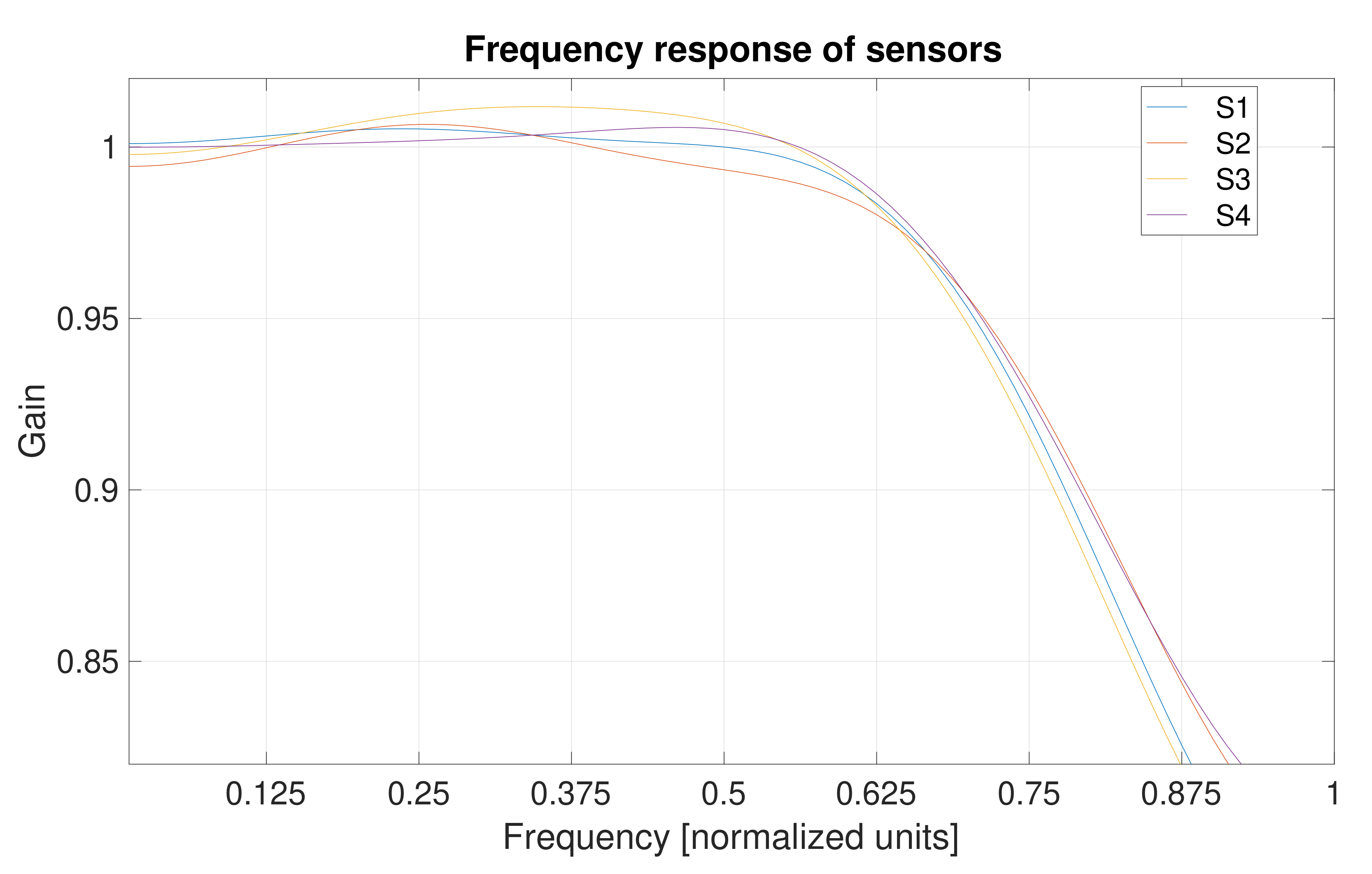
All sensors are characterized by a low-pass behavior, but their cut-off frequencies and in-band flatness are different from each other, as shown in Figure 2 and detailed in the corresponding caption. Frequency values are expressed in units normalized to the bandwidth of the system, and range from 0 up to 1.

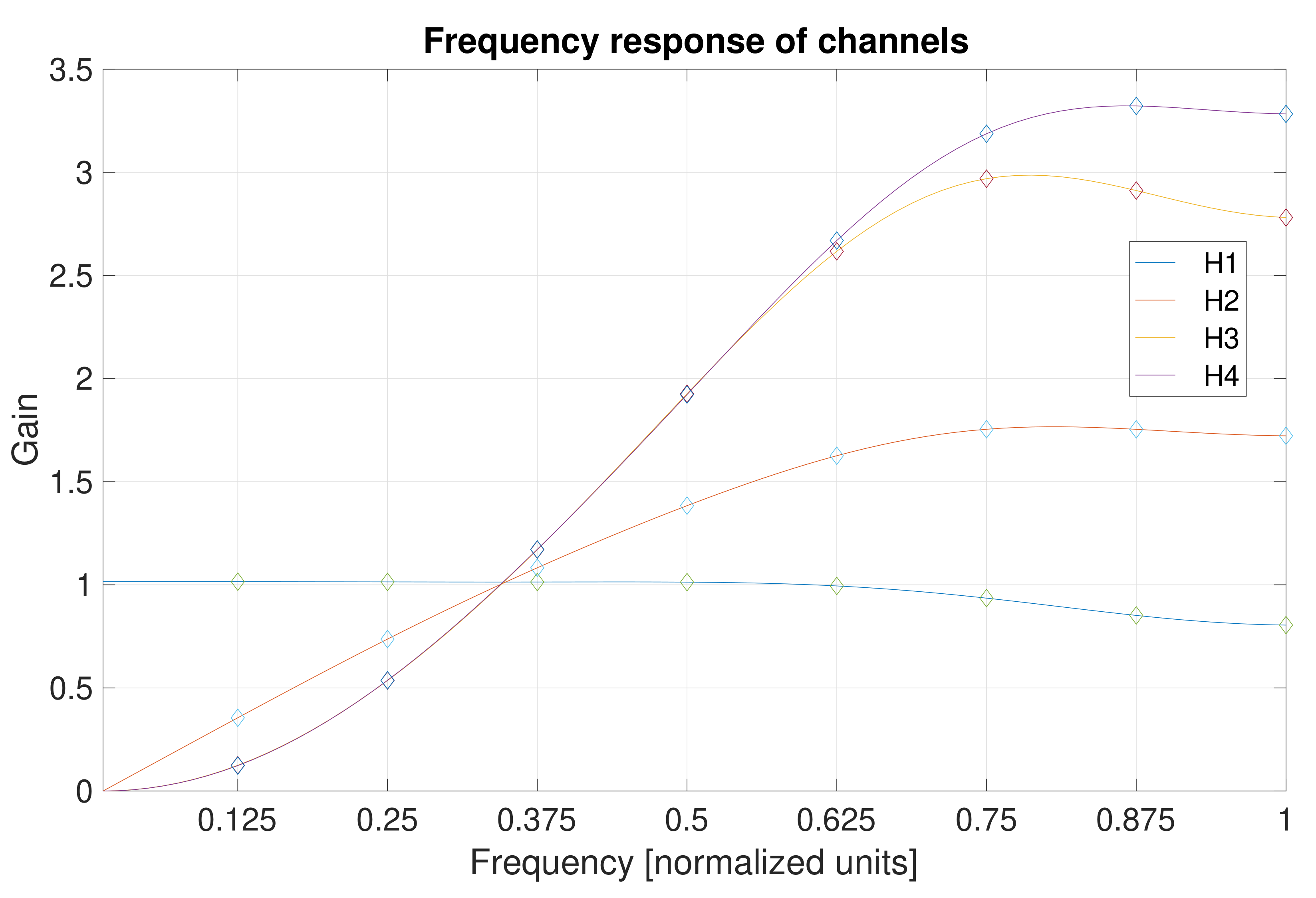
Coherently with the schematic in Figure 1, each channel is described in terms of a frequency response that includes the operator, inherent in the very nature of the sensor. Since, in the presence of redundant sensors, the independence of the channels could be not verified, the sampling operation of the channels, which are driven by clocks locked at the same frequency, is time-interleaved. The frequency responses of the simulated channels are given in Figure 3; the first- and second-order time derivatives are simulated by means of the first- and second-order finite forward differences.

The simulations assume that the frequency response of each channel can be determined on a uniform frequency grid, starting from the DC up to the nominal bandwidth of the channel, and that the collected data are affected by uncertainty on both magnitude and phase. The number of points forming the grid and the uncertainty affecting the values play an important role, because these data are the inputs needed for identifying the digital filters for the data fusion. In the simulated system, the values of the frequency response of any channels are characterized by 0.1% standard uncertainty for both magnitude and phase.

The set of digital filters needed to perform the data fusion is designed as illustrated in the theoretical framework presented in Section 2. The filters should ensure, for the whole system, a unitary gain, but a slight deviation between the actual gain and the target unitary value can hold due to the finite length of the adopted digital filters. This deviation is less significant for the frequency values corresponding to the points on the considered grid, where it is due to the sole uncertainty that characterizes the data collected at the identification stage, rather than for the frequency values that are amid these points.

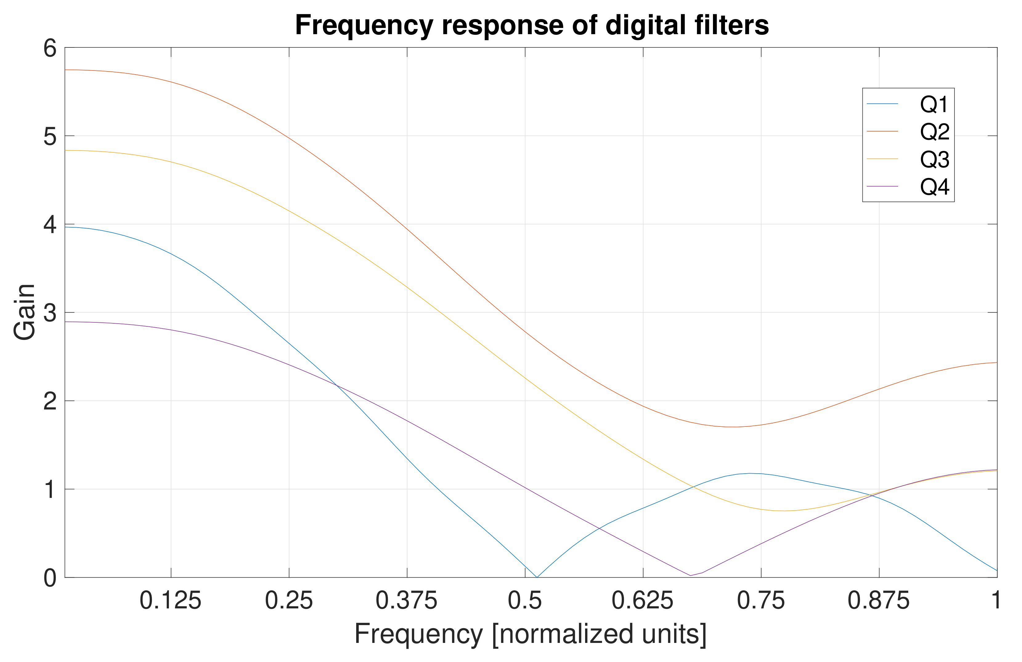
The four digital filters adopted by the simulations have $2L=16$ coefficients, and are designed taking into account the frequency response data obtained for eight equally spaced frequency points within the bandwidth of the channels; the frequency responses of the digital filters synthesized according to the proposed approach are shown in Figure 4.

The simulations have considered 200 sinusoidal inputs characterized by equally spaced values in the bandwidth of the system. For each sinusoidal input, 1000 realizations affected by broadband noise with a signal-to-noise ratio set at 20 dB are analyzed.

The accuracy of the system is evaluated using as a key performance index (KPI) the ratio between the mean square value of the input and the mean square value of the signal, obtained by taking the difference between the applied input and the output of the system.

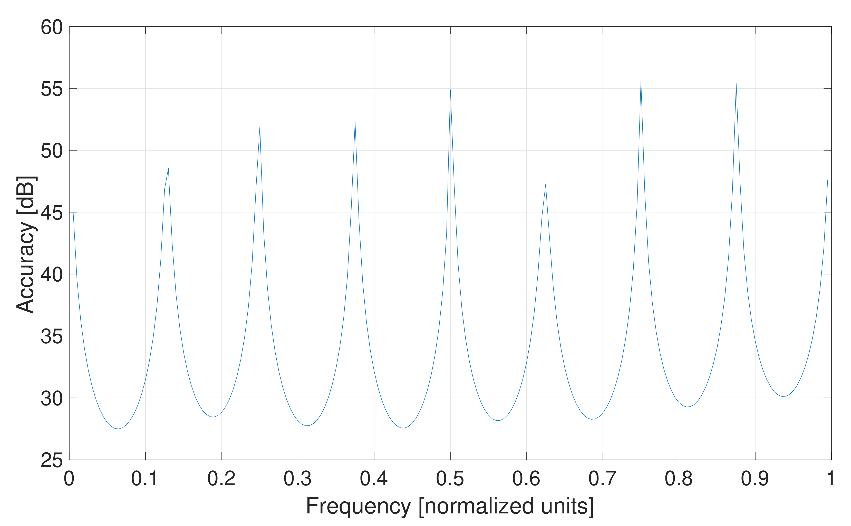
Figure 5 shows the mean value of the KPI, expressed in dB units, at the test frequencies. The obtained values are interpolated to have a continuous trace, in order to infer the accuracy of the system at frequencies that have not been directly measured. The accuracy of the position measurement provided by the data fusion approach is maximum, as expected, at the normalized frequency values corresponding to the points measured at the identification stage, which are characterized by the normalized frequency values $0.125k$, with $k=0,\dots ,7$. For such frequencies, the typical values of the KPI are greater than 45 dB, and are likely limited by the only measurement uncertainty of the data used at the filter design stage.

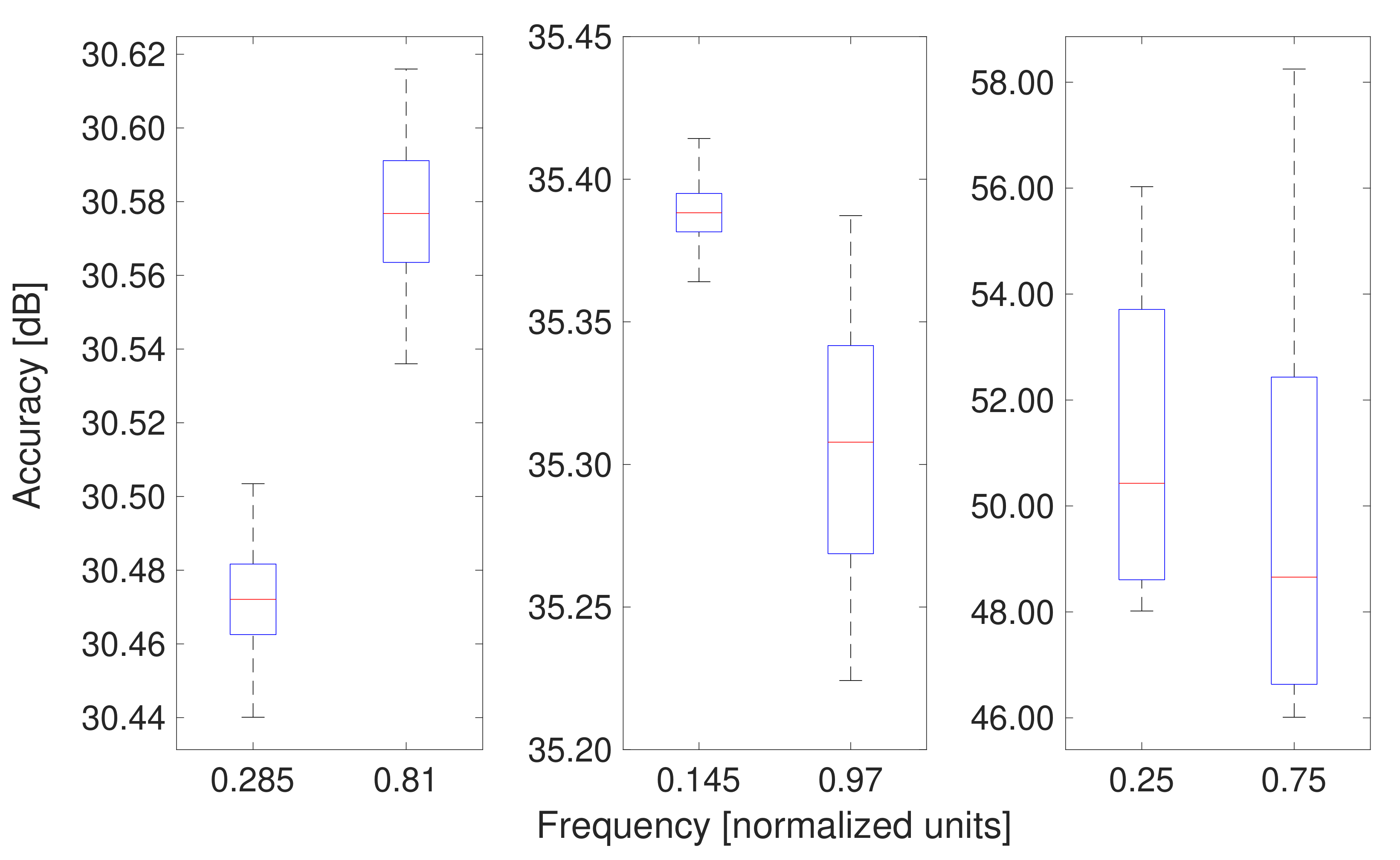
More details are given in Figure 6, where the results obtained for the KPI at a subset of the analyzed frequencies are summarized by means of boxplots, rather than compacted in a mean value as in Figure 5. In a boxplot, the central mark is the median, the edges of the box are the 25-th and 75-th percentiles, and the whiskers extend to the most extreme values considered to be not outliers. The frequencies are selected in order to show the results related to a couple of exemplars for the low performance (accuracy 30 dB), a couple for the intermediate performance (accuracy 35 dB), and a couple for the high performance (accuracy 45 dB). Low accuracy comes with less dispersion, while high accuracy comes with much dispersion. These effects are justified by the prevailing systematic error at frequencies far from the measured ones, and the rising relevance of the noise superimposed to the input as approaching high performance levels.

In the presence of non-sinusoidal test signals, such as pseudo-random trajectories, which have spectral contents uniformly spread throughout the bandwidth of the sensors, the typical accuracy offered by the method stands within the interval (33.9–36.2) dB with a mean at 35.0 dB; the evaluation has been carried out through Monte Carlo simulations based on 1000 pseudo-random trajectories. If the tests are repeated using the three-channel system obtained by excluding one of the acceleration sensors, the KPI estimates fall within the interval (31.6–33.8) dB and exhibit a mean value equal to 32.6 dB: the redundancy featuring the four-channel system allows an increment of 2.4 dB for the KPI.

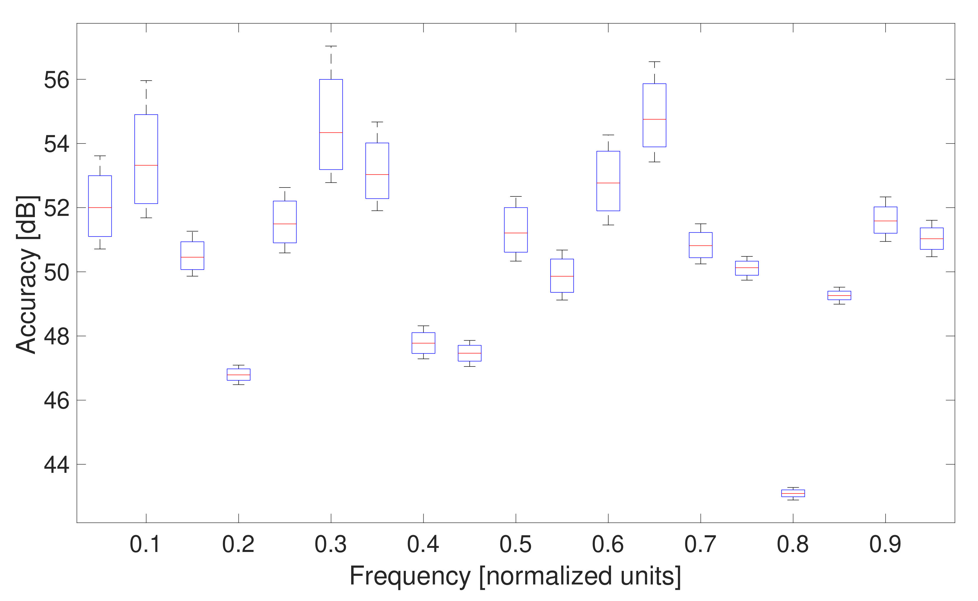
Intuitively, a finer knowledge of the frequency response of the channels, in terms of the number of measured values and related accuracy, allows the design of digital filters with more coefficients, which can grant higher accuracy. For instance, Figure 7 shows the boxplot (1000 realizations) for the accuracy at a subset of uniformly spaced frequencies, for a system that employs digital filters with 400 coefficients, the design of which has considered a set of 200 measurements characterized by 0.1% uncertainty for magnitude and phase: the results show that the accuracy generally improves throughout the bandwidth. Nevertheless, one has to take into account that a filter with L coefficients introduces a response delay equal to $L{T}_c$ seconds in the system, where $T_c$ is the sample period. The response delay limits the capability of the system in control applications, where the measurement of the kinematic quantities of a target must be obtained in a short time to correct the dynamic trajectory and minimize the fluctuation effects.

3.2. Comparison with a Benchmark

The proposed method for elaborating the output of the four sensors has been compared to a benchmark system that uses the same sensors. In the benchmark system, each sensor is complemented with a dedicated digital filter that assures a calibrated acquisition channel. Each digital filter is designed imposing a unitary gain at all measured frequency points, but, differently from the proposed method, the choice of its coefficients is independent of that of the other sensors in the same architecture.

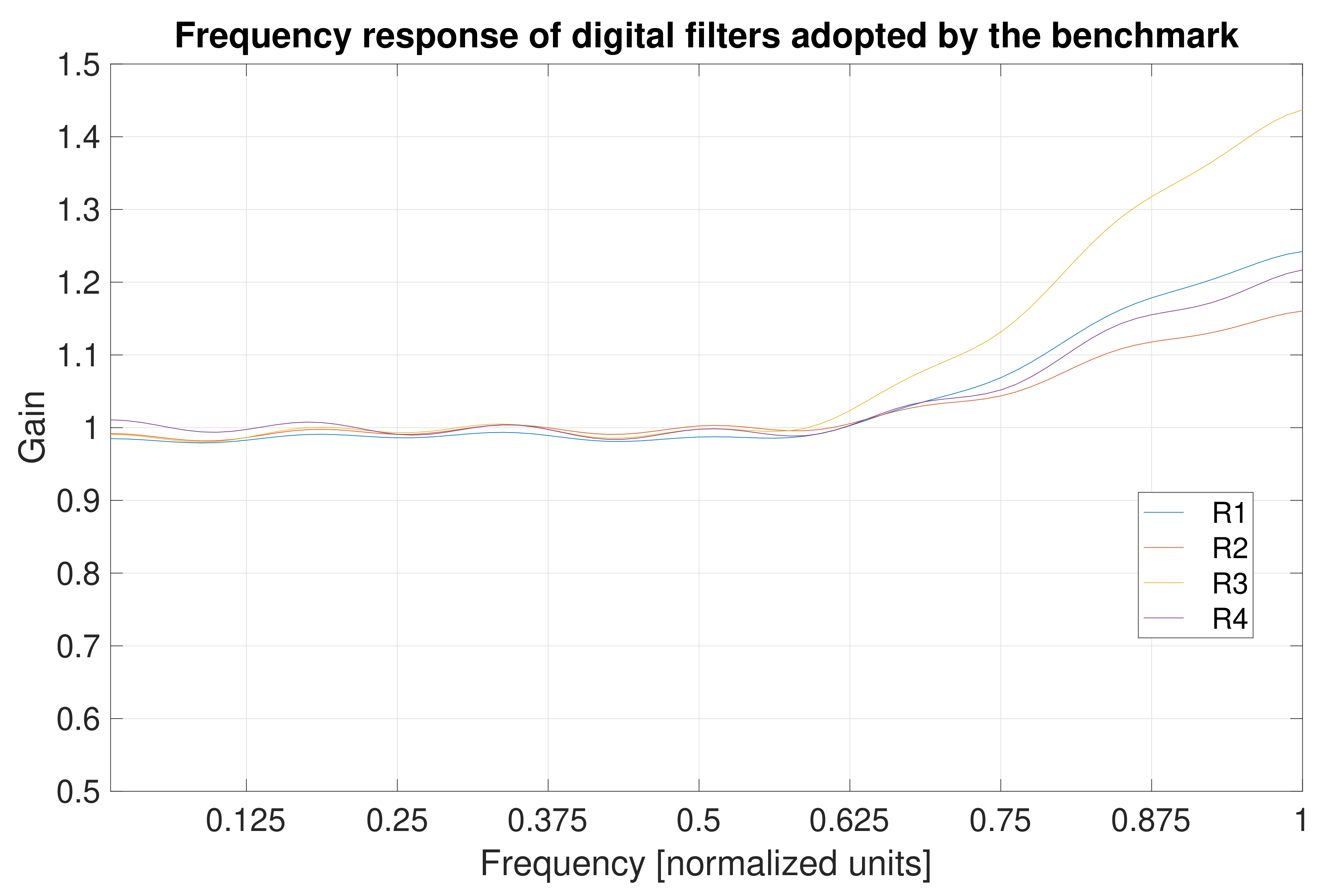
It is assumed that at the identification stage, the frequency response of the sensors can be measured with the same uncertainty level used to evaluate the proposed system, i.e., 0.1% for both magnitude and phase. For an equal comparison, the length of the digital filters of the benchmark system is chosen equal to $2L=16$, namely that chosen for the proposed system. Notice, however, that the digital filters aimed at the calibration (i.e., equalization) of the individual channels are evidently different from those used by the proposed method, even if they are designed using the same input data, as shown in Figure 8.

The outputs of the channels of the benchmark system are further elaborated in the case of velocity and acceleration signals to obtain position signals. To this end, velocity and acceleration signals are digitally integrated once and twice, respectively; the digital integration is obtained through the cumulative sum. The four position signals are combined to obtain a single representative position signal, which is compared to that offered by the proposed system.

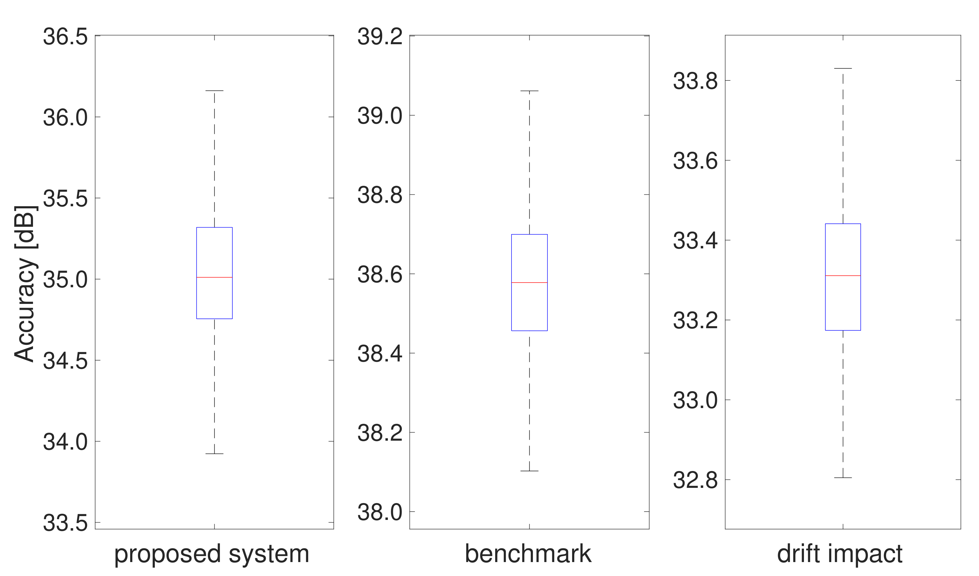
Pseudo-random trajectories that have spectral contents uniformly spread throughout the bandwidth of the sensors are used as test signals. Figure 9 shows the accuracy information for the proposed method and the considered benchmark, both summarized by means of boxplots evaluated on 1000 pseudo-random trajectories. As stated, the accuracy of the proposed method is within the interval (33.9–36.2) dB and typically sets at 35.0 dB, whereas that of the benchmark is within the interval (38.1–39.1) dB and typically sets at 38.6 dB.

The benchmark system provides a theoretical limit, which is difficult, if not impossible, to achieve when stepping from simulation, where several effects can be easily controlled and neutralized, to practice.

The benchmark, as well as all the systems that have to evaluate the integral of a signal, have a weak point, which consists in the use of algorithms, such as the cumulative sum, that act as unstable auto-regressive filters. These algorithms typically produce divergent outputs in the presence of offsets at the input stage.

Steady or wandering offsets are very common and difficult to compensate for in kinematic sensors. At the calibration stage, it is very difficult to directly measure weak offsets that can be smaller than the resolution of the adopted meter. However, in a digital system that uses a cumulative sum, for a run that considers N consecutive samples, the offset produces a drift that reaches a peak value equal to N times the offset amount (linear drift), and a peak value equal to $\frac{1}{2}N(N+1)$ (quadratic drift) for the same run if the cumulative sum is repeated twice.

To provide evidence of the issue, Figure 10 shows the position of a target that oscillates with respect to a rest position, as measured both by a dedicated displacement sensor and by integrating twice the output of an acceleration sensor affected by an offset equal to 1 ppm the output range of the sensor. A red trace shows the parabolic drift due to the offset, which makes the latter position measurement progressively deviate from that offered by the dedicated sensor.

The offset can be estimated by dividing the peak deviation between the signal and the reference by the aforementioned quadratic factor. Unfortunately, static compensation is never perfect and offset residuals can show up, especially if the offset is not constant in time. The effect of a residual or unstable offset still becomes manifest as linear drift in the case of velocity sensors, and parabolic drift in the case of acceleration sensors.

As discussed in the Introduction, drifts can be counteracted dynamically, if one can rely on a reliable and accurate position sensor, which does not undergo any drift. Dynamic compensation is performed seamlessly during the operation of the system, and it is repeated at a given cadence to indicate that the performance of the multi-sensor system degrades beneath an acceptance level. The choice of the duration of the time interval between the compensation actions is bounded by a trade-off: short intervals allow frequent but less effective compensation; long intervals are the basis for accurate estimations, but expose the system to poor tracking capabilities, giving the drift more time to exert its effect.

To evaluate the impact of the offset on the accuracy of both multi-sensor systems, namely the proposed one and the benchmark, the results of further simulations performed in the presence of an offset at the output of the acceleration sensors are discussed. In particular, a steady offset equal to 1 ppm (relative to the output range of the acceleration sensor) is simulated. The dynamic compensation is performed any $N=100$ samples (i.e., any 10 ms for a 10 kHz sample rate) such that the quadratic drift can reach at most a deviation equal to 0.5% the output range of the sensor, which is just detectable since it is at the level of the typical output noise. In this case, the accuracy of the benchmark degrades to values in the interval (32.8–33.8) dB, as reported in Figure 9.

It is worth noticing that, conversely, the proposed system adopts an inherent solution to extract position information from velocity and acceleration signals without using cumulative sums. More specifically, it uses finite impulse response filters, which are stable filters that confer finite gain to zero and low frequencies (see the frequency responses of the digital filters in Figure 4), where the spectral contents of the offset reside. The impact on the accuracy of an offset equal to 1 ppm in the output range of the sensor is therefore not appreciable on the proposed system, which confirms the results shown in Figure 9.

4. Conclusions

A class of multi-sensor data fusion methods for kinematic quantities has been proposed. All the methods are based on the same general framework and can be distinguished between each other according to the number and types of available kinematic sensors. The methods enable the exploitation of the redundancy of homogeneous kinematic sensors and, more generally, of the combination of the outputs offered by heterogeneous kinematic sensors.

The study has analyzed the possibilities of one of these methods in its basic implementation, and has carried out a fair comparison with the most immediate competing method that one can consider to perform data fusion. In particular, it has been highlighted that, for both the proposed method and the benchmark, there are plenty of possibilities for performance improvements—for example, by exploiting the optimization techniques for advanced digital filter design. However, it should be underlined that optimization was beyond the scope of this study, which focused on defining a general framework, rather than a specific method and corresponding implementation. The considered four-channel architecture, as stated in Section 3, has been used only with the intent of highlighting how the main configuration parameters generally impact the performance of a method born from the proposed framework.

The most interesting feature of the methods consists in their robustness with respect to the undesired effects due to offsets and/or flicker and random walk noise. The offset error that affects the majority of the systems entirely based on micro-machined electro-mechanical systems is, in fact, avoided by using FIR filters, characterized by a finite gain at low frequency. Differently, the solutions that exploit (explicitly or implicitly) the time-integration processing to obtain position measurements from velocity and/or acceleration signals are at risk of poor accuracy even in the presence of a high level of redundancy, since even weak offsets can produce relevant errors due to their cumulative effects.

It can be concluded that the class of methods generated by the proposed framework proficiently combine direct position, velocity, and acceleration measurements. In particular, this is effective any time the position signal is characterized by coarse precision, and the velocity and acceleration signals are affected by issues due to offset, flicker, or random walk noise. In these scenarios, the methods of the considered class allow one to benefit from the presence of the heterogeneous sensors, which enable the position measurement with drift-free tributaries.

References

- Samatas, G.G.; Pachidis, T.P. Inertial Measurement Units (IMUs) in Mobile Robots over the Last Five Years: A Review. Designs 2022, 6, 17. [Google Scholar] [CrossRef]
- Viana, K.; Zubizarreta, A.; Diez, M. A Reconfigurable Framework for Vehicle Localization in Urban Areas. Sensors 2022, 22, 2595. [Google Scholar] [CrossRef] [PubMed]
- Sarker, A.; Emenonye, D.R.; Kelliher, A.; Rikakis, T.; Buehrer, R.M.; Asbeck, A.T. Capturing Upper Body Kinematics and Localization with Low-Cost Sensors for Rehabilitation Applications. Sensors 2022, 22, 2300. [Google Scholar] [CrossRef] [PubMed]
- Seco, T.; Lázaro, M.T.; Espelosín, J.; Montano, L.; Villarroel, J.L. Robot Localization in Tunnels: Combining Discrete Features in a Pose Graph Framework. Sensors 2022, 22, 1390. [Google Scholar] [CrossRef]
- Uradziński, M.; Mieczysław, B. Assessment of static positioning accuracy using low-cost smartphone GPS devices for geodetic survey points’ determination and monitoring. Appl. Sci. 2020, 10, 5308. [Google Scholar] [CrossRef]
- He, X.; Gao, W.; Sheng, C.; Zhang, Z.; Pan, S.; Duan, L.; Zhang, H.; Lu, X. LLiDAR-Visual-Inertial Odometry Based on Optimized Visual Point-Line Features. Remote Sens. 2022, 14, 622. [Google Scholar] [CrossRef]
- Barbosa, L.A.; Costa, D.C.; de Oliveira, H.C. Evaluation of low-cost GNSS receivers for speed monitoring. Case Stud. Transp. Policy 2022, 10, 1. [Google Scholar] [CrossRef]
- Zhang, F.; Wang, Z.; Zhong, Y.; Chen, L. Localization Error Modeling for Autonomous Driving in GPS Denied Environment. Electronics 2022, 11, 647. [Google Scholar] [CrossRef]
- Ai, X.; Zheng, Y.; Xu, Z.; Zhao, F. Parameter Estimation for Uniformly Accelerating Moving Target in the Forward Scatter Radar Network. Remote Sens. 2022, 14, 1006. [Google Scholar] [CrossRef]
- Vargas, J.; Alsweiss, S.; Toker, O.; Razdan, R.; Santos, J. An overview of autonomous vehicles sensors and their vulnerability to weather conditions. Remote Sens. 2021, 21, 5397. [Google Scholar] [CrossRef]
- Pirník, R.; Hruboš, M.; Nemec, D.; Mravec, T.; Božek, P. Integration of inertial sensor data into control of the mobile platform. In Federated Conference on Software Development and Object Technologies; Springer: Cham, Switzerland, 2015. [Google Scholar]
- Narasimhappa, M.; Mahindrakar, A.D.; Guizilini, V.C.; Terra, M.H.; Sabat, S.L. MEMS-based IMU drift minimization: Sage Husa adaptive robust Kalman filtering. IEEE Sens. J. 2019, 20, 250–260. [Google Scholar] [CrossRef]
- Brossard, M.; Bonnabel, S. Learning wheel odometry and IMU errors for localization. In Proceedings of the 2019 International Conference on Robotics and Automation (ICRA), Montreal, QC, Canada, 20–24 May 2019. [Google Scholar]
- Wen, Z.; Yang, G.; Cai, Q. An Improved Calibration Method for the IMU Biases Utilizing KF-Based AdaGrad Algorithm. Sensors 2021, 21, 5055. [Google Scholar] [CrossRef] [PubMed]
- Cui, H.; Guan, Y.; Chen, H. Rolling element fault diagnosis based on VMD and sensitivity MCKD. IEEE Access 2021, 9, 120297–120308. [Google Scholar] [CrossRef]
- Zhang, Z.H.; Min, F.; Chen, G.S.; Shen, S.P.; Wen, Z.C.; Zhou, X.B. Tri-Partition State Alphabet-Based Sequential Pattern for Multivariate Time Series. Cogn. Comput. 2021, 11, 11294. [Google Scholar] [CrossRef]
- Deng, W.; Li, Z.; Li, X.; Chen, H.; Zhao, H. Compound fault diagnosis using optimized MCKD and sparse representation for rolling bearings. IEEE Trans. Instrum. Meas. 2022, 71, 3508509. [Google Scholar] [CrossRef]
- Li, S.; Gao, Y.; Meng, G.; Wang, G.; Guan, L. Accelerometer-Based Gyroscope Drift Compensation Approach in a Dual-Axial Stabilization Platform. Electronics 2019, 8, 594. [Google Scholar] [CrossRef] [Green Version]
- Poulose, A.; Eyobu, O.S.; Han, D.S. An indoor position-estimation algorithm using smartphone IMU sensor data. IEEE Access 2019, 7, 11165–11177. [Google Scholar] [CrossRef]
- Lahat, D.; Adali, T.; Jutten, C. Multimodal Data Fusion: An Overview of Methods, Challenges, and Prospects. Proc. IEEE-Invit. Pap. 2015, 103, 1449–1477. [Google Scholar] [CrossRef] [Green Version]
- Macii, D.; Boni, A.; De Cecco, M.; Petri, D. Tutorial 14: Multisensor Data—Part 14 in a series of tutorials in instrumentation and measurement. IEEE Instrum. Meas. Mag. 2008, 6, 24–33. [Google Scholar] [CrossRef]
- Liu, Z.; Xiao, G.; Liu, H.; Wei, H. Multi-Sensor Measurement and Data Fusion. IEEE Instrum. Meas. Mag. 2020, 2, 28–36. [Google Scholar] [CrossRef]
- D’Adamo, T.; Phillips, T.; McAree, P. LiDAR-Stabilised GNSS-IMU Platform Pose Tracking. Sensors 2022, 22, 2248. [Google Scholar] [CrossRef] [PubMed]
- Ravindran, R.; Santora, M.J.; Jamali, M.M. Camera, LiDAR, and Radar Sensor Fusion Based on Bayesian Neural Network (CLR-BNN). IEEE Sens. J. 2022, 22, 6964–6974. [Google Scholar] [CrossRef]
- Monrroy Cano, A.; Lambert, J.; Edahiro, M.; Kato, S. Single-Shot Intrinsic Calibration for Autonomous Driving Applications. Sensors 2022, 22, 2067. [Google Scholar] [CrossRef] [PubMed]
- Qiu, Z.; Zhang, J.; Lyu, S. Compensation Filtering for Spacecraft Attitude Estimation Using Error-Covariance Reconstruction. IEEE Trans. Instrum. Meas. 2022. [Google Scholar] [CrossRef]
- Dong, X.; Huang, Y.; Lai, P.; Huang, Q.; Su, W.; Li, S.; Xu, W. Research on Decomposition of Offset in MEMS Capacitive Accelerometer. Micromachines 2021, 12, 1000. [Google Scholar] [CrossRef]
- Li, Q.; Nevalainen, P.; Peña Queralta, J.; Heikkonen, J.; Westerlund, T. Localization in Unstructured Environments: Towards Autonomous Robots in Forests with Delaunay Triangulation. Remote Sens. 2020, 12, 1870. [Google Scholar] [CrossRef]
- Mikov, A.; Panyov, A.; Kosyanchuk, V.; Prikhodko, I. Sensor Fusion For Land Vehicle Localization Using Inertial MEMS and Odometry. In Proceedings of the 2019 IEEE International Symposium on Inertial Sensors and Systems (INERTIAL), Naples, FL, USA, 1–5 April 2019; pp. 1–2. [Google Scholar] [CrossRef]
- De Alteriis, G.; Accardo, D.; Conte, C.; Schiano Lo Moriello, R. Performance Enhancement of Consumer-Grade MEMS Sensors through Geometrical Redundancy. Sensors 2021, 21, 4851. [Google Scholar] [CrossRef]
- Larey, A.; Aknin, E.; Klein, I. Multiple Inertial Measurement Units–An Empirical Study. IEEE Access 2020, 8, 75656–75665. [Google Scholar] [CrossRef]
- Han, J.-H.; Park, C.-H.; Kwon, J.H.; Lee, J.; Kim, T.S.; Jang, Y.Y. Performance Evaluation of Autonomous Driving Control Algorithm for a Crawler-Type Agricultural Vehicle Based on Low-Cost Multi-Sensor Fusion Positioning. Appl. Sci. 2020, 10, 4667. [Google Scholar] [CrossRef]
- Kassas, Z.Z.; Maaref, M.; Morales, J.J.; Khalife, J.J.; Shamei, K. Robust vehicular localization and map matching in urban environments through IMU, GNSS, and cellular signals. IEEE Intell. Transp. Syst. Mag. 2020, 12, 36–52. [Google Scholar] [CrossRef]
- Yang, P.; Duan, D.; Chen, C.; Cheng, X.; Yang, L. Multi-sensor multi-vehicle (msmv) localization and mobility tracking for autonomous driving. IEEE Trans. Veh. Technol. 2020, 69, 14355–14364. [Google Scholar] [CrossRef]
- Gao, B.; Hu, G.; Gao, S.; Zhong, Y.; Gu, C. Multi-Sensor Optimal Data Fusion Based on the Adaptive Fading Unscented Kalman Filter. Sensors 2018, 18, 488. [Google Scholar] [CrossRef] [PubMed] [Green Version]
- Lu, Y.; Ma, H.; Smart, E.; Yu, H. Real-Time Performance-Focused Localization Techniques for Autonomous Vehicle: A Review. IEEE Trans. Intell. Transp. Syst. 2021. [Google Scholar] [CrossRef]
- Fayyad, J.; Jaradat, M.A.; Gruyer, D.; Najjaran, H. Deep Learning Sensor Fusion for Autonomous Vehicle Perception and Localization: A Review. Sensors 2020, 20, 4220. [Google Scholar] [CrossRef]
- Liu, J.; Guo, G. Vehicle localization during GPS outages with extended Kalman filter and deep learning. IEEE Trans. Instrum. Meas. 2021, 70, 1–10. [Google Scholar] [CrossRef]
- Papoulis, A. Generalized sampling expansion. IEEE Trans. Circuits Syst. 1977, 24, 652–654. [Google Scholar] [CrossRef]
Figure 1.
Diagram of a multi-channel system with 4 sensors. The input quantity is a position signal, and there are a velocity sensor and 2 acceleration sensors, characterized in terms of their frequency responses . The operators and − stand at the front-end of the velocity and acceleration sensors to transform the position input into velocity and acceleration signals. The common input is and represents the spectrum of a position signal; each channel is described in terms of a frequency response . The outputs of the sensors are sampled and degraded by (quantization) noise before entering the filters required to combine the outputs of the individual channels.
Figure 2.
Amplitude frequency response of the adopted sensors; the values of the frequency are expressed in units normalized to the bandwidth of the system, and range from 0 up to 1. All responses are characterized by 3 dB cut-off normalized frequencies that fall in the interval (0.93–0.97) with a 95% confidence level; all frequency responses grant flatness within 0.18 dB up to 0.625 normalized frequency.
Figure 3.
The amplitude frequency response of the 4 channels highlights the behavior of the channel hosting the position sensor (blue), the velocity sensor (red), and the acceleration sensors (yellow and magenta) within the input bandwidth. The diamond markers highlight the points considered at the identification stage.
Figure 4.
Frequency responses of the 4 digital filters that are used to perform the data fusion. All filters are characterized by coefficients.
Figure 5.
Accuracy is expressed in terms of a KPI defined as the mean value of the ratio, given in dB unit, between the mean square value of the input and the mean square value of the signal, obtained by taking the difference between the applied input and the output of the system. The values are interpolated to have a continuous trace, in order to infer the accuracy of the system at frequencies that have not been directly measured.
Figure 6.
Boxplots for the KPI utilized to evaluate the accuracy of the proposed data fusion method. The values are related to a selection of the test frequencies to highlight how the dispersion of the KPI changes at different performance levels.
Figure 7.
Boxplots for the KPI evaluated at normalized frequencies uniformly spaced by 0.05 units when the digital filters are characterized by length = 400.
Figure 8.
Frequency response of the digital filters adopted by the benchmark system to perform the equalization of the sensors. The frequency responses are evidently different from those used by the proposed method given in Figure 4.
Figure 9.
Accuracy offered by the proposed system (33.9–36.2) dB and the considered benchmark, both in ideal conditions (38.1–39.1) dB and in the presence of a constant offset equal to 1 ppm (relative to the output range of the accelerometer). The results are summarized by means of boxplots evaluated on 1000 tests performed on pseudo-random trajectories.
Figure 10.
Displacement of a target around its rest position. The oscillations are simulated with a multi-frequency signal that is characterized by a peak value equal to 0.9 m, and 3 components at normalized frequencies equal to 0.0071, 0.0272, and 0.0146. The blue trace represents the output of the displacement sensor; the black trace is obtained by integrating the output of the acceleration sensor affected by an offset equal to 1 ppm (relative to the output range of the sensor); the red trace highlights the quadratic drift corresponding to the difference between the signals.
Publisher’s Note: MDPI stays neutral with regard to jurisdictional claims in published maps and institutional affiliations. |
© 2022 by the authors. Licensee MDPI, Basel, Switzerland. This article is an open access article distributed under the terms and conditions of the Creative Commons Attribution (CC BY) license (https://creativecommons.org/licenses/by/4.0/).
Share and Cite
MDPI and ACS Style
D’Arco, M.; Guerritore, M. Multi-Sensor Data Fusion Approach for Kinematic Quantities. Energies 2022, 15, 2916. https://doi.org/10.3390/en15082916
AMA Style
D’Arco M, Guerritore M. Multi-Sensor Data Fusion Approach for Kinematic Quantities. Energies. 2022; 15(8):2916. https://doi.org/10.3390/en15082916
Chicago/Turabian StyleD’Arco, Mauro, and Martina Guerritore. 2022. "Multi-Sensor Data Fusion Approach for Kinematic Quantities" Energies 15, no. 8: 2916. https://doi.org/10.3390/en15082916
Note that from the first issue of 2016, this journal uses article numbers instead of page numbers. See further details here.