Latent-Space Dynamics for Prediction and Fault Detection in Geothermal Power Plant Operations

Abstract

This paper presents a latent-space dynamic neural network (LSDNN) model for the multi-step-ahead prediction and fault detection of a geothermal power plant’s operation. The model was trained to learn the dynamics of the power generation process from multivariate time-series data and the effects of exogenous variables, such as control adjustment and ambient temperature. In the LSDNN model, an encoder–decoder architecture was designed to capture cross-correlation among different measured variables. In addition, a latent space dynamic structure was proposed to propagate the dynamics in the latent space to enable prediction. The prediction power of the LSDNN was utilized for monitoring a geothermal power plant and detecting abnormal events. The model was integrated with principal component analysis (PCA)-based process monitoring techniques to develop a fault-detection procedure. The performance of the proposed LSDNN model and fault detection approach was demonstrated using field data collected from a geothermal power plant.

1. Introduction

As transitions from fossil fuel-dependent to renewable sources of energy gain traction, technologies are being developed to improve the efficiency of energy production by geothermal power plants [1]. With the increase in the utilization of geothermal energy, it is projected that, by 2050, geothermal power plants will generate 8.3% of the world’s power and will serve 17% of the world population [2]. Geothermal power plants recover heat energy from hot underground rocks and convert it to electrical energy. The reliability and efficiency of operating geothermal power plants can be improved by optimizing the design of the power plants and by monitoring and controlling their operations. Modeling and predicting a power plant’s performance under different operating conditions are important enabling tools for controlling and optimizing power plant design and operations. Physics-based simulation models have traditionally been used to model the dynamics of geothermal power plants [3,4]. However, these models are typically complex to construct, since significant efforts and in-depth knowledge and expertise are required to model the behavior of the underlying components and their interactions accurately [5]. In addition, since the configurations and characteristics of geothermal power plants depend on the field conditions and performance requirements [6], many uncertain parameters are involved when building simulation models for different power plants.

A good alternative to physics-based simulation models is data-driven modeling, where the model is trained using existing monitoring and performance data to learn the statistical patterns and relationships among different components to predict their future behavior and performance. Recently, the success of deep learning has renewed interest in the use of artificial neural networks (ANN) as data-driven proxy models for prediction in physical systems. Various neural network architectures have been applied to model and predict the performance of different energy systems. Multilayer perceptron (MLP) is used to forecast the output power of a photovoltaic plant based on 48 h ahead weather forecasts [7]. The autoencoder structure has been combined with Long Short-Term Memory (LSTM) to forecast the energy output of 21 solar power plants [8]. To model a large-scale supercritical boiler plant, individual recurrent neural network (RNN) models have been built for different subsystems and combined based on the subsystems’ input and output relationships [9]. Convolutional neural networks (CNNs) that offer significant efficiency in processing images have also been applied to two-channel two-dimensional images containing information related to the states and changes of states in a nuclear power plant for the classification of abnormal events [10]. In the geothermal domain, MLP has been used to aid the design and optimization of binary geothermal power plants by predicting the generated power of the system and the required circulation pump power [11]. In addition, a deep neural network model has been used to predict geothermal reservoir temperatures based on hydrogeochemical parameters [12]. In [13], LSTM and MLP were used to predict the productivity of a multilateral-well geothermal system, where the LSTM was used to learn the trend in historical productions, and the MLP was used to make predictions based on the output of the LSTM and the constraints of reservoir properties.

Although there have been many applications of ANN related to geothermal power generation, they mainly focused on subsurface processes. For the data modeling of geothermal power plants, studies were focused on the steady-state surface processes. The drawback of steady-state modeling is that it fails to capture the autocorrelation in time-series data and the dynamics of the power generation process affected by ambient disturbances and control adjustments. In addition, the underlying physics in the power generation process serve as a constraint that relates measured quantities, such as temperature and pressure. As a result, the existing relationships in the data imply that the main variations can be captured and represented in a low-dimensional latent space. To achieve latent representation, the autoencoder (AE) structure has been used for applications, such as dimensionality reduction [14] and system identification [15]. To capture the autocorrelations in the data and to describe the nonlinear dynamics of a system, neural networks with a single hidden layer have been used [16]. In addition, recurrent neural networks that use nonlinear autoregressive model with exogenous inputs (NARX) have been implemented with a multilayer perceptron. It was shown that the resulting network is often better at discovering long-term dependencies than conventional recurrent neural networks, mainly due to the delays in the network acting as jump-ahead connections during training [17]. In [18], the authors showed that, by using output feedback, the NARX neural network was able to predict complex time series.

In geothermal power plants, faults, such as working fluid leakage, ingress of non-condensable gases into working gas, and production pump failure, can lead to poor performance or even catastrophic failure. Due to the time scale of the faults, some of them are difficult to be spotted by the plant operators. In these cases, statistical process monitoring (SPM) techniques can help by constantly monitoring data. SPM has been used in many industrial processes, such as chemicals and semiconductor manufacturing [19], but it has not been used for applications related to geothermal power generation. Fault detection is an essential part of SPM. It is used to detect abnormal events within the process, which is crucial for maintaining normal operating conditions and preventing catastrophic failures. Principal component analysis (PCA) has been widely used for static process monitoring [19,20,21]. However, as PCA assumes that the data samples are independent in time, directly applying PCA-based monitoring techniques to time-series data may lead to poor fault detection results due to the presence of autocorrelation. To deal with this issue, fault-detection procedures were proposed in [22,23], in which the authors first extracted the dynamics from multivariate time-series data, which removed the autocorrelations within the data. As a result, the residuals only contain static variations, which can be modeled using the PCA and lend themselves to detect faults.

In this paper, we present a novel latent-space dynamic neural network (LSDNN) architecture to exploit the characteristics of the data collected from geothermal power plants. The LSDNN model combines the advantages of autoencoder structure and the NARX neural network model to effectively capture the cross-correlation and autocorrelation from multivariate time-series measurements. The dynamic model was trained to learn the interactions and statistical relationships between different measured and exogenous variables in the power generation process. The trained neural network was then used to make multi-step-ahead predictions about the performance of each component in the power plant. Furthermore, the predictions were used to formulate a fault detection algorithm for the plant, where the autocorrelations were first removed through prediction, and static process monitoring techniques were applied to monitor the prediction errors for detecting abnormal events in the power generation process. To the best of our knowledge, this is the first work to use neural network predictions and SPM to perform fault detection in geothermal power plants.

The remainder of this article is organized as follows. Section 2 presents the structure of the proposed LSDNN model. In Section 3, the prediction results of the LSDNN on field data collected from a geothermal power plant are shown. The prediction performances are compared with another commonly used RNN encoder–decoder neural network model. In addition, some interpretations of the LSDNN model are represented. In Section 4, we propose a fault-detection procedure using the LSDNN model to detect abnormal events in a geothermal power plant. The performance of the fault-detection procedure was tested using real data collected from a power-generation unit and data from a production well. Section 5 presents the discussion and conclusion of the paper.

2. Methodology

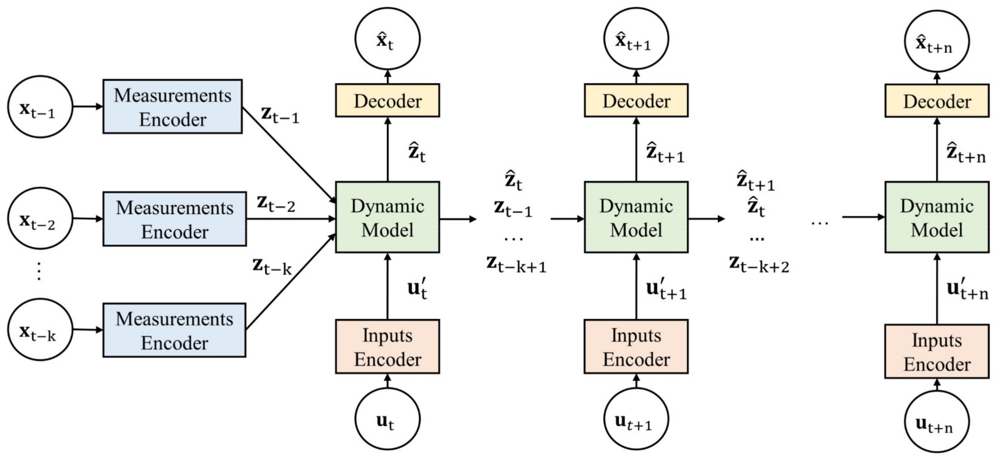
In this section, we discuss the LSDNN model. Figure 1 shows the schematic of the proposed LSDNN architecture, which consists of two parts: an encoder–decoder structure for mapping the original data to latent variables (and vice versa) and a latent-space dynamic model. In the LSDNN model, the encoder–decoder structure captures cross-correlations among measurements and enables a latent-space representation. Let ${\mathit{x}}_t\in {\mathbb{R}}^m$ denote a vector of $m$ measured variables at time $t$, ${\mathit{z}}_t\in {\mathbb{R}}^h$denote a vector of $h$ dimensional latent variables with $h<m$ at time $t$, and ${\mathit{u}}_t\in {\mathbb{R}}^n$ denote a vector of exogenous variables such as control adjustments and ambient temperature at time $t$. In the beginning, the measurement encoder brings the past measured variables into the $h$-dimensional latent space in which the latent dynamics are propagated, and predictions are made. In addition, since the dimensionality of the exogenous variables may be different from $h$, an input encoder is used to map the exogenous variables $\mathit{u}$ to a vector ${\mathit{u}}^{\prime }\in {\mathbb{R}}^h$.

Once the predictions are made through the latent-space dynamic model, the decoder maps them back to the original data space. For each time step, the model uses the same measurement encoder, input encoder, and decoder. In our model, the encoders are represented using dense neural network layers followed by a hyperbolic tangent activation function as follows:

$${\mathit{z}}_t=f^{me}\left({\mathit{x}}_t\right)= \tanh \left({\mathit{W}}^{me}{\mathit{x}}_t+{\mathit{b}}^{me}\right)$$

(1)

$${\mathit{u}}_t{}^{\prime }=f^{ie}\left({\mathit{u}}_t\right)= \tanh \left({\mathit{W}}^{ie}{\mathit{u}}_t+{\mathit{b}}^{ie}\right)$$

(2)

where ${\mathit{W}}^{me}\in {\mathbb{R}}^{h\times m}$, ${\mathit{b}}^{me}\in {\mathbb{R}}^h$, ${\mathit{W}}^{ie}\in {\mathbb{R}}^{h\times n}$, and ${\mathit{b}}^{ie}\in {\mathbb{R}}^h$. The decoder is also a dense layer that decodes the predicted latent state ${\widehat{\mathit{z}}}_t$at time $t$ to the predicted measured variables ${\widehat{\mathit{x}}}_t$ at time $t$. As a result, the decoder can be represented as

$${\widehat{\mathit{x}}}_t={\mathit{W}}^{de}{\widehat{\mathit{z}}}_t+{\mathit{b}}^{de}$$

(3)

where ${\mathit{W}}^{de}\in {\mathbb{R}}^{m\times h}$and ${\mathit{b}}^{de}\in {\mathbb{R}}^m$.

To capture the autocorrelation, describe the evolution of the latent states, and account for the effect of exogenous variables on the latent dynamics, a latent-space dynamic model was used in the LSDNN model. The propagation of latent-space dynamics is represented using a NARX, which has the form

$${\widehat{\mathit{z}}}_t=f\left({\mathit{z}}_{t-1},\dots ,{\mathit{z}}_{t-D_z},{\mathit{u}}_t{}^{\prime },\dots ,{\mathit{u}}_{t-D_u}{}^{\prime } \right)$$

(4)

where ${\widehat{\mathit{z}}}_t$ is the one-step-ahead prediction at time $t$, $D_z$ is the order of the latent state, and $D_u$ is the input order. To perform multi-step-ahead prediction in the latent space given the trajectories of future exogenous variables, a recursive prediction strategy was used [24], where the one-step-ahead prediction from the dynamic model was treated as a true latent state and fed into the dynamic model recursively.

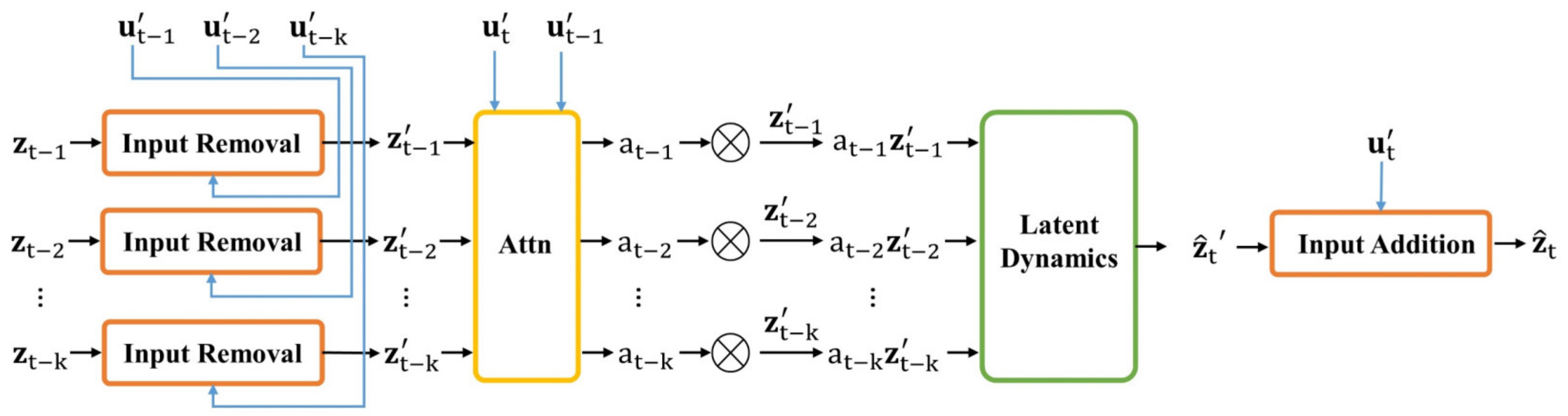
In this study, we considered a NARX network with an input order of $k$ and set the $D_{z }$to be $k$. In the neural network representations of NARX, the nonlinear function $f$ is approximated using a dense layer, where the input layer receives the concatenated vector of past measured variables and exogenous variables. As a result, with this representation, the number of weights of the dense layer is $\left(kh+\left(k+1\right)h\right)h$. If the latent dimension $h$ is large, the large number of weights may lead to overfitting issues and take longer to train the neural network. We decided to alleviate this problem by taking advantage of the characteristics of the time-series data collected from the geothermal power plant. The exogenous variables were highly correlated with the measured variables in the data, which meant that they were also correlated with the series of encoded latent states. To take advantage of this characteristic, we separated the effect of exogenous variables on the latent states and the residual dynamics of the latent states, which made the model more interpretable and less complex. This can be achieved by first forming residual states ${\mathit{z}}^{\prime }\in {\mathbb{R}}^h$by removing ${\mathit{u}}^{\prime }$ from $\mathit{z}$, then concatenating past $k$ residual states as an input to the dense layer. After the dense layer produces a one-step-ahead prediction, the effect of the exogenous variables at the new time step is added back. Following this approach, the dense layer is used to approximate an autoregressive model of ${\mathit{z}}^{\prime }$, representing the evolution of the residual dynamics that is not accounted for by the encoded exogenous variables ${\mathit{u}}^{\prime }$. As a result, the number of weights in the dense layer is reduced to $\left(kh\right)h$. Furthermore, since the effects of exogenous variables are already included in the encoded measured variables, the effect of ${\mathit{u}}^{\prime }$ must be removed from the encoded variables $\mathit{z}$ prior to being fed to the dynamic model. As a result, the model is able to properly separate the effects of the exogenous variables and the residual dynamics.

In a geothermal power plant, there may be multiple power generation units that share the brine produced by the production wells. Shutting down one of the production wells or one power generation unit may cause sudden changes in brine flow that affect other measured variables. In addition, these changes affect the exogenous variables, such as control setpoints, accordingly. As a result, in the time-series data collected from geothermal power plants, sudden significant changes may occur in some measured variables and exogenous variables. For our proposed dynamic model, oscillations in prediction can occur when sudden changes are made due to the autoregressive nature of the dynamic model. Furthermore, when significant changes happen, the next time step prediction may not require all of the past $k$ latent states, which act as the memory associated with the past dynamics. Hence, we designed an attention mechanism to allow the model to make adjustments, forget some of the past stored latent states, and focus on relevant latent states based on the changes in exogenous variables. The attention mechanism has been an essential part of sequence modeling and machine translation, where it has been used to adaptively select a subset of hidden states while decoding the translation [25,26]. The attention mechanism has also been applied for time-series-forecasting tasks. An attention mechanism is used to combine hidden states to model nonseasonal dependency [27]. In [28], an input attention mechanism was designed to extract relevant input features at each timestep based on the previous encoder’s hidden states. In addition, a temporal attention mechanism was used to select relevant encoder hidden states across all time steps. The attention mechanism can be expressed using dot product, similarity functions, or a multilayer perceptron. In this study, we used a dense layer to implement the attention mechanism. At the prediction step $t$, the input to the dense layer is the concatenated vector of ${\mathit{u}}_t{}^{\prime }$ and ${\mathit{u}}_{t-1}{}^{\prime }$, which are the encoded exogenous variables. The output of the dense layer is a $k$ dimensional vector ${\left[a_{t-1}^{\prime },\dots ,a_{t-k}^{\prime }\right]}^{\mathrm{T}}\in {\mathbb{R}}^k$ in which each element corresponds to a residual state vector. A softmax function is then applied to the output to produce a vector of attention scores ${\left[a_{t-1},\dots ,a_{t-k}\right]}^{\mathrm{T}}\in {\mathbb{R}}^k$. Finally, the adjusted residual states are $a_{t-i}{\mathit{z}}_{t-i}^{\prime }\in {\mathbb{R}}^h$ for $i=1, 2, · · · , k$. As a result, the attention mechanism allows the dynamic model to scale the stored past $k$ residual states based on the changes in encoded exogenous variables between two consecutive time steps. When the exogenous variables change suddenly, the model can focus on relevant past residual states for prediction.

Figure 2 shows the details of the latent-space dynamic model. Given the past $k$ encoded measured variables and the encoded exogenous variables, the one-step-ahead prediction can be represented as

$$\left[{\mathit{z}}_{t-1}^{\prime },\dots , {\mathit{z}}_{t-k}^{\prime }\right]=\left[{\mathit{z}}_{t-1},\dots ,{\mathit{z}}_{t-k}\right]-\left[{\mathit{u}}_{t-1}^{\prime },\dots , {\mathit{u}}_{t-k}^{\prime }\right]$$

(5)

$${\left[a_{t-1}^{\prime },\dots ,a_{t-k}^{\prime }\right]}^{\mathrm{T}}=\tanh \left({\mathit{W}}^a\left[{\mathit{u}}_t{}^{\prime };{\mathit{u}}_{t-1}{}^{\prime }\right]+{\mathit{b}}^a\right)$$

(6)

$$a_{t-i}=\frac{\exp \left(a_{t-i}^{\prime }\right)}{{{\displaystyle \sum }}_{j=1}^k\exp \left(a_{t-j}^{\prime }\right)}, i=1, 2, · · · , k$$

(7)

$${\widehat{\mathit{z}}}_t^{\prime }=\tanh \left({\mathit{W}}^d\left[a_{t-1}{\mathit{z}}_{t-1}^{\prime };\dots ;a_{t-k}{\mathit{z}}_{t-k}^{\prime }\right]+{\mathit{b}}^d\right)$$

(8)

$${\widehat{\mathit{z}}}_t={\widehat{\mathit{z}}}_t^{\prime }+{\mathit{u}}_t{}^{\prime }$$

(9)

where ${\mathit{W}}^a\in {\mathbb{R}}^{k\times 2h}$, ${\mathit{b}}^a\in {\mathbb{R}}^k$,${\mathit{W}}^d\in {\mathbb{R}}^{h\times kh}$ and ${\mathit{b}}^d\in {\mathbb{R}}^h$. Once the model generates the one-step-ahead prediction in latent space, the stored past $k$ latent states are updated by removing the last latent state and adding the newly predicted latent state. Further predictions in the latent space can be made by recursively feeding the new prediction back into the model and updating the past latent states.

3. Prediction Results

In this section, we first demonstrate the prediction capability of the proposed LSDNN using real data collected from a geothermal power plant and discuss the design of the LSDNN structure. The field data were collected from a binary cycle geothermal power plant operated by Cyrq Energy Inc. (Salt Lake City, UT, USA). The data consist of five years of hourly time-series measurements. After removing the missing data points and data collected during shutdown periods, around 20,500 data points were used for training and validation, and the remaining 4000 data points were used for testing. There were 19 measurements collected from the primary cycle, secondary cycle, and the turbine of the power generation unit. Among the 19 variables, we selected the brine outlet flow, the setpoint of the turbine inlet guide vane (IGV), and the R134a pump speed to be part of the exogenous variables for incorporating the changes in the operational settings. In addition, we used the ambient temperature as the fourth exogenous variable, since the efficiency of the plant is highly related to the ambient temperature because of the air-cooling system [4,29]. As a result, multi-step-ahead predictions were performed on the remaining 15 measured variables with given future operation settings and weather forecasts.

Before implementing the final LSDNN structure in PyTorch, sensitivity analysis was first performed to determine the structure of the LSDNN model. There were two hyperparameters: the latent space dimension $h$ and the number of past data points used for predictions $D_z$. For each hyperparameter value, 10 models were trained, and the final prediction accuracy was evaluated based on the validation dataset using the average of the root mean squared errors. It can be observed from Figure 3 that, with a small latent space dimension, the model could not capture all the dynamical patterns in the data, which led to underfitting. On the other hand, if the latent states dimension was too large, the number of parameters in the LSDNN model also increased, leading to overfitting. The sensitivity analysis with respect to $D_z$ showed that a small window size could not effectively encode the information from the past data points to initialize the latent state used for prediction, resulting in large prediction errors. In addition, beyond a window size of 12, further increasing the window size did not help in improving the prediction performance. As a result, after performing the sensitivity analysis, the latent space dimension $h$ was selected to be 10 and the order $D_z$ was determined to be 12, which meant that the model used information from the past 12 timesteps to make predictions. In addition, the prediction horizon $N$ was selected to be 12 during training. After normalizing the measured variables and exogenous variables collected during normal operation between 0 and 1, sequences of data with a length of 24 timesteps were generated for training. The measured variables in the first 12 samples were used to initialize the encoded latent states, and 12 samples of the exogenous variables were also included. The last 12 samples corresponded to the future exogenous variables and measured variables. The model used the exogenous variables to make multi-step-ahead predictions, while the measured variables were used to calculate the prediction errors for backpropagation. We used 15,800 sequences for training and 4000 sequences for validation. For the ith data sequence, we defined the objective function as

$$\min J_i=\frac{1}{N}{\displaystyle \sum }_{k=1}^N\parallel {\mathit{x}}_k-{\widehat{\mathit{x}}}_k\parallel {}^2+\frac{\lambda }{N}{\displaystyle \sum }_{k=1}^N\parallel {\mathit{z}}_k-{\widehat{\mathit{z}}}_k\parallel {}^2$$

(10)

where $N$ is the length of the prediction horizon, $\mathit{x}$ is the vector of the measured variables in the future, $\widehat{\mathit{x}}$ is the predicted measured variables, $\mathit{z}$ is the future latent state, which is encoded from the future measured variables by the measurement encoder, $\widehat{\mathit{z}}$ is the predicted latent state from the latent-space dynamic model, and $\lambda$ is a hyperparameter used to adjust the penalty on the second term. The first term in the objective function is the mean-square-error of the $N$-step-ahead prediction. The second term penalizes the derivation of the predicted latent states from the true latent states calculated using the measurements encoder. When only the first term of the objective function is used, $\widehat{\mathit{x}}$ is forced to stay close to $\mathit{x}$, while $\widehat{\mathit{z}}$ may be different from $\mathit{z}$, given $\widehat{\mathit{x}}$ is the output from the decoder with independent weights to be adjusted. As a result, the second term was used to separate the latent variables from the decoder so that the predicted latent states remained in the latent space, and the decoder was only to map the latent variables back to the original data space. During training, the parameters of the neural network were trained together through standard backpropagation using Adam optimizer [30] with a learning rate of 0.001 and batch size of 128. With the loss function defined for each data sequence in Equation (10), the overall objective function with $M$ data sequences is defined as

$$\min J=\frac{1}{M}{\displaystyle \sum }_{k=1}^M{J}_k$$

(11)

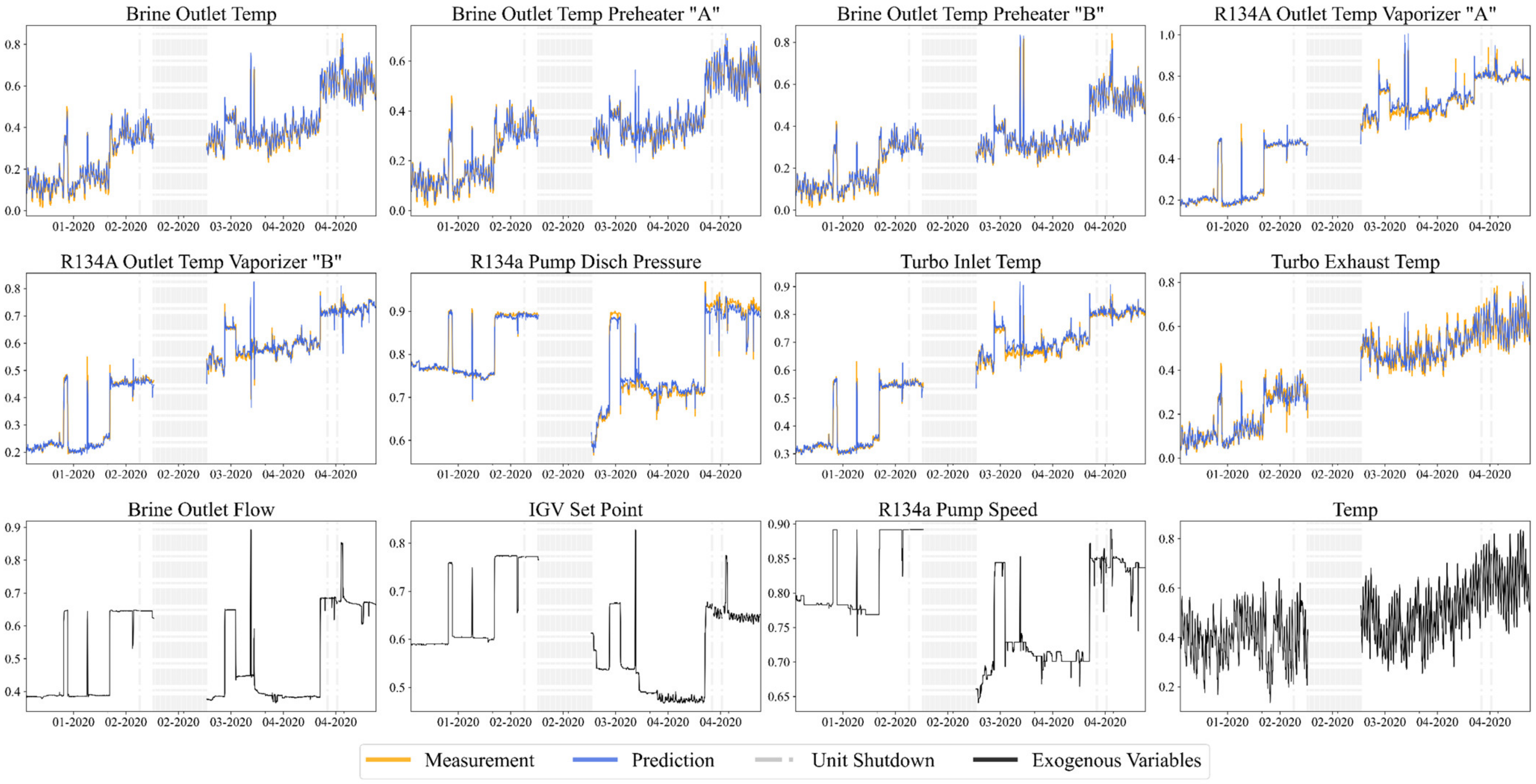
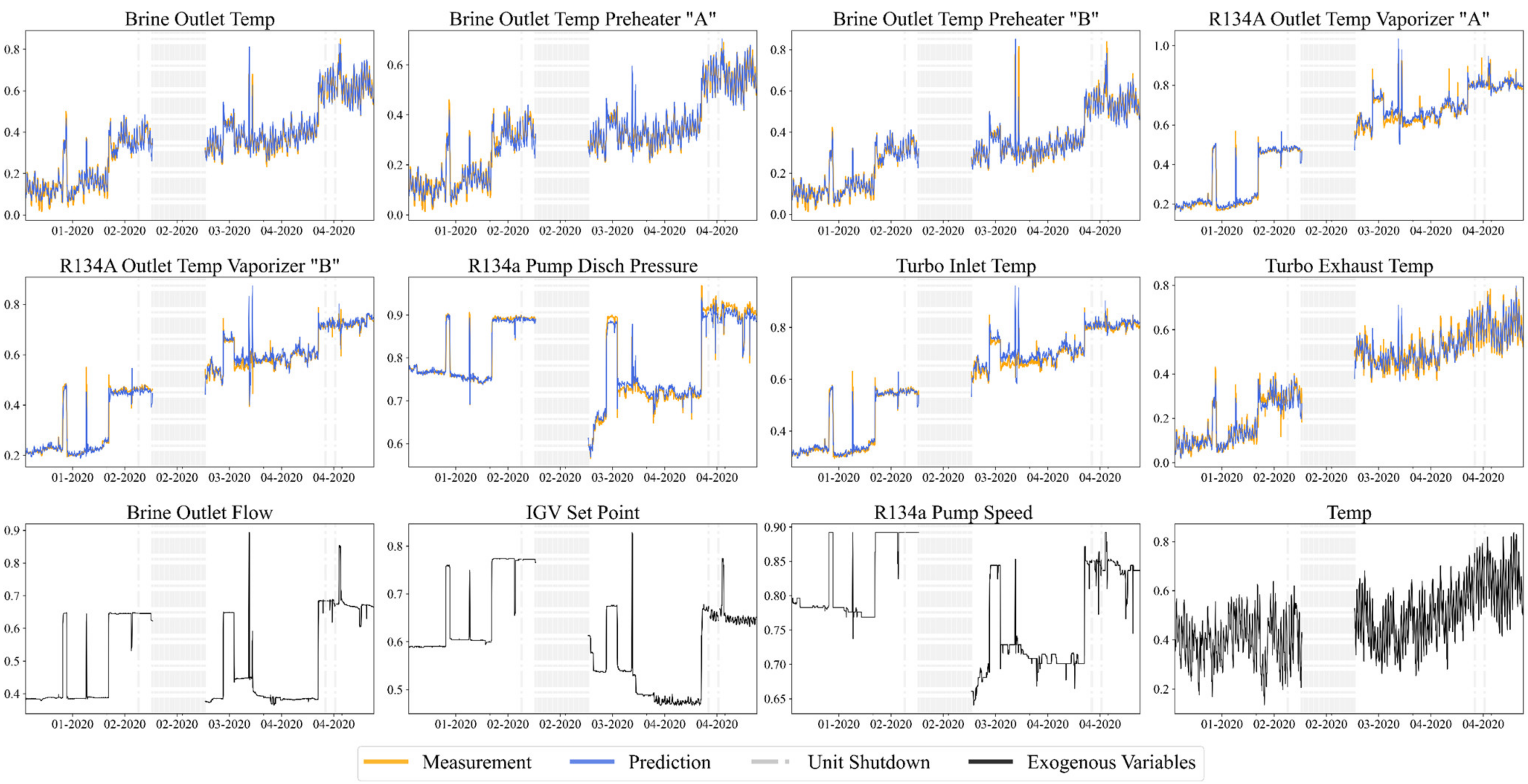
Figure 4 shows the one-step-ahead prediction from the LSDNN on the testing dataset. For better presentation, we plotted the prediction of eight variables among the 15 predicted variables. Similar plots are shown in Figure 5 for 12-step-ahead prediction. The top eight subplots in each figure correspond to eight measured variables, and the bottom four subplots show the exogenous variables. To better display the 12-step-ahead prediction results, Figure 5 was generated in the following way: the model used 12 samples from the past to perform 12-step-ahead prediction. After 12 timesteps, the model received the real measurements from the past and used the most recent 12 samples for forward prediction. As a result, during the 12-step-ahead prediction, the model did not continuously integrate the incoming data at each timestep. It can be observed from the figures that the predictions from the model followed the general trend in the data closely and showed consistent responses to the changes in the operational settings and ambient conditions.

For comparison, we also trained the widely used RNN encoder–decoder model that was proposed in [25], where one LSTM is used to map the input sequence to a vector of fixed dimensionality and another LSTM is used to decode the vector for multi-step-ahead prediction. During training, the inputs to the encoder were the measured and exogenous variables in the past 12 timesteps, and the decoder received the future 12 timesteps of exogenous variables for prediction. The dimension of the hidden vector in the RNN encoder–decoder model was chosen to be 10. To measure the effectiveness of the LSDNN and RNN encoder–decoder for time-series prediction, we considered both the root mean squared error (RMSE) and mean absolute percentage error (MAPE) as evaluation metrics. Let $L$ be the length of the time series. For each measured variable, the RMSE is defined as $\sqrt{\frac{1}{L}{{\displaystyle \sum }}_{i=1}^L{\left(x_i-{\widehat{x}}_i\right)}^2}$ and the MAPE is denoted as $\frac{1}{L}{{\displaystyle \sum }}_{i=1}^L\left|\frac{x_i-{\widehat{x}}_i}{x_i}\right|\times 100\%$. We took the average of the prediction errors of 15 variables to obtain the overall prediction performance for each model. We trained the LSDNN and RNN encoder–decoder 10 times and reported their average performance and standard deviations on the test data. The prediction errors of the 1, 6, 12, and 24-step-ahead predictions are shown in

Table 1. Prediction results of the LSDNN and RNN encoder–decoder.

Prediction Horizon	LSDNN (MAPE)	RNN Encoder–Decoder (MAPE)	LSDNN (RMSE)	RNN Encoder–Decoder (RMSE)
1	$4.1 \pm$0.2%	$4.2 \pm$0.2%	$0.016 \pm$0.001	$0.017 \pm$0.001
6	$4.7 \pm$0.2%	$4.7 \pm$0.1%	$0.019 \pm$0.001	$0.02 \pm$0.001
12	$4.9 \pm$0.2%	$4.9 \pm$0.1%	$0.02 \pm$0.001	$0.02 \pm$0.001
24	$5.3 \pm$0.3%	$5.3 \pm$0.1%	$0.022 \pm$0.001	$0.022 \pm$0.001

. The prediction errors indicate that these two models have similar performances, and both can make accurate multi-step-ahead predictions. In addition, due to the recurrent nature of LSDNN and RNN encoder–decoder models and the similar number of parameters within the models, there was not much difference in the training time. With the selected structures and the same training data, the average time for training both models was around 50 min using one NVIDIA Tesla P100 GPU. However, compared to the RNN encoder–decoder model, the LSDNN model was more interpretable and flexible. It allowed the user to define the dynamics in a low-dimensional latent space and offered the flexibility to use different structures to represent the dynamic model. The use of gate mechanisms in the RNN encoder–decoder model limited the ability to clearly separate the contribution of the exogenous inputs from the hidden states. The design of the LSDNN’s structure lends itself to a more flexible representation of the effect of exogenous variables on the latent states.

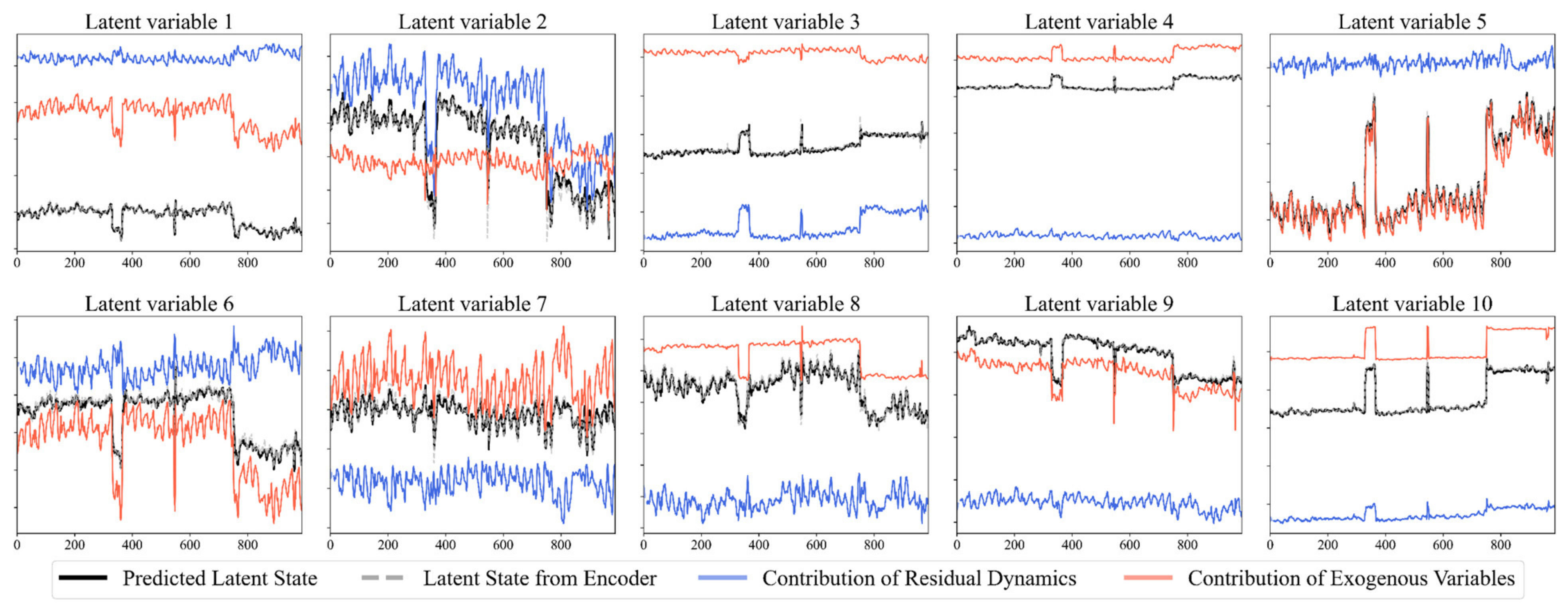
To further interpret the LSDNN model, Figure 6 shows the contribution of residual dynamics and exogenous variables to the latent states when performing one-step-ahead prediction. The blue line represents the contribution related to predicted residual dynamics ${\widehat{\mathit{z}}}_t^{\prime }$ propagated using only the previous states without any effect of exogenous variables. The red line represents the effect of exogenous variables ${\mathit{u}}_t{}^{\prime }$ on the latent states. The final predicted latent state ${\widehat{\mathit{z}}}_t$ was obtained by adding these two values. With a latent variable denoting a sequence of latent states, for latent variables 1, 4, 5, 8, and 9, most of the variations are explained by ${\mathit{u}}_t{}^{\prime }$, whereas, for the rest of the latent variables, both ${\widehat{\mathit{z}}}_t^{\prime }$ and ${\mathit{u}}_t{}^{\prime }$ contribute to the predictions, and the variations are split into the red line and blue line. The grey dotted line is the true latent states that are mapped using the measurement encoder $f^{me}\left({\mathit{x}}_t\right)$. It can be observed that the grey line stayed close to the black line, indicating that, after linearly removing the effects of exogenous variables, making a prediction using the residuals, and adding back the future effects of exogenous variables, the predicted latent states did not deviate from the states encoded from the real measurements.

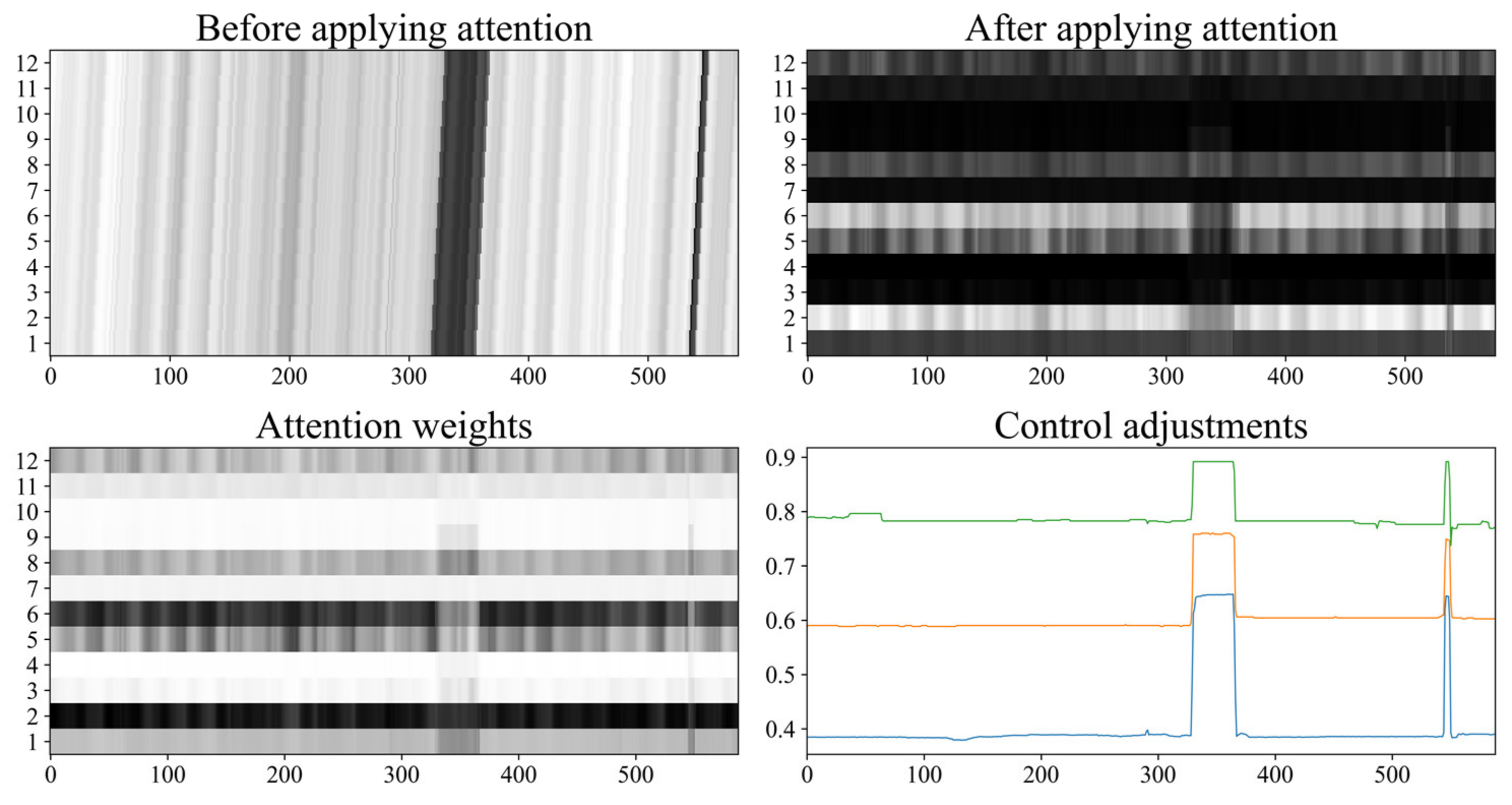
We used one latent variable as an example to visualize the role of the attention mechanism during one-step-ahead prediction, as shown in Figure 7. The top left subplot shows the past 12 latent states $\left[z_{t-1}^{\prime },\dots ,z_{t-12}^{\prime }\right]$ at each timestep before the attention mechanism is applied. Each row in the subplot represents the value of one past latent state. Due to the nature of one-step-ahead prediction, one state value appears 12 times in the plot. For example, if $z_{t-1}^{\prime }$ is the most recent state value at time t, it would show up as the last state value $z_{t-12}^{\prime }$ after 12 timesteps. The subplot on the top right is the updated past 12 latent states $\left[a_{t-1}{z}_{t-1}^{\prime },\dots ,a_{t-12}{z}_{t-12}^{\prime }\right]$ after including the attention mechanism. The subplot on the bottom left shows the attention weights $[a_{t-1},\dots ,a_{t-12}]$ at each timestep. Since the attention weights are related to the changes in the exogenous variables, we also show the control adjustments, which contain sudden significant jumps. It can be observed that the LSDNN model could adjust the attention weights based on the changes and the magnitude of the exogenous variables. For example, for the first 300 time steps in which the controls were not adjusted much, the attention mechanism put more weight on the second and sixth past states. When large changes occurred between timestep 300 and timestep 400, the weights were adjusted accordingly. The same behavior could also be observed when the controls were adjusted at around timestep 550. As a result, the stored past latent states were also scaled based on the attention weights.

4. Fault Detection in a Geothermal Power Plant

To perform fault detection, the general idea is to first build models from data collected during normal operations. Then, control limits are established to define normal operation regions. Finally, the models and the control limits are applied to new data for online fault detection [22,31]. An abnormal event is detected if the output of the models is not within the normal operation regions defined by the control limits. In this paper, the LSDNN model was first trained using data collected from normal operations to extract dynamic variations. As a result, after performing prediction, only normal static variations were present in the prediction errors, where a principal component analysis model could be built to establish the normal control limits on the residuals. When performing monitoring and fault detection on new data, the same LSDNN model, PCA model, and control limits were used.

In this paper, we adopted the well-established PCA-based processing monitoring techniques in [19] to monitor the LSDNN prediction errors. Denoting the one-step-ahead prediction errors of the LSDNN as ${\tilde{\mathit{X}}}^{NN}\in {\mathbb{R}}^{L\times m}$, each row of the error matrix represents a sample at one timestep. Using PCA, the error matrix can be decomposed as

$${\tilde{\mathit{X}}}^{NN}=\mathit{T}{\mathit{P}}^{\mathrm{T}}+{\tilde{\mathit{X}}}^{PCA}=\mathit{T}{\mathit{P}}^T+\tilde{\mathit{T}}{\tilde{\mathit{P}}}^{\mathrm{T}}$$

(12)

where $\mathit{T}$ is the score matrix and $\mathit{P}$ is the loading matrix corresponding to the first $l$ leading principal components (PC). As a result, $span\left\{P\right\}$ is the principal component subspace (PCS) and $span\left\{\tilde{P}\right\}$ is the PCA residual subspace (RS). To monitor the variability in the PCS, Hotelling’s $T^2$ index can be used. It measures the distance to the origin in the principal component subspace, which contains normal variations. For each ${\tilde{\mathit{x}}}^{NN}\in {\mathbb{R}}^m$, the index is defined as

$$T^2={\tilde{\mathit{x}}}^{NN}{}^{\mathrm{T}}\mathit{P}{\mathit{\Lambda }}^{-1}{\mathit{P}}^{\mathrm{T}}{\tilde{\mathit{x}}}^{NN}$$

(13)

$$\mathit{\Lambda }=\mathrm{diag}\left\{{\lambda }_1,\dots ,{\lambda }_l\right\}$$

(14)

$${\lambda }_i=\frac{1}{L-1}{\mathit{t}}_i^{\mathrm{T}}{\mathit{t}}_i$$

(15)

where ${\mathit{t}}_i\in {\mathbb{R}}^L$ is the i^th score vector. For a given significance level $\alpha$, the sample is considered normal if $T^2$is smaller than the corresponding control limit $T_{\alpha }^2$, where $T_{\alpha }^2={\chi }_{l;\alpha }^2$ if $L$ is large [19]. To monitor the variability in RS, the squared prediction error (SPE) index can be used [19]:

$$SPE\equiv \parallel {\tilde{\mathit{x}}}^{PCA}\parallel {}^2= \parallel \left(\mathit{I}-\mathit{P}{\mathit{P}}^T\right){\tilde{\mathit{x}}}^{NN}\parallel {}^2$$

(16)

The SPE index measures variability that breaks the normal process correlation. The sample is considered normal if $SPE\le {\delta }_{\alpha }^2=g{\chi }_{h;\alpha }^2$, where ${\delta }_{\alpha }^2$ is the control limit for the SPE index and

$$g=\frac{{{\displaystyle \sum }}_{i=l+1}^m{\lambda }_i^2}{{{\displaystyle \sum }}_{i=l+1}^m{\lambda }_i}, h=\frac{{({{\displaystyle \sum }}_{i=l+1}^m{\lambda }_i)}^2}{{{\displaystyle \sum }}_{i=l+1}^m{\lambda }_i^2}$$

(17)

In addition, a combined index $\phi$ can be used as a global index that combines the SPE and $T^2$ indices [32]:

$$\phi =T^2\left({\tilde{\mathit{x}}}^{NN}\right)+g^{-1}SPE\left({\tilde{\mathit{x}}}^{NN}\right)$$

(18)

The sample is normal if $\phi \le {\chi }_{h+l;\alpha }^2$.

We applied the fault detection approach to the field data in which two faults occurred in the geothermal power plant. One of them was a fault that occurred in one of the power generation units, and the other was a pump failure at one of the production wells. We trained two LSDNN models for the power generation unit and the production pump using data collected during normal operations. The LSDNN models were used to extract the dynamics and the effects from exogenous variables from available data. Then, the one-step-ahead prediction errors of the fault-free data were calculated. The prediction errors were scaled to have zero mean and unit variance to apply PCA for monitoring the static variations. We selected the number of leading PCs $l$ so that the first $l$ PCs captured 90% of the variances. The SPE, $T^2$, combined index, and their corresponding control limits were then calculated. To monitor test data that contained faults, the trained LSDNN models were applied to the test data and obtain the prediction errors of the test data. With the loadings $\mathit{P}$ and $\mathit{\Lambda }$ from the PCA model built from the normal data, the monitoring indices of the test data were calculated using Equations (13), (16), and (18). Finally, the indices were compared with the control limits to detect the faults.

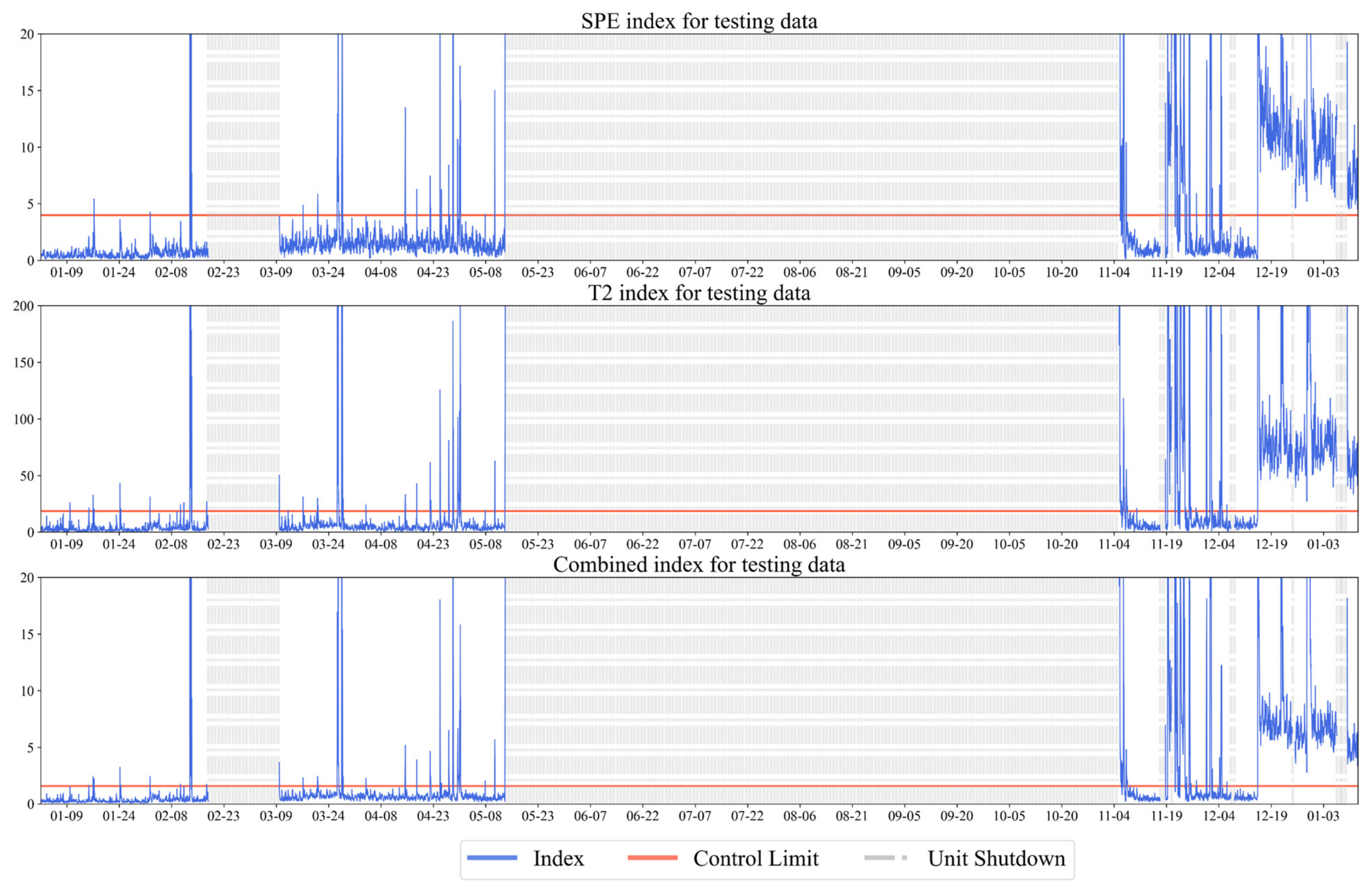
Figure 8 shows the monitoring results for the test data from the power generation unit. The gaps between indices were due to the removal of data during the shutdown periods. At the end of the plot, the power plant operator discovered the fault and stopped the unit for repair. It can be observed that, before 11–19, most of the monitoring indices were below the control limits for all three indices, indicating that the unit was operating normally and there were no abnormal dynamics. A few samples had monitoring indices above the control limits then dropped below the control limits quickly when there were sudden adjustments in the control settings, or the unit was restarted. Since the adjustments were made by the operators, they could easily distinguish these false alarms from the detection of the real faults. In addition, when real faults occurred, the monitoring indices showed strong and consistent signatures, which were different from the false detections. The fault document that was provided by the operator showed that the unit was underperforming around 11–19, which could also be observed in the monitoring indices. Around 12–15, all three monitoring indices rose above the control limits and stayed above the limits until the plant was shut down for repair, which meant that a fault occurred around 12–15 and persisted until the operators discovered the fault.

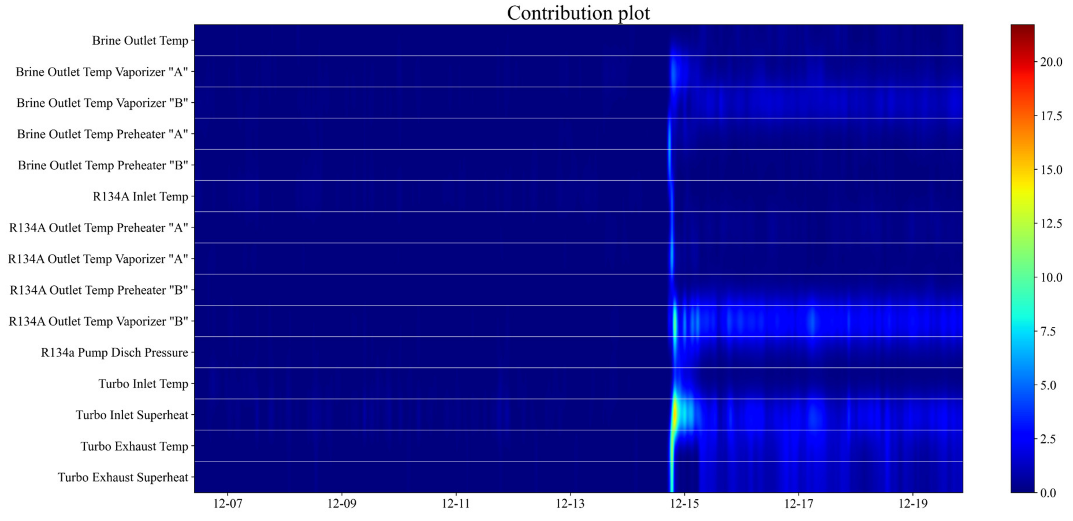
After a fault is detected, the next step is to identify the location of the fault. Contribution plots are well-known tools for fault identification [20,33,34]. From the definition of SPE,

$$SPE\left({\tilde{\mathit{x}}}^{PCA}\right)={{\displaystyle \sum }}_{i=1}^m{({\tilde{x}}_i^{PCA})}^2={{\displaystyle \sum }}_{i=1}^{m}SP{E}_i$$

(19)

where $SP{E}_i$ is the contribution of the $i$th variable in the contribution plot for SPE. For better visualization, we plotted a 2D contribution plot that collected each variable’s contribution for multiple timesteps, shown in Figure 9. On around 12–15, the variable turbo inlet superheat showed the greatest contribution to the SPE. After 12–15, the variables turbo inlet superheat, R134A outlet temperature of vaporizer B, and brine outlet temperature at vaporizer B had the largest contributions, indicating that they were either the major contributors to the fault or affected by the fault.

We followed the same fault detection procedure for monitoring a production well pump. From the fault document, maintenance was performed on the pump from 03–20 to 03-27, and pump failure occurred on 09–26. Figure 10 shows the one-step-ahead prediction results of the measured variables of the pump. Before maintenance, the trained LSDNN model provided accurate predictions. However, offsets in the predictions could be observed in some of the variables after maintenance, indicating changes in the pump’s performance. While the pump components and the nature of the repair are unknown, maintenance, such as sensor recalibration and replacing new components, can cause offsets in the prediction results. However, the underlying physical relationships between different measured and exogenous variables are expected to remain the same before and after maintenance. It can be observed in the prediction results that, even though the offsets existed, the predictions followed similar trends to the measured variables, indicating that the LSDNN model learned the underlying dynamics. Since the dynamics remained the same and the fault monitoring relied on the dynamic relationships and static correlations, we performed the same fault monitoring procedure to determine if the proposed procedure could detect a fault without retraining the LSDNN model. Figure 11 shows the three monitoring indices. It can be observed that the $T^2$ and the combined index rose above their corresponding control limits immediately after maintenance was performed. However, the SPE index gradually grew above the control limit between 08–06 and 08–21. Since the $T^2$ index was used to monitor the leading PCs, it measured the distance of the sample to the origin in the PCS. If a sample exceeded the $T^2$ control limit, it meant that the sample shifted away from the origin in the PCS, but the correlation structure was not violated. On the other hand, the SPE was used to monitor the RS and measure the variability that breaks the correlation relationships. As a result, if the $T^2$ index of a sample is above the $T^2$ control limit but the SPE index lies below the SPE control limit, it could indicate a fault or shift in the operating region [19]. In this pump-related application, we know that maintenance caused the offsets in the prediction errors, which then caused the shift in the PCs. As a result, the $T^2$ index exceeding the control limit did not indicate a fault. Since the combined index was also related to the $T^2$ index, we should only use the SPE for fault detection in this case. Hence, the SPE index exceeding the control limit between 08–06 and 08–21 indicated a fault occurred which broke the correlation structure.

Both the fault detection results for the power generation unit and production pump showed that the proposed fault detection procedure could detect abnormal dynamics before the faults were discovered in the field by the operators. As a result, if the fault detection procedure can be implemented in a geothermal power plant, it is able to detect faults earlier, possibly preventing unscheduled shutdowns or catastrophic failures of equipment.

5. Conclusions

In this paper, a latent space dynamic neural network model was proposed for multi-step-ahead prediction. The model structure was designed based on the characteristics of time-series data collected from geothermal power plants. An encoder–decoder structure was implemented to map the original data to a reduced-dimension latent space in which the dynamics of the power generation process were represented. The predictions were made in the latent space using a dynamic model. In the dynamic model, the effects of the exogenous variables were linearly separated from the latent states to reduce the model complexity and improve interpretability. We also used an attention mechanism to adaptively change the stored latent states based on changes in exogenous variables, which gave the model more flexibility when predicting sudden changes in the measured variables. The prediction performance of the LSDNN on a geothermal power plant dataset was compared with a popular RNN encoder–decoder structure with LSTM. We also proposed a fault monitoring procedure based on the one-step-ahead prediction results of the LSDNN model. First, the LSDNN model was used to extract the dynamics and remove autocorrelations from the time-series data. Then, PCA-based fault detection techniques were applied to the residuals to monitor the static variations. The fault detection procedure was applied to two known faults corresponding to a power generation unit and a production pump. The results show that, in both cases, signatures of abnormal dynamics can be detected before the faults are discovered in the field.

The proposed LSDNN model can be extended to include other structures for the dynamic model in the latent space. Additional studies are needed to explore fault prediction and the possibility of an advance fault warning system based on multi-step-ahead prediction. In addition to fault prediction and detection, the model can be extended to include fault diagnosis to inform possible causes of a potential failure or abnormal events. Another topic that was not explored in this paper was retraining and updating the model with incoming data, which is expected to improve the predictive power of the model. Furthermore, in the case study of the production pump failure, the predictions were affected by maintenance, and retraining could be used to adapt the dynamics to the changes due to maintenance. Finally, the LSDNN model could also be used as a data-driven predictive model in broader applications, such as model predictive control and optimization of the geothermal power plants.