Article

Risk Contagion between Global Commodities from the Perspective of Volatility Spillover

1
School of Business, Yangzhou University, Yangzhou 225127, China
2
WA Franke College of Business, Northern Arizona University, Flagstaff, AZ 86011, USA
*
Author to whom correspondence should be addressed.
Energies 2022, 15(7), 2492; https://doi.org/10.3390/en15072492
Submission received: 14 February 2022 / Revised: 12 March 2022 / Accepted: 25 March 2022 / Published: 28 March 2022
(This article belongs to the Special Issue Behavioral Models for Energy with Applications)

Abstract

:
Prices of oil and other commodities have fluctuated wildly since the outbreak of the COVID-19 pandemic. It is crucial to explore the causes of price fluctuations and understand the source and path of risk contagion to better mitigate systemic risk and maintain economic stability. The paper adopts the method of network topology to examine the path of risk contagion between China’s and foreign commodities, focusing on the dynamic evolution and transmission mechanism of risk contagion during the pandemic. This research found that among China’s commodities, energy, grain, and textiles are net recipients of risk contagion, while chemical products and metals are net risk exporters. Among international commodities, industries have positive risk spillover effects on metals and textiles. During the first phase of the pandemic, China’s commodities were the main exporters of risk contagion. However, international industries and metals became the main risk exporters and exerted risk spillover on China’s commodities in the second phase of the pandemic. Moreover, based on total volatility spillover index of commodities, the risk contagion among the commodities follows three paths: “interest rate → commodities → money supply”, “China’s economic expectation → commodities → foreign economic expectation”, and “commodities → consumer confidence”.

1. Introduction

In recent years, global public emergencies and extreme events have erupted frequently, causing serious impacts on the social stability of countries worldwide and global economic development. The resultant disturbances were often rapidly transmitted to financial markets, causing strong turbulence in financial markets [1,2]. The novel coronavirus pneumonia in 2020, also called COVID-19, ravaged the world, plunging the global economy into the worst recession since World War II and causing dramatic fluctuations in global commodity markets, which triggered a sharply increased systemic risk within commodity markets. Since the beginning of 2020, the overall fluctuation of commodity prices has exhibited a large “V” shape, with sharp rises and falls. On 21 April 2020, the US WTI crude oil futures contract fell to the first negative settlement price in history: −$37.63. On the other hand, commodity prices bottomed and rebounded, showing an accelerated growth trend. From 1 May 2020 to 5 May 2021, the Commodity Research Bureau (CRB) Composite Index rose by 51.84% from 354.23 to 537.88. The prices of crude oil, iron ore, copper, and some agricultural products repeatedly hit record highs, causing a great impact on the productions and operations of enterprises of downstream companies [3]. Since May 2021, the State Council of China has highlighted rising commodity prices three consecutive times, calling for strengthening market regulation and ensuring stabilization of the supply and prices.
The COVID-19 pandemic is the immediate cause of the abnormal fluctuation of commodity prices. Although most countries took extensive measures to prevent the spread of the pandemic, it still exerted a continuous impact on the global economy. With the sharp increase in systemic risk in commodity markets, it is urgently crucial to study the risk contagion path of the market to effectively monitor the sources of risk contagion and explore the underlying causes of price fluctuation to better help international investors and policymakers carry out risk management, asset allocation, and policy adjustment in time.

2. Literature Review

The key to the study of financial risk contagion is the effective measure of risk spillover. The GARCH model proposed by Bollerslev in 1986 has been widely used to measure the volatility spillover effect; however, this approach does not consider the distribution of return under extreme risks. Since the G30 group put forward the VaR (value at risk) method to measure market risks in 1993, the VaR method has been widely used in risk measurement. The expected shortfall (ES) proposed by Acerbi and Tasche (2002, [4]) has been used to further measure the average loss of a portfolio in extreme cases based on VaR to offer a more complete characterization of the risk of extreme loss of a portfolio. Hong et al. (2004, [5]) studied the risk spillover effect between China’s stock market and other stock markets in the world through the stock market closing index, and Zhang et al. (2010, [6]) used the VaR method to measure the risk of the agricultural product market in China. However, the VaR method may underestimate the risk during the financial crisis, and it cannot accurately measure the risk spillover between financial institutions. Adrian and Brunnermeier (2008, [7]) constructed the CoVaR model of conditional risk value to attempt to measure the risk faced by the whole financial system during the crisis of certain financial markets that provided a new idea for risk measurement. Based on this method, Gao and Pan (2011, [8]) measured the contribution of 14 listed companies to systemic risk. Mao and Luo (2011, [9]) conducted an empirical study on the risk spillover between China’s banking and the securities industries and found that there was a strong two-way risk spillover.
Although CoVaR solves the challenge of measuring risk overflow from the financial system under extreme risks, it was only applicable for measuring the risk spillover between two markets but was inappropriate for measuring risk contagion among multiple markets. Li et al. (2020, [10]) explored the systematic risk and risk contagion effect of Chinese banks and enterprises through the debt rating method. Baruník and Křehlík (2018, [11]) used the time–frequency connectedness approach to measure the frequency dynamics of financial connectedness and systemic risk. Additionally, a novel quantile spillover approach was introduced to measure the tail risk connectedness [12]. Diebold and Yilmaz [11,12,13,14,15] proposed and improved the method of constructing spillover index through generalized prediction error variance decomposition that investigated the correlation of financial risks from the perspective of network topology. It has been applied to study the risk spillover between different financial markets, financial institutions, and economies [16,17,18,19]. This method can measure the direction, scale, and intensity of risk spillover and eliminate the effect of variable order on the orthogonal decomposition results, overcoming the shortcomings of the lack of power and direction in most complex networks and making the network more realistic [20].
The COVID-19 pandemic inspired a new stream of literature focusing on the impact of the global public emergency on financial markets. The pandemic has had a huge impact on the global macroeconomic environment [21], and its impact on the financial operation is mainly reflected in the three stages of expected shocks, entity conduction, and policy digestion [22]. At the same time, common risk exposure and asset allocation adjustment have further impacted the financial system [23]. In terms of risk contagion, Yang et al. (2020, [24]) adopted dynamic risk spillover methods to explore the dynamic risk transmission among various sectors of China’s financial market and major global financial markets during the COVID-19 pandemic. Fang and Jia (2021, [25]) analyzed the risk changes in the global and Chinese foreign exchange markets under the influence of the COVID-19 pandemic using the LASSO method and explored the amplification or mitigation effects of financial markets, the real economy, and policies on this impact.
A body of literature on the impact of the pandemic on the commodities market has also emerged. Kamdem et al. (2020, [26]) found that the number of confirmed cases and deaths caused by the pandemic had a great impact on the volatility of commodity prices. Dmytrów et al. (2021, [27]) used the dynamic time warping (DTW) method to assess the similarity between the time series of energy commodity prices and daily COVID-19 cases. Some studies confirmed that uncertainty related to a pandemic had a strong negative impact on the volatility of commodity markets, especially on crude oil, energy products, etc. [28,29], while the effect on gold and greenhouse gas emissions were not significant [28,30]. Liu et al. (2021, [31]) used the time-varying connectedness measurement to investigate the spillover effects among three commodity assets (oil, gold, and corn) and three financial assets in China and the US during the pandemic. Umar et al. (2021, [32]) constructed a coronavirus panic index and analyzed the interdependencies between the index and the movements of the prices of five traditional categories of commodities (energy, agriculture, livestock, precious metals, and nonprecious metals) to study how the COVID-19 pandemic influenced the volatility of commodities. Borgards et al. (2021, [33]) detected the overreaction behavior of 20 commodity futures in two separate periods (pre-COVID-19 pandemic and during COVID-19 pandemic).
As can be seen above, the commodity markets have become a new research focus since the outbreak of the COVID-19 pandemic. The recent research is mostly focused on the dynamic connectedness between the pandemic and the price fluctuation of the commodity markets, and the markets involved are mainly metal, energy, agricultural futures [26,27,28,29,30,31,32,33]. Although some studies have investigated the risk spillovers within the commodity markets, the impact of the pandemic has not been systematically and comprehensively studied, especially the discussion on the risk contagion mechanism within the commodity markets and the risk transmission pathways.
Hence, our research adopts the network topology analysis method and constructs the volatility spillover matrix to investigate the dynamic evolution of risk contagion in the commodities market. We focus on China and international commodity markets to compare the differences and similarities of volatility spillover within the two markets and explore the volatility spillover relationship between them. We also divide the full sample into different subsamples according to the important time points of the COVID-19 pandemic to explore its impact on the commodity markets during these phases. Moreover, our paper discusses the mechanism of risk contagion in the commodity markets through nonlinear causality analysis and reveals the risk transmission pathways, which is another important novel contribution and complement to the existing studies. It also provides evidence on the internal relationship between commodity markets and monetary policy as well as economic expectation. The remainder of the paper is organized as follows: Section 3 formalizes the research method and data description. Section 4 discusses the empirical analysis focusing on the dynamic evolution and paths of risk contagion in the commodities market, and Section 5 contains the conclusions.

3. Research Method and Data Description

3.1. Construction of Risk Spillover Index

In this paper, the volatility spillover index proposed by Diebold and Yilmaz (2009, [13]) is used to measure the risk spillover effect between different variables by variance decomposition. Following similar notations used in Diebold and Yilmaz (2014, [15]), the covariance stationary VAR (p) model of the N-dimensional variable Xt expressed in moving average form as shown below is considered:
X t = i = 0 A i ε t i
where A0 is an N × N unit matrix, Ai is the N × N moving average coefficient matrix for i > 0 while Ai = 0 for i < 0, and εt is an N-dimensional independent and identically distributed white noise error with a time-invariant positive definite variance matrix. The KPPS [34,35] H-step-ahead forecast error variance, θ i j H , of the variable Xt due to shock to the variable Xj is measured by
θ i j H = σ j j 1 h = 0 H 1 ( e i A h Σ e j ) 2 h = 0 H 1 ( e i A h Σ A h e i )
where i, j = 1, …, N, ∑ is the variance matrix of the error vector ε, σjj is the standard deviation of the error term of the j-th equation, and ei is the N × 1 dimension unit vector. Since the elements in each row of the variance decomposition do not add to one, Diebold and Yilmaz (2014, [15]) normalize each entry by the row sum as:
θ ˜ i j H = θ i j H / j = 1 N θ i j H
such that j = 1 N θ ˜ i j H = 1 ,   i , j = 1 N θ ˜ i j H = N .
Using the volatility contribution of the KPPS variance decomposition above, the total volatility spillover index is constructed as:
S H = i , j = 1 i j N θ ˜ i j H i , j = 1 N θ ˜ i j H 100 = i , j = 1 i j N θ ˜ i j H N 100
to measure the total bidirectional impact contributions of the mutual spillover effects between all asset classes to the total volatility.
Next, the total unidirectional contributions to volatility spillovers from different assets is measured using the unidirectional volatility spillover indexes received by market i from all other markets j (j ≠ i) as:
S i   H = j = 1 j i N θ ˜ i j H i , j = 1 N θ ˜ i j H 100 = j = 1 j i N θ ˜ i j H N 100
In a similar way, the total unidirectional volatility spillover index transmitted by the market i to all other markets j (j ≠ i) is measured by
S   i H = j = 1 j i N θ ˜ j i H i , j = 1 N θ ˜ j i H 100 = j = 1 j i N θ ˜ j i H N 100
These total unidirectional volatility spillover indexes are seen as decompositions of the total spillover into either to or from a specific source.
Further, the total net volatility spillover of market i to all other markets j (j ≠ i) is measured by the total net volatility spillover index:
N S i H = S i H S i H
This total net volatility spillover measures the difference between the total volatility shocks delivered to all other markets and the shocks received from all other markets. Therefore, the net pairwise directional volatility spillover index from market j to market i can be calculated as:
N S j i H = ( θ ˜ j i H i , k = 1 N θ ˜ k i H θ ˜ i j H i , k = 1 N θ ˜ i k H ) 100 = ( θ ˜ j i H θ ˜ i j H N ) 100
which is the difference between the gross volatility shocks transmitted from market i to market j and those transmitted from market j to market i. This is used to measure the net volatility spillover contribution of market i to market j.
Based on this, the total net volatility spillover that market i transfers to all other markets j for j ≠ i, T N S O U T , i H , and the total net volatility spillover that market i receives from all other markets j for j ≠ i, T N S I N , i H , can be computed as:
T N S O U T , i H = N S i H = j = 1 j i N N S j i H
T N S I N , i H = N S i H = j = 1 j i N N S i j H

3.2. Data Description

To examine the risk contagion between China’s and foreign commodities and explore the dynamic evolution of risk contagion under the public emergency of the COVID-19 pandemic, the main commodities, which include energy, metals, grain, textiles, and chemical products, traded on China’s commodity futures market are selected as the representatives for China’s commodity markets. On the other hand, the daily logarithmic returns of the indexes compiled by the Commodity Research Bureau (CRB) serve as the representative indexes of global commodity markets [36]. Four indexes are selected: textiles, metals, food, and industrial. In this paper, CFCI and CRB are used to distinguish between China’s and foreign commodity indexes. We collected 3606 daily data points from 14 November 2005 to 19 March 2021, from the Wind database. We also use the dynamic value at risk (VaR) of daily logarithmic return to test the robustness of the model used in this paper. The forecast period reported in this paper is 10 days. The results remain stable and qualitatively the same after changing the number of forecast periods.
The descriptive statistics of the logarithmic returns in the sample are shown in Table 1. The table shows that the sample average yield of all varieties of commodities is near 0 and positive except CFCI Textiles and CFCI Chemical Products. The standard deviation of the Chinese varieties is significantly greater than that of the international varieties, indicating that the yield of Chinese varieties has much higher volatility. All varieties have leptokurtic distributions with fatter tails than a normal distribution. Most notably, the degree of skewness of CFCI Grain is much greater than that of other varieties and has the largest kurtosis coefficient, indicating that the yield of CFCI Grain has a thick-tail distribution that is skewed to the right with outliers in the upper tail. In general, the logarithmic return of each variety passes the augmented Dickey–Fuller test for unit root, indicating that the method used in this paper is appropriate. The Jarque–Bera test for normality also rejects the null hypothesis of a normal distribution, confirming that the distributions of all commodities deviate from the normal distribution.

4. Empirical Analysis

4.1. Static Analysis of Volatility Spillover

Using the volatility spillover indexes defined in Equations (1)–(10), we calculated the spillover effects of the nine categories of commodities and conducted the spillover effect analysis. The results are listed in Table 2.
From the perspective of the “OUT” spillovers, the total outward volatility spillover of CRB Industrials to all other commodities is the largest with an index value of 75.6, followed by CFCI Chemical Products and CFCI Metals, at 65.34 and 59.93, respectively. The total outward volatility spillover of CFCI Grain and CRB Food is small, at only 15.71 and 17.88, respectively. It can be seen from the unidirectional volatility spillover between any two varieties that the internal spillovers of commodities within China’s commodities or foreign commodities are almost always significantly greater than the volatility spillovers between China’s and foreign commodities. Focusing on the internal impact, China’s commodities are almost most affected by the volatility spillovers from CFCI Chemical Products, followed by CFCI Metals; foreign commodities are most affected by CRB Industrials.
From the perspective of “IN” spillovers, CRB Industrials, CFCI Chemical Products, and CFCI Metals are most affected by all other commodities, at 58, 56.99, and 56.44, respectively. CFCI Grain and CRB Food are least affected by all other commodities, at 23.79 and 20.63, respectively.
The ratio of the total volatility spillover of all commodities to others excluding themselves to the total volatility spillover including themselves shows that 43.7% of the forecast error variance comes from the spillover effect between the commodities.
Based on Table 2, we further compute the net pairwise spillover index between any two varieties using Equation (8) and the total net volatility spillover using Equations (9) and (10), and the results are presented in Table 3.
Notice that the values of TNSIN are the exact opposite of TNSOUT in Table 3. From Table 3, we can see that during the period 2006 to 2020, the total net outward volatility spillover of CRB Industrials is the largest with an TNSIN index value of 17.6, followed by CFCI Chemical Products at 8.36. CFCI Textiles, Grain, and Energy are net recipients of volatility risk with TNSIN at 7.38, 8.08, and 8.6, respectively. From the perspective of the mutual spillover relationship among Chinese commodities, the net spillover indexes of CFCI Metals and CFCI Chemical Products to other commodities are positive, occupying the role of the risk exporter in the risk contagion among China’s commodities. CRB Industrials is the main exporter of risk from the perspective of the mutual spillover relationship among foreign commodities. From the perspective of the spillover relationship between China’s and international commodities, the net risk spillovers of foreign commodities on Chinese commodities are generally positive, indicating that China’s commodity market is a recipient of international risk from foreign markets in general.

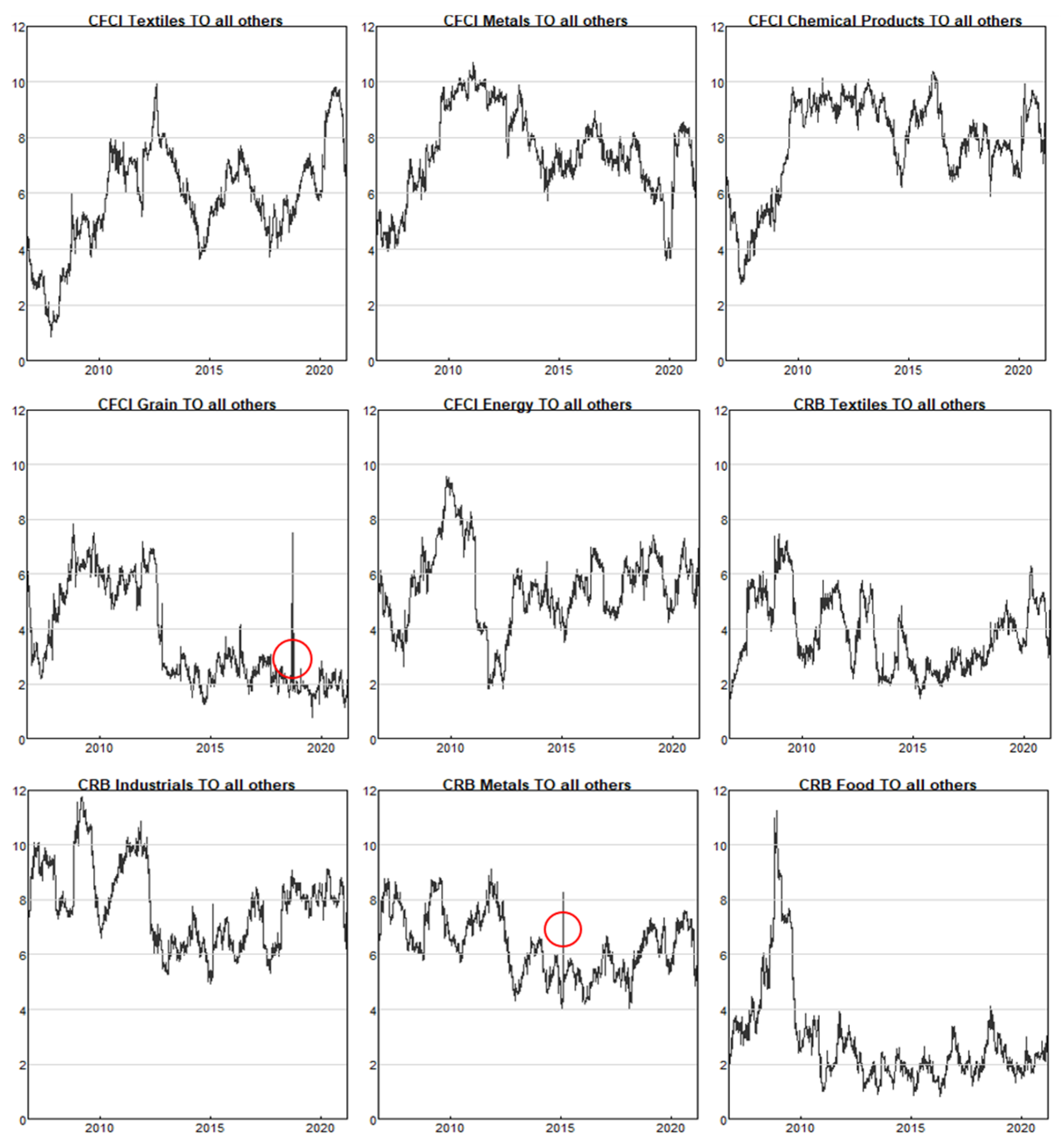
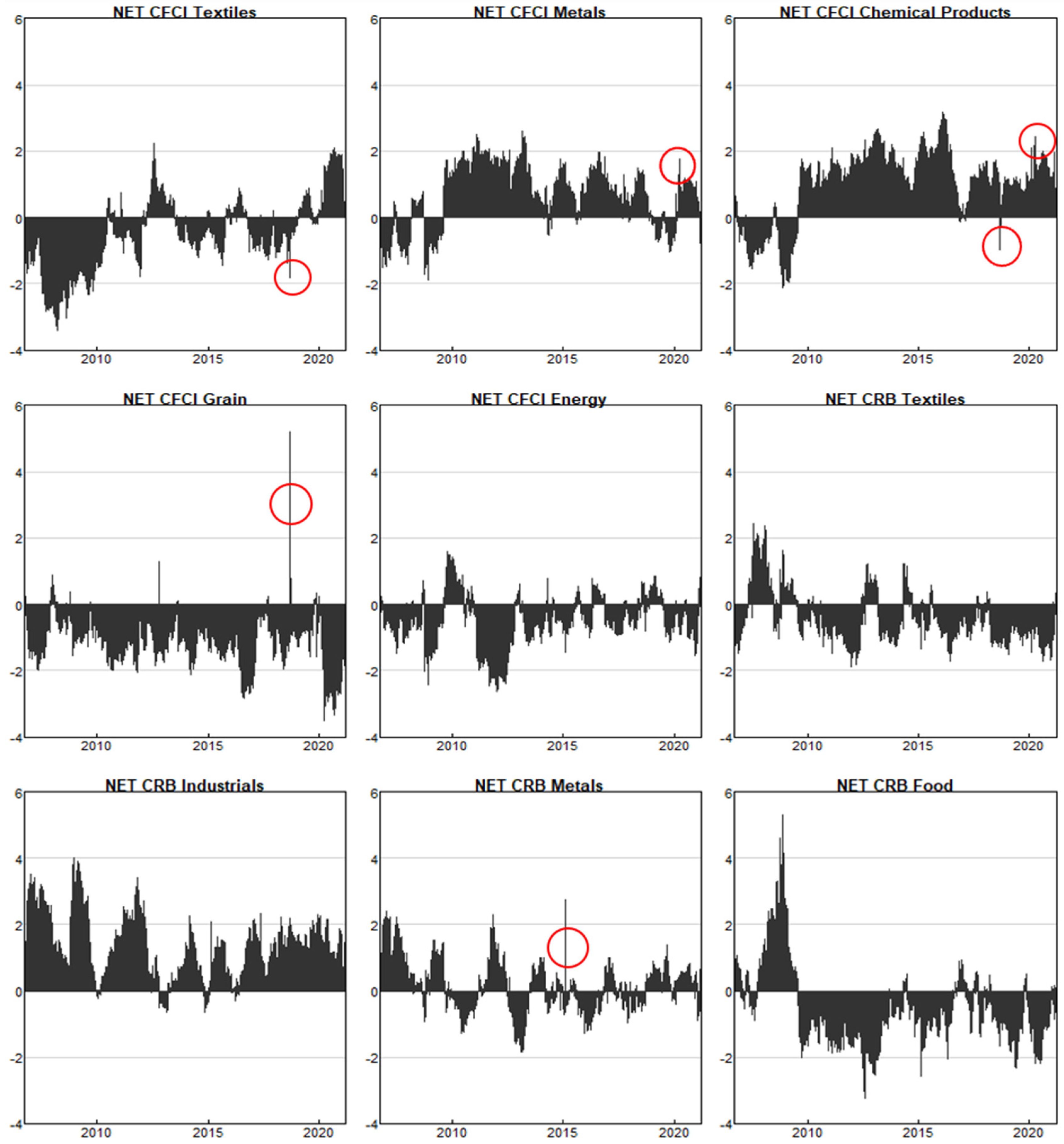
4.2. Dynamic Analysis of Volatility Spillover

We adopt the practice of a rolling window to calculate the dynamic change of the total volatility spillover index in the selected sample interval and analyze the time trend of the risk spillover. The results are shown in Figure 1. The horizontal axis date is the end date of the rolling window.
Figure 1 shows that the total spillover index calculated based on the logarithmic rate of return fluctuates in the range 38 to 70, while that calculated based on VaR fluctuates slightly more with a range between 35 and 80, but the overall trends are basically the same. It can be seen that major public events have varying degrees of impact on the risk spillover of the commodities market. In 2008, the financial crisis swept the world and had a huge impact on the commodities market. Among the major varieties, energy, chemical products, and metals were the most severely impacted and shrank sharply, resulting in a sharp increase in the total volatility spillover index in the second half of 2008 that persisted at a high level until 2013. Similarly, the Japanese earthquake in March 2011, the major flash crash of the stock markets in 2015, and Brexit in June 2016 also had an impact on the commodities market, albeit the impact was relatively short-term.
At the beginning of 2020, impacted by the COVID-19 pandemic, China’s commodity prices fell sharply, and many varieties broke their daily limit. With the spread of the pandemic, the world economy suffered a heavy blow, and international commodity markets experienced huge fluctuations. Since the start of the COVID-19 pandemic, the total volatility spillover index of the commodities market has increased significantly, with an average total spillover index of about 60, which is second only to the financial crisis in 2008. The impact of the COVID-19 pandemic on the commodities market is significant and lasting, and the systemic risk in the commodities market has increased significantly.
Next, we investigate the results of the total directional volatility spillover of each commodity to all other commodities through time (corresponding to the “OUT” row in Table 2); the results are shown in Figure 2.
As can be seen from Figure 2, the total directional volatility spillovers of CFCI Metals, CFCI Chemical Products, and CRB Industrials to all other varieties are relatively large. CFCI Grain was in a turbulent period from 2008 to 2013, and the directional volatility spillover index fluctuated between 5 and 8. After 2013, it entered a relatively calm period, and the directional volatility spillover index hovered mostly below 4. However, due to the impact of trade conflict and adverse weather in 2018, the volatility spillover index of CFCI Grain surged to 7.5 on 31 August 2018, in response to the expected reduction in yields on soybean, corn, and other crops and an obvious gap in grain crop supply. Affected by the relationship between supply and demand, the closing price of China’s grain futures rose from 151.52 to 189.67 on 31 August, an increase of 25.2%. Therefore, the volatility spillover of CFCI Grain to all other bulk commodities also increased by 5.16%.
The directional volatility spillover of CRB Metals to other commodities is relatively stable, but reached a prominent peak in February 2015, an increase of 3.86%. This is due to the strong rebound of the US dollar exchange rate between January and February 2015. The exchange rate of the Euro against the US dollar fell, and the funds speculating in the commodities market withdrew after making their profits. The shortage of funds caused a sharp decline in the prices of international gold, silver, and copper. On February 10, the closing price of CRB Metals fell from 795.31 to 738.12, a decrease of 7.2%.
Figure 3 shows the results of the directional volatility spillover of each commodity received from all other commodities through time (corresponding to the “IN” column in Table 2). It can be seen that except for CFCI Grain, CRB Textiles, and CRB Food, the directional volatility spillovers received from other varieties fluctuated gently over time, and the directional volatility spillovers received by CFCI Metals and Chemical Products was relatively large, with an average of about 7.5.
The results of the total net volatility spillover of each commodity to all other varieties computed using Equation (7) with a rolling sample are presented in Figure 4.
As can be seen from Figure 4, the total net volatility spillover index of global commodities generally fluctuates between −4 and 4. In general, the total net volatility spillovers of CFCI Metals, CFCI Chemical Products, and CRB Industrials to all other varieties are mainly positive, signifying exportation of risk. The total net volatility spillover indexes of CFCI Textiles, CFCI Grain, CFCI Energy, CRB Textiles, and CRB Food are generally negative, indicating importation of risk. While affected by the relationship between supply and demand, the total net volatility spillover index of CFCI Grain rose from −0.93 to 5.19 on 31 August 2018, surging by 6.12. CFCI Textiles and Chemical Products were also affected, and the total net volatility spillovers fell significantly on the same day. Affected by the surge in the US dollar exchange rate, the total net volatility spillover index of CRB Metals also increased from −0.53 to 2.7 on 10 February 2015, and there was a prominent peak in the net volatility spillover chart.
Affected by the COVID-19 pandemic, the total net volatility spillovers of CFCI Metals and Chemical Products in early 2020 showed a significant peak and began to gradually decline in July and August 2020. It is worth noting that the total net volatility spillover of CFCI Textiles to all other varieties has been mostly negative. However, the uncertainty of Sino–US trade friction and the outbreak of the COVID-19 pandemic repeatedly frustrated the Chinese textiles industry, which influenced the total net volatility spillover of CFCI Textiles to change from negative to positive and remained at a sustained high level since.
Figure 5 is the heat map of the pairwise net volatility spillover index between commodities over the years based on Equation (8). Noting the symmetry of the pairwise net volatility spillover index, we can see that the color of CFCI Textiles_CFCI Chemical Products and CFCI Textiles_CFCI Metals is mostly red, and the color of CFCI Chemical Products/Metals_CFCI Energy/Grain is mostly green, indicating that CFCI Metals and Chemical Products were the main exporters of risk within China’s commodities market. On the other hand, the color of CRB Industrials_CRB Metals/Food is mostly green, and the color of CRB Textiles_CRB Industrials is mostly dark red, suggesting that CRB Industrials had a positive volatility spillover on other international commodities and was the main exporter of risk within the international market. From the perspective of the interaction between China’s and foreign commodities, the color of CFCI Energy/Grain/Textiles_CRB Industrials is mostly red, indicating that CRB Industrials exported volatility to China’s commodities market. It is worth noting that the volatility spillovers of other China’s and foreign varieties to CFCI Grain are positive. We can also see the dark red color of CFCI Textiles_CRB Textiles for 2007–2008, suggesting that the CRB Textiles exported strong volatility risk to CFCI Textiles during the financial crisis period. However, during the COVID-19 pandemic period, the risk spillover of CFCI Textiles to CRB Textiles switched from negative to positive, and the color between CFCI Textiles and other commodities is also green, suggesting that CFCI Textiles had become the main exporter of risk during that period.

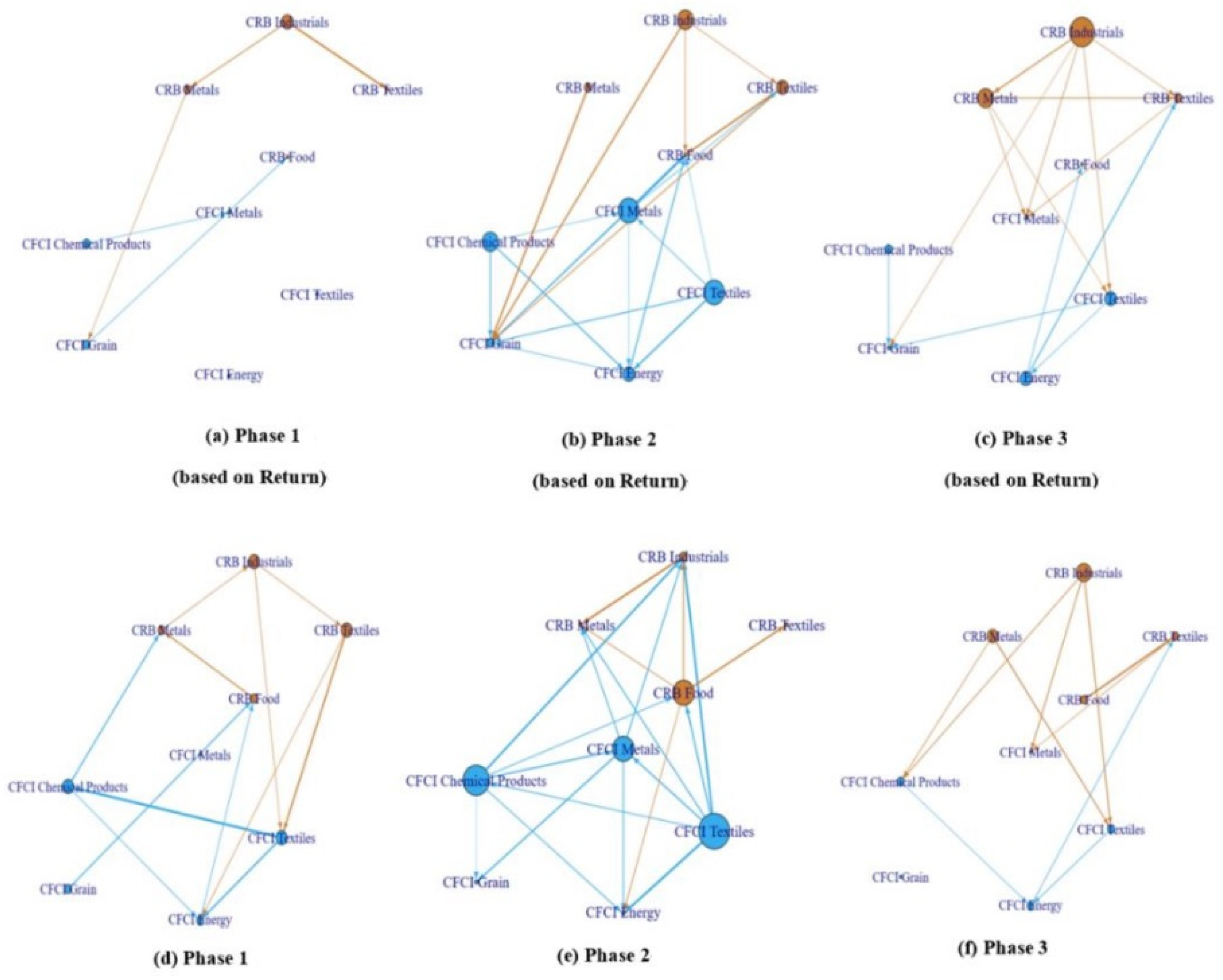
4.3. Dynamic Evolution of Risk Contagion during the COVID-19 Pandemic

In this section, we investigate the impact of the COVID-19 pandemic on China’s and foreign commodity markets and explore the dynamic evolution of risk contagion during this period. We compute the net volatility spillovers between commodities for Phase 1 (1 January 2019–30 November 2019), Phase 2 (1 December 2019–26 April 2020), and Phase 3 of the pandemic (27 April 2020–19 March 2021). The results are presented in Table 4. On 1 December 2019, The Lancet published the time of the first COVID-19 epidemic diagnosis; on 26 April 2020, the last confirmed case in Wuhan was eliminated, marking a success in China’s epidemic prevention and control.
As shown in Table 4, during Phase 1 of the pandemic (Panel A), the net volatility spillovers between the varieties were relatively small, and CRB Industrials and CFCI Chemical Products were the main exporters of the risk with TNSOUT reaching 8.62 and 13.86, respectively, based on the Return variable, while CFCI Metals, CRB Textiles, and CRB Energy were the main recipients of the risk with TNSOUT reaching −8.04, −6.98, and −6.58, respectively.
During Phase 2 (Panel B), in addition to the sharp increase in risk contagion among the Chinese varieties, the volatility spillovers from China’s to the foreign varieties also increased significantly. CFCI Textiles, CFCI Metals, and CFCI Chemical Products became the main exporters of the risk with TNSOUT reaching 17.99, 12.32, and 14.64, respectively (71.45, 25.54, and 36.99, respectively, based on the VaR). That is an increase of 18.63, 20.36, and 6.02, respectively, from Phase 1 (an increase of 63.11, 36.14, and 36.33, respectively, based on VaR). CRB Food and CFCI Grain became the net recipients of risk from almost all varieties with TNSOUT reaching −32.11 and −28.1, respectively, based on the Return variable. During Phase 2, the systemic risk was significantly intensified and China’s commodities became the main source of risk exporters in the global commodities market.
During Phase 3 of the pandemic (Panel C), the volatility spillover between Chinese varieties subsided significantly. However, TNSOUT of CRB Industrials reached 13.96 (33.41 based on the VaR variable), becoming the main source of risk contagion. The dynamic evolution of risk contagion under the impact of the COVID-19 pandemic is obvious.
Next, we draw the network topology of variance decompositions suggested by Diebold and Yilmaz [13] for the net volatility spillovers between China’s and foreign commodities during the three different periods. The results are presented in Figure 6. As can be seen from Figure 6, the volatility spillover network diagrams based on Return are qualitatively the same as those based on VaR. The lines of the network before the pandemic are relatively sparse, indicating that the risk contagion between commodity markets is not prevalent. We can see in Figure 6b,e that the number of blue lines in the network diagrams increases sharply, and the nodes of CFCI Textiles, CFCI Chemical products, and CFCI metals are larger in Phase 2 compared to those in Phase 1, suggesting that they are the main risk exporters during this period, consistent with the results from Table 4. Meanwhile, the increased incidence rate of workers, supply chain disruption, and economic embargo measures adopted by many countries had a strong negative impact on the global food supply. As a result, the price index of CRB Food plummeted from 324.26 to 275.91, which significantly accelerated the risk spillover of CRB Food. Therefore, the node of CRB Food in Figure 6e became significantly larger.
In Figure 6c,f, the nodes of the Chinese varieties are significantly reduced while the nodes of the foreign varieties become larger, and CRB Industrials and Metals became the main risk exporters during the third period. With the worldwide spread of the COVID-19 pandemic, the main sources of risk spillover were transferred from China’s commodities market to the foreign commodities market.

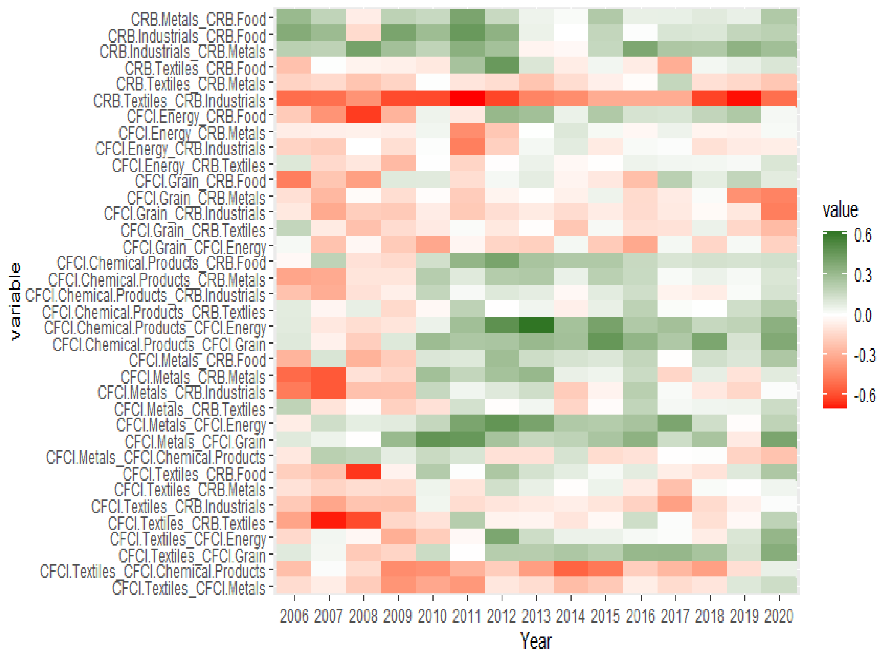
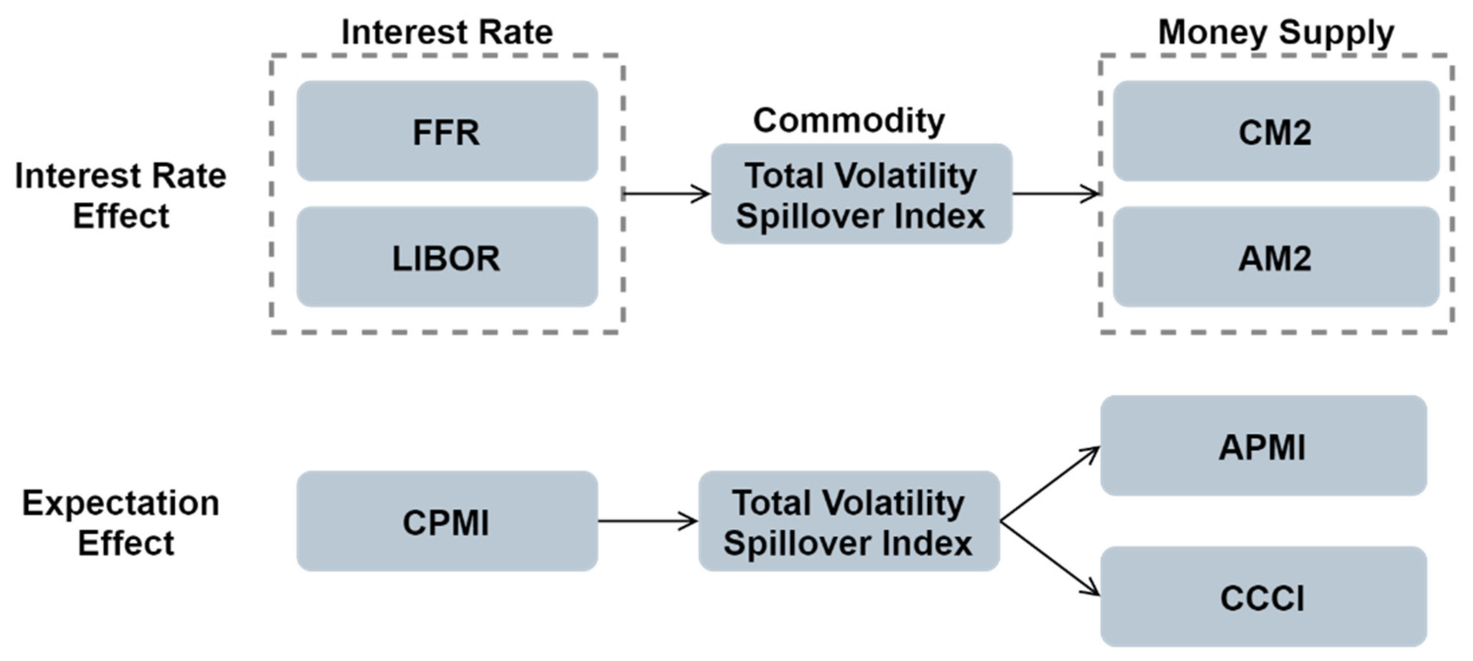
4.4. Analysis of the Risk Contagion Mechanism

To explore the reasons behind the evolution of the volatility spillovers in global commodity markets, the economic climate index, interest rate index, money supply, and consumer confidence index are considered in the analysis framework. The US manufacturing Purchasing Managers Index (APMI) and China PMI index (CPMI), respectively, are selected as the representative variables of the economic climate index; London InterBank Offered Rate (LIBOR), US Federal Fund Rates (FFR), and Shanghai Interbank Offered Rate (SHIBOR) are selected as representative variables of interest rates; China M2 growth rate (CM2) and US M2 growth rate (AM2) are selected as representative variables of money supply; China Consumer Confidence Index (CCCI) and the University of Michigan Consumer Confidence Index (ACCI) are selected as representative variables of the consumer confidence index.
Table 5 lists the relevant variables and their descriptive summaries. As can be seen from the table, the average values of the total volatility spillover index based on yield (Index–Return) and VaR (Index–VaR) are about 50, and the standard deviations are 7.21 and 9.47, respectively.
In addition, the traditional ADF method is used for the unit root test. In order to avoid sample deviation and low test efficacy, the DF–GLS method is also used to check the stationarity of the variables. The test results show that the variables above are stable after taking the first-order difference (still using the names of the original variables), except for the interest rate indexes, which are already stable in their original form.
Using the stable variables, the optimal bivariate VAR models are first used to estimate the interaction between variables to filter their linear interdependence. Then, the BDS test is performed in the residual series of the VAR models to test the nonlinear trend. As we can see from Table 6, most of the z-statistic results reject the null hypothesis of a linear relationship between variables. Thus, the linear causality test is not appropriate for these variables. The nonlinear Granger causality test [37] is conducted on the residual series using the bandwidth parameter, where ε = k · n−α, k ≈ 7, α = 0.28, and n is the length of time series. In this paper, we use ε = 1.6 for the monthly series and ε = 0.7 for the daily series. Combining with the BDS test results, we perform a nonlinear Granger causality test on these residual variables, which have nonlinear trends, and perform a linear Granger causality test on Index–Return (Index–VaR) and APMI. The results are presented in Table 7.
The Granger causality test results show that the results based on Return are generally consistent with those based on VaR, which further confirms the stability of the models and methods adopted in this paper. According to the causal relationship between interest rate and risk spillover, FFR and LIBOR have a one-way causal relationship on the spillover index; that is, the change of interest rate will affect the change of risk spillover in global bulk commodity markets. In addition, based on Return, there is a two-way causal relationship between them; that is, the change of risk spillover in the commodity markets also causes the change of interest rate levels of FFR and LIBOR. However, there is no Granger causality between the spillover index and SHIBOR. This conclusion shows that the changes of FFR and LIBOR have an impact on the commodities market and then cause the flow of international capital while SHIBOR does not produce such an effect.
Combined with the causality results in Table 7, the risk contagion mechanism diagram is summarized in Figure 7. We found that when the volatility spillover level of the commodity markets changes under the impact of interest rate level, it will have an impact on the money supply of China and the United States; that is, the path of risk contagion is “interest rate → commodities → money supply”. From the perspective of economic expectations, the causality of “China’s economic expectation → commodities → foreign economic expectation” shows that China’s economic expectations will have an impact on the risk contagion of commodity markets, and then affect the economic expectations of foreign manufacturing. This result may be related to China’s status as a world factory and manufacturing power. In addition, the risk contagion of commodity markets will also have an impact on the global consumer confidence index, with a one-way causal relationship of “commodity → consumer confidence”.

5. Conclusions

Using the network topological analysis of Diebold and Yilmaz [15], this paper examines the risk contagion effect between China’s and foreign commodity markets by constructing the volatility spillover index, focusing on the impact of the COVID-19 pandemic on the commodities market, and discussing the risk contagion mechanism through nonlinear Granger causality test.
It is found that energy, grain, and textiles are net risk recipients, and chemical products and metals are net exporters of risk contagion in China’s commodities market. The industrials sector has significant positive risk spillover to the metal and textile sectors in the international commodities market. On the interaction between China’s and foreign commodities, the international market usually transmits risk to China’s market. However, during the COVID-19 pandemic, with the sharp increase in the risk contagion among Chinese varieties, the metal and textile sectors became the main sources of the risk exportation to the international commodity markets. In the third period of the pandemic, the volatility spillover of Chinese varieties was significantly weakened; CRB industrials and metals became the main exporters of the risk.
The causality results show that the risk contagion in the commodities market follows three paths: “interest rate → commodities → money supply”, “China’s economic expectation → commodities → foreign economic expectation”, and “commodities → consumer confidence”.
These conclusions offer a detailed description of pathways of the risk contagion mechanism among global bulk commodities and have great implications for investors and policymakers in terms of understanding the transmission of volatility spillovers over to money supply, consumer confidence, and economic expectations of foreign manufacturing. Because of the risk spillover effects, the occurrence of the COVID-19 pandemic sharply increases the scale and intensity of risk contagion in the commodities market, and multiple pathways of risk contagion are formed in the global economic system. For investors, they should give close attention to the dynamic evolution of these events and adopt prudent investment strategies to avoid risk accumulation. Since the commodities market is located in a key position in the chains of risk contagion, policymakers should attempt to stabilize the supply and demand of bulk commodities and provide active guidance on the price expectation of bulk commodities to reduce the risk from shocks in external output. At the same time, our results show that interest rate and economic expectation are the important factors that can accelerate and amplify risk spillover in the commodities market and also cause a wider spread of risk. This also needs the attention of policymakers.
Just as in any market-specific and country-specific study, drawing any conclusion from the results in this study to other financial markets and countries should be done with care. Because of the limitation of space, this paper has not incorporated more economic and financial factors in the analytical framework of risk contagion between the commodity markets. The spillovers into other financial markets are also meaningful studies to help us realize the services provided by the financial sector to the global economy. Time–frequency connectedness and quantile spillovers approaches can also shed additional light on the risk contagion mechanism. These are all potential directions for future studies.

Author Contributions

H.S. carried out the conceptualization, methodology, writing—review and funding acquisition; Q.P. handled the data curation, formal analysis and writing—original draft preparation; L.Z. carried out the methodology and validation; P.N. handled the writing-editing and validation. All authors have read and agreed to the published version of the manuscript.

Funding

This research was funded by the National Natural Science Foundation of China (grant No. 61803331) and the Jiangsu Natural Science Foundation of China (BK20170515). The APC was funded by the National Natural Science Foundation of China (grant No. 61803331).

Informed Consent Statement

Not applicable.

Data Availability Statement

The data in this paper are all from the Wind database of China.

Conflicts of Interest

The authors declare no conflict of interest.

References

  1. Cavallo, E.; Galiani, S.; Noy, I.; Pantano, J. Catastrophic natural disasters and economic growth. Rev. Econ. Stat. 2013, 95, 1549–1561. [Google Scholar] [CrossRef] [Green Version]
  2. Worthington, A.; Valadkhani, A. Measuring the impact of natural disasters on capital markets: An empirical application using intervention analysis. Appl. Econ. 2004, 36, 2177–2186. [Google Scholar] [CrossRef] [Green Version]
  3. Zheng, Z.X.; Jiang, C.Y.; Xu, X.G.; Zhu, F.M. Monetary policy, commodity financialization and price fluctuation. Econ. Stud. 2020, 55, 76–91. [Google Scholar]
  4. Acerbi, C.; Tasche, D. On the coherence of expected shortfall. J. Bank. Financ. 2002, 26, S0378–S4266. [Google Scholar] [CrossRef] [Green Version]
  5. Hong, Y.M.; Cheng, S.W.; Liu, Y.H.; Wang, S.Y. Great risk spillover effect between China and the rest of the world. Econ. Q. 2004, 2, 703–726. [Google Scholar]
  6. Zhang, Q.; Wang, C.; Wang, K. Price risk measurement and analysis of livestock products market in China. Econ. Issues 2010, 3, 90–94. [Google Scholar] [CrossRef]
  7. Adrian, T.; Brunnermeier, M.K. CoVaR. Federal Reserve Bank of New York Staff Report; Princeton University: Princeton, NJ, USA, 2008; p. 348. [Google Scholar]
  8. Gao, G.H.; Pan, Y.L. Bank Systemic Risk Measurement—Analysis based on Dynamic CoVaR Method; Shanghai Jiao Tong University: Shanghai, China, 2011; Volume 45, pp. 1753–1759. [Google Scholar] [CrossRef]
  9. Mao, J.; Luo, M. Study on risk spillover effects between banking and securities industry—Analysis based on CoVaR model. New Financ. 2011, 5, 27–31. [Google Scholar]
  10. Li, S.W.; Wang, L.; Liu, X.X.; Zhang, J. Systemic risk research across banking and corporate departments. Theory Pract. Syst. Eng. 2020, 40, 2492–2504. [Google Scholar] [CrossRef]
  11. Baruník, J.; Křehlík, T. Measuring the frequency dynamics of financial connectedness and systemic risk. J. Financ. Econom. 2018, 16, 271–296. [Google Scholar] [CrossRef]
  12. Liu, Z.; Shi, X.; Zhai, P.; Wu, S.; Ding, Z.; Zhou, Y. Tail risk connectedness in the oil-stock nexus: Evidence from a novel quantile spillover approach. Resour. Policy 2021, 74, 102381. [Google Scholar] [CrossRef]
  13. Diebold, F.X.; Yilmaz, K. Measuring financial asset return and volatility spillovers, with application to global equity markets. Econ. J. 2009, 119, 159–171. [Google Scholar] [CrossRef] [Green Version]
  14. Diebold, F.X.; Yilmaz, K. Better to give than to receive: Predictive directional measurement of volatility spillovers. Int. J. Forecast. 2012, 28, 57–66. [Google Scholar] [CrossRef] [Green Version]
  15. Diebold, F.X.; Yilmaz, K. On the network topology of variance decompositions: Measuring the connectedness of financial firms. J. Econom. 2014, 182, 119–134. [Google Scholar] [CrossRef] [Green Version]
  16. McMillan, D.G.; Speight, A.E.H. Return and volatility spillovers in three euro exchange rates. J. Econ. Bus. 2009, 62, 79–93. [Google Scholar] [CrossRef]
  17. Cronin, D. The interaction between money and asset markets: A spillover index approach. J. Macroecon. 2014, 39, 185–202. [Google Scholar] [CrossRef]
  18. Fu, Q.; Zhang, Y. Risk spillover effect study of China financial system—Empirical analysis based on the overflow index. Macroecon. Res. 2015, 7, 45–51+117. [Google Scholar] [CrossRef]
  19. Yang, Z.H.; Zhou, Y. Global systematic financial risk overflow and external impact. Chin. Soc. Sci. 2018, 12, 69–90+200–201. [Google Scholar]
  20. Singh, A.; Kaur, P. A short note on information transmissions across US-BRIC equity markets: Evidence from volatility spillover index. J. Quant. Econ. 2017, 15, 197–208. [Google Scholar] [CrossRef]
  21. Zheng, J.H.; Fu, Y.F.; Tao, J. Analysis of the impact of COVID-19 epidemic on Consumer Economy. Consum. Econ. 2020, 36, 3–9. [Google Scholar]
  22. Wu, Z.Y.; Zhu, H.M.; Zhu, J.S. Impact of COVID-19 epidemic on financial operation and policy suggestions. Econ. Vert. 2020, 3, 1–6+137. [Google Scholar] [CrossRef]
  23. Fang, Y.; Yu, B.; Wang, W. Research on risk measurement and control of Chinese financial market under the influence of COVID-19 epidemic. J. Cent. Univ. Financ. Econ. 2020, 8, 116–128. [Google Scholar] [CrossRef]
  24. Yang, Z.H.; Chen, Y.T.; Zhang, P.M. Macroeconomic impact, financial risk transmission and governance response under major public emergencies. Manag. World 2020, 36, 13–35+7. [Google Scholar] [CrossRef]
  25. Fang, Y.; Jia, Y.Y. Risk prevention and control in global foreign exchange market under the impact of COVID-19 epidemic. Contemp. Econ. Sci. 2021, 43, 1–15. [Google Scholar]
  26. Kamdem, J.S.; Essomba, R.S.; Berinyuy, J.N. Deep learning models for forecasting and analyzing the implications of Covid-19 spread on some commodities markets volatilities. Chaos Solit. Fractals 2020, 140, 110215. [Google Scholar] [CrossRef]
  27. Dmytrów, K.; Landmesser, J.; Bieszk-Stolorz, B. The connections between COVID-19 and the energy commodities prices: Evidence through the Dynamic Time Warping method. Energies 2021, 14, 4024. [Google Scholar] [CrossRef]
  28. Elleby, C.; Domínguez, I.P.; Adenauer, M.; Genovese, G. Impacts of the COVID-19 pandemic on the global agricultural markets. Environ. Resour. Econ. 2020, 76, 1067–1079. [Google Scholar] [CrossRef]
  29. Erten, B.; Ocampo, J.A. The future of commodity prices and the pandemic driven global recession: Evidence from 150 years of data. World Dev. 2021, 137, 105164. [Google Scholar] [CrossRef]
  30. Bakas, D.; Triantafyllou, A. Commodity price volatility and the economic uncertainty of pandemics. Econ. Lett. 2020, 193, 109283. [Google Scholar] [CrossRef]
  31. Li, X.; Li, B.; Wei, G.; Bai, L.; Wei, Y.; Liang, C. Return connectedness among commodity and financial assets during the COVID-19 pandemic: Evidence from China and the US. Resour. Policy 2021, 73, 102166. [Google Scholar] [CrossRef]
  32. Umar, Z.; Gubareva, M.; Teplova, T. The impact of Covid-19 on commodity markets volatility: Analyzing time-frequency relations between commodity prices and coronavirus panic levels. Resour. Policy 2021, 73, 102164. [Google Scholar] [CrossRef]
  33. Borgards, O.; Czudaj, R.L.; Van Hoang, T.H. Price overreactions in the commodity futures market: An intraday analysis of the Covid-19 pandemic impact. Resour. Policy 2021, 71, 101966. [Google Scholar] [CrossRef]
  34. Koop, G.; Pesaran, M.H.; Potter, S.M. Impulse response analysis in non-linear multivariate models. J. Econom. 1996, 74, 119–147. [Google Scholar] [CrossRef]
  35. Pesaran, H.H.; Shin, Y. Generalized impulse response analysis in linear multivariate models. Econ. Lett. 1998, 58, 17–29. [Google Scholar] [CrossRef]
  36. Zhang, X.; Liu, L.; Li, L. Finalization and China’s macroeconomic fluctuations. Financ. Res. 2017, 1, 35–51. [Google Scholar]
  37. Diks, C.; Panchenko, V. A new statistic and practical guidelines for nonparametric Granger causality testing. J. Econ. Dyn. Control. 2006, 30, 1647–1669. [Google Scholar] [CrossRef] [Green Version]
Figure 1. The total volatility spillover of the rolling sample. Notes: (1) The top figure is based on the logarithmic yield and the bottom figure is based on VaR; the length of the forecast is 10 days and the rolling window is 200 days. (2) Event (1): In August 2008, the international financial crisis began to lose control, and many large financial institutions closed or were supervised by the government; Event (2): On 11 March 2011, a magnitude 9.0 earthquake and tsunami occurred in Japan; Event (3): On 10 February 2015, international metals prices plunged 7.2% during the flash crash of the stock markets; Event (4): In August 2015, a major stock market crash in China occurred; Event (5): In June 2016, UK Brexit referendum was approved; Event (6): On 31 August 2018, China’s domestic food prices increased by 25.2% daily; Event (7): In March 2020, the World Health Organization declared COVID-19 outbreak a pandemic.
Energies 15 02492 g001
Figure 2. The “OUT” total directional volatility spillover of the rolling sample.
Energies 15 02492 g002
Figure 3. The “IN” directional volatility spillover diagram of rolling samples.
Energies 15 02492 g003
Figure 4. The net volatility spillover diagram of rolling samples.
Energies 15 02492 g004
Figure 5. Thermal diagram of the directional volatility spillover between commodities. Note: Take the variable “A_B” as an example, if the color is green, A is the risk exporter while B is the risk recipient; if the color is red, B is the risk exporter and A is the risk recipient.
Energies 15 02492 g005
Figure 6. Net volatility spillover network diagrams for the three periods. Notes: (1) The larger the node, the greater the “out-degree” of the variety in risk contagion; (2) the orange line represents that the international variety is the risk exporter, and the blue line represents that the Chinese variety is the risk exporter; (3) return’s net volatility spillover network is based on the part where the net volatility spillover index is greater than 2; the net volatility spillover network diagram of VaR is based on the part where the net volatility spillover index is greater than 5; (4) Panels (a)–(c) are the network diagrams based on Return while (d)–(f) are based on VaR.
Energies 15 02492 g006
Figure 7. The risk contagion mechanism.
Energies 15 02492 g007
Table 1. Descriptive statistics of the logarithmic yields.
ChinaInternational
CFCI TextilesCFCI
Metals
CFCI Chemical ProductsCFCI
Grain
CFCI EnergyCRB TextilesCRB
Industrials
CRB
Metals
CRB
Food
Average−0.0080.015−0.0010.0200.0190.0070.0150.0290.014
Median 0.0110.0310.0270.0140.0420.0000.0180.0290.009
Maximum 14.5447.0189.66722.4578.1759.9344.96612.7883.782
Minimum −12.850−5.348−8.574−23.871−8.597−9.486−4.459−10.140−9.434
Standard deviation1.1061.2821.4761.0681.4760.5280.5241.0580.736
Skewness0.211−0.115−0.1471.564−0.3000.175−0.334−0.110−0.842
Kurtosis25.0805.6795.407179.5986.11868.31415.31120.90813.644
JB73,278 ***1086.6 ***883.2 ***4,687,304 ***1514.8 ***640,965 ***22,840 ***48,192 ***17,448 ***
ADF−42.3 ***−40.1 ***−39.6 ***−49.3 ***−41.3 ***−43.5 ***−38.6 ***−40.8 ***−39.5 ***
Notes: (1) *** indicates significance at 1%; (2) JB is Jarque–Bera test; (3) ADF is augmented Dickey–Fuller unit root test.
Table 2. Volatility spillover matrix between commodities.
VarietyCFCI TextilesCFCI
Metals
CFCI Chemical ProductsCFCI
Grain
CFCI
Energy
CRB TextilesCRB
Industrials
CRB
Metals
CRB
Food
IN
CFCI Textiles53.28.619.442.615.14.683.331.851.1946.8
CFCI Metals743.5616.922.6512.481.436.797.541.6356.44
CFCI Chemical Products15.7116.7643.013.1510.821.613.953.761.2356.99
CFCI Grain3.694.545.4576.213.210.891.961.532.5223.79
CFCI Energy5.0515.6513.432.3753.311.163.563.611.8746.69
CRB Textiles3.591.271.520.60.6169.9216.22.713.5930.08
CRB Industrials2.045.263.391.122.359.744230.643.4658
CRB Metals1.36.443.710.942.661.8334.1646.572.3953.43
CRB Food 1.041.421.492.270.874.055.653.8579.3720.63
OUT39.4359.9365.3415.7138.0925.3775.655.517.88392.85
Column Total92.63103.48108.3491.9391.495.29117.6102.0797.2543.70%
Notes: (1) Table 2 reports the volatility spillover matrix with a forecast period of 10 days, as shown in Equation (3); the ij-th element measures the contribution to the forecast error variance of variety i coming from shocks in variety j; (2) the i-th element in the column of “IN” indicates the total volatility spillover effect of other varieties on variety i measured from the perspective of total scale using Equation (5), and the j-th element in the row of “OUT” indicates the total volatility spillover effect of variety j on other markets measured from the perspective of total scale using Equation (6); the value in each row of the “IN” column is the sum of the off-diagonal elements of that row, likewise for the columns of the OUT row; (3) elements in the lower right corner measures the total effect of systemic volatility spillovers using Equation (4).
Table 3. Net volatility spillover matrix between commodities.
VarietyCFCI TextilesCFCI
Metals
CFCI Chemical ProductsCFCI
Grain
CFCI EnergyCRB TextilesCRB
Industrials
CRB
Metals
CRB
Food
TNSIN
CFCI Textiles01.63.73−1.080.051.091.290.550.157.38
CFCI Metals−1.600.16−1.89−3.170.161.531.10.21−3.5
CFCI Chemical Products−3.73−0.160−2.3−2.610.090.560.05−0.26−8.36
CFCI Grain1.081.892.300.840.290.840.590.258.08
CFCI Energy−0.053.172.61−0.8400.551.210.9518.6
CRB Textiles−1.09−0.16−0.09−0.29−0.5506.460.88−0.464.7
CRB Industrials−1.29−1.53−0.56−0.84−1.21−6.460−3.52−2.19−17.6
CRB Metals−0.55−1.1−0.05−0.59−0.95−0.883.520−1.46−2.06
CRB Food −0.15−0.210.26−0.25−10.462.191.4602.76
TNSOUT−7.383.58.36−8.08−8.6−4.717.62.06−2.760
Table 4. The net volatility spillover between commodities over the three periods of the pandemic.
Panel A: Phase 1.
Variety CFCI TextilesCFCI
Metals
CFCI Chemical ProductsCFCI
Grain
CFCI EnergyCRB TextilesCRB
Industrials
CRB
Metals
CRB
Food
TNSIN
CFCI TextilesVaR Return 0.00
0.00
−2.01
−1.57
−17.7
0.77
2.07
0.32
−12.93
−1.23
13.61
1.18
6.27
1.17
2.76
0.45
−0.41
−0.45
−8.34
0.64
CFCI MetalsVaR Return 2.01
1.57
0.00
0.00
9.67
2.38
−0.21
1.30
−1.99
0.35
1.93
0.34
1.00
0.92
−0.31
0.21
−1.50
0.97
10.6
8.04
CFCI Chemical ProductsVaR Return 17.70
−0.77
−9.67
−2.38
0.00
0.00
−0.33
−0.59
−6.58
−1.33
1.54
−1.47
0.14
−0.82
0.04
−1.69
−3.50
0.43
−0.66
−8.62
CFCI GrainVaR Return −2.07
−0.32
0.21
−1.30
0.33
0.59
0.00
0.00
−0.69
−1.31
−1.30
1.19
−1.02
0.24
3.88
2.79
−9.24
−2.84
−9.9
−0.96
CFCI EnergyVaR Return 12.93
1.23
1.99
−0.35
6.58
1.33
0.69
1.31
0.00
0.00
6.23
−0.13
3.76
1.16
−4.78
0.20
−6.13
1.83
21.27
6.58
CRB TextilesVaR Return −13.61
−1.18
−1.93
−0.34
−1.54
1.47
1.30
−1.19
−6.23
0.13
0.00
0.00
5.12
7.05
−3.71
1.58
−4.61
−0.54
−25.21
6.98
CRB IndustrialsVaR Return −6.27
−1.17
−1.00
−0.92
−0.14
0.82
1.02
−0.24
−3.76
−1.16
−5.12
−7.05
0.00
0.00
5.51
−3.96
0.84
−0.18
−8.92
−13.86
CRB MetalsVaR Return −2.76
−0.45
0.31
−0.21
−0.04
1.69
−3.88
−2.79
4.78
−0.20
3.71
−1.58
−5.51
3.96
0.00
0.00
9.39
0.53
6.00
0.95
CRB Food VaR Return 0.41
0.45
1.5
−0.97
3.5
−0.43
9.24
2.84
6.13
−1.83
4.61
0.54
−0.84
0.18
−9.39
−0.53
0.00
0.00
15.16
0.25
TNSOUTVaR Return 8.34
−0.64
−10.6
−8.04
0.66
8.62
9.90
0.96
−21.27
−6.58
25.21
−6.98
8.92
13.86
−6.00
−0.95
−15.16
−0.25
0.00
0.00
Panel B: Phase 2
Variety CFCI TextilesCFCI
Metals
CFCI Chemical ProductsCFCI
Grain
CFCI EnergyCRB TextilesCRB
Industrials
CRB
Metals
CRB
Food
TNSIN
CFCI TextilesVaR Return 0.00
0.00
−9.90
−3.23
−6.95
−1.25
−4.21
−4.06
−16.13
−6.37
0.90
−0.37
−16.08
1.12
−8.90
−0.40
−10.18
−2.33
−71.45
−17.99
CFCI MetalsVaR Return 9.90
3.23
0.00
0.00
3.66
2.28
−10.94
−4.40
−8.30
−1.99
−4.74
−2.74
−8.70
1.05
−8.21
0.02
1.79
−9.77
−25.54
−12.32
CFCI Chemical ProductsVaR Return 6.95
1.25
−3.66
−2.28
0.00
0.00
−3.13
−4.43
−7.56
−4.87
1.44
−0.90
−14.77
−0.90
−9.79
−1.17
−6.47
−1.34
−36.99
−14.64
CFCI GrainVaR Return 4.21
4.06
10.94
4.40
3.13
4.43
0.00
0.00
−0.20
2.93
0.70
3.58
4.89
5.62
4.27
6.43
1.08
−3.35
29.02
28.10
CFCI EnergyVaR Return 16.13
6.37
8.30
1.99
7.56
4.87
0.20
−2.93
0.00
0.00
−0.98
0.64
2.29
0.58
−0.71
−0.34
5.92
−4.72
38.71
6.46
CRB TextilesVaR Return −0.9
0.37
4.74
2.74
−1.44
0.90
−0.70
−3.58
0.98
−0.64
0.00
0.00
2.13
2.59
−0.91
1.13
11.62
−6.57
15.52
−3.06
CRB IndustrialsVaR Return 16.08
−0.02
8.70
−1.05
14.77
0.90
−4.89
−5.62
−2.29
−0.58
−2.13
−2.59
0.00
0.00
−13.85
0.44
8.66
−2.92
25.05
−11.44
CRB MetalsVaR Return 8.90
0.40
8.21
−0.02
9.79
1.17
−4.27
−6.43
0.71
0.34
0.91
−1.13
13.85
−0.44
0.00
0.00
5.70
−1.11
43.8
−7.22
CRB Food VaR Return 10.18
2.33
−1.79
9.77
6.47
1.34
−1.08
3.35
−5.92
4.72
−11.62
6.57
−8.66
2.92
−5.70
1.11
0.00
0.00
−18.12
32.11
TNSOUTVaR Return 71.45
17.99
25.54
12.32
36.99
14.64
−29.02
−28.10
−38.71
−6.46
−15.52
3.06
−25.05
11.44
−43.8 7.2218.12
−32.11
0.00
0.00
Panel C: Phase 3
Variety CFCI TextilesCFCI
Metals
CFCI Chemical ProductsCFCI
Grain
CFCI EnergyCRB TextilesCRB
Industrials
CRB
Metals
CRB
Food
TNSIN
CFCI TextilesVaR Return 0.00
0.00
4.17
−1.26
2.86
0.57
−0.89
−2.75
−6.36
−2.46
1.03
−0.38
10.14
2.54
9.66
2.04
−4.53
1.00
16.08
−0.70
CFCI MetalsVaR Return −4.17
1.26
0.00
0.00
−4.77
0.69
−4.67
−1.75
−3.19
0.36
5.54
2.29
8.25
3.01
0.87
2.76
−2.19
−1.07
−4.33
7.55
CFCI Chemical ProductsVaR Return−2.86
−0.57
4.77
−0.69
0.00
0.00
−0.67
−2.99
−5.64
−1.24
0.23
−0.98
7.69
0.63
6.95
0.78
−4.05
0.15
6.42
−4.91
CFCI GrainVaR Return0.89
2.75
4.67
1.75
0.67
2.99
0.00
0.00
1.02
1.82
1.25
0.54
−2.44
2.12
−1.01
0.63
1.56
1.41
6.61
14.01
CFCI EnergyVaR Return6.36
2.46
3.19
−0.36
5.64
1.24
−1.02
−1.82
0.00
0.00
−6.16
−4.82
0.84
−0.90
2.01
−0.73
1.84
−2.68
12.7
−7.61
CRB TextilesVaR Return−1.03
0.38
−5.54
−2.29
−0.23
0.98
−1.25
−0.52
6.16
4.82
0.00
0.00
1.16
2.44
−4.55
3.40
14.41
−0.44
9.13
8.75
CRB IndustrialsVaR Return−10.14
−2.54
−8.25
−3.10
−7.69
−0.63
2.44
−2.12
−0.84
0.90
−1.16
−2.44
0.00
0.00
−4.00
−4.59
−3.77
0.47
−33.41
−13.96
CRB MetalsVaR Return−9.66
−2.04
−0.87
−2.76
−6.95
−0.78
1.01
−0.63
−2.01
0.73
4.55
−3.40
4.00
4.59
0.00
0.00
−2.84
−0.38
−12.77
−4.67
CRB Food VaR Return4.53
−1.00
2.19
1.07
4.05
−0.15
−1.56
−1.41
−1.84
2.68
−14.41
0.44
3.77
−0.47
2.84
0.38
0.00
0.00
−0.43
1.54
TNSOUTVaR Return−16.08
0.70
4.33
−7.55
−6.42
4.91
−6.61
−14.01
−12.7
7.61
−9.13
−8.75
33.41
13.96
12.77
4.67
0.43
−1.54
0.00
0.00
Table 5. Descriptive statistics of the related variables.
Index
–Return
Index
–VaR
LIBORFFRSHIBORAM2CM2CPMIAPMICCCIACCI
Average51.0749.491.071.022.330.070.1450.4752.98109.6882.45
Median 49.1546.910.240.182.280.060.1350.5052.90107.8082.50
Maximum 67.6577.466.885.4113.830.270.3052.3064.70127.00101.40
Minimum 38.8434.370.050.040.680.020.0842.5033.1097.0055.30
Standard deviation7.219.471.501.460.910.050.051.215.228.1512.33
Skewness0.491.041.791.812.072.681.17−3.36−1.200.59−0.30
Kurtosis2.093.505.245.3616.9010.044.3422.105.602.192.05
Table 6. BDS test on the residual series of the bivariate VAR models.
VariablesBased on Index–Return
z-Statistic
Based on Index–Risk
z-Statistic
LIBOR48.65 ***5.82 ***48.72 ***15.13 ***
FFR33.83 ***5.77 ***32.48 ***15.26 ***
SHIBOR30.7 ***5.68 ***30.62 ***15.37 ***
AM23.92 ***5.30 ***4.96 ***2.20 **
CM22.01 **5.06 ***1.382.11 **
CPMI7.89 ***1.9 *7.59 ***1.72 *
APMI1.521.651.9 *1.56
CCCI0.194.84 ***−0.312.19 **
ACCI0.174.69 ***−0.112.09 **
Notes: (1) The optimal lag order of each bivariate VAR model is determined based on AIC and SIC information criteria; (2) “based on Index–Return” means the bivariate VAR model is constructed by Index–Return and other variables, and the numbers are the z-statistics of the residual series; (3) ***, **, and * indicate the rejection of the hypothesis of “linear relationship “ at the significance level of 1%, 5%, and 10%, respectively.
Table 7. Causality test of risk contagion.
Interest Rate and Risk SpilloverMonetary Supply and Risk SpilloverEconomic Expectations and Risk SpilloverInvestor Confidence and Risk Spillover
Index(Return) Energies 15 02492 i001FFRIndex(Return) Energies 15 02492 i002CM2Index(Return) Energies 15 02492 i003APMIIndex(Return) Energies 15 02492 i002ACCI
Index(VaR) Energies 15 02492 i004FFRIndex(VaR) Energies 15 02492 i003CM2Index(VaR) Energies 15 02492 i002APMIIndex(VaR) Energies 15 02492 i003ACCI
Index(Return) Energies 15 02492 i005LIBORIndex(Return) Energies 15 02492 i006AM2Index(Return) Energies 15 02492 i005CPMIIndex(Return) Energies 15 02492 i006CCCI
Index(VaR) Energies 15 02492 i007 LIBORIndex(VaR) Energies 15 02492 i002AM2Index(VaR) Energies 15 02492 i001CPMIIndex(VaR) Energies 15 02492 i002CCCI
Note: ***, **, and * indicate the rejection of the hypothesis that “there is no Granger causality” at the significance level of 1%, 5%, and 10%, respectively.
Publisher’s Note: MDPI stays neutral with regard to jurisdictional claims in published maps and institutional affiliations.

