
Optimal Placement of Capacitors in Radial Distribution Grids via Enhanced Modified Particle Swarm Optimization


Abstract
:1. Introduction
- Review of analytical, heuristic and their combinational methods reported in the literature for tackling optimal placement and sizing of the capacitor problem.
- A novel modified evolutionary algorithm is executed for reactive power planning in a radial distribution system.
- Analytical and heuristic combinational algorithms are applied on three IEEE distribution systems.
- Three objectives for intensification of annual net savings are achieved while considering system constraints.
2. OPSC Problem Formulation
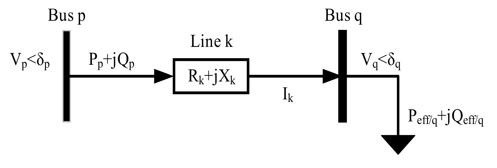
2.1. Power Flow Formulation
2.2. Objective Function
2.3. System Constraints
2.3.1. Voltage Limitation
2.3.2. Reactive Injection Limitation
2.3.3. Maximum Reactive Power Limitation
3. Methodology
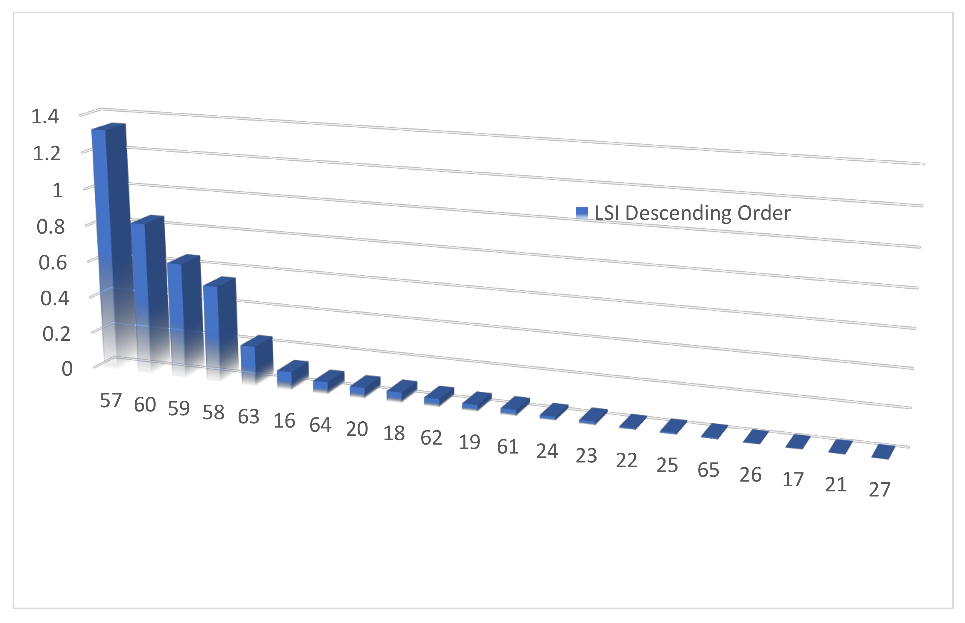
3.1. Loss Sensitivity Factor
3.1.1. Power Loss Indexing
3.1.2. LSF Ranking
3.1.3. Operating Voltage Normalization
3.1.4. Selection of Candidate Buses
3.2. Fixed and Switched Capacitors
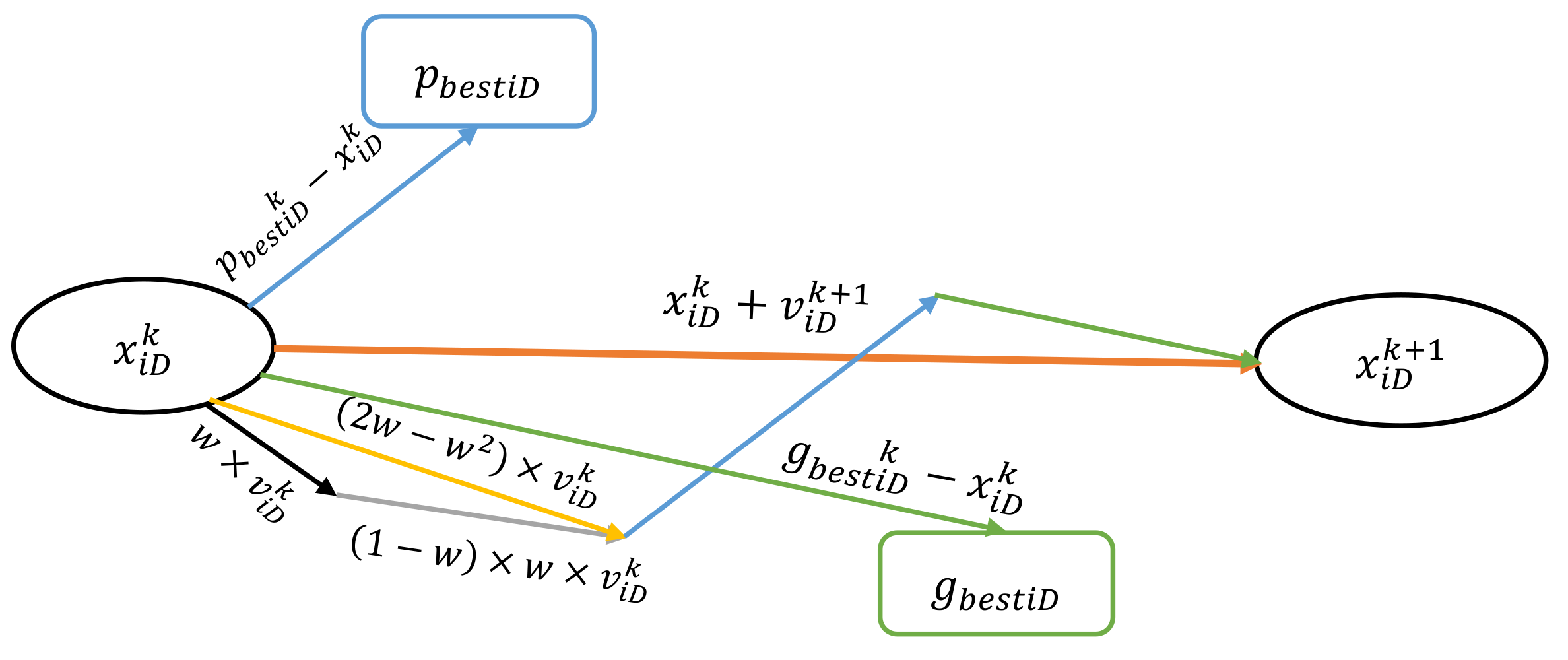
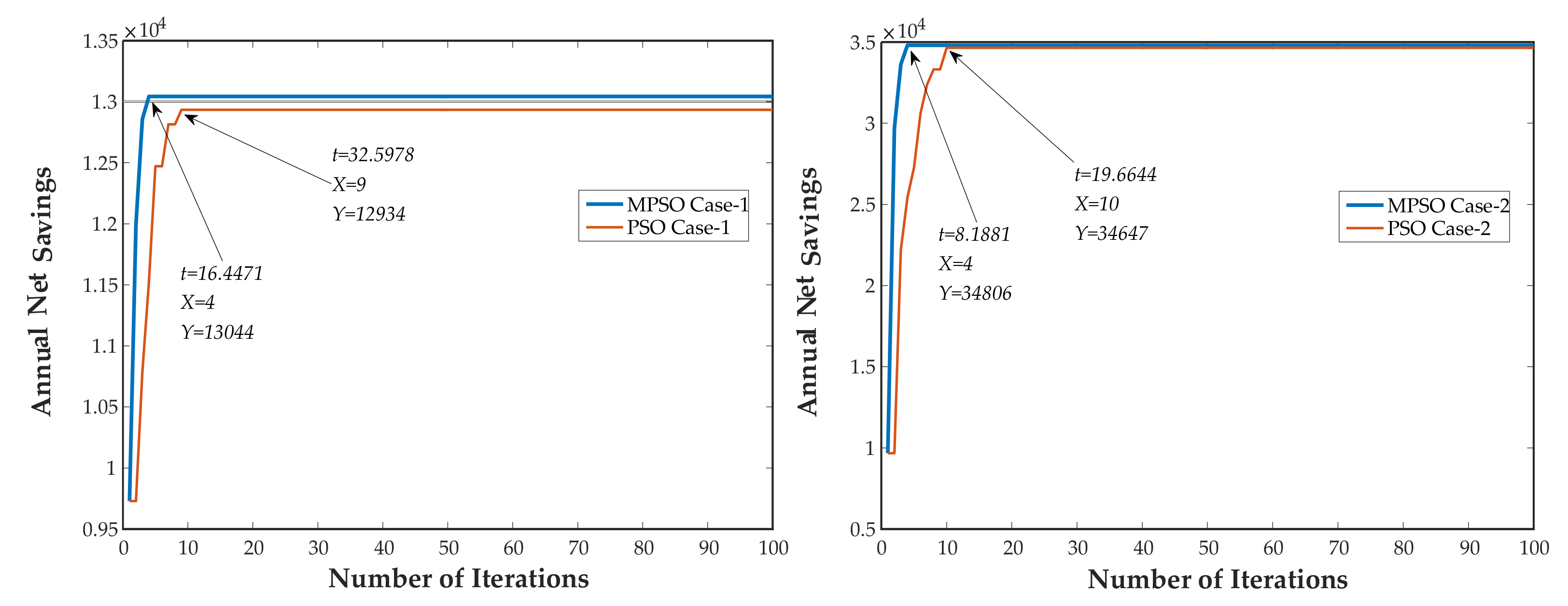
3.3. Novel Modified Particle Swarm Optimization

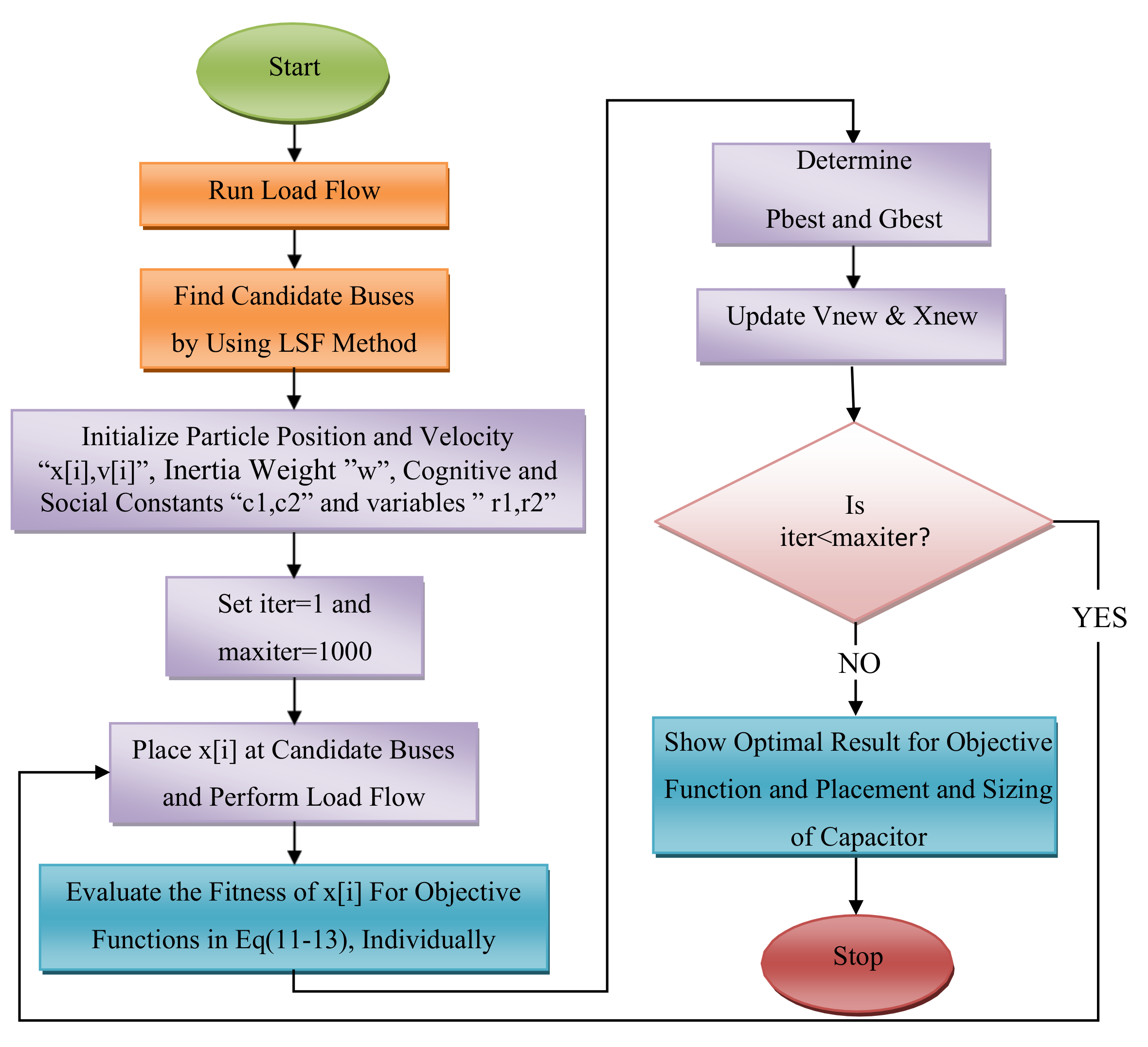
4. Execution of MPSO for OPSC
- Step 1
- Perform load flow to evaluate the initial state of the RDG in terms of power losses, total annual cost, minimum voltage.
- Step 2
- Use loss sensitivity method to highlight the potential buses for the optimal capacitor placement.
- Step 3
- Initialize random set of solutions; particle velocity, particle position, cognitive, social components, and random variables.
- Step 4
- Set maximum iteration limit.
- Step 5
- Check whether generated solution is satisfying the constraints; install capacitors on optimal buses while satisfying the (14)–(16).
- Step 6
- Evaluate the fitness of the solution in each iteration for (11)–(13); total annual cost.
- Step 7
- Generate new set of solutions using (21) and (22); update particle velocity and particle position.
- Step 8
- Stop the algorithm and display the result when it reached to maximum iteration or optimal solution is achieved; power losses reduction, total annual cost reduction, improvement of voltage profile, enhancement of annual net saving.
5. Results and Discussion
5.1. Statistical Analysis

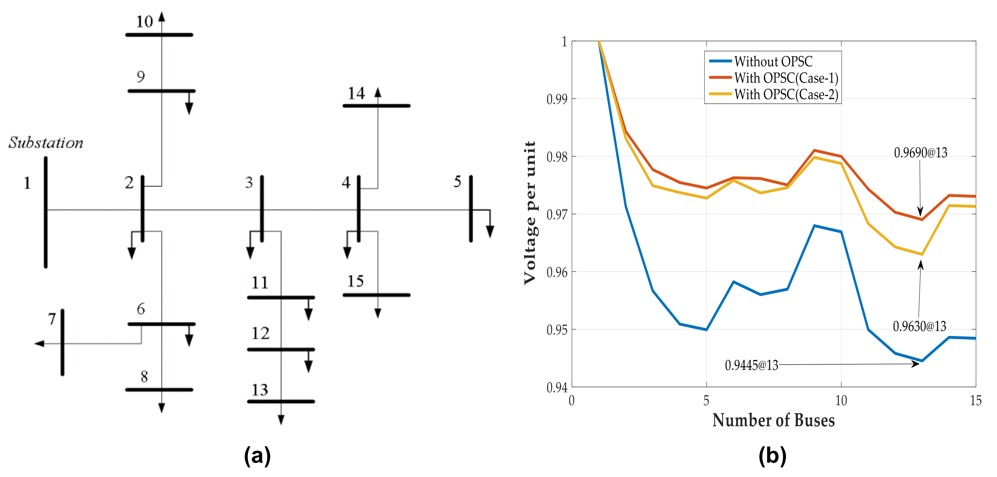
5.2. IEEE 15 Bus RDG


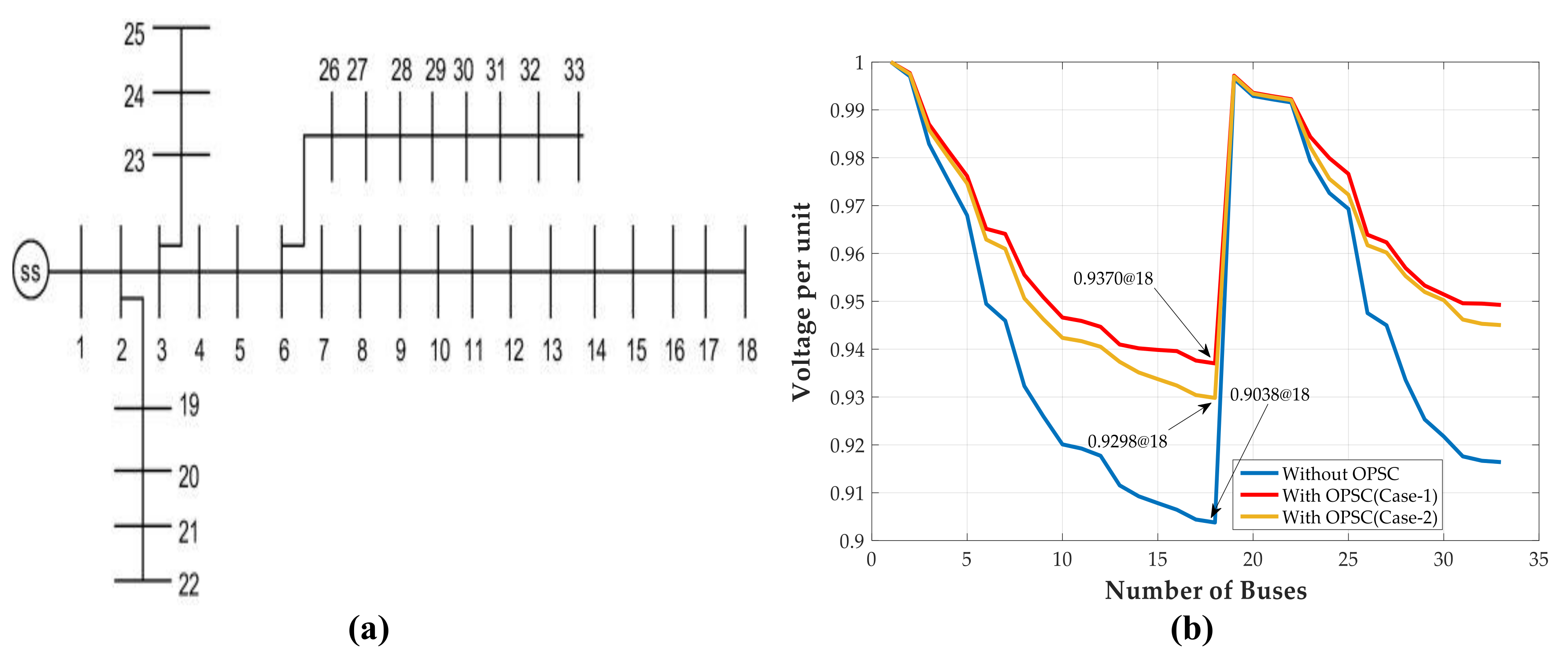
5.3. IEEE 33 Bus RDG


5.4. IEEE 69 Bus RDG

6. Conclusions
Author Contributions
Funding
Institutional Review Board Statement
Informed Consent Statement
Data Availability Statement
Acknowledgments
Conflicts of Interest
Abbreviations
| RDG | Radial distribution system |
| OPSC | Optimal placement and sizing of capacitors |
| LSF | Loss sensitivity factor |
| VSI | Voltage stability index |
| PLI | Power loss index |
| MAPSO | Multi-agent particle swarm optimization |
| TSM | Two-stage method |
| dPSO | Discrete particle swarm optimization |
| DE | Differential evolution algorithm |
| IHA | Improved harmony algorithm |
| FPA | Flower pollination algorithm |
| MPSO | Modified particle swarm optimization |
| IP | Interior point |
| SA | Simulated annealing |
| MMS | Modified monkey search |
| LS | Locust search algorithm |
| Fuzzy-GA | Fuzzy genetic algorithm |
Appendix A

| Capacitor Index (qc) | Capacitor Size (kVAr) Qc=Q(qc) | Reactive Power Cost ($/KVAr) | Capacitor Index (qc) | Capacitor Size (kVAr) Qc=Q(qc) | Reactive Power Cost ($/KVAr) |
|---|---|---|---|---|---|
| 1 | 150 | 0.500 | 11 | 1650 | 0.193 |
| 2 | 300 | 0.350 | 12 | 1800 | 0.187 |
| 3 | 450 | 0.253 | 13 | 1950 | 0.211 |
| 4 | 600 | 0.220 | 14 | 2100 | 0.176 |
| 5 | 750 | 0.276 | 15 | 2250 | 0.197 |
| 6 | 900 | 0.183 | 16 | 2400 | 0.170 |
| 7 | 1050 | 0.228 | 17 | 2550 | 0.189 |
| 8 | 1200 | 0.170 | 18 | 2700 | 0.187 |
| 9 | 1350 | 0.207 | 19 | 2850 | 0.183 |
| 10 | 1500 | 0.201 | 20 | 3000 | 0.180 |
| Line No. | From Bus | To Bus | Line Resistance R () | Line Reactance X () | Active Load Power (kW) | Reactive Load Power (kVAr) |
|---|---|---|---|---|---|---|
| 1 | 1 | 2 | 1.353090 | 1.323490 | 44.10 | 44.99 |
| 2 | 2 | 3 | 1.170240 | 1.144640 | 70.00 | 71.40 |
| 3 | 3 | 4 | 0.841110 | 0.822710 | 140.00 | 142.82 |
| 4 | 4 | 5 | 1.523480 | 1.027600 | 44.10 | 44.99 |
| 5 | 2 | 9 | 2.013170 | 1.357900 | 140.00 | 142.82 |
| 6 | 9 | 10 | 1.686710 | 1.137700 | 140.00 | 142.82 |
| 7 | 2 | 6 | 2.557270 | 1.724900 | 70.00 | 71.40 |
| 8 | 6 | 7 | 1.088200 | 0.734000 | 70.00 | 71.40 |
| 9 | 6 | 8 | 1.251430 | 0.844100 | 44.10 | 44.99 |
| 10 | 3 | 11 | 1.795530 | 1.211100 | 140.00 | 142.82 |
| 11 | 11 | 12 | 2.448450 | 1.651500 | 70.00 | 71.40 |
| 12 | 12 | 13 | 2.013170 | 1.357900 | 44.10 | 44.99 |
| 13 | 4 | 14 | 2.230810 | 1.504700 | 70.00 | 71.40 |
| 14 | 4 | 15 | 1.197020 | 0.807400 | 140.00 | 142.82 |
| Line No. | From Bus | To Bus | Line Resistance R () | Line Reactance X () | Active Load Power (kW) | Reactive Load Power (kVAr) |
|---|---|---|---|---|---|---|
| 1 | 1 | 2 | 0.09220 | 0.04770 | 100.00 | 60.00 |
| 2 | 2 | 3 | 0.49300 | 0.25110 | 90.00 | 40.00 |
| 3 | 3 | 4 | 0.36600 | 0.18640 | 120.00 | 80.00 |
| 4 | 4 | 5 | 0.38110 | 0.19410 | 60.00 | 30.00 |
| 5 | 5 | 6 | 0.81900 | 0.70700 | 60.00 | 20.00 |
| 6 | 6 | 7 | 0.18720 | 0.61880 | 200.00 | 100.00 |
| 7 | 7 | 8 | 1.71140 | 1.23510 | 200.00 | 100.00 |
| 8 | 8 | 9 | 1.03000 | 0.74000 | 60.00 | 20.00 |
| 9 | 9 | 10 | 1.04000 | 0.74000 | 60.00 | 20.00 |
| 10 | 10 | 11 | 0.19660 | 0.06500 | 45.00 | 30.00 |
| 11 | 11 | 12 | 0.37440 | 0.12380 | 60.00 | 35.00 |
| 12 | 12 | 13 | 1.46800 | 1.15500 | 60.00 | 35.00 |
| 13 | 13 | 14 | 0.54160 | 0.71290 | 120.00 | 80.00 |
| 14 | 14 | 15 | 0.59100 | 0.52600 | 60.00 | 10.00 |
| 15 | 15 | 16 | 0.74630 | 0.54500 | 60.00 | 20.00 |
| 16 | 16 | 17 | 1.28900 | 1.72100 | 60.00 | 20.00 |
| 17 | 17 | 18 | 0.73200 | 0.57400 | 90.00 | 40.00 |
| 18 | 2 | 19 | 0.16400 | 0.15650 | 90.00 | 40.00 |
| 19 | 19 | 20 | 1.50420 | 1.35540 | 90.00 | 40.00 |
| 20 | 20 | 21 | 0.40950 | 0.47840 | 90.00 | 40.00 |
| 21 | 21 | 22 | 0.70890 | 0.93730 | 90.00 | 40.00 |
| 22 | 3 | 23 | 0.45120 | 0.30830 | 90.00 | 50.00 |
| 23 | 23 | 24 | 0.89800 | 0.70910 | 420.00 | 200.00 |
| 24 | 24 | 25 | 0.89600 | 0.70110 | 420.00 | 200.00 |
| 25 | 6 | 26 | 0.20300 | 0.10340 | 60.00 | 25.00 |
| 26 | 26 | 27 | 0.28420 | 0.14470 | 60.00 | 25.00 |
| 27 | 27 | 28 | 1.05900 | 0.93370 | 60.00 | 20.00 |
| 28 | 28 | 29 | 0.80420 | 0.70060 | 120.00 | 70.00 |
| 29 | 29 | 30 | 0.50750 | 0.25850 | 200.00 | 600.00 |
| 30 | 30 | 31 | 0.97440 | 0.96300 | 150.00 | 70.00 |
| 31 | 31 | 32 | 0.31050 | 0.36190 | 210.00 | 100.00 |
| 32 | 32 | 33 | 0.34100 | 0.53020 | 60.00 | 40.00 |
| Line No. | From Bus | To Bus | Line Resistance R () | Line Reactance X () | Active Load Power (kW) | Reactive Load Power (kVAr) |
|---|---|---|---|---|---|---|
| 1 | 1 | 2 | 0.0005 | 0.0012 | 0.00 | 0.00 |
| 2 | 2 | 3 | 0.0005 | 0.0012 | 0.00 | 0.00 |
| 3 | 3 | 4 | 0.0015 | 0.0036 | 0.00 | 0.00 |
| 4 | 4 | 5 | 0.0251 | 0.0294 | 0.00 | 0.00 |
| 5 | 5 | 6 | 0.3660 | 0.1864 | 2.60 | 2.20 |
| 6 | 6 | 7 | 0.3810 | 0.1941 | 40.40 | 30.00 |
| 7 | 7 | 8 | 0.0922 | 0.0470 | 75.00 | 54.00 |
| 8 | 8 | 9 | 0.0493 | 0.0251 | 30.00 | 22.00 |
| 9 | 9 | 10 | 0.8190 | 0.2707 | 28.00 | 19.00 |
| 10 | 10 | 11 | 0.1872 | 0.0619 | 145.00 | 104.00 |
| 11 | 11 | 12 | 0.7114 | 0.2351 | 145.00 | 104.00 |
| 12 | 12 | 13 | 1.0300 | 0.3400 | 8.00 | 5.00 |
| 13 | 13 | 14 | 1.0440 | 0.3400 | 8.00 | 5.00 |
| 14 | 14 | 15 | 1.0580 | 0.3496 | 0.00 | 0.00 |
| 15 | 15 | 16 | 0.1966 | 0.0650 | 45.00 | 30.00 |
| 16 | 16 | 17 | 0.3744 | 0.1238 | 60.00 | 35.00 |
| 17 | 17 | 18 | 0.0047 | 0.0016 | 60.00 | 35.00 |
| 18 | 18 | 19 | 0.3276 | 0.1083 | 0.00 | 0.00 |
| 19 | 19 | 20 | 0.2106 | 0.0690 | 1.00 | 0.60 |
| 20 | 20 | 21 | 0.3416 | 0.1129 | 114.00 | 81.00 |
| 21 | 21 | 22 | 0.0140 | 0.0046 | 5.00 | 3.50 |
| 22 | 22 | 23 | 0.1591 | 0.0526 | 0.00 | 0.00 |
| 23 | 23 | 24 | 0.3463 | 0.1145 | 28.00 | 20.00 |
| 24 | 24 | 25 | 0.7488 | 0.2475 | 0.00 | 0.00 |
| 25 | 25 | 26 | 0.3089 | 0.1021 | 14.00 | 10.00 |
| 26 | 26 | 27 | 0.1732 | 0.0572 | 14.00 | 10.00 |
| 27 | 3 | 28 | 0.0044 | 0.0108 | 26.00 | 18.60 |
| 28 | 28 | 29 | 0.0640 | 0.1565 | 26.00 | 18.60 |
| 29 | 29 | 30 | 0.3978 | 0.1315 | 0.00 | 0.00 |
| 30 | 30 | 31 | 0.0702 | 0.0232 | 0.00 | 0.00 |
| 31 | 31 | 32 | 0.3510 | 0.1160 | 0.00 | 0.00 |
| 32 | 32 | 33 | 0.8390 | 0.2816 | 14.00 | 10.00 |
| 33 | 33 | 34 | 1.7080 | 0.5646 | 19.50 | 14.00 |
| 34 | 34 | 35 | 1.4740 | 0.4873 | 6.00 | 4.00 |
| 35 | 3 | 36 | 0.0044 | 0.0108 | 26.00 | 18.55 |
| 36 | 36 | 37 | 0.0640 | 0.1565 | 26.00 | 18.55 |
| 37 | 37 | 38 | 0.1053 | 0.1230 | 0.00 | 0.00 |
| 38 | 38 | 39 | 0.0304 | 0.0355 | 24.00 | 17.00 |
| 39 | 39 | 40 | 0.0018 | 0.0021 | 24.00 | 17.00 |
| 40 | 40 | 41 | 0.7283 | 0.8509 | 1.20 | 1.00 |
| 41 | 41 | 42 | 0.3100 | 0.3623 | 0.00 | 0.00 |
| 42 | 42 | 43 | 0.0410 | 0.0478 | 6.00 | 4.30 |
| 43 | 43 | 44 | 0.0092 | 0.0116 | 0.00 | 0.00 |
| 44 | 44 | 45 | 0.1089 | 0.1373 | 39.22 | 26.30 |
| 45 | 45 | 46 | 0.0009 | 0.0012 | 39.22 | 26.30 |
| 46 | 4 | 47 | 0.0034 | 0.0084 | 0.00 | 0.00 |
| 47 | 47 | 48 | 0.0851 | 0.2083 | 79.00 | 56.40 |
| 48 | 48 | 49 | 0.2898 | 0.7091 | 384.70 | 274.50 |
| 49 | 49 | 50 | 0.0822 | 0.2011 | 384.70 | 274.50 |
| 50 | 8 | 51 | 0.0928 | 0.0473 | 40.50 | 28.30 |
| 51 | 51 | 52 | 0.3319 | 0.1140 | 3.60 | 2.70 |
| 52 | 9 | 53 | 0.1740 | 0.0886 | 4.35 | 3.50 |
| 53 | 53 | 54 | 0.2030 | 0.1034 | 26.40 | 19.00 |
| 54 | 54 | 55 | 0.2842 | 0.1447 | 24.00 | 17.20 |
| 55 | 55 | 56 | 0.2813 | 0.1433 | 0.00 | 0.00 |
| 56 | 56 | 57 | 1.5900 | 0.5337 | 0.00 | 0.00 |
| 57 | 57 | 58 | 0.7837 | 0.2630 | 0.00 | 0.00 |
| 58 | 58 | 59 | 0.3042 | 0.1006 | 100.00 | 72.00 |
| 59 | 59 | 60 | 0.3861 | 0.1172 | 0.00 | 0.00 |
| 60 | 60 | 61 | 0.5075 | 0.2585 | 1244.00 | 888.00 |
| 61 | 61 | 62 | 0.0974 | 0.0496 | 32.00 | 23.00 |
| 62 | 62 | 63 | 0.1450 | 0.0738 | 0.00 | 0.00 |
| 63 | 63 | 64 | 0.7105 | 0.3619 | 227.00 | 162.00 |
| 64 | 64 | 65 | 1.0410 | 0.5302 | 59.00 | 42.00 |
| 65 | 11 | 66 | 0.2012 | 0.0611 | 18.00 | 13.00 |
| 66 | 66 | 67 | 0.0047 | 0.0014 | 18.00 | 13.00 |
| 67 | 12 | 68 | 0.7394 | 0.2444 | 28.00 | 20.00 |
| 68 | 68 | 69 | 0.0047 | 0.0016 | 28.00 | 20.00 |


References
- Soma, G.G. Optimal Sizing and Placement of Capacitor Banks in Distribution Networks Using a Genetic Algorithm. Electricity 2021, 2, 187–204. [Google Scholar] [CrossRef]
- Stanelyte, D. Review of voltage and reactive power control algorithms in electrical distribution networks. Energies 2020, 13, 58. [Google Scholar] [CrossRef] [Green Version]
- Gampa, S.R. Optimum placement of shunt capacitors in a radial distribution system for substation power factor improvement using fuzzy GA method. Int. J. Electr. Power Energy Syst. 2016, 77, 314–326. [Google Scholar] [CrossRef]
- Kola Sampangi, S. Optimal capacitor allocation in distribution networks for minimization of power loss and overall cost using water cycle algorithm and grey wolf optimizer. Int. Trans. Electr. Energy Syst. 2020, 30, e12320. [Google Scholar] [CrossRef]
- Elsayed, A.M. Distribution system performance enhancement (Egyptian distribution system real case study. Int. Trans. Electr. Energy Syst. 2018, 28, e2545. [Google Scholar] [CrossRef]
- Abul’Wafa, A.R. Ant-lion optimizer-based multi-objective optimal simultaneous allocation of distributed generations and synchronous condensers in distribution networks. Int. Trans. Electr. Energy Syst. 2019, 29, e2755. [Google Scholar] [CrossRef]
- Al-Jubori, W.K.S.; Hussain, A.N. Optimum reactive power compensation for distribution system using dolphin algorithm considering different load models. Int. J. Electr. Comput. Eng. 2020, 10, 5032. [Google Scholar]
- Sambaiah, K.S. Optimal allocation of renewable distributed generation and capacitor banks in distribution systems using Salp Swarm algorithm. Int. J. Renew. Energy Res. 2019, 9, 96–107. [Google Scholar]
- Tamilselvan, V. Optimal capacitor placement in radial distribution systems using flower pollination algorithm. Alex. Eng. J. 2018, 57, 2775–2786. [Google Scholar] [CrossRef]
- Duong, T.L. Determining optimal location and size of capacitors in radial distribution networks using moth swarm algorithm. Int. J. Electr. Comput. Eng. 2020, 10, 5032. [Google Scholar] [CrossRef]
- Da Silva, J. FPAES: A Hybrid Approach for the Optimal Placement and Sizing of Reactive Compensation in Distribution Grids. Energies 2020, 13, 6409. [Google Scholar] [CrossRef]
- Askarzadeh, A. Capacitor placement in distribution systems for power loss reduction and voltage improvement: A new methodology. IET Gener. Transm. Distrib. 2016, 10, 3631–3638. [Google Scholar] [CrossRef]
- Prakash, D.B. Optimal siting of capacitors in radial distribution network using whale optimization algorithm. Alex. Eng. J. 2017, 56, 499–509. [Google Scholar] [CrossRef] [Green Version]
- Díaz, P. A swarm approach for improving voltage profiles and reduce power loss on electrical distribution networks. IEEE Access 2018, 6, 49498–49512. [Google Scholar] [CrossRef]
- Gil-González, Optimal selection and location of fixed-step capacitor banks in distribution networks using a discrete version of the vortex search algorithm. Energies 2020, 13, 4914. [CrossRef]
- Dixit, M. Optimal integration of shunt capacitor banks in distribution networks for assessment of techno-economic asset. Comput. Electr. Eng. 2018, 71, 331–345. [Google Scholar] [CrossRef]
- Elazim, A. Optimal locations and sizing of capacitors in radial distribution systems using mine blast algorithm. Electr. Eng. 2018, 100, 1–9. [Google Scholar] [CrossRef]
- Youssef, A.R. Optimal capacitor allocation in radial distribution networks using a combined optimization approach. Electr. Power Components Syst. 2018, 46, 2084–2102. [Google Scholar] [CrossRef]
- Abdelaziz, A.Y. Flower pollination algorithm and loss sensitivity factors for optimal sizing and placement of capacitors in radial distribution systems. Electr. Power Components Syst. 2016, 78, 207–214. [Google Scholar] [CrossRef]
- Mosbah, M.; Mohammedi, R.D.; Arif, S.; Hellal, A. Optimal of shunt capacitor placement and size in algerian distribution network using particle swarm optimization. In Proceedings of the International Conference on Modelling, Identification and Control (ICMIC), Algiers, Algeria, 15–17 November 2016. [Google Scholar]
- Danish, S.M.S.; Ahmadi, M.; Yona, A.; Senjyu, T.; Krishna, N.; Takahashi, H. Multi-objective optimization of optimal capacitor allocation in radial distribution systems. Int. J. Emerg. Electr. Power Syst. 2020, 21, 1–11. [Google Scholar]
- Gnanasekaran, N. Optimal placement of capacitors in radial distribution system using shark smell optimization algorithm. Ain Shams Eng. J. 2016, 7, 907–916. [Google Scholar] [CrossRef] [Green Version]
- Yuvaraj, T. Optimal allocation of DG and DSTATCOM in radial distribution system using cuckoo search optimization algorithm. Model. Simul. Eng. 2017, 2017, 1–11. [Google Scholar] [CrossRef] [Green Version]
- Kishore, C. Symmetric fuzzy logic and IBFOA solutions for optimal position and rating of capacitors allocated to radial distribution networks. Energies 2018, 11, 766. [Google Scholar] [CrossRef] [Green Version]
- Muthukumar, K. Optimal placement and sizing of distributed generators and shunt capacitors for power loss minimization in radial distribution networks using hybrid heuristic search optimization technique. Int. J. Electr. Power Energy Syst. 2016, 78, 299–319. [Google Scholar] [CrossRef]
- Montazeri, M. Capacitor placement in radial distribution networks based on identification of high potential busses. Int. Trans. Electr. Energy Syst. 2019, 29, e2754. [Google Scholar] [CrossRef]
- Ali, E.S. Improved harmony algorithm and power loss index for optimal locations and sizing of capacitors in radial distribution systems. Int. J. Electr. Power Energy Syst. 2016, 80, 252–263. [Google Scholar] [CrossRef]
- El-Ela, A.A.A. Optimal capacitor placement in distribution systems for power loss reduction and voltage profile improvement. IET Gener. Transm. Distrib. 2016, 10, 1209–1221. [Google Scholar] [CrossRef]
- Moradian, S. Optimal placement of switched capacitors equipped with stand-alone voltage control systems in radial distribution networks. Int. Trans. Electr. Energy Syst. 2019, 29, e2753. [Google Scholar] [CrossRef]
- Olabode, O.E. A two-stage approach to shunt capacitor-based optimal reactive power compensation using loss sensitivity factor and cuckoo search algorithm. Energy Storage 2020, 2, e122. [Google Scholar] [CrossRef]
- Eberhart, R.; Kennedy, J. A new optimizer using particle swarm theory. MHS’95. In Proceedings of the Sixth International Symposium on Micro Machine and Human Science, Nagoya, Japan, 4–6 October 1995. [Google Scholar]
- Duque, F.G. Allocation of capacitor banks in distribution systems through a modified monkey search optimization technique. Int. J. Electr. Power Energy Syst. 2015, 73, 420–432. [Google Scholar] [CrossRef]
- Abdelaziz, A.Y. Optimal sizing and locations of capacitors in radial distribution systems via flower pollination optimization algorithm and power loss index. Eng. Sci. Technol. Int. J. 2016, 19, 610–618. [Google Scholar] [CrossRef] [Green Version]
- Shuaib, Y.M. Optimal capacitor placement in radial distribution system using gravitational search algorithm. Int. J. Electr. Power Energy Syst. 2015, 64, 384–397. [Google Scholar] [CrossRef]


| Parameters | Study Case-1 | Study Case-2 | Study Case-3 |
|---|---|---|---|
| 168$ | 0.06$ | 0.06$ | |
| - - - | 1000$ | 1000$ | |
| T | - - - | 8760 h | 8760 h |
| Refer to Appendix A Table A1 | 3$/kVAr | 3$/kVAr | |
| - - - | - - - | 3.2$/kVAr |
| Load Level | Off-Peak Load | Mid-Peak Load | Peak Load |
|---|---|---|---|
| Time Duration | 2000 | 5260 | 1500 |
| Annual Net Savings in $ (Case-1) | ||||
| Best | Worst | Average | Standard Deviation | IEEE |
| 15 | ||||
| 33 | ||||
| 69 | ||||
| Annual Net Savings in $ (Case-2) | ||||
| Best | Worst | Average | Standard Deviation | IEEE |
| 15 | ||||
| 33 | ||||
| 69 | ||||
| Annual Net Savings in $ (Case-3) | ||||
| Best | Worst | Average | Standard Deviation | IEEE |
| 15 | ||||
| 33 | ||||
| 69 | ||||
| Base Case | MAPSO [10] | TSM [9] | dPSO [21] | DE [33] | IHA [27] | FPA [33] | MPSO | |
|---|---|---|---|---|---|---|---|---|
| Total Power Losses (kW) | 61.7926 | 30.9534 | 32.4262 | 30.4463 | 32.3 | 31.1255 | 30.7112 | 30.1814 |
| Loss Reduction(%) | - - - | 50.04 | 47.51 | 50.72 | 47.86 | 49.76 | 50.30 | 51.16 |
| Minimum Bus Voltage (p.u) | 0.9445 | 0.978 | 0.9695 | 0.9712 | - - - | 0.9658 | 0.9676 | 0.9690 |
| Candidate Buses | - - - | 4, 6, 7, 11, 15 | 3, 6, 4 | 4, 6, 13, 15 | 3, 6, 11 | 6, 11, 15 | 6, 11, 15 | 4, 7, 11 |
| OPSC (kVAr) | - - - | 345, 264, 143, 300, 143 | 175, 375, 750 | 450, 450, 150, 150 | 454, 500, 178 | 350, 300, 300 | 350, 350, 300 | 510, 345, 325 |
| Total kVar | - - - | 1195 | 1300 | 1200 | 1132 | 950 | 1000 | 1180 |
| Annual power loss Cost ($) | 10381 | 5200 | 5448 | 5115 | 5426 | 5229 | 5160 | 5071 |
| Saving Due to Power Losses Reduction ($) | - - - | 5209 | 4933 | 5265 | 4982 | 5179 | 5221 | 5311 |
| Cap kVar cost ($) | - - - | 501 | 426 | 378 | 317 | 333 | 350 | 364 |
| Total Annual Cost ($) | 10381 | 5701 | 5873 | 5493 | 5743 | 5562 | 5510 | 5434 |
| Annual Net Saving ($) | - - - | 4708 | 4506 | 4887 | 4665 | 4847 | 4872 | 4947 |
| Net Saving (%) | - - - | 45.23 | 43.41 | 47.08 | 44.82 | 46.57 | 46.93 | 47.66 |
| Base Case | MAPSO [10] | TSM [9] | dPSO [21] | DE [33] | IHA [27] | FPA [33] | MPSO | |
|---|---|---|---|---|---|---|---|---|
| Total Power Losses (kW) | 61.7926 | 30.9534 | 32.4262 | 30.4463 | 32.3 | 31.1255 | 30.7112 | 31.634 |
| Loss Reduction(%) | - - - | 50.04 | 47.51 | 50.72 | 47.86 | 49.76 | 50.30 | 48.81 |
| Minimum Bus Voltage (p.u) | 0.9445 | 0.978 | 0.9695 | 0.9712 | - - - | 0.9658 | 0.9676 | 0.9630 |
| Candidate Buses | - - - | 4, 6, 7, 11, 15 | 3, 6, 4 | 4, 6, 13, 15 | 3, 6, 11 | 6, 11, 15 | 6, 11, 15 | 4, 6 |
| OPSC (kVAr) | - - - | 345, 264, 143, 300, 143 | 175, 375, 750 | 450, 450, 150, 150 | 454, 500, 178 | 350, 300, 300 | 350, 350, 300 | 670, 400 |
| Total kVar | - - - | 1195 | 1300 | 1200 | 1132 | 950 | 1000 | 1070 |
| Annual power loss Cost ($) | 32,478 | 16,269 | 17,043 | 16,002 | 16,977 | 16,359 | 16142 | 16627 |
| Saving Due to Power Losses Reduction ($) | - - - | 16,200 | 15,428 | 16,472 | 15,586 | 16,203 | 16,337 | 15,851 |
| Cap kVar cost ($) | - - - | 8585 | 6900 | 7600 | 6396 | 5850 | 6000 | 5210 |
| Total Annual Cost ($) | 32,478 | 24,854 | 23,943 | 23,602 | 23,373 | 22,209 | 22,142 | 21,837 |
| Annual Net Saving ($) | - - - | 7615 | 8528 | 8872 | 9190 | 10,353 | 10,337 | 10,641 |
| Net Saving (%) | - - - | 23.45 | 26.26 | 27.32 | 28.22 | 31.79 | 31.83 | 32.76 |
| Load Level | Total Power Losses (kW) | Minimum Bus Voltage (p.u) | Candidate Buses | Number of Switched Capacitors/200kVAr | Capacitor (kVAr) | Cap kVAr Cost ($) | Annual Power Loss Cost($) | Total Annual Cost ($) | Annual Net Saving ($) | |
|---|---|---|---|---|---|---|---|---|---|---|
| Base Case | Off-Peak Load | 14.698 | 0.9730 | - - - | - - - | - - - | - - - | 1764 | 1764 | - - - |
| Mid-Peak Load | 61.7926 | 0.9445 | - - - | - - - | - - - | - - - | 19,502 | 19,502 | - - - | |
| Peak Load | 168.877 | 0.9081 | - - - | - - - | - - - | - - - | 15,199 | 15,199 | - - - | |
| Total Without OPSC | - - - | - - - | - - - | - - - | - - - | - - - | 36,465 | 36,465 | - - - | |
| Proposed | Off-Peak Load | 14.698 | 0.9730 | - - - | - - - | - - - | - - - | 1764 | 1764 | 0 |
| MPSO | Mid-Peak Load | 32.6404 | 0.9615 | 4,6 | 3,2 | 600, 400 | 3200 | 10,301 | 13,501 | 6000 |
| Peak Load | 97.922 | 0.9296 | 4 | 1 | 200 | 640 | 8912 | 9552 | 5647 | |
| Total With OPSC Including 2000$ Cap Installation Cost | - - - | - - - | 4,6 | 6 | 1200 | 5840 | 20,977 | 26,817 | 9648 | |
| Base Case | IP [34] | SA [34] | TSM [9] | MMS [32] | FPA [19] | LS [14] | MPSO | |
|---|---|---|---|---|---|---|---|---|
| Total Power Losses (kW) | 210.97 | 171.78 | 151.75 | 144.04 | 135.77 | 134.47 | 138.61 | 137.37 |
| Loss Reduction(%) | - - - | 18.58 | 28.07 | 31.73 | 33.01 | 33.65 | 34.30 | 34.89 |
| Minimum Bus Voltage (p.u) | 0.9038 | 0.9501 | 0.9591 | 0.9251 | 0.9416 | 0.9365 | 0.9325 | 0.9370 |
| Candidate Buses | - - - | 9, 29, 30 | 10, 30,14 | 7, 29, 30 | 9, 13, 29 | 6, 9, 30 | 5, 8, 11, 16, 24, 26, 30, 32 | 8, 16, 24, 30, 32 |
| OPSC (kVAr) | - - - | 450, 800, 900 | 450, 350, 900 | 850, 25, 900 | 300, 300, 900 | 250, 400, 950 | 150, 150, 150, 150, 450, 150, 750, 150 | 320, 340, 500, 660, 380 |
| Total kVar | - - - | 2150 | 1700 | 1775 | 1500 | 1600 | 2100 | 2200 |
| Annual power loss Cost ($) | 35,443 | 28,859 | 25,494 | 24,199 | 22,809 | 22,591 | 23,287 | 23,079 |
| Saving Due to Power Losses Reduction ($) | - - - | 6584 | 9949 | 11,244 | 11,290 | 11,458 | 12,157 | 12,364 |
| Cap kVar cost ($) | - - - | 499 | 401 | 507 | 375 | 439 | 771 | 636 |
| Total Annual Cost ($) | - - - | 29,358 | 25,895 | 24,611 | 23,184 | 23,030 | 24,057 | 23,714 |
| Annual Net Saving ($) | 35,443 | 6085 | 9548 | 10,832 | 10,915 | 11,019 | 11,807 | 11,729 |
| Net Saving (%) | - - - | 17.17 | 26.93 | 30.56 | 32.01 | 32.36 | 32.12 | 33.09 |
| Base Case | IP [34] | SA [34] | TSM [9] | MMS [32] | FPA [19] | LS [14] | MPSO | |
|---|---|---|---|---|---|---|---|---|
| Total Power Losses (kW) | 210.97 | 171.78 | 151.75 | 144.04 | 135.77 | 134.47 | 139.23 | 141.23 |
| Loss Reduction(%) | - - - | 18.58 | 28.07 | 31.73 | 33.01 | 33.65 | 34.00 | 33.06 |
| Minimum Bus Voltage (p.u) | 0.9038 | 0.9501 | 0.9591 | 0.9251 | 0.9416 | 0.9365 | 0.9291 | 0.9298 |
| Candidate Buses | - - - | 9, 29, 30 | 10, 30, 14 | 7, 29, 30 | 9, 13, 29 | 6, 9, 30 | 12, 25, 30 | 13, 30 |
| OPSC (kVAr) | - - - | 450, 800, 900 | 450, 350, 900 | 850, 25, 900 | 300, 300, 900 | 250, 400, 950 | 450, 350, 900 | 425, 1125 |
| Total kVar | - - - | 2150 | 1700 | 1775 | 1500 | 1600 | 1700 | 1550 |
| Annual power loss Cost ($) | 110,886 | 90,288 | 79,760 | 75,707 | 71,361 | 70,677 | 73,179 | 74,231 |
| Saving Due to Power Losses Reduction ($) | - - - | 20,598 | 31,126 | 35,178 | 35,168 | 35,841 | 37,707 | 36,654 |
| Cap kVar cost ($) | - - - | 9450 | 8100 | 8325 | 7500 | 7800 | 8100 | 6650 |
| Total Annual Cost ($) | - - - | 99,738 | 87,860 | 84,032 | 78,861 | 78,477 | 81,279 | 80,881 |
| Annual Net Saving ($) | 110,886 | 11,148 | 23,026 | 26,853 | 27,668 | 28,041 | 29,607 | 30,004 |
| Net Saving (%) | - - - | 10.05 | 20.76 | 24.21 | 25.97 | 26.33 | 26.70 | 27.06 |
| Load Level | Total Power Losses (kW) | Minimum Bus Voltage (p.u) | Candidate Buses | Number of Switched Capacitors/200kVAr | Capacitor (kVAr) | Cap kVAr Cost ($) | Annual Power Loss Cost($) | Total Annual Cost ($) | Annual Net Saving ($) | |
|---|---|---|---|---|---|---|---|---|---|---|
| Base Case | Off-Peak Load | 48.783 | 0.9540 | - - - | - - - | - - - | - - - | 5854 | 5854 | - - - |
| Mid-Peak Load | 210.97 | 0.9038 | - - - | - - - | - - - | - - - | 66,582 | 66,582 | - - - | |
| Peak Load | 603.374 | 0.8360 | - - - | - - - | - - - | - - - | 54,304 | 54,304 | - - - | |
| Total Without OPSC | - - - | - - - | - - - | - - - | - - - | - - - | 126,740 | 126,740 | - - - | |
| Proposed | Off-Peak Load | 48.783 | 0.9540 | - - - | - - - | - - - | - - - | 5854 | 5854 | 0 |
| MPSO | Mid-Peak Load | 142.726 | 0.9277 | 13, 30 | 7 | 400, 1000 | 4480 | 45,044 | 49,524 | 17,058 |
| Peak Load | 402.095 | 0.8737 | 13, 30 | 4 | 200, 600 | 2560 | 36,189 | 38,749 | 15,555 | |
| Total With OPSC Including 2000$ Cap Installation Cost | - - - | - - - | 13, 30 | 11 | 2200 | 9040 | 87,087 | 96,127 | 30,613 | |
| Base Case | Fuzzy-GA [3] | DE [33] | MMS [32] | TSM [9] | FPA [19] | LS [14] | MPSO | |
|---|---|---|---|---|---|---|---|---|
| Total Power Losses (kW) | 225 | 156.62 | 151.3763 | 146.29 | 148.91 | 150.28 | 144.25 | 144.79 |
| Loss Reduction(%) | - - - | 30.40 | 32.70 | 34.98 | 33.73 | 33.2 | 35.89 | 35.63 |
| Minimum Bus Voltage (p.u) | 0.9092 | 0.9369 | 0.9311 | 0.9341 | 0.9289 | 0.9333 | 0.9315 | 0.9311 |
| Candidate Buses | - - - | 59, 61, 64 | 57, 58, 59, 60, 61 | 12, 21, 61, 62, 64 | 19, 62, 63 | 61 | 12, 21, 50, 54, 61 | 21, 61, 64 |
| OPSC (kVAr) | - - - | 100, 700, 800 | 150, 50, 100, 150, 1000 | 200, 200, 600, 600, 200 | 225, 900, 225 | 1350 | 350, 150, 40, 150, 1200 | 320, 1200, 230 |
| Total kVar | - - - | 1600 | 1450 | 1800 | 1350 | 1350 | 2300 | 1750 |
| Annual power loss Cost ($) | 37,800 | 26,312 | 25,431 | 24,577 | 25,017 | 25,247 | 24,235 | 24,325 |
| Saving Due to Power Losses Reduction ($) | - - - | 11,479 | 12,359 | 13,214 | 12,774 | 12,544 | 13,557 | 13,475 |
| Cap kVar cost ($) | - - - | 425 | 408 | 564 | 390 | 280 | 590 | 431 |
| Total Annual Cost ($) | 37,800 | 26,737 | 25,839 | 25,141 | 25,407 | 25,527 | 24,825 | 24,756 |
| Annual Net Saving ($) | - - - | 11,054 | 11,951 | 12,650 | 12,384 | 12,264 | 12,975 | 13,044 |
| Net Saving (%) | - - - | 29.25 | 31.63 | 33.47 | 32.77 | 32.45 | 34.32 | 34.51 |
| Base Case | Fuzzy-GA [3] | DE [33] | MMS [32] | TSM [9] | FPA [19] | LS [14] | MPSO | |
|---|---|---|---|---|---|---|---|---|
| Total Power Losses (kW) | 225 | 156.62 | 151.3763 | 146.29 | 148.91 | 150.28 | 146.61 | 145.27 |
| Loss Reduction (%) | - - - | 30.4 | 32.7 | 34.98 | 33.73 | 33.2 | 34.84 | 35.44 |
| Minimum Bus Voltage (p.u) | 0.9092 | 0.9369 | 0.9311 | 0.9341 | 0.9289 | 0.9333 | 0.9300 | 0.9300 |
| Candidate Buses | - - - | 59, 61, 64 | 57, 58, 59, 60, 61 | 12, 21,61, 62, 64 | 19, 62, 63 | 61 | 17, 61 | 18, 61 |
| OPSC (kVAr) | - - - | 100, 700, 800 | 150, 50, 100, 150, 1000 | 200, 200, 600, 600, 200 | 225, 900, 225 | 1350 | 350, 1200 | 300, 1400 |
| Total kVar | - - - | 1600 | 1450 | 1800 | 1350 | 1350 | 1550 | 1700 |
| Annual power loss Cost ($) | 118,260 | 82,319 | 79,563 | 76,890 | 78,267 | 78,987 | 77,058 | 76,354 |
| Saving Due to Power Losses Reduction ($) | - - - | 35,830 | 38,641 | 41,370 | 39,830 | 39,218 | 41,202 | 41,906 |
| Cap kVar cost ($) | - - - | 7800 | 9350 | 10400 | 7050 | 5050 | 6650 | 7100 |
| Total Annual Cost ($) | 118,260 | 90,119 | 88,913 | 87,290 | 85,317 | 84,037 | 83,708 | 83,454 |
| Annual Net Saving ($) | - - - | 28,030 | 29,291 | 30,970 | 32,780 | 34,168 | 34,552 | 34,806 |
| Net Saving (%) | - - - | 23.72 | 24.78 | 26.19 | 27.76 | 28.91 | 29.21 | 29.43 |
| Load Level | Total Power Losses (kW) | Minimum Bus Voltage (p.u) | Candidate Buses | Number of Switched Capacitors/200kVAr | Capacitor (kVAr) | Cap kVAr Cost ($) | Annual Power Loss Cost($) | Total Annual Cost ($) | Annual Net Saving ($) | |
|---|---|---|---|---|---|---|---|---|---|---|
| Base Case | Off-Peak Load | 51.60 | 0.9567 | - - - | - - - | - - - | - - - | 6192 | 6192 | - - - |
| Mid-Peak Load | 225 | 0.9092 | - - - | - - - | - - - | - - - | 70,487 | 70,487 | - - - | |
| Peak Load | 652.43 | 0.8445 | - - - | - - - | - - - | - - - | 58,719 | 58,719 | - - - | |
| Total Without OPSC | - - - | - - - | - - - | - - - | - - - | - - - | 135,921 | 135,921 | - - - | |
| Proposed | Off-Peak Load | 51.60 | 0.9567 | - - - | - - - | - - - | - - - | 6192 | 6192 | 0 |
| MPSO | Mid-Peak Load | 150.90 | 0.9291 | 61 | 7 | 1400 | 4480 | 47,625 | 52,105 | 18,905 |
| Peak Load | 432.81 | 0.8767 | 61 | 4 | 800 | 2560 | 38,953 | 41,513 | 17,206 | |
| Total With OPSC Including 1000$ Cap Installation Cost | - - - | - - - | 61 | 11 | 2200 | 8040 | 92,770 | 100,810 | 35,111 | |
Publisher’s Note: MDPI stays neutral with regard to jurisdictional claims in published maps and institutional affiliations. |
© 2022 by the authors. Licensee MDPI, Basel, Switzerland. This article is an open access article distributed under the terms and conditions of the Creative Commons Attribution (CC BY) license (https://creativecommons.org/licenses/by/4.0/).
Share and Cite
Tahir, M.J.; Rasheed, M.B.; Rahmat, M.K. Optimal Placement of Capacitors in Radial Distribution Grids via Enhanced Modified Particle Swarm Optimization. Energies 2022, 15, 2452. https://doi.org/10.3390/en15072452
Tahir MJ, Rasheed MB, Rahmat MK. Optimal Placement of Capacitors in Radial Distribution Grids via Enhanced Modified Particle Swarm Optimization. Energies. 2022; 15(7):2452. https://doi.org/10.3390/en15072452
Chicago/Turabian StyleTahir, Muhammad Junaid, Muhammad Babar Rasheed, and Mohd Khairil Rahmat. 2022. "Optimal Placement of Capacitors in Radial Distribution Grids via Enhanced Modified Particle Swarm Optimization" Energies 15, no. 7: 2452. https://doi.org/10.3390/en15072452