The Dielectric Properties of Worker Bee Homogenate in a High Frequency Electric Field

Abstract

Biological tissues, including insect tissues, are among lossy dielectric materials. The permittivity properties of these materials are described by loss factor ${\epsilon }^{″}$ and loss tangent tgδ. The dielectric properties of the worker honeybee body homogenate are tested in the range of high frequencies from 1 MHz to 6 GHz. The homogenate is produced by mixing whole worker honeybees and tested with an epsilometer from Compass Technology and a Copper Mountain Technologies vector circuit analyser VNA. Due to their consistency, the homogenate samples are placed inside polyurethane sachets. The measured permittivity relates to two components of a sample: homogenate and polyurethane. For five samples, two extremes were specified for the permittivity, loss factor ${\epsilon }^{″}$, and the loss tangent tgδ, for the frequency range 20 ÷ 80 MHz and 3 GHz. Four techniques of testing permittivity in biological tissues were used to determine the dielectric properties of the homogenate. A calculation model was developed featuring a minimum measurement error of the loss factor ${\epsilon }^{″}$ and the loss tangent tgδ. The power absorbed per unit volume is described for the whole frequency range.

1. Introduction

The negative effects on the health of living organisms caused by intensive electromagnetic radiation have been scientifically established and are undisputed. The need to test the effects of electromagnetic field (EMF) results from the continually rising amount of equipment producing the so-called electromagnetic smog [1]. Some examples of EMF equipment generating variable electromagnetic field are listed in

Table 1. EMF sources and operating frequencies [1].

EMF Source	Operating Frequency	Transmission
AM/FM Tower	540 kHz ÷ 108 MHz	1 kW ÷ 30 kW
TV Tower	48 MHz ÷ 814 MHz	10 kW ÷ 500 kW
Wi-Fi	2.4 GHz ÷ 5 GHz	10 mW ÷ 100 mW
Cell Tower	900 MHz, 1800 MHz, 2300 MHz, 5000 MHz	20 W
Mobile Phones	1800 MHz, 2300 MHz, 5000 MHz	1 W, 2 W

.

Insects and birds are extremely sensitive to electromagnetic fields [2]. Particularly, adverse effects on their behaviour and navigation can be observed. The risk of species-wide reproduction and, in some cases, a growing mortality rate are present. Changes in the habitats of insects and birds are possible. The knowledge of ecosystem changes due to technological progress is important to species conservation.

A dramatic fall in the insect number has been observed. This is caused by the anthropogenic electromagnetic field and its synergies with pesticides, invasive species, and climate changes [3]. The field’s impact on pollinators is especially poignant [4]. Behaviour, cognition, abundance, pollen transport, and seed or fruit set have been impaired. Pollinators provide many benefits for nature and humankind. Their deficits and the consequent threat to natural biodiversity may produce adverse social effects and contribute to economic losses in agriculture. The issue of bee families dying out or their deteriorating condition applies in particular to the developed countries, where the honeybee is the dominant pollinator [5,6]. The abundance and composition of wild pollinators are ambiguous at the time of electromagnetic radiation from mobile antennas. Positive effects can be observed for undergrounding wild bees, and bee flies, while the negative effects have been reported for beetles, wasps, and hoverflies [7].

The influence of the electromagnetic field on bees has been tested in the following frequency ranges:

1.

Low-frequency 50 Hz electric fields [8,9,10,11,12,13,14,15,16];

2.

Electromagnetic fields generated by mobile phone networks [17,18,19,20,21,22,23];

3.

High-frequency (microwave) electric fields in the (2 ÷ 240) GHz range [24,25,26,27,28,29].

The impact of the electromagnetic field on bees causes some changes in their behaviour, physiology, and body temperature. In the hemolymph of workers exposed to a high intensity electric field of 5 ÷ 35 kV/m at the frequency of 50 Hz, the level of protease activity and the total antioxidant potential are higher for experimental groups than for control groups [8,9]. The activity of the enzymatic biochemical markers AST, ALT, and ALP in the hemolymph of bees in the control groups are not different but the same activity in experimental groups is lower [10,11].

Exposure to a low frequency (LF) electric field impairs learning ability and flight dynamics, reducing the success of foraging and feeding [12]. It can also continuously reduce cognitive abilities with regard to both aversive and appetitive learning [13]. The substantially increased wingbeat frequency during the flight [12] has no significant effect on the honeybee worker survival [14], but dramatically increases walking, grooming, flight, stillness, contacts between individuals, and wing movement [15,16].

The other group of the frequencies for which the EMF impact was analysed is the mobile phone range. The average weight of the exposed honeycombs is smaller than of non-exposed bees by approximately 20% [17] and mortality rises by several percent [18]. The significant reduction in flight activity, returning ability, pollen foraging efficiency, brood, prolificacy (egg laying rate in days), honey stores, and pollen store are observed [19,20,21]. The brood area is lower for colonies kept near mobile towers [22]. The glutamine S-transferase activity decreases significantly for the honeybee larvae in their wax comb [23].

The development of telecommunication technologies contributes to an expansion of mobile phone frequencies up to 5 GHz. However, due to the increased demand for the band, the general expectation is that the next generation of mobile phone systems operate at the so-called millimetre wavelengths of 30 ÷ 300 GHz [24,25]. The absorbed energy in a homogenous insect model obtained by micro-CT imaging in the 2–120 GHz band was presented in [26]. In the near field of EMF, the absorbed power increases seven times. Simulation testing showed a particular insect sensitivity to temperature increments for frequencies 12 and 24 GHz [27].

Bees are sensitive to electric fields of varied frequencies at the same instant. The superposition of impacts causes the accumulation of the absorbed energy transmitted in various bands. Determining the effective value of absorbed power at a location of bee colonies allows for a realistic assessment of the insect temperature increment including the frequencies up to 240 GHz deployed in the future [28,29].

Energy absorbed by bees is due to the so-called thermal effect. The amount of absorbed energy depends, among other things, on the loss factor of the dielectric. Some of the bee tissues contain water to a varying degree, which influences the loss factor distribution as a function of frequency. There are frequency ranges at which the loss factor peaks. In the case of water for the frequency f = 2.45 GHz, there is such an area related to exciting intense vibrations of water particles. At this frequency, one would expect a local increase in temperature in the bee tissue, which might increase insect mortality compared with other frequencies. Results for rice weevil demonstrate, however, higher death rates upon exposure to a 39 MHz field than for 2.45 GHz [30,31]. This implies that the calculated absorbed power for the known dielectric parameters of insects is only one of the factors contributing to mortality [32].

Greater insect body temperatures are a direct result of thermal effect. Certain electric field exposures additionally cause changes to behaviour and physiology as result no thermal effect. The effects of such impacts relate directly to the dielectric properties of the bee organism, defined with the loss factor and the loss tangent tgδ. The literature fails to provide such information; therefore, its determination is the primary object of this paper. This study is aimed at developing the method of studying the bee dielectric properties. The acquired knowledge should help to establish electric field parameters when heating of bees produces lethal temperatures. The next step involves obtaining information whether there are a frequency and intensity of the electric field applied to a honeybee hive that may boost the state of bees’ health, their immunity to parasites, and the honey harvesting capacity. Such effects can contribute to the preservation of biodiversity among pollinating insects. Dielectric heating can be a step towards this purpose.

2. The Electric Permittivity of Biological Tissues

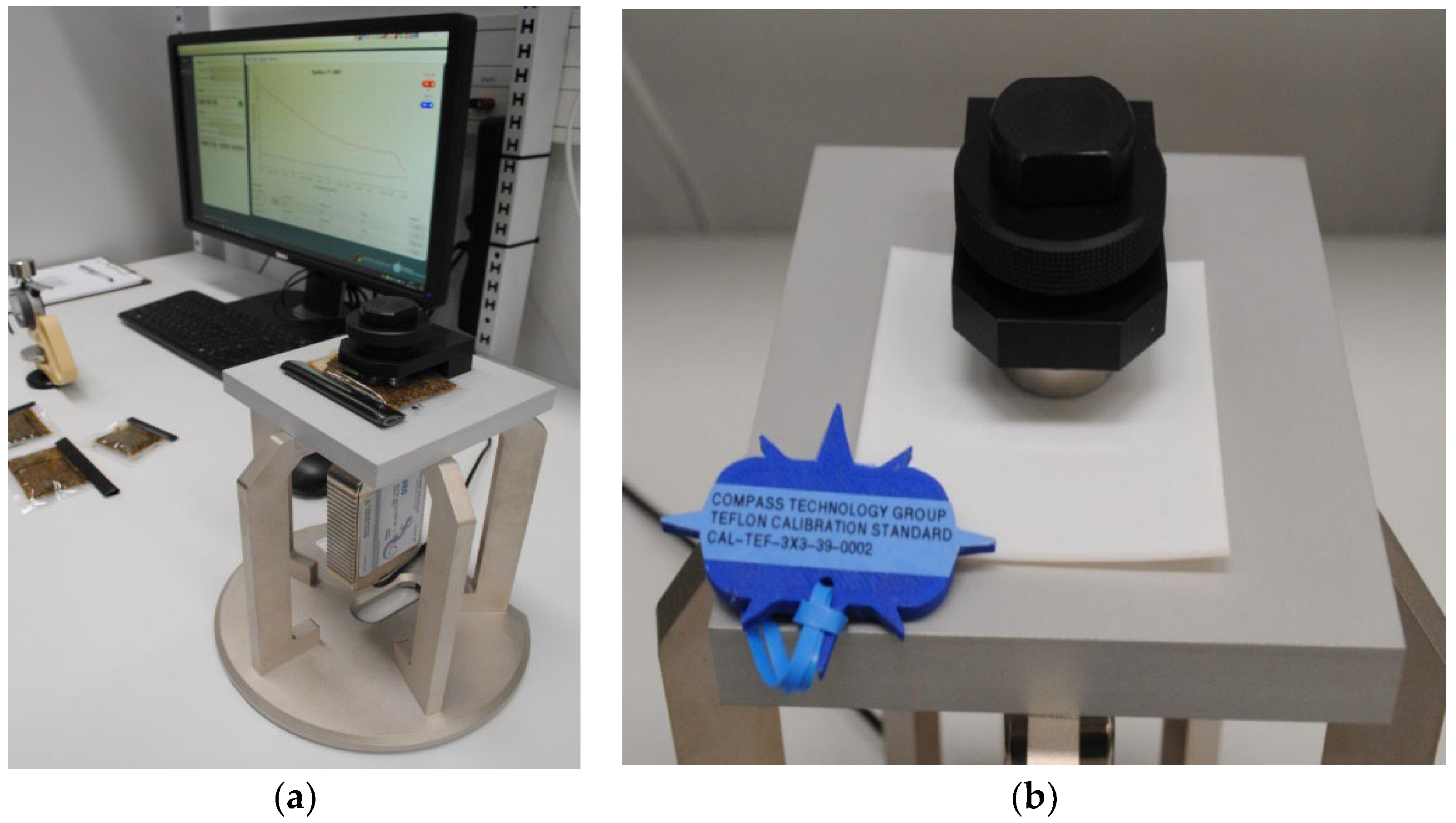
The testing of the effects of electromagnetic fields on live organisms is a complex process. The difficulty with an overall assessment of the effects lies in the ignorance of interdependences between the behaviour, physiology, and thermal phenomena. The thermal impact is a result of absorption of electromagnetic field energy by the dielectric parts of insect bodies. There is a relation between the quantity of absorbed energy and the permittivity of dielectrics. A bee is composed of about 46 diverse tissues of varied dielectric properties and water content [33]. Such a structure has the properties of a heterogeneous dielectric material. An electric field acts on each tissue in different ways. This is why the dielectric properties are sensitive to small variations in fractional component volumes, because the permittivity of water normally differs from that of other components [34]. The complexity of a dielectric structure interferes with determinations of an effective permittivity. The effective medium parameter approximations allow for computation of the physical properties of a heterogeneous sample from its constituents.

The determination of the effective permittivity is quite complicated. It requires a precise separation of the particular tissues extracted from a great numbers of bees. The procedure is labour-consuming and requires an appropriate preparation of tissues so that they preserve their dielectric properties. At the current stage of research, the dielectric parameters of bees, namely, the loss factor and loss tangent tgδ, are unknown. Preliminary studies were undertaken to establish the dielectric properties of bees in qualitative, not quantitative terms. The question one needs to answer is whether there is a frequency range for which the permittivity values show a marked deviation. These assumptions are inspired by the results of permittivity studies for the wheat weevil [31]. The loss factor was proven to reach its maximum at 39 MHz. The mortality of the wheat weevil exposed to an electric field turns out to be greater at 39 MHz than at 2.45 GHz, for which water particles are excited to intense vibrations.

This stage of research was designed to determine the value of the loss factor as an imaginary part of effective permittivity ${\epsilon }_r^{″}$ and the loss tangent tgδ for a homogenate of worker bee bodies produced by mixing dead insects at field frequencies ranging from 1 MHz to 6 GHz. The bees were killed at −18 °C, then the homogenate was made. The samples have an instable structure and flexible form. It is assumed that a band of radio frequencies exists where the loss factor ${\epsilon }_r^{″}$ becomes extreme.

Many techniques and principles of testing permittivity in biological tissues are similar to those applied to traditional engineering materials. A two-layer sample of a multiphase dielectric can be expressed in a simplified composition [35]. The Bottcher–Bordewijk model suggests a very good feasibility of predicting the permittivity of complex mixtures [36]:

$$\frac{3{\epsilon }_1}{2{\epsilon }_{eff1}+{\epsilon }_1}{\phi }_1+\frac{3{\epsilon }_2}{2{\epsilon }_{eff1}+{\epsilon }_2}{\phi }_2=1$$

(1)

where ${\epsilon }_i$ is the permittivity of pure components, ${\phi }_i$ is the volume of each component, and ${\epsilon }_{eff1}$ is the effective permittivity.

For a two-phase composition, the volume fraction is as follows:

${\phi }_2=1-{\phi }_1$ and ${\phi }_1=\phi$.

The Skipetrov model can be used to describe the constituent materials; the two-phase system equation is [37]:

$${\epsilon }_{eff2}={\epsilon }_1\left(1+\frac{3\phi \left({\epsilon }_2-{\epsilon }_1\right)}{{\epsilon }_1\left(2+\phi \right)+{\epsilon }_2\left(1-\phi \right)}\right)$$

(2)

Skipetrov explored the effective permittivity of a random medium. The particle volume fraction $\phi$ is assumed to be much smaller than unity. Another model the Maxwell-Gannet, where the two-phase multisystem of spherical particles is as follows [38]:

$${\epsilon }_{eff3}={\epsilon }_1-3\phi {\epsilon }_1\frac{{\epsilon }_1-{\epsilon }_2}{{\epsilon }_2+2{\epsilon }_1}$$

(3)

Maxwell-Gannet offered a permittivity model for complex biological tissues, which can be regarded as a small ball distributed in a continuum.

The problem of heterogeneity of a two-layer antenna medium can be reduced to a homogeneous dielectric system and effective permittivity can be expressed as follows [39]:

$${\epsilon }_{eff4}={\left({\displaystyle \sum _{n=1}^N\frac{t_n}{{\epsilon }_n}}\right)}^{-1}·{\displaystyle \sum _{n=1}^N{t}_n}$$

(4)

where ${\epsilon }_n$ is the permittivity of the nth layer, and t_n is the thickness of the nth layer.

It is additionally assumed at the present stage that the magnetic permeability of dielectric biological materials is the same as of vacuum, namely, µ = µ₀. The knowledge of electromagnetic properties of biological tissues is virtually identical with the knowledge of their electric properties.

3. Methodology

The method of testing the dielectric properties of the bee homogenate involves the selection of the measurement device, that is, an epsilometer from Compass Technology (Compass, Inc., New York, NY, USA) integrated with Copper Mountain R60 1-Port Vector Network Analyzer (Copper Mountain Technologies, Indianapolis, IN, USA). Several criteria of equipment selection were taken into account:

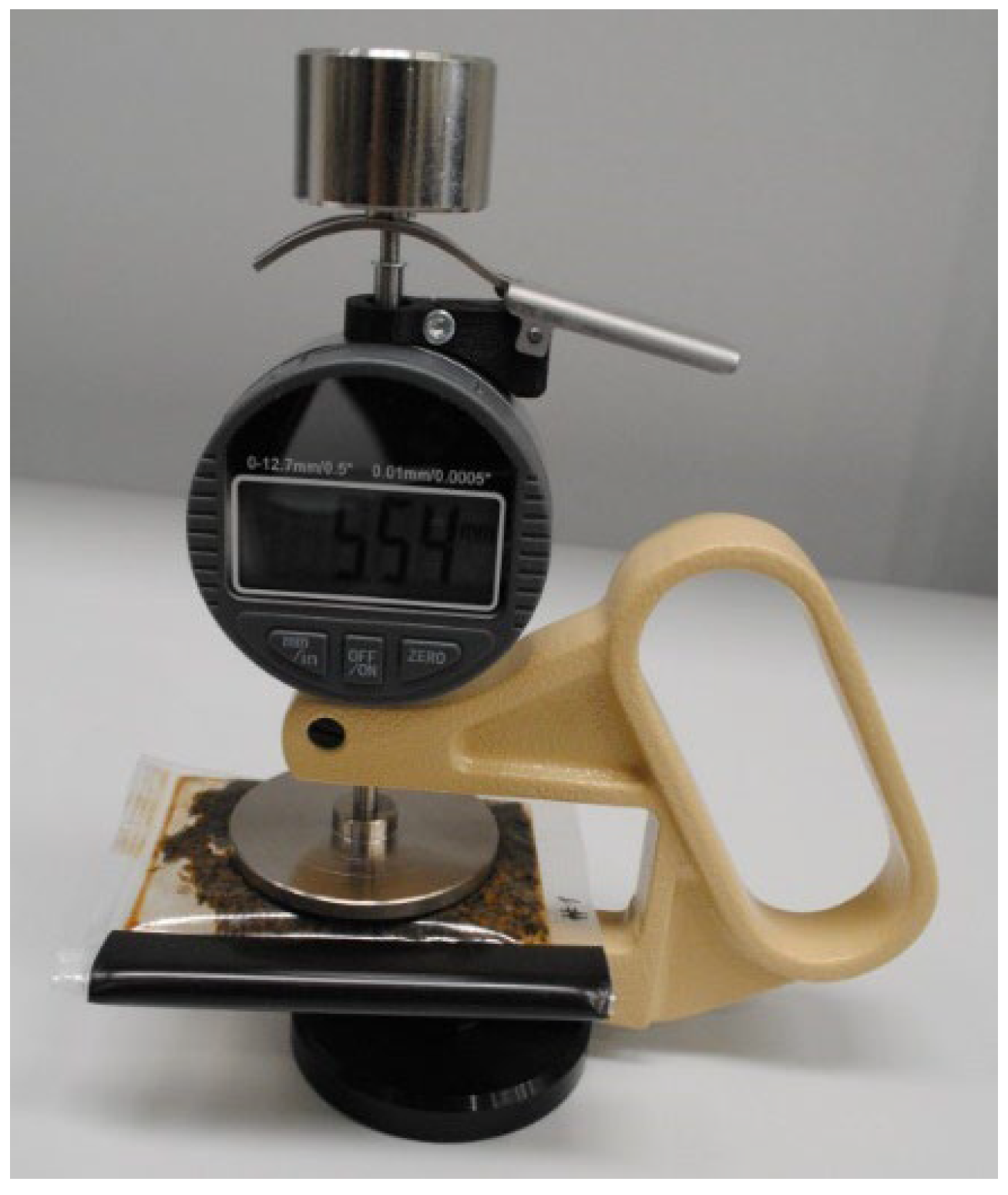
• The quantity of the test material should be minimal to avoid killing an excessive number of bees. The minimal sample thickness of 0.3 mm and the surface area of epsilometer capacitor electrodes A = 2.12 cm² meet this condition;
• The method of double-layer permittivity measurement can be applied by placing the gelatinous medium inside polyurethane sachets;
• Placing the medium in the sachets allows for the air to be sucked off in order to limit interference with the measurement results;
• The epsilometer manufacturer guarantees the accurate measurements of permittivity up to the relative value of 25 and, with a lower accuracy, up to 40;
• The possible frequency range of epsilometer testing of the material under test (MUT) is 1 MHz ÷ 6 GHz, which meets the requirements of the study.

State-of-the-art equipment featuring analytical corrections of parasitic impedances and fringing fields is used for the study of bee homogenate and its dielectric properties—Compass Technology Epsilometer with an integrated Copper Mountain R60 1-Port Vector Network Analyzer. The epsilometer is a device that measures dielectric substrate materials to determine complex permittivity from 1 MHz to up to 6 GHz. It represents a new measurement method based on the parallel plate capacitor concept. Unlike the conventional capacitive measurement devices, this new method uses a greatly simplified calibration procedure and is capable of measuring at frequencies from 1 MHz to 3 GHz, and in some cases even up to 6 GHz. It overcomes the parasitic impedance limitations in conventional capacitor methods by explicitly modelling the fixture with a full-wave computational electromagnetic code. Specifically, a finite difference time domain (FDTD) code is used to not only design the fixture, but to create a database-based inversion algorithm as well. The inversion algorithm converts measured fixture reflection (S₁₁) into dielectric properties of a material under test MUT.

An advantage of the analyser is the possibility of establishing complex permittivity and dielectric loss factor across a broad frequency band by means of a simple and non-destructive method. Material samples are placed in the meter between the capacitor electrodes and scanned to generate a microwave response as a function of frequency. The bottom electrode is connected directly to the integrated vector network analyser R60. The absence of a wire to connect both the elements enhances the accuracy of measurement. The testing is highly simple, without requiring extra reagents, the measurement process is brief.

The epsilometer is a device dedicated to measure permittivity up to 25, although the manufacturer allows for reading its values of up to 40. Given the water content, the permittivity of insect tissue may reach above 40 for frequencies over 100 MHz [40]. Some initial testing was therefore undertaken to verify whether the epsilometer can serve the testing of bee homogenate. The maximum values of the real part of complex permittivity were below 40 and did not exceed 39 across the frequency range.

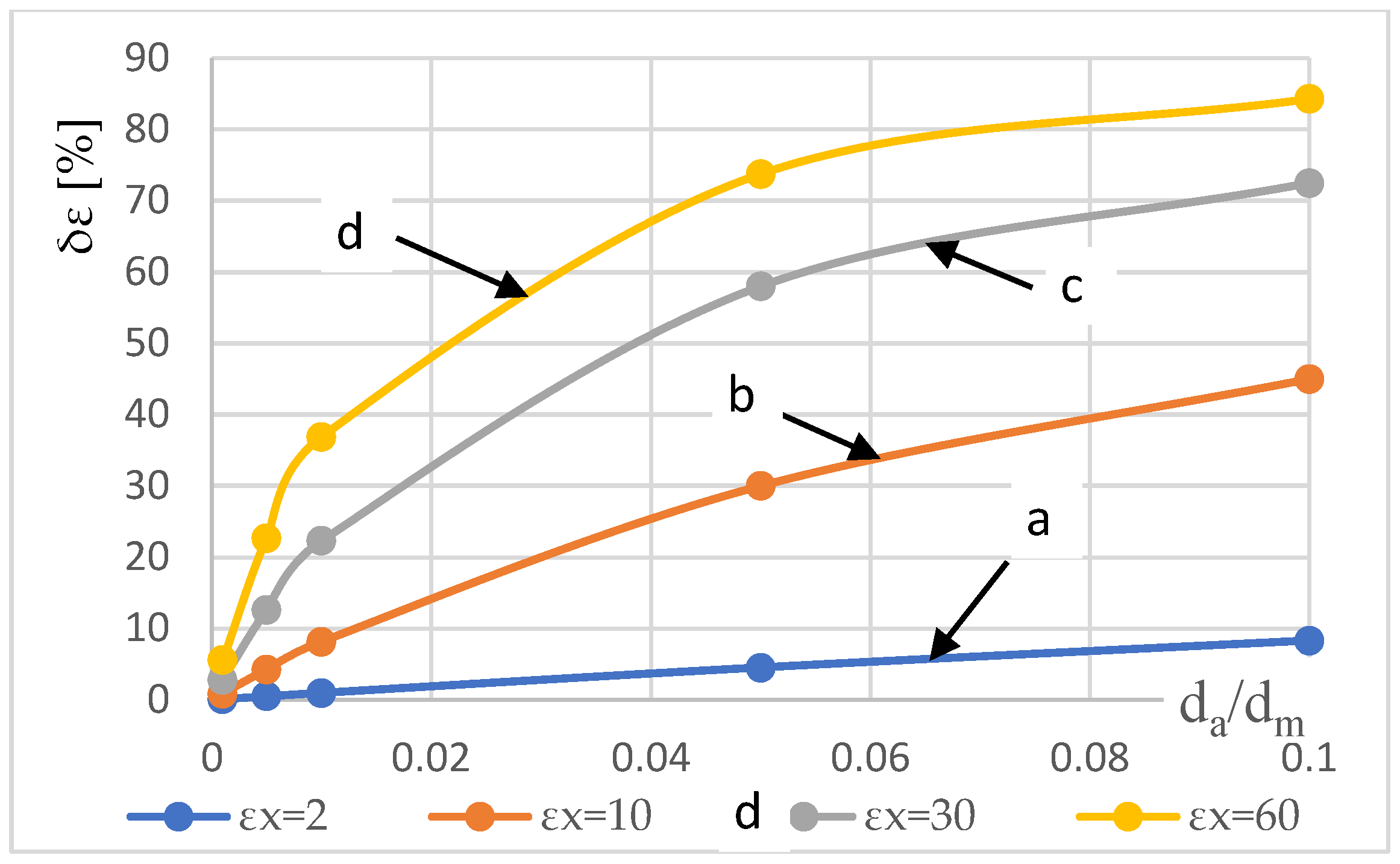
3.1. Equivalent Circuit Models of Capacitors

At the current stage of testing, the properties of effective permittivity of the bees are tested using the homogenate of mixed worker bee bodies. The physical and chemical properties may change, affecting the final results. This is particularly true for hemolymph. Promptly on mixing, the samples are placed inside polyurethan sachets to keep the water content constant. Such a sample is a kind of homogenate whose dielectric properties are close to the effective permittivity of a bee. It is one of the elements serving to determine the quantity of electric field energy absorbed by the dielectric material [31,41,42].

For dielectric materials, impedance analysis typically uses two parallel electrodes on either side of the sample, which is equivalent to a capacitor. A time-varying electric field is applied to the electrodes to interact with the material under test (MUT). The measured impedance (including resistance and capacitance) can be analytically related to dielectric permittivity with additional knowledge of the capacitor geometry. The impedance analysis method is often described as a cluster technique. Usually, the effects of parasitic impedances and edge fields are assumed to be small enough to be empirically corrected. Without parasitic effects, the dielectric permittivity ${\epsilon }^{\ast }$ is a function of the surface A of the electrodes, the distance d between them, and the measured impedance Z and can be expressed [43] as:

$$\frac{1}{Z}=G+j\omega C_p=j\omega C_o{\epsilon }^{\ast }$$

(5)

for:

${\epsilon }^{\ast }=\frac{C_p}{C_o}-j\frac{G}{\omega C_o}$—complex permittivity, where C_p is the capacitance of MUT [F], and G is the conductance of MUT, the measured value as dissipation factor.

Permittivity ${\epsilon }^{\ast }$ describes the interaction of a material with an electric field. Complex relative permittivity ${\epsilon }_r^{\ast }$ is equivalent to the complex permittivity ${\epsilon }^{\ast }$ relative to the permittivity of free space ${\epsilon }_o$:

$${\epsilon }_r^{\ast }=\frac{{\epsilon }^{\ast }}{{\epsilon }_o}={\epsilon }_r^{\prime }-j{\epsilon }_r^{″}$$

(6)

where ε₀ = 8.854 × 10⁻¹² F/m—the permittivity of free space.

The real part of the complex relative permittivity ${\epsilon }_r^{\prime }$ is a measure of how much energy from an external field is stored in a material. The imaginary part of complex relative permittivity ${\epsilon }_r^{″}$ is called the loss factor and is a measure of how dissipative or lossy a material is to an external field. The real ${\epsilon }_r^{\prime }$ and imaginary ${\epsilon }_r^{″}$ parts of permittivity are:

$${\epsilon }_r^{\prime }=\frac{d{C}_p}{A{\epsilon }_o}$$

(7)

$${\epsilon }_r^{″}=\frac{dG}{\omega A{\epsilon }_o}$$

(8)

where ${\epsilon }_r^{\prime }$ is the real part of complex relative permittivity, ${\epsilon }_r^{″}$—the imaginary part of complex relative permittivity, d is the distance between the capacitor electrodes [m], and A is the guarded electrode’s surface area [m²].

The sum vector ${\epsilon }_r^{\ast }$ represents complex permittivity and makes an angle δ with the real relative permittivity vector ${\epsilon }_r^{\prime }$. The losses in the dielectric can be described by the loss tangent $\mathrm{t}\mathrm{g}\delta$ (for $\mu ={\mu }_0$):

$$\mathrm{t}\mathrm{g}\delta =\frac{{\epsilon }_r^{″}}{{\epsilon }_r^{\prime }}$$

(9)

On the basis of (6) and (9), the following is correct:

$${\epsilon }^{\ast }={\epsilon }_0{\epsilon }_r^{\prime }\left(1-j\mathrm{tg}\delta \right)$$

(10)

Loss tangent tgδ is a determinant of loss, expressed with the energy of the electric field absorbed by the dielectric. The power absorbed by a dielectric material subjected to an electric field is given by the following relationship [31,41]:

$$P=E^2\sigma =E^2\omega {\epsilon }_r^{″}{\epsilon }_0=55.63f{E}^2{\epsilon }_r^{″}\cdot {10}^{-12} [{\mathrm{W}/\mathrm{m}}^3]$$

(11)

where P is the power density per unit volume [W/m³], E is the electric field strength [V/m], and f is the frequency [Hz].

Even with the above techniques, the capacitance method is typically limited to the frequencies below 100 MHz. The frequency range can be extended up to 1 GHz by careful electrode design. In these cases, parasitic impedance must be further minimized and accuracy at the upper frequency of the measurement range is limited. High frequency capacitance methods require a complicated calibration process that uses a series of calibration measurements for both the high frequency analyser and separately for the capacitance fixturing.

The dielectric permittivity is achieved by measuring the capacitance of the electrodes directly in contact with the MUT. When the MUT is in direct contact with the electrodes, an airgap is formed between the MUT and the electrodes. No matter how flat and parallel both sides of the MUT are, an air gap forms. This air gap is the cause of measurement error because the measured capacitance is the series connection of the capacitance of the dielectric material and the airgap. Measurement error δε is a function of the relative permittivity ${\epsilon }_r^{\ast }$ of the MUT, thickness of the MUT d_m, and the air gap thickness d_a. The relationship between the air gap thickness d_a and measurement error δε is determined by the equation:

$$\delta \epsilon =\frac{{\epsilon }_x-{\epsilon }_r^{\ast }}{{\epsilon }_x}=\frac{{\epsilon }_r^{\ast }-1}{\frac{d_m}{d_a}+{\epsilon }_r^{\ast }}$$

(12)

where $C_o={\epsilon }_o\frac{A}{d_a}$ is the capacitance of air gap, $C_x={\epsilon }_x{\epsilon }_o\frac{A}{d_m}$ is the capacitance of measured material, and $C_{err}=\frac{C_x{C}_o}{C_x+C_o}={\epsilon }_{err}{\epsilon }_o\frac{A}{d_m+d_a}$ is the measured capacitance.

Figure 1 presents the influence of the air gap thickness d_a of the tested sample on the error value $\delta \epsilon$ of the measured permittivity ${\epsilon }_x$.The effect is greater with thin materials and a high permittivity ε_x of materials. This air gap effect can be eliminated by applying thin film electrodes to the surfaces of the dielectric material.

In most cases, the edge field cannot be ignored and there are various strategies for either minimizing it or correcting for it, e.g.,:

• Designing the electrode spacing to be much smaller than the lateral dimensions reduces the importance of these edge fields;
• Fixing the guard ring into one of the electrodes;
• Analytical corrections can be applied to the data.

The Copper Mountain Epsilometer was refined by taking into account analytical corrections of the complex calibration procedures and the high frequency limitations of traditional impedance analysis techniques. It includes a fixture that resembles the geometry of a parallel-plate capacitor and has the advantages of the conventional method, including a non-destructive and simple measurement procedure. More importantly, the method enables higher frequency measurement by implementing a new inversion technique based on a full-wave, finite difference time domain (FDTD) solver. The FDTD solver is used to exactly model the measurement geometry, accounting for all edge fields as well as parasitic capacitances and inductances that plague conventional impedance analysis methods. In addition, the FDTD solver is used in a way that allows:

4.

An inversion of frequency dependent dielectric properties in seconds and;

5.

Avoiding the need to bring the full-wave computational electromagnetic CEM modelling expertise to the measurement laboratory [44].

3.2. The Preparation of the Materials under Test MUT

Five samples of biological material, placed in hermetically sealed (by sucking off the air) polyurethan sachets, were prepared for the testing of bee dielectric properties. The biological material has the properties of a quasi-homogenate. The bees were withdrawn from a family living in the upper part of a frame. The samples were prepared by killing the bees at −18 °C. A reasonable (about 100) number of bees necessary to meet the epsilometer measurement requirements was adopted. The bees originated from three different families. Prior to the measurements, they were defrosted and mixed at the room temperature to produce a homogenous structure. A weighted quantity of the material (circa 15 cm³) was then placed inside the bags, the air was sucked off, and all the edges were heat-sealed. The sample had a gelatinous (elastic) consistency and did not dry, its humidity remained constant during the measurements. The sacheted samples were numbered #1 through #5.

The dielectric properties of tissues are affected by many factors, including frequency, temperature, and moisture content. Our tests were designed for the room temperature (19 °C) only. The bee homogenate moisture content is identical in the entire sample volume. A certain moisture heterogeneity in the sample is caused by chitin, which does not absorb water. The water content in the particular tissues of a live bee highly varies. Chitin contains no water, the moisture content in body fat is around 16%, in muscular tissue it is 65%, and in hemolymph it is 90%. A greater amount of water increases permittivity [45]. For the tested homogenate samples, permittivity is below 39 all across the frequency range.

The measurement uncertainty of bee homogenate permittivity is also due to shape changes in the bee biological tissue cells caused by the pressure force of the measurement device [46,47]. The cell damage in the process of preparation for testing, crushing, and the changes in physical and chemical properties of the hemolymph of a killed bee additionally affect measurement errors. Therefore, the test results fail to reflect the permittivity of a living bee. The end results are also influenced by other objective factors such as bee species and age, environmental conditions in connection with ambient temperature and humidity, and the nature of work bees carry out in their hive. Given the complex conditions of establishing permittivity of live bees, the changes relating to this uncertainty are assumed to be acceptable for the purpose of determining the insects dielectric properties at the present stage of research.

Following the theoretical part of this paper, the sample thickness must be specified for a correct determination of the dielectric parameters of the biological bee material, that is, the bee body homogenate. Both the sachet surfaces need to be flat so that they adhere to the epsilometer capacitor electrodes without forming empty spaces (with the air alone). For instance, the measurement error is below 10% for the air gap $d_a<0.04\mathrm{mm}$ in the case of the expected ${\epsilon }_r^{″}<30$ and a sample thickness of 4 mm (Figure 1). This example nonetheless shows that testing needs to be carried out conscientiously and with particular attention.

The thickness of the samples is established with a Checkline J-40-T digital thickness gauge (Figure 2). The gauge measurement marks conform to EN ISO 5084 [48]. The device measurement range is (0–10) mm, its resolution 0.01 mm, the flat measurement foot has a diameter of 50.42 mm, and the maximum pressure is 1 kPa. The samples in question have a delicate, dissolving structure whose thickness is affected by even a minor pressure. The same force of pressure is applied to every sample in order to maintain the reproducibility of measurements. The results of thickness measurements for the individual samples of the biological materials are listed in

Table 2. Measurement results of worker bee body homogenate thickness.

Sample Number	Thickness, [mm]
1	3.7
2	3.2
3	5.5
4	4.7
5	4.5

.

The method of preparing the test samples inside the polyurethane sachets causes the measured permittivity to include two loss factor components, for the polyurethane and for the bee homogenate. The thickness of the sachet walls is d = 0.2 mm. Using (1) ÷ (4), the dependences specifying the real value for the homogenate are shown below.

The loss factor ${\epsilon }_{2\_1}$ dependence is based on (1):

$${\epsilon }_{2\_1}=2{\epsilon }_{eff1}\frac{2{\epsilon }_{eff1}+\left(1-3\phi \right){\epsilon }_1}{3\left(1-\phi \right)\left(2{\epsilon }_{eff1}+{\epsilon }_1\right)-\left(1-3\phi \right){\epsilon }_1-2{\epsilon }_{eff1}}$$

(13)

The loss factor ${\epsilon }_{2\_2}$ results from (2):

$${\epsilon }_{2\_2}=2{\epsilon }_1\frac{\left(2+\phi \right)\left({\epsilon }_{eff2}-{\epsilon }_1\right)+3\phi {\epsilon }_1}{3\phi {\epsilon }_1+\left(1-\phi \right)\left({\epsilon }_1-{\epsilon }_{eff2}\right)}$$

(14)

The loss factor ${\epsilon }_{2\_3}$ is derived from (3):

$${\epsilon }_{2\_3}={\epsilon }_1\frac{2{\epsilon }_{eff3}-\left(2-3\phi \right){\epsilon }_1}{\left(1+3\phi \right){\epsilon }_1-{\epsilon }_{eff3}}$$

(15)

The loss factor ${\epsilon }_{2\_4}$ is based on (4):

$${\epsilon }_{2\_4}=\frac{{\epsilon }_{eff4}{\epsilon }_1{t}_2}{{\epsilon }_1\left(t_1+t_2\right)-{\epsilon }_{eff4}{t}_1}$$

(16)

These calculated values of the loss factors differ from the measured values. The error inherent in the determination of the real homogenate loss factor is defined by:

$$\delta {\epsilon }_2=\left|\frac{{\epsilon }_{r\_i}^{″}-{\epsilon }_{2\_i}}{{\epsilon }_{r\_i}^{″}}\right|·100\%$$

(17)

where ${\epsilon }_{r\_i}^{″}$ is the measured value of the loss factor for ith sample, $i=1\dots 5$; and ${\epsilon }_{2\_i}^{″}$—the calculated value (13) ÷ (16) of the loss factor for ith sample, $i=1\dots 5$.

3.3. The Analysis of Measurement Results

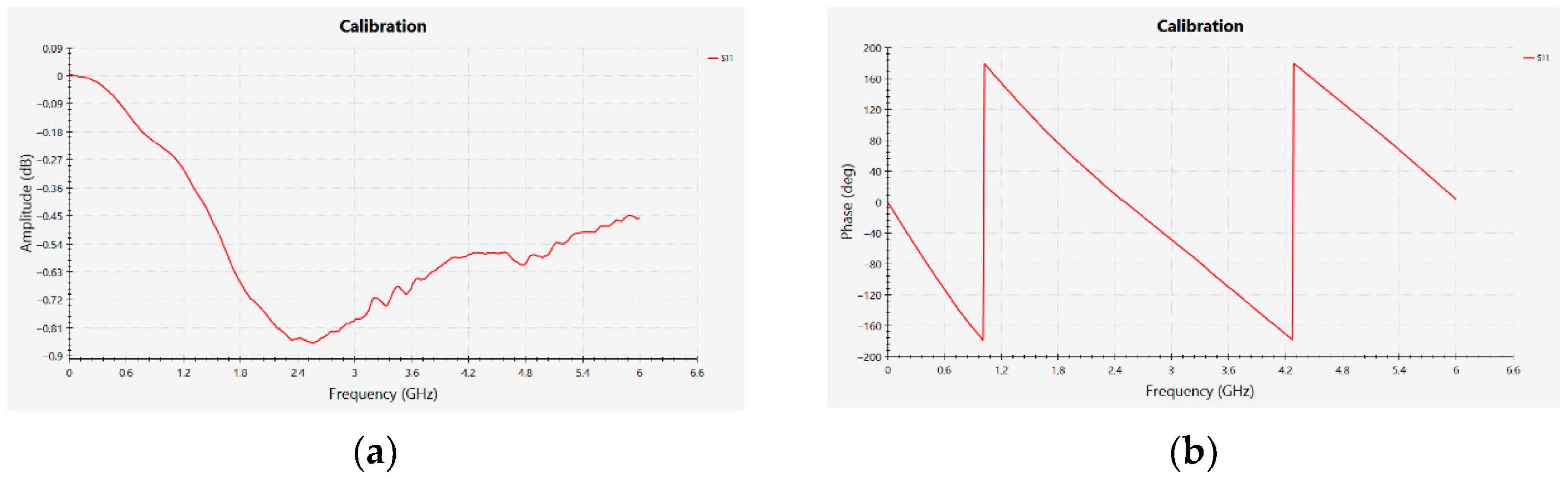
3.3.1. Stand Calibration

Determining the imaginary part of complex relative permittivity (loss factor) ${\epsilon }_r^{″}$ and loss tangent tgδ of the bee homogenate material samples is the final part of experimental testing. The measurements use the epsilometer system consisting of the Compass Technology measurement device, the Copper Mountain R60 Vector Network Analyzer (VNA), and a software package dedicated to the establishment of dielectric material parameters within the band 1 MHz to 6 GHz (Figure 3b) [49].

The measurement process begins with calibrating the stand (Figure 3b) by means of a dedicated Teflon calibrator (Compass Technology, Teflon Calibration Standard, CAL-TEF-3X3-39-002). The process generates the amplitude and phase curves which become the points of reference for the Compass Technology measurement device (Figure 4a,b).

3.3.2. Measurement Results

Results for the thickness of individual samples (Table 2) are the starting point for a determination of the parameters of complex permittivity. The measurement results for the particular samples #1 ÷ #5 are shown in Figure 5, Figure 6 and Figure 7. The graphs including the designations ${\epsilon }_r^{″}\_1÷5$ present the loss factor. The figures including the designations tgδ_1 ÷ 5 show the loss tangent tgδ. The measurement results serve the calculation of power density P per unit volume (11), which determines the quantity of absorbed power. The results of these calculations are depicted in the Figures designated ‘P_1 ÷ 5’. The numbering 1 to 5 denotes the number of a test sample.

All the characteristics of the test samples properties are shown as logarithmic curves. For the purpose of a more detailed interpretation of the samples’ dielectric properties, the parameters are presented for two frequency ranges: 1 MHz–6 GHz (Figure 5a, Figure 6a and Figure 7a) and 1 MHz–1 GHz (Figure 5b, Figure 6b and Figure 7b). The results suggest the loss factor ${\epsilon }_r^{″}$ has two extremes (Figure 5). The first maximum is in the frequency range of 20 MHz–60 MHz. The loss factor ${\epsilon }_r^{″}$ varies for the individual samples and is within the 10.5 ÷ 18.5 range. This denotes a measurement error of approximately 40%. One can assume the error is a consequence of an inadequate preparation of samples due to the air presence in the sachets. With reference to Figure 1, depicting the impact of air gap on permittivity measurements, the ratio of the air gap thickness to the thickness of the MUT tested material, for loss factor ${\epsilon }_x\approx 20$, can be assumed to be around $\raisebox{1ex}{$d_a$}\!\left/ \!\raisebox{-1ex}{$d_m$}\right.=0.03$. This means the width of the air gap reached $d_a\approx 0.1 \mathrm{mm}$.

The losses are expressed as the loss tangent tgδ (Figure 6). The results prove that tgδ also becomes extreme at the frequencies close to those of imaginary part of permittivity ${\epsilon }_r^{″}$ extremes and is in the 20 ÷ 80 MHz range. tgδ varies in the 0.3 ÷ 0.46 range. These values show a tendency of power absorbed variations, yet without representing their values.

Power density per volume unit P [kW/m³] (11) is determined to this end (Figure 7). The results fail to show a significant impact of the loss factor ${\epsilon }_r^{″}$ on the power density P. This means the quantity of absorbed electric field energy, and thus the temperature increment, are more dependent on the frequency.

The Compass Technology Epsilometer can test samples up to 6 GHz. The effects of the electric field frequency on permittivity properties of the bee homogenate were tested in the same frequency range. Substantial result discrepancies are generated for frequencies above 3 GHz, in particular with regard to the samples #1 and #5. The results above 3 GHz were not analysed; therefore, the probable uncertainty of measurements in that range is reported in [44].

3.3.3. The Calculation of Homogenate Dielectric Properties

The homogenate samples for the testing of dielectric properties generate results in the form of effective permittivity. In order to compute the loss factor for the homogenate only, Equations (13)–(16) were used. The initial analysis results are part of

Table 3. The initial results of permittivity calculations.

	Sample Number
	#1	#2	#3	#4	#5
${\epsilon }_r^{″}$	13	10.5	18.5	12	15
${\epsilon }_{2.1}$	13.78	11.17	19.32	12.54	15.77
${\epsilon }_{2.2}$	−7.03	−7.43	−6.54	−6.83	−6.75
${\epsilon }_{2.3}$	−6.46	−6.73	−6.19	−6.4	−6.31
${\epsilon }_{2.4}$	16.06	12.06	22.98	13.85	18.43
	[%]	[%]	[%]	[%]	[%]
$\delta {\epsilon }_{2.1}$	6.03	6.38	4.45	4.51	5.16
$\delta {\epsilon }_{2.2}$	154	170	135	156	145
$\delta {\epsilon }_{2.3}$	149	164	133	153	142
$\delta {\epsilon }_{2.4}$	23.52	20	24.21	15.38	22.86

. For the samples #1÷#5 and the maximum imaginary part of permittivity, the loss factor ${\epsilon }_{2.i}^{″}$ is calculated (for i = 1 ÷ 5) and the measurement error δε_2.i is determined (for i = 1 ÷ 5) in line with (17). Preliminary calculations showed ${\epsilon }_{2.2}^{″}$ and ${\epsilon }_{2.3}^{″}$ produce wrong results beyond the domain of permittivity values. They are of no use to the continuing analysis.

The values of bee homogenate loss factor ${\epsilon }_{2.1}^{″}$ calculated as per (13) are illustrated in Figure 8a. The error δε_2.1 shown with the differences between the measured and calculated values is presented in Figure 8b. The parallel changes in the loss factor ${\epsilon }_{2.2}^{″}$ and the error δε_2.2 are depicted in Figure 9. A comparison of the changes shown in Figure 8a and Figure 9a points to the substantially greater values of the loss factor determined by the method expressed by (16). The errors are considerable as well, in excess of 10% in the frequency range 10 MHz ÷ 100 MHz. The calculation error according to the method expressed by (13) is below 7% across the frequency range.

The foregoing analysis implies that the method of calculating the loss factor developed by Bottcher–Bordewijk (13) is useful to the test method adopted in this paper. This conclusion seems disputable since (16) is based on the assumption that the two sample components form the parallel planes of the antenna structures with n layers. Equation (13) assumes a cell structure of a random nature with some predictable average properties such as cell size and density. It can be modelled with randomly distributed spherical shells. This is a generalised model of a dielectric material. This implies that a spherical approach to the proposed model of calculations is more reasonable. It is supported by the cellular properties of the homogenate, other than those characteristic for the antenna structures. The correct results of Bottcher–Bordewijk method (13) also relate to the volume fraction of polyurethane, which fulfils the condition and is in the range: $\phi \in \left(0.04÷0.06\right)$.

3.4. A statistical Review of the Results

A statistical analysis is applied to the results for loss factor ${\epsilon }_r^{″}$ and loss tangent tgδ and Pearson’s coefficient is determined for the samples of bee origin biological materials in the limited frequency band 1 MHz–3 GHz (

Table 4. Pearson’s coefficient for ${\epsilon }_r^{″}$ measurements in the 1 MHz to 3 GHz band.

Sample Number	${\mathit{\epsilon }}_{\mathit{r}}^{″}$
	#1	#2	#3	#4	#5
#1	1	0.993	0.968	0.999	0.990
#2	0.993	1	0.940	0.988	0.970
#3	0.968	0.940	1	0.976	0.991
#4	0.999	0.988	0.976	1	0.994
#5	0.990	0.970	0.991	0.994	1

and

Table 5. Pearson’s coefficient for tgδ in the 1 MHz to 3 GHz band.

Sample Number	tgδ
	#1	#2	#3	#4	#5
#1	1	0.989	0.987	0.971	0.962
#2	0.989	1	0.983	0.990	0.983
#3	0.987	0.983	1	0.954	0.993
#4	0.971	0.990	0.954	1	0.993
#5	0.962	0.983	0.947	0.993	1

).

The variations in ${\epsilon }_r^{″}$ and tgδ across the samples are caused by the difficulties of determining the sample thickness. The biological material homogenate in the sachets exhibits gelatinous properties and is of an elastic structure. As the samples are inserted between the capacitor electrodes, it is technically impossible to control the pressure force of the head of the Compass Technology measurement device. The force should correspond to that in the Checkline J-40-T digital thickness gauge that measures a sample thickness and be specified to the level of 1 kPa. Nonetheless, within the defined frequency band the statistical analysis results are strongly correlated among the samples of honeybee worker homogenate (Table 4 and Table 5). This allows for the acceptance of the uncertainty arising from the method of determining the parameters of the media materials.

3.5. Measurement Uncertainties

Measurement uncertainty for the epsilometer may arise from a number of error sources. Systematic errors can be caused by computational modelling errors, fixture manufacturing variations, and VNA nonlinearities. The calibration procedure with a known material is designed to minimize these systematic errors (Figure 3b). The estimated uncertainty of imaginary permittivity for the 2.3 mm Teflon was applied. In addition, VNA drift and noise, electrode pressure variation, and sample thickness uncertainty can influence measurement uncertainty. In this case, the variation is generally less than 2% starting from 10 MHz. For other cases, the measurement uncertainty may vary from 0.5% to 5% depending on thickness and permittivity [50].

The above uncertainty example does not account for the thickness error (Figure 1). There may be an additional uncertainty component proportional to the MUT thickness accuracy. A micrometre rather than callipers should be used to measure thickness to minimize this uncertainty [44]. The digital thickness gauge Checkline J-40-T is used to measure the thickness of the honeybee worker homogenate.

Another significant uncertainty can occur with homogeneous samples of gelatinous (elastic) properties that are not exactly flat. The material subject to MUT testing is placed in a polyurethan sachet in order to suck out the air and then seal the edges. In this scenario, the sample humidity remains steady and the MUT can be positioned between the electrodes. Any air gap between the MUT and the electrodes results in a significant measurement error. The error is especially pronounced at higher permittivity (Figure 1). The test samples are expected to suffer from an additional, systematic error associated with the sachet material, different to that of the bee homogenate. The material has a certain thickness too, which affects the final measurement result.

4. Discussion

The dielectric properties of a honeybee worker homogenate packaged into polyurethan sachets were analysed in this paper. The variations in the loss factor ${\epsilon }_r^{″}$, the loss tangent tgδ, and the power density per unit volume P as a function of the frequency in the range 1 MHz to 6 GHz were studied. The results in a graphic form determined two areas of extreme values of the loss factor and loss tangent tgδ: the first for frequencies around 20 ÷ 60 MHz and the other, above 3 GHz. Due to high uncertainty of measurements above 3 GHz, these results were ignored in the discussion. The obtained variations in the dielectric properties of the bee homogenate fill the literature gap. The extremes of the two dielectric variables point to a frequency area of a more intense impact of the electric field. The calculated power density per unit volume P fails to display any particular variations such as extremes in this area. Such an interpretation would indicate a more intense growth of the absorbed energy with rising. This would mean the absorbed energy would produce greater temperature increments for frequencies outside the area of the extreme imaginary part of permittivity. A temperature rise above 50 °C may result in death of the insects [51].

A methodology of measuring the dielectric properties of the bee homogenate is an important result of this study. It helps to reduce the killing of bees to a minimum. The gelatinous sample in the sachets, from which the air was sucked out, preserves its homogenous structure. The sample is subject to simple measurement procedures in the epsilometer from Compass Technology, integrated with a Copper Mountain R60 1-port Vector Network Analyzer. The measurement technique assures an accurate reading of the loss factor and loss tangent tgδ within the frequency range of 1MHz ÷ 3GHz. The thin wall of the polyurethane sachet interferes with the measurement. Based on the method of determining effective permittivity developed by Bottcher–Bordewijk, a correction was introduced to eliminate the impact of the polyurethane permittivity. The method of correcting for the permittivity relies on the assumption of a spherical cell structure, which is the case of the test homogenate.

These conclusions apply to a bee homogenate which is pure matter. Beside purely electro-thermal phenomena in nature, bee behaviour and physiology that may modify the final effect of the electric field are important as well. The honeybee, as a social insect, has developed a range of specific behaviours, including those responsible for maintaining the constant temperature of the brood chamber. The results for the impact of electric field on the other insect as rice weevil can serve as an example [30,31]. Contrary to expectations, the rice weevil has been shown to die faster at the field frequency of 39 MHz than at 2.45 GHz. For the weevil, the loss factor is extreme near the frequencies of 39 MHz. It should be concluded that the test results of the bee homogenate are reliable and close to those reported in [30,31]. The results seem to imply preliminarily the bee mortality rate may even be greater for frequencies in the range 20 ÷ 60 MHz than for higher frequencies and greater values of absorbed energy.

The research should continue to verify the results for frequencies above 3 GHz. The impact of temperature and humidity on the results of sample testing in the full frequency area is unknown. The dielectric values for the bee body homogenate should be verified by examining live bees, whose structure is heterogeneous; in addition, they may respond to experimental conditions by changing their behaviour and the intensity of their physiological processes.

A precise understanding of relationships between dielectric, behavioural, and physiological properties should, in the future, help to assess the threat to the species, and its development or adaptation to the existing environmental conditions of the so-called electromagnetic smog. Conclusions will be of particular importance to assessing the response of bee families to radio frequency (RF) magnetic fields. Further studies will need to assess the field effect on bee behaviour: disorientation, over-excitation, etc. Defining a correlation between permittivity, the absorbed power, and the impact of insect temperature growth on their mortality will be important too.

5. Conclusions

Testing the dielectric properties of a bee homogenate with the Copper Mountain Technologies epsilometer is a cognitive nature and allows to fill the gaps in the literature. The loss factor and the loss tangent tgδ show a tendency similar to that shown by the results of studies of analogous parameters in the case of tissues of other insects. This confirms the correctness of the adopted research method. In the frequency range 20 ÷ 60 MHz, the loss factor and the loss tangent tgδ become extreme. The obtained results were presented using the four techniques of testing permittivity in biological tissues. The Skipetrov and Maxwell-Gannet methods of determining effective permittivity were not used in the conducted research. The smallest error in computing the honeybee homogenate permittivity was for the Bottcher–Bordewijk method. Further studies of the dielectric properties of bees should be continued, taking into account the influence of temperature, electric field strength, exposure time, and frequency on the obtained results.

References

1. Chaudhory, S.; Kumar, P.; Chaudhory, S.; Kumar, S. Hazardous Radiations from Mobile Phones and Cell Towers—A Review. JUSPS—B 2017, 29, 185–193. [Google Scholar] [CrossRef] [Green Version]
2. Balmori, A. Electrosmog and species conservation. Sci. Total Environ. 2014, 496, 314–316. [Google Scholar] [CrossRef]
3. Balmori, A. Electromagnetic radiation as an emerging driver factor for the decline of insects. Sci. Total. Environ. 2021, 767, 144913. [Google Scholar] [CrossRef]
4. Vanbergen, A.J.; Potts, S.G.; Vian, A.; Malkemper, E.P.; Young, J.; Tscheulin, T. Risk to pollinators from anthropogenic electro-magnetic radiation (EMR): Evidence and knowledge gaps. Sci. Total Environ. 2019, 695, 133833. [Google Scholar] [CrossRef]
5. Velthuis, H.H.W.; Van Dorn, A. A century of advances in bumblebee domestication and the economic and environmental aspects of its commercialization for pollination. Apidologie 2006, 37, 421–451. [Google Scholar] [CrossRef] [Green Version]
6. Polls, S.G.; Roberts, S.P.M.; Dean, R.; Marris, G.; Brown, M.A.; Jone, R.; Neuman, P.; Settale, J. Declines of managed honey bees and beekeepers in Europe. J. Apicul. Res. 2010, 49, 15–22. [Google Scholar]
7. Lázaro, A.; Chroni, A.; Tscheulin, T.; Devalez, J.; Matsoukas, C.; Petanidou, T. Electromagnetic radiation of mobile telecommunication antennas affects the abundance and composition of wild pollinators. J. Insect Conserv. 2016, 20, 315–324. [Google Scholar] [CrossRef]
8. Migał, P.; Murawska, A.; Strachecka, A.; Bieńkowski, P.; Roman, A. Changes in the honeybee Antioxidant System after 12 h of Exposure to Electromagnetic Field Frequency of 50 Hz and Variable Intensity. J. Insects 2020, 11, 713. [Google Scholar] [CrossRef] [PubMed]
9. Migał, P.; Murawska, A.; Strachecka, A.; Bieńkowski, P.; Roman, A. Honey Bee Proteolytic System and Behavior Parameters under the Influence of an Electric Field at 50Hz and Variable Intensities for a Long Exposure Time. Animals 2021, 11, 863. [Google Scholar] [CrossRef] [PubMed]
10. Migał, P.; Roman, A.; Strachecka, A.; Murawska, A.; Bieńkowski, P. Changes of selected biochemical parameters of the honeybee under the influence at an electric field at 50 Hz and variable intensities. Apidologie 2020, 51, 956–967. [Google Scholar] [CrossRef]
11. Migał, P.; Murawska, A.; Bieńkowski, P.; Strachecka, A.; Roman, A. Effect of the electric field at 50Hz and variable intensities on biochemical markers in the honey bee’shemolymos. PLoS ONE 2021, 16, e0252858. [Google Scholar] [CrossRef]
12. Shepherd, S.; Lima, M.A.P.; Oliveira, E.E.; Sharkh, S.M.; Jackson, C.W.; Newland, P.L. Extremely Low Frequency Electromagnetic Fields impair the Cognitive and Motor Abilities of Honey Bees. Sci. Rep. 2018, 8, 7932. [Google Scholar] [CrossRef] [PubMed]
13. Shepherd, S.; Hollands, G.; Godley, V.C.; Sharkh, S.M.; Jackson, C.W.; Newland, P.L. Increased aggression and reduced aversive learning in honey bees exposed to extremely low frequency electromagnetic fields. PLoS ONE 2019, 14, e0223614. [Google Scholar] [CrossRef] [PubMed] [Green Version]
14. Wyszkowska, J.; Grodnicki, P.; Szczygiel, M. Electromagnetic Fields and Colony Collapse Disorder of the Honeybee. Electr. Eng. 2019, 95, 137–140. [Google Scholar] [CrossRef] [Green Version]
15. Migdał, P.; Murawska, A.; Bieńkowski, P.; Berbeć, E.; Roman, A. Changes in Honeybee Behavior Parameters under the Influence of the E-Field at 50 Hz and Variable Intensity. Animals 2021, 11, 247. [Google Scholar] [CrossRef]
16. Erdogan, Y.; Cengiz, M.M. Effect of electromagnetic field (EMF) and electric field (EF) on some behaviour of honey bee (Apis mellifera L.). In Proceedings of the 3rd International Conference on Advanced Engineering Technologies, Bayburt, Turkey, 19–21 September 2019. [Google Scholar]
17. Harst, W.; Kuhn, J.; Stever, H. Can Electromagnetic Exposure Cause a Change in Behaviour? Studying Possible Non-Thermal Influences on Homey Bees—An Approach within the Framework of Educational Informatics. Acta Syst. 2006, 6, 1–6. [Google Scholar]
18. Darney, K.; Giraudin, A.; Joseph, R.; Abadie, P.; Aupinel, P.; Decourtye, A.; Le Bourg, E.; Gauthier, M. Effect of high-frequency radiations on survival of the honeybee (Apis mellifera L.). Apidologie 2016, 47, 703–710. [Google Scholar] [CrossRef] [Green Version]
19. Sharma, V.P.; Kumar, N.P. Changes in honeybee behaviour and biology under the influence of cellphone radiations. Curr. Sci. 2010, 98, 1376–1378. [Google Scholar]
20. Favre, D. Mobile phone-induced honeybee worker piping. Apidologie 2011, 42, 270–279. [Google Scholar] [CrossRef] [Green Version]
21. Taye, R.R.; Deka, M.K.; Rahman, A.; Bathari, M. Effect of electromagnetic radiation of cellphone tower on foraging behaviour of Asiatic honeybee. J. Entomol. Zool. Stud. 2017, 5, 1527–1529. [Google Scholar]
22. Pramod, M.; Yogesh, K. Effect of electromagnetic radiations on brooding, honey production and foraging behavior of European honeybees (Apis mellifera L.). Afr. J. Agric. Res. 2014, 9, 1078–1085. [Google Scholar] [CrossRef] [Green Version]
23. Vilic, M.; Zaja, I.Z.; Tkalec, M.; Stambuk, A.; Srut, M.; Klobucar, G.; Malaric, K.; Tucak, P.; Pasic, S.; Gaiger, I.T. Effects of a radio frequency electromagnetic field on honey beelarvae (Apis mellifera L.) differ in relation to the experimental study design. Vet. Arh. 2021, 91, 427–435. [Google Scholar] [CrossRef]
24. Colombi, D.; Thors, B.; Tornevik, C. Implication of emf exposure limits on output power level for 5G devices above 6 GHz. IEEE Antennas Wirel. Propag. Lett. 2015, 14, 1247–1249. [Google Scholar] [CrossRef]
25. Pi, A.; Khan, F. An Introduction to Millimeter-Wave Mobile Broadband Systems. IEEE Commun. Mag. 2011, 49, 101–107. [Google Scholar] [CrossRef]
26. Thielens, A.; Bell, D.; Mortimore, D.B.; Greco, M.; Martens, L.; Joseph, W. Exposure of Insects to Radio-Frequency Electromagnetic Fields from 2 to 120 GHz. Sci. Rep. 2018, 8, 3924. [Google Scholar] [CrossRef] [PubMed]
27. Toribio, D.; Joseph, W.; Thielens, A. Near Field Radio Frequency Electromagnetic Field Exposure of a Western Honey Bee. IEEE Trans. Antennas Propag. 2022, 70, 1320–1327. [Google Scholar] [CrossRef]
28. Thielens, A.; Greco, M.K.; Verloock, L.; Martens, L.; Joseph, W. Radio-Frequency Electromagnetic Field Exposure of Western Honey Bees. Sci. Rep. 2020, 10, 461. [Google Scholar] [CrossRef] [PubMed] [Green Version]
29. Thielens, A. Environmental Impact of 5G, a Literature Review of Effects of Radio-Frequency Electromagnetic Field Exposure of Non-Human Vertebrates, Invertebrates and Plants; European Parliamentary Research Service: Brussels, Belgium, 2021. [Google Scholar]
30. Nelson, S.O. Dielectric Properties of Agricultural Products—Measurements and Applications. IEEE Trans. Dielectr. Electr. Insul. 1991, 26, 845–869. [Google Scholar] [CrossRef]
31. Nelson, S.O.; Stetson, L.E. Comparative Effectiveness of 39- and 2450-MHz Electric Fields for Control of Rice Weevils in Wheat. J. Econ. Entomol. 1974, 67, 592–595. [Google Scholar] [CrossRef]
32. Yanagawa, A.; Kajiwara, A.; Nokajima, H.; Desmond-LeQuemener, E.; Steyer, J.P.; Lewis, V.; Mitami, T. Physical assessments of termites under 2.45 GHz microwave irradiation. Sci. Rep. 2020, 10, 5197. [Google Scholar] [CrossRef] [Green Version]
33. Snodrass, R.E. The Anatomy of the Honey Bee; U.S. Department of Agriculture: Washington, DC, USA, 1910.
34. Sihovola, A.H.; Kong, J.A. Effective Permittivity of Dielectric Mixtures. IEEE Trans. Geosci. Remote Sens. 1988, 26, 420–429. [Google Scholar] [CrossRef]
35. Gun, L.; Ning, D.; Liang, Z. Effective Permittivity of Biological Tissue: Comparison of Theoretical Model and Experiment. Math. Probl. Eng. 2017, 2017, 7249672. [Google Scholar] [CrossRef] [Green Version]
36. Tjia, T.H.; Bordewijk, P.; Bottcher, C.J.F. On the notion of dielectric friction in the theory of dielectric relaxation. Adv. Mol. Relax. Int. Process. 1974, 6, 19–28. [Google Scholar] [CrossRef]
37. Skipetrov, S.E. Effective dielectric function of a random medicum. Phys. Rev. B Condens. Matter 1999, 60, 12705–12709. [Google Scholar] [CrossRef]
38. Markel, V.A. Introduction to the Maxwell Garnett approximation: Tutorial. J. Opt. Soc. Am. A 2016, 33, 1244–1256. [Google Scholar] [CrossRef] [Green Version]
39. Ali, W.K.W.; Al-Charchafchi, S.H. Using equivalent dielectric constant to simplify the analysis of patch microstrip antenna with multi-layer substrates. In Proceedings of the IEEE International Symposium of Antennas and Propagation Society, Atlanta, GA, USA, 21–26 June 1998. [Google Scholar]
40. Nelson, S.O. Radio-Frequency and Microwave Dielectric Properties of Insects. J. Microw. Power Electromagn. Energy 2001, 36, 47–56. [Google Scholar] [CrossRef]
41. Nelson, S.O.; Charity, L.F. Frequency Dependence of Energy Absorption by Insects and Grain in Electric Field. Trans. ASAE 1972, 15, 1099–1102. [Google Scholar]
42. Nelson, S.O. Agricultural Applications Of Dielectric Measurements. IEEE Trans. Dielectr. Electr. Insul. 2006, 13, 688–702. [Google Scholar] [CrossRef]
43. Warnke, U. Bees, Birds and Mankind: Destroying Nature by “Electrosmog”; A Brochure series by the Competence Initiative for the Protection of Humanity, Environment and Democracy; Kentum Translators: Kempten, Germany, 2009. [Google Scholar]
44. Schultz, J.W. A New Dielectric Analyzer for Rapid Measurement of Microwave Substrates up to 6 GHz. In Proceedings of the Antenna Measurement Techniques Association Symposium (AMTA) Proceedings, Williamsburg, VA, USA, 4–9 November 2018; pp. 1–6. [Google Scholar]
45. Ondracek, J.; Brunnhofer, V. Dielectric properties of insect tissues. Gen. Physiol. Biophys. 1984, 3, 251–257. [Google Scholar]
46. Huclova, S.; Erni, D.; Fröhlich, J. Modelling effective dielectric properties of materials containing diverse types of biological cells. J. Phys. D Appl. Phys. 2010, 43, 365405. [Google Scholar] [CrossRef]
47. Vlahovska, P.M.; Gracia, R.S.; Aranda-Espinoza, S.; Dimova, R. Electrohydrodynamic model of vesicle deformation in alternating electric fields. Biophys. J. 2009, 96, 4789–4803. [Google Scholar] [CrossRef] [PubMed] [Green Version]
48. PN-EN ISO 5084; Textiles. Determination of the Thickness of Textiles. International Organization for Standardization: Geneva, Switzerland, 1999.
49. Compass Technology: Epsilometer Measurement System, User and Software Guide, November 2018. Available online: https://www.clarke.com.au/pdf/CMT_Epsilometer_User_Guide.pdf (accessed on 16 May 2022).
50. Compass Technology, Epsilometer Uncertainties, Manuals. Available online: https://coppermountaintech.com/download-files/ (accessed on 6 December 2022).
51. Kovac, H.; Käfer, H.; Stabentheiner, A.; Costa, C. Metabolism and upper thermal limits of Apis mellifera carnica and A. m. ligustica. Apidologie 2014, 45, 664–677. [Google Scholar] [CrossRef] [PubMed]
Figure 1. Measurement error δ ε as a relationship of d a d m for MUT permittivity: (a) ε x = 2 , (b) ε x = 10 , (c) ε x = 30 , (d) ε x = 60 .
Energies 15 09342 g001
Figure 2. Checkline J-40-T digital gauge measuring the thickness of bee origin biological material samples.
Energies 15 09342 g002
Figure 3. Permittivity measurement stand: (a) the set of equipment for the determination of dielectric parameters of bee homogenate samples, (b) the calibration set for the measurement stand.
Energies 15 09342 g003
Figure 4. The calibration results of the measurement system: (a) amplitude curve, (b) phase curve of the Compass Technology measurement device.
Energies 15 09342 g004
Figure 5. The imaginary part ε r of permittivity for samples #1 ÷ #5 and the following ranges of f: (a) 1 MHz ÷ 6 GHz, (b) 1 MHz ÷ 1 GHz.
Energies 15 09342 g005
Figure 6. Dissipation factor tgδ for samples #1 ÷ #5 and the following ranges of f: (a) 1 MHz ÷ 6 GHz, (b) 1 MHz ÷ 1 GHz.
Energies 15 09342 g006
Figure 7. Power density per unit volume P [KW/m3] for samples #1 ÷ #5 and the following ranges of f: (a) 1 MHz ÷ 6 GHz, (b) 1 MHz ÷ 1 GHz.
Energies 15 09342 g007
Figure 8. (a) The loss factor ε 2.1 calculated as per (13); (b) the error of δε2.1 calculations for the loss factor ε 2.1 .
Energies 15 09342 g008
Figure 9. (a) The loss factor ε 2.4 calculated from Equation (16), (b) the error of δε2.4 calculations for the loss factor ε 2.4 .
Energies 15 09342 g009