Financial Hazard Prediction Due to Power Outages Associated with Severe Weather-Related Natural Disaster Categories

Abstract

Severe weather conditions not only damage electric power infrastructure, and energy systems, but also affect millions of users, including residential, commercial or industrial consumers. Moreover, power outages due to weather-related natural disasters have been causing financial losses worth billions of US dollars. In this paper, we analyze the impact of power outages on the revenue of electric power suppliers, particularly due to the top five weather-related natural disasters. For this purpose, reliable and publicly available power outage events data are considered. The data provide the time of the outage event, the geographic region, electricity consumption and tariffs, social and economic indicators, climatological annotation, consumer category distribution, population and land area, and so forth. An exploratory analysis is carried out to reveal the impact of weather-related disasters and the associated electric power revenue risk. The top five catastrophic weather-related natural disaster categories are investigated individually to predict the related revenue loss. The most influencing parameters contributing to efficient prediction are identified and their partial dependence on revenue loss is illustrated. It was found that the electric power revenue associated with weather-related natural disasters is a function of several parameters, including outage duration, number of customers, tariffs and economic indicators. The findings of this research will help electric power suppliers estimate revenue risk, as well as authorities to make risk-informed decisions regarding the energy infrastructure and systems planning.

1. Introduction

Electric power infrastructure plays an important role for the development of any geographical area in the world. Many systems, such as water, transportation, health, food, education, telecommunication, and security rely on a consistent electric power supply. Climate change has affected the regional weather across the globe [1,2,3]. As a result, weather-related natural disasters have been witnessed all over the world, causing events such as typhoons, storms, heavy rainfall, flooding, and landslides [4,5,6,7,8,9,10]. Such disasters affect millions of people, and cause power infrastructure damage and long power outages.

In the United States (U.S.), the electricity network is very entangled and complex. In 1996 there were a total of 3199 electric companies (utilities) in the U.S. where almost 700 companies among them were involved in the generation of electric power, while others in the distribution systems [11]. The energy demand has been increasing since then due to an increase in population, as well as the growth of the industry.

In the U.S., if we look back over the last two decades, there have been many reasons for power outages to happen. One of the main and probably top reasons for power outages is the occurrence of weather-related natural disasters [12,13]. Due to their environmental conditions, some regions are more prone to natural disasters than others. A study based on 2007–2018 data exposed how the vulnerability of eastern U.S. to weather-related disasters is higher [14]. California, Texas and Ohio were identified as the most vulnerable States to face such disasters [15]. Due to the impacts of global climate change, the rate of occurrence of weather-related disasters has increased, particularly during the last two decades [16,17]. In 2021, a major power crisis developed which spread across the U.S. due to three winter storms which befell Texas [18]. From 2011 to 2017, a total of 16 weather-related disasters were witnessed [19]. In the year 2020 only, the U.S. faced 22 severe weather-related disasters, including storms, droughts, tropical cyclones and wildfires [15]. If we look at the historical record, the reason for 80% of the total outage events during 2003–2012 was severe weather disasters [20].

Natural disasters driven by severe weather conditions cause extended power outages, which not only affects millions of people but also costs billions of dollars. In 2021 only, winter storms cost around 200 billion dollars for the U.S. economy [21]. A winter storm hit Texas in February 2021 and caused an estimated financial loss of 45–50 billion USD, including infrastructure damage, medical expenses, loss of jobs, and business losses [22]. In the year 2020, a total of 22 disasters hit the U.S. and caused an average financial dent of 1 billion USD [15]. As the top catastrophic event, a Category Four Hurricane (Laura) hit Louisiana on 27–28 August 2020, causing an economic loss of more than 18 billion USD. The Derecho storm was the second most disastrous event hitting South Dakota to Ohio on 10th August, costing the economy 11 billion USD. Hurricane Sally, being the third in the list, hit the Alabama coast and cost 7 billion USD. The U.S. witnessed 16 disasters in the year 2017 alone causing an economic loss worth billions of dollars [23]. In 2012, Hurricane Sandy hit the U.S., where it was one of the most catastrophic events of the U.S. history affecting 8 million people and costing 70 billion USD [24]. Hurricane Irene affected 6 million people and cost the economy 10 billion USD in 2011 [24]. The U.S. bore an economic loss of up to 50 billion USD due to marine disasters during 2003–2012 [25]. Over the period of 38 years from 1980 to 2017, the U.S. observed economic losses of around 219 billion USD specifically due to natural disasters [26].

Economic losses from power outages due to weather-related natural disasters have represent overall financial loss, including costs of infrastructure destruction, business investment costs, revenue loss, and damage to equipment. One of the most widely used methods to estimate financial loss is the willingness to pay (WTP) for continuous electricity supply. Such a method reflects a subjective assessment depending on the user’s philosophy and added value linked to a consistent electric power supply. There have been many recent studies carried out around the globe which present this approach to estimate the financial risk related to power outages. In Hyderabad India, a study presented the willingness to pay of small firms for a continuous supply of electricity [27]. The findings showed that the firm owners agreed to pay an extra 20% for an uninterrupted power supply. A study from Nepal, conducted after the energy crisis during 2008–2016, presented that households were ready to pay 65% of their monthly bill for a consistent electric power supply [28]. To assess the WTP by organizations for a reliable power supply, a study was conducted in Zambia which revealed that organizations were ready to pay for consistent electricity, and larger groups were ready to pay more than smaller organizations [29]. The authors of a study conducted in Pennsylvania to assess economic loss based on the WTP by residential customers for a week-long uninterrupted power supply up to 20 amperes [30] concluded that residents were ready to pay up to 1.2 USD per kWh.

The existing literature reveals the usage of different approaches for economic loss assessment based on collected or available information. One of the most widely used approaches is the WTP approach as discussed [31,32,33,34]. Using this approach, most of the studies presented a financial loss assessment from the electricity consumer’s perspective where different consumer sectors were investigated, such as the residential, commercial, and industrial sector. Moreover, both public and private organizations were studied to estimate the financial hazard in case of a power outage, in terms of willingness to pay for a consistent electric power supply. However, the financial hazard faced by power suppliers is almost entirely missing in the literature. Electric suppliers also bear losses in revenue during power outages, but the estimation of their revenue loss is rarely investigated. A recent study presented the prediction of revenue loss of electric power suppliers due to power outages [35]. However, in this study, all reasons for power outages, including weather-related natural disasters, were considered. The study also revealed that almost 70% of the total revenue loss is linked with weather-related disasters. This reveals a way forward to deeply analyze the impact of weather-related natural disasters on power outages and to assess the consequent revenue losses. Therefore, the aim of this study was to analyze the historical power outages triggered by weather-related natural disasters, specifically the top five categories. A comprehensive exploratory analysis is presented to highlight the impact of these disasters and the associated revenue losses. The contributions of this study are summarized as the following:

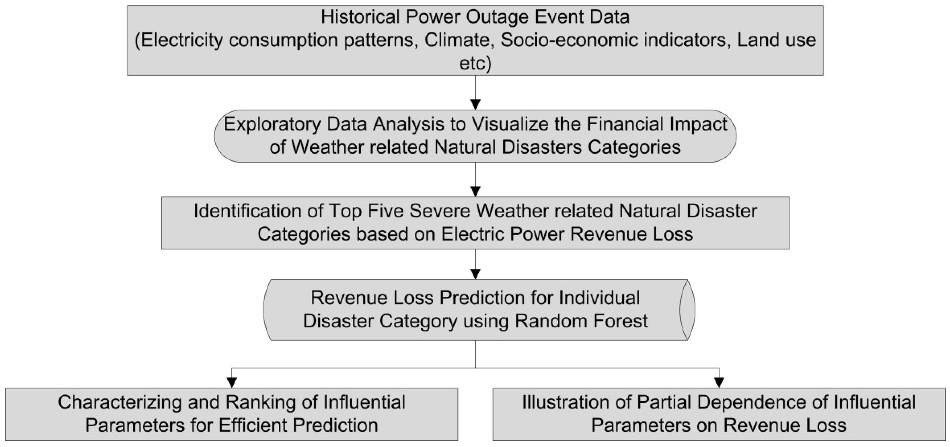
• An exploratory data analysis is presented to identify and lay the foundations of this research, leading to analyze the impact of top weather-related natural disaster categories on power outages;
• The top five most financially catastrophic weather-related natural disaster types are investigated where for each disaster category, the revenue loss prediction is performed;
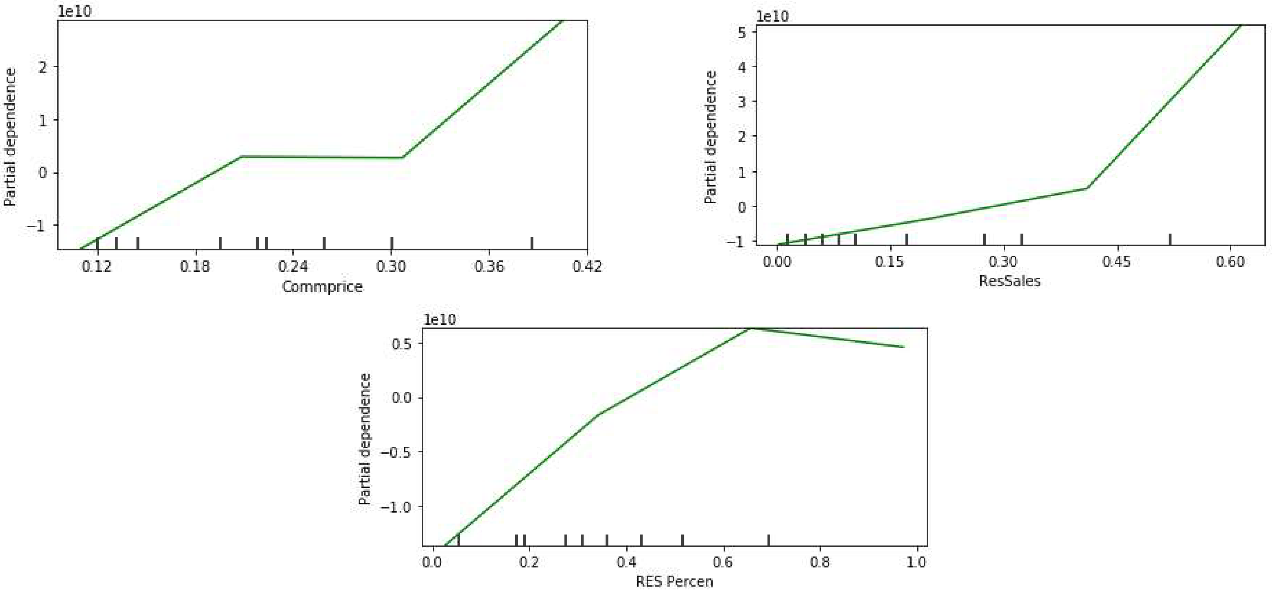
• Towards the efficient prediction of revenue loss, the 10 most influential parameters are identified and their relation with revenue loss is illustrated for each of the five disaster categories.

The paper is organized as follows: Section 2 presents the data and exploratory analysis. Methodology is explained in Section 3. The results and discussion are presented in Section 4 and Section 5, respectively. Finally, a conclusion is added at the end.

2. Exploratory Data Analysis

The United States has witnessed a large number of power outages in the past. Reliable data regarding historical power outages, collected from U.S. national agencies, are publicly available [36]. The data cover the information of 1534 outage events which happened over 17 years from 2000 to 2016 in 49 States. For each of the power outage events, the data include such information categories as electricity usage patterns, consumer strength, population density, climate annotation, social and economic indicators, and land area with a total of 51 parameters altogether.

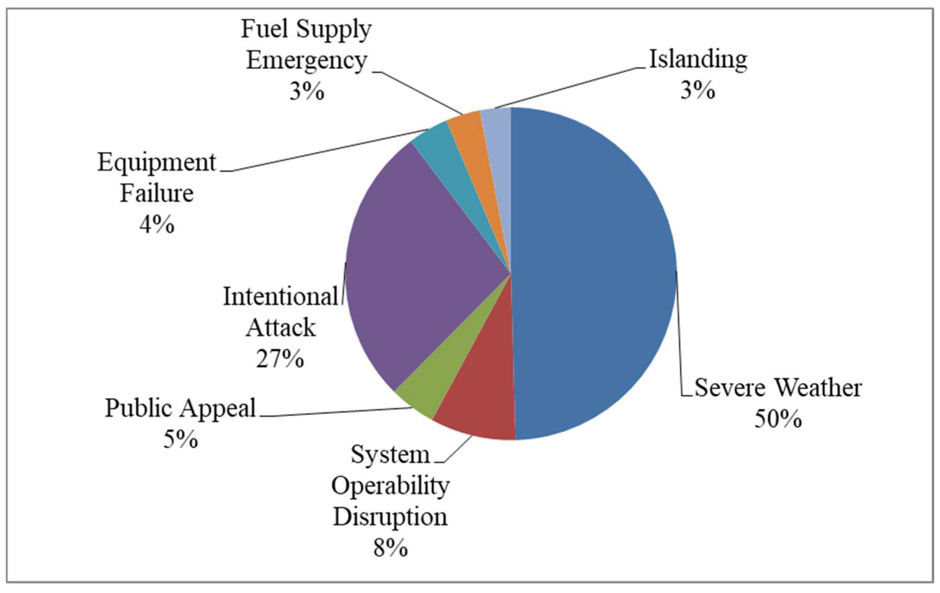
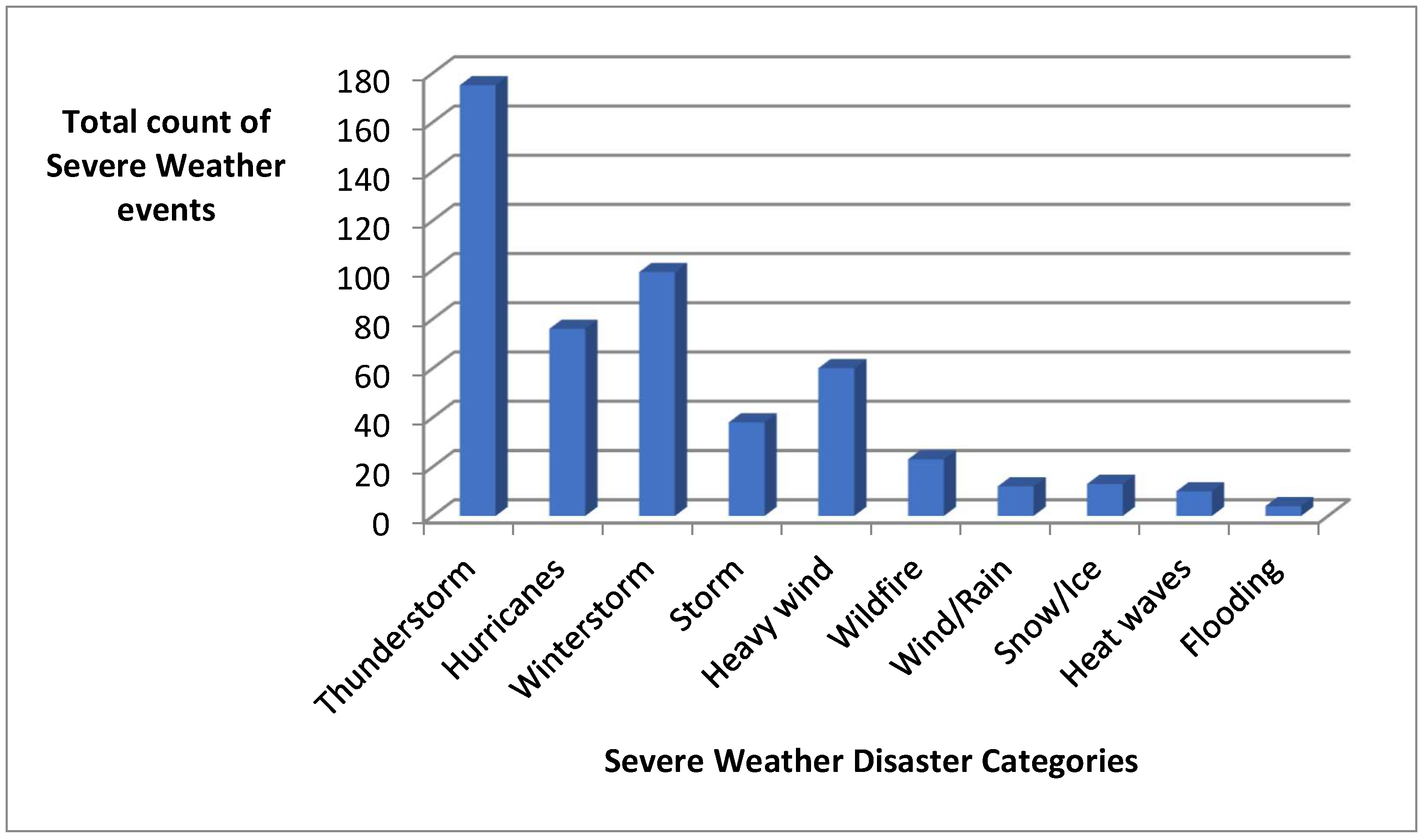
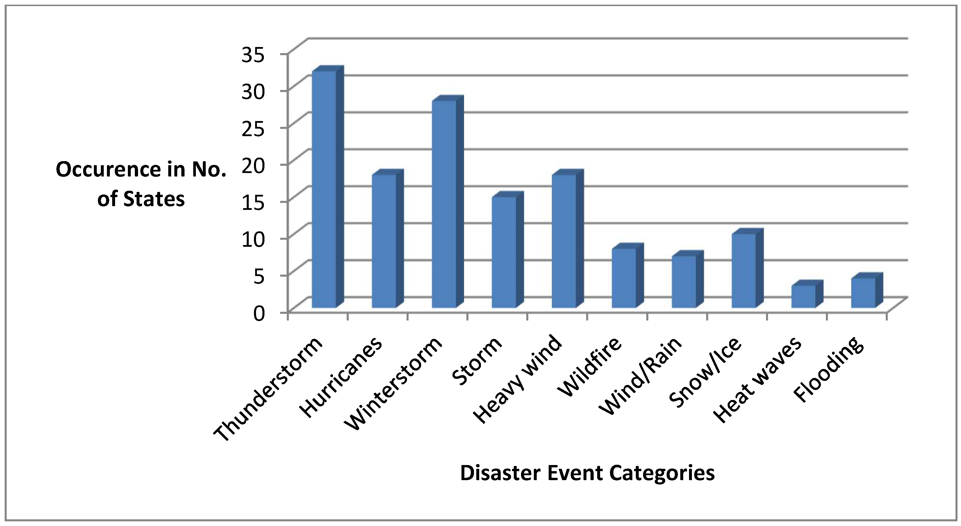
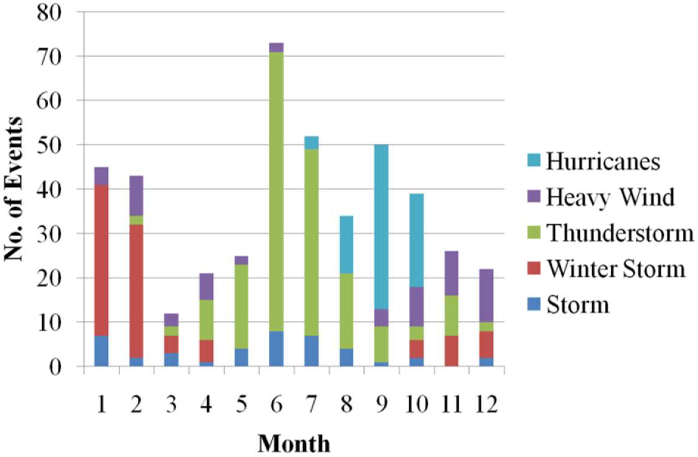
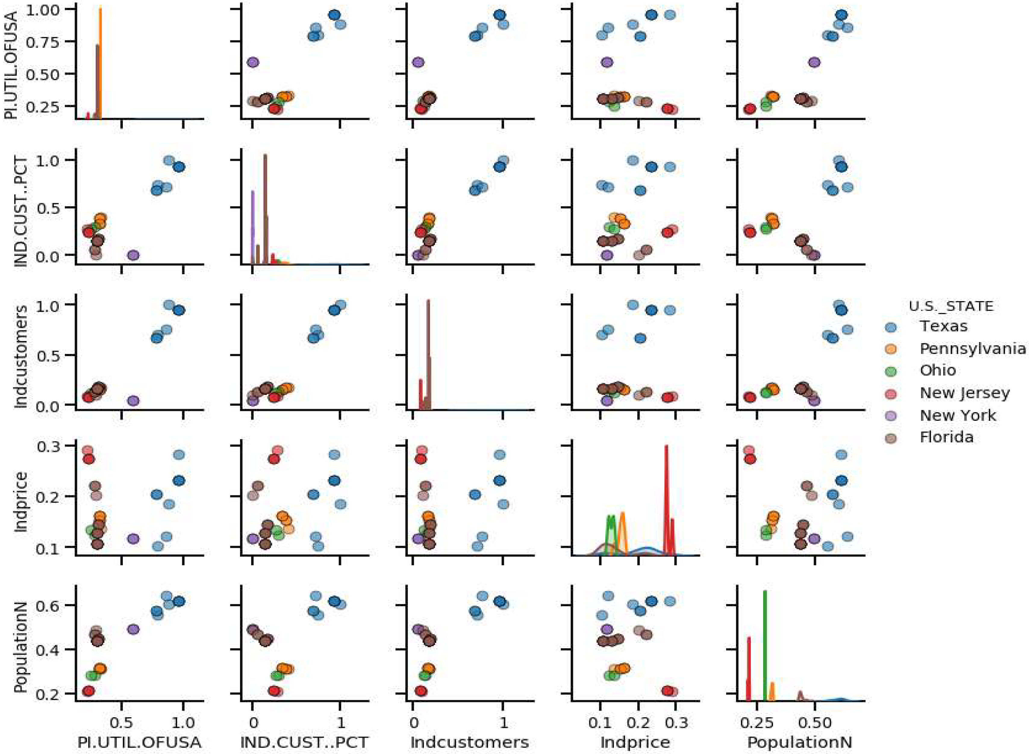
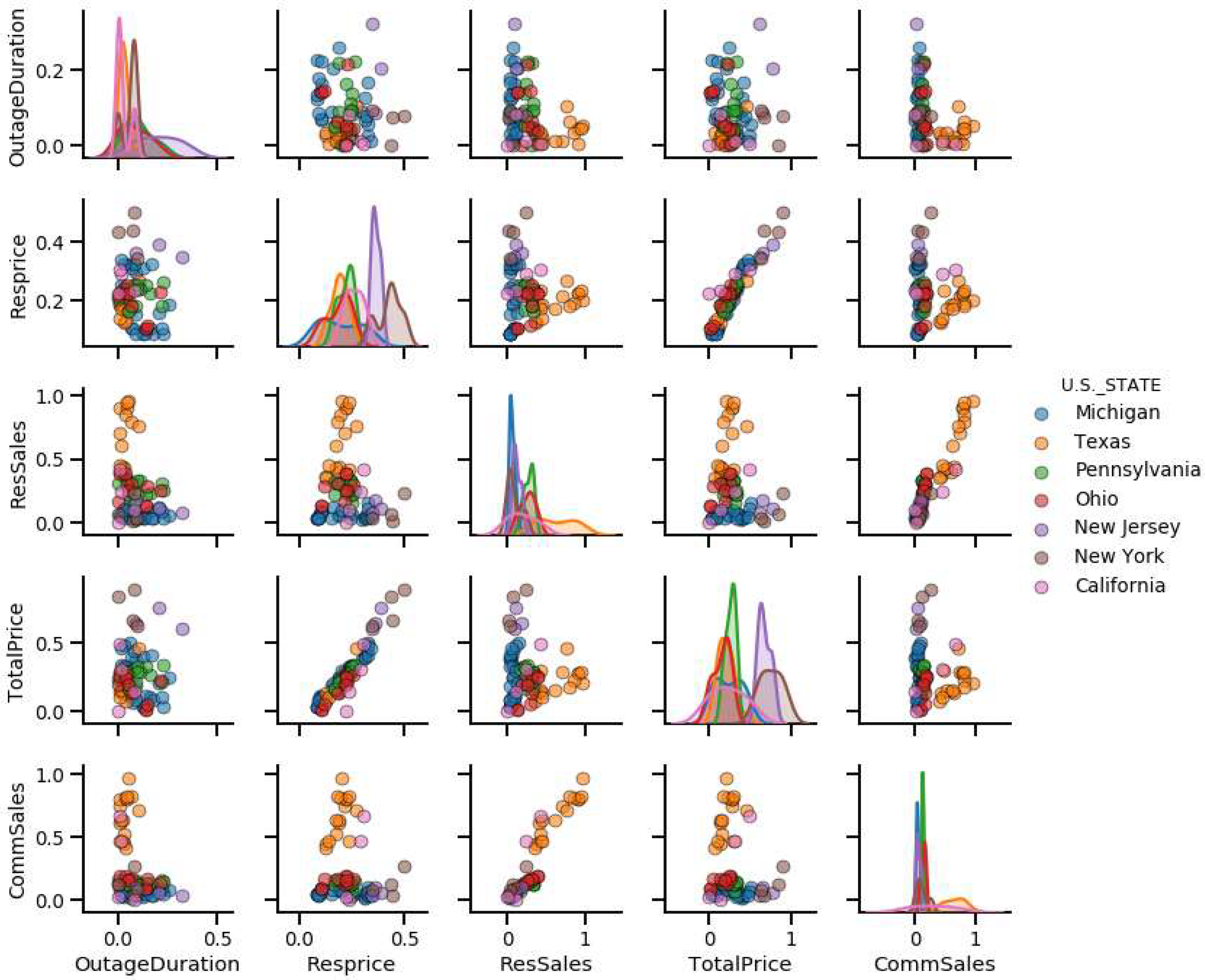
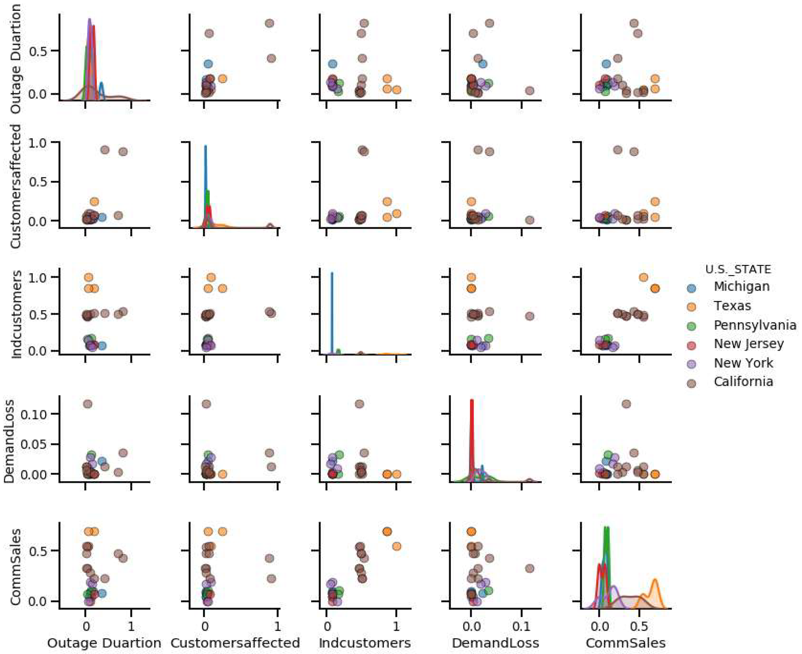
2.1. Visualization of Severe-Weather-Related Natural Disasters

Power outage data include the outage events which were triggered due to seven different explanations. Figure 1 shows the occurrence of different events in terms of percentages which caused the power outage. It can be observed that a weather-induced natural disaster was the reason behind half of the total events which occurred.

Most of the natural disasters were linked with severe weather conditions. Among those disaster types, the occurrence of a few was higher than the others, such as thunderstorms, hurricanes and winter storms. Figure 2 shows the frequency of the top 10 most frequently occurring disaster categories over the entire period of 17 years. It can be observed that all those disaster categories were related to severe weather conditions.

Next, we visualize in how many States a power outage event occurred which was related to a particular disaster category. Figure 3 illustrates the occurrence of individual disaster events in a total number of states of the U.S. It is observable that not only were the weather-induced disaster events the most frequent ones (as shown in Figure 1), but that their prevalence also existed across many States.

If we look carefully in Figure 2 and Figure 3, one can observe that the top five disaster categories remain the same with regard to occurrence as well as prevalence. Next, we find out the relevance of occurrences of those top five disaster categories with varying weather conditions over the entire year. The month-level frequency of these events is presented in Figure 4. It can be observed that thunderstorms and hurricanes were the reason behind power outage events during the summer season. Similarly, winter storms mostly caused power outages during the winter season. Looking at the statistics, it can also be observed that the reason behind 58% of all outage events is among the top five disaster categories.

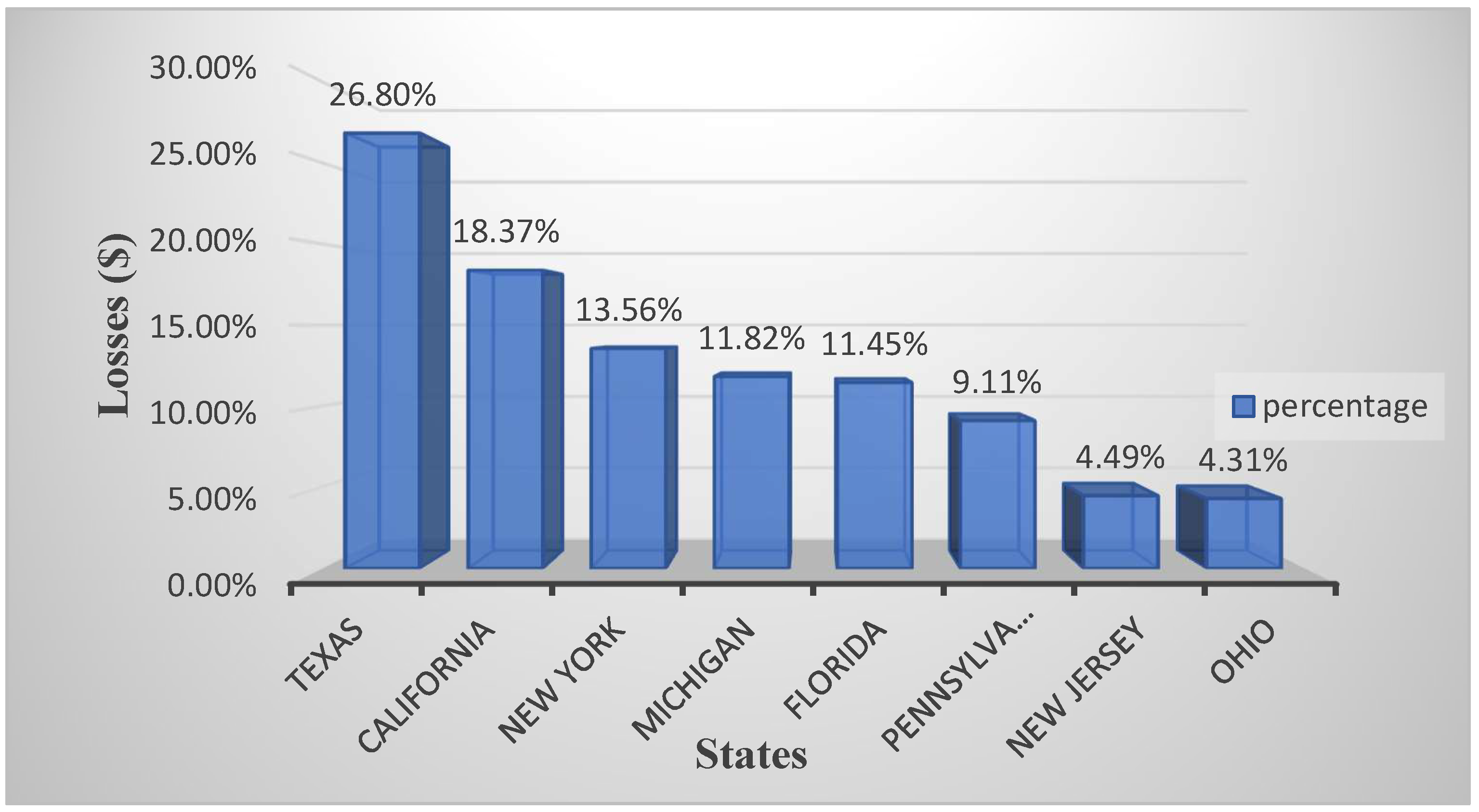
2.2. Visualization of Revenue Loss Associated with Weather-Related Natural Disasters

Power outages due to severe weather-related disasters cause electric power revenue loss for electricity-supplying corporations. The power outage data include the tariffs offered by electricity-supplying companies at the time of the outage event. Moreover, tariffs were distinguished among different customer categories, such as residential, commercial and industrial. The revenue lost during the power outage event due to the non-sale of electricity can be estimated using the tariff information and the total time of the outage. For example, for the residential sector, revenue loss was estimated as follows:

Residential revenue loss = Residential sale × Residential tariff × Total time of power outage

(1)

Similarly, revenue loss was computed in the commercial and industrial sectors as well. The total revenue loss during a power outage event was the sum of the losses of individual sectors. The data show there were seven different reasons which caused power outage events, including severe weather disasters. Figure 5 shows the reason for power outages and the corresponding total revenue loss in terms of percentages. It is evident that severe weather-related disasters were the reason behind more than two-thirds of the total revenue loss. As shown earlier in Figure 1, 50% of power outage events occurred due to severe weather-related disasters; however, the impact in terms of revenue loss was even higher, that is, up to 70%.

Having found that the major percentage of electric power revenue losses of 70% was due to severe weather disasters, we look into the revenue loss distribution among individual States of the U.S. It was found that more than 85% of the total revenue loss was witnessed by eight States of the U.S. Figure 6 shows the percentage distribution of the accumulated revenue loss in the top eight States (i.e., 85% of total revenue loss), among the individual States.

Finally, the revenue loss accumulated in the top eight States related to individual severe weather-related disaster categories is shown in Figure 7.

The exploratory analysis and visualizations reveal that weather-connected natural disasters triggered half of the total power outage events during 2000–2016, and also caused 70% of the total electric power revenue loss. The scope of this research is to analyze the impact of top severe weather-related disaster categories and to predict the consequent losses in revenue. Since only 15% of the total electric power revenue loss happened in 41 States, while the remaining 85% of revenue loss was borne by eight States, it is convincing as well as convenient to consider the data of eight States for further analysis and prediction. Therefore, further in the research, analysis and prediction are carried out based on the data of the eight most vulnerable States of the U.S., as shown in Figure 6.

3. Methodology

The visualization of severe weather-related disasters and electric power revenue loss in the exploratory data analysis section revealed that the many of the outage events were triggered because of the top few categories of disasters overall. Therefore, to confine the scope of the research analysis, the top five most catastrophic severe weather-related disaster categories are investigated and revenue loss prediction is presented.

For revenue loss prediction in the case of the occurrence of a severe weather disaster, machine learning (ML) algorithms were considered. ML algorithms are based on data-driven approaches to solve the problem. Therefore, it is critical to select the appropriate algorithm which is particularly suitable for the nature of the data. The dataset used in this research is diverse and multidimensional, and also includes outliers. Therefore, it is important to choose an appropriate machine learning algorithm which may perform well on such data. In the literature, several machine learning algorithms have been employed for different applications, such as support vector machines, random forest, decision trees, the artificial neural network, and linear models [12,35,37]. However, random forest (RF) has proved to be the best candidate, particularly in the case of non-linear data with high diversity and outliers, considering multiple research domains [12,17,35,38,39,40,41,42]. The overall flow chart of the research methodology is shown in Figure 8.

3.1. Random Forest Prediction Algorithm

Random Forest is an ensemble learning technique originally developed by Brieman [43] and is used for both classification and regression purposes. The key advantage of this algorithm is that it is a non-parametric technique which can handle the noise and non-linearity in data very well. It has high predictive accuracy and does not require any stiff rules. The number of the trees or estimators plays a key role in the prediction process. The efficiency and accuracy of the model can be improved by selecting the optimum number of trees. According to general observation and also in our model, it is pragmatic that the higher number of trees, the greater accuracy in prediction results. Concretely, RF is a simple regression process in which it takes the split of data for training and testing purposes and minimizes the error on the data with the selected number of trees. It has fast convergence time and handles the noisy data easily which makes it superior over other algorithms, specifically considering the data used in this research.

3.2. Performance Evaluation Metrics

The aim of this research was to predict the electric power revenue loss associated with power outages caused by any of the top five severe weather-related natural disaster categories. Therefore, revenue loss was the response variable or output parameter to be predicted by the algorithm, while the rest of the parameters were used as input parameters. To evaluate the prediction results, the following evaluation and analysis parameters were measured.

3.2.1. Prediction Error

Prediction error tells the difference between the actual value and the predicted value. To evaluate the fit of the model, different kinds of errors were considered, such as mean absolute error (MAE), mean absolute percentage error (MAPE) and root mean square error (RMSE). The mathematical expressions of these errors are as follows:

$$RMSE\hspace{0.17em}=\sqrt{\frac{{\displaystyle \sum _{i=1}^n{\left(y_i-p_i\right)}^2}}{n}}$$

(2)

$$MAE\hspace{0.17em}=\hspace{0.17em}\frac{{\displaystyle \sum _{i=1}^n\left|y_i-p_i\right|}}{n}$$

(3)

$$MAPE\hspace{0.17em}=\frac{1}{n}\hspace{0.17em}{\displaystyle \sum _{i=1}^n\frac{\left|y_i-p_i\right|}{y_i}}$$

(4)

where p_i represents the predicted value, y_i represents the actual value, and n represents the total number of observations.

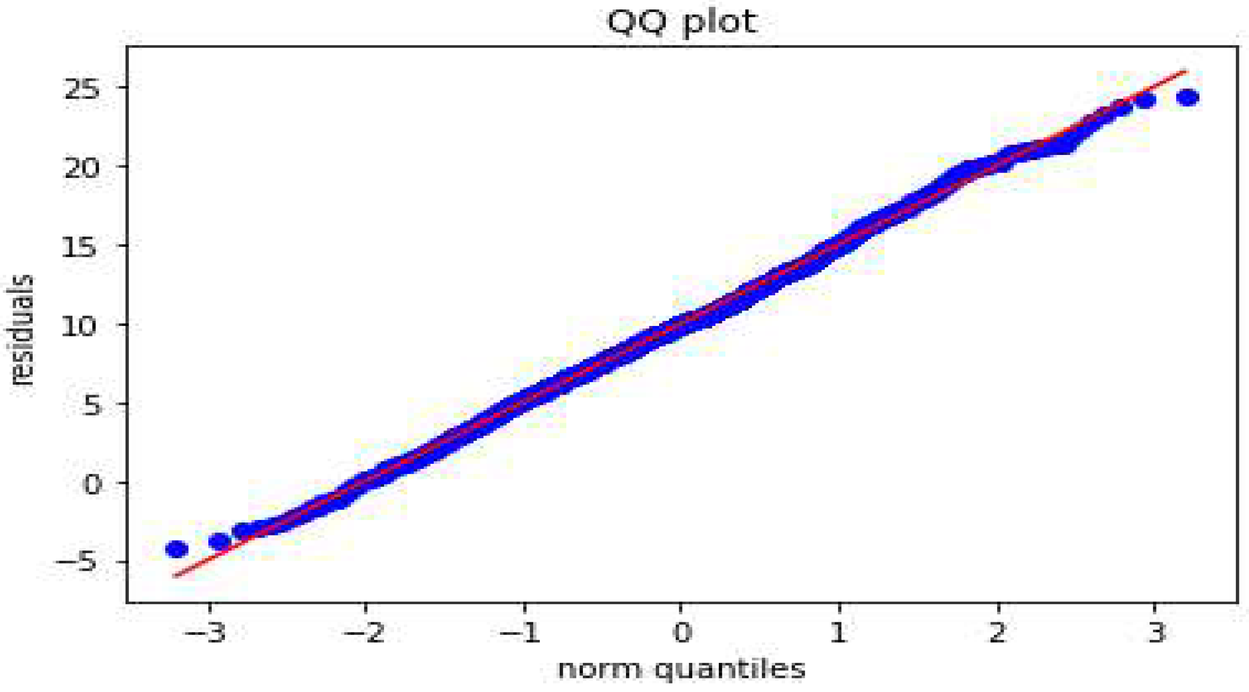
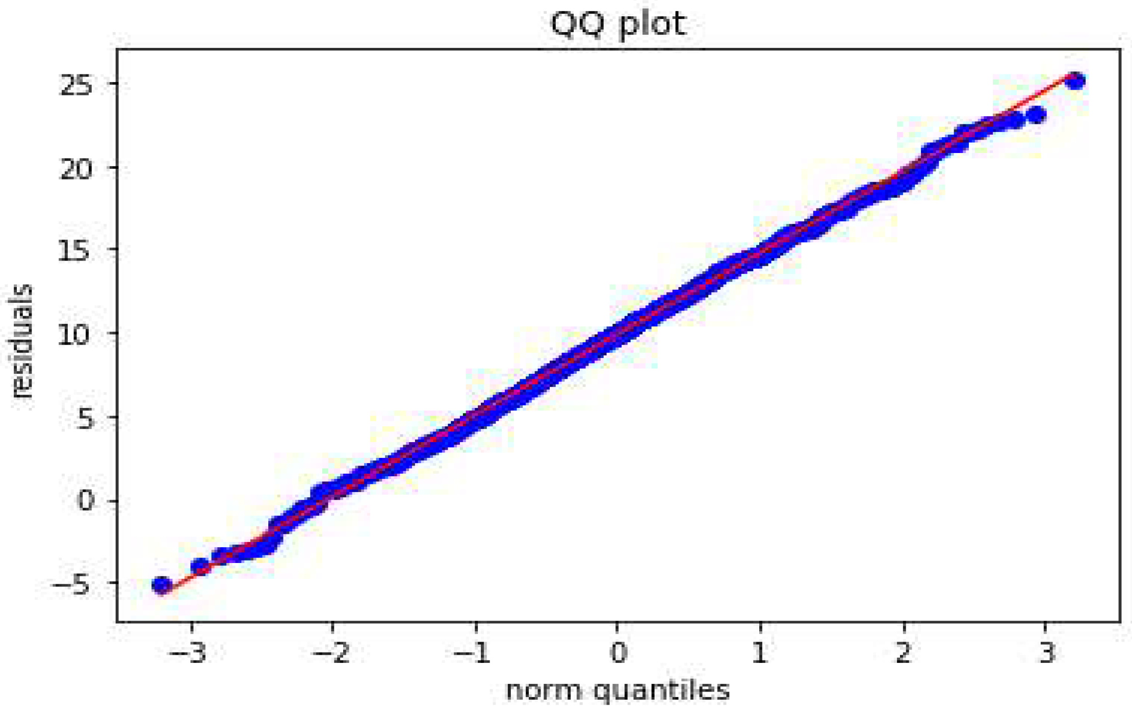
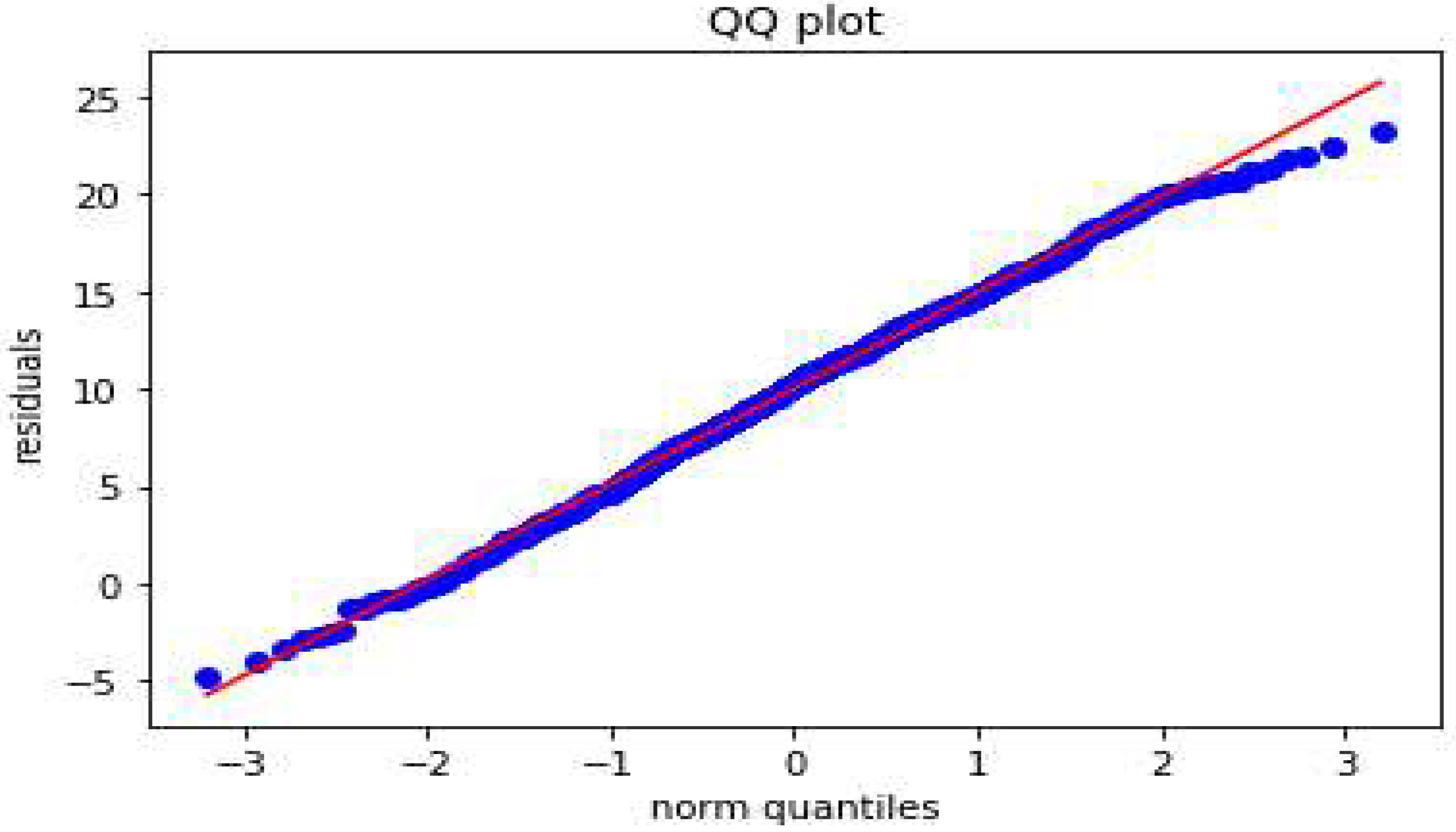
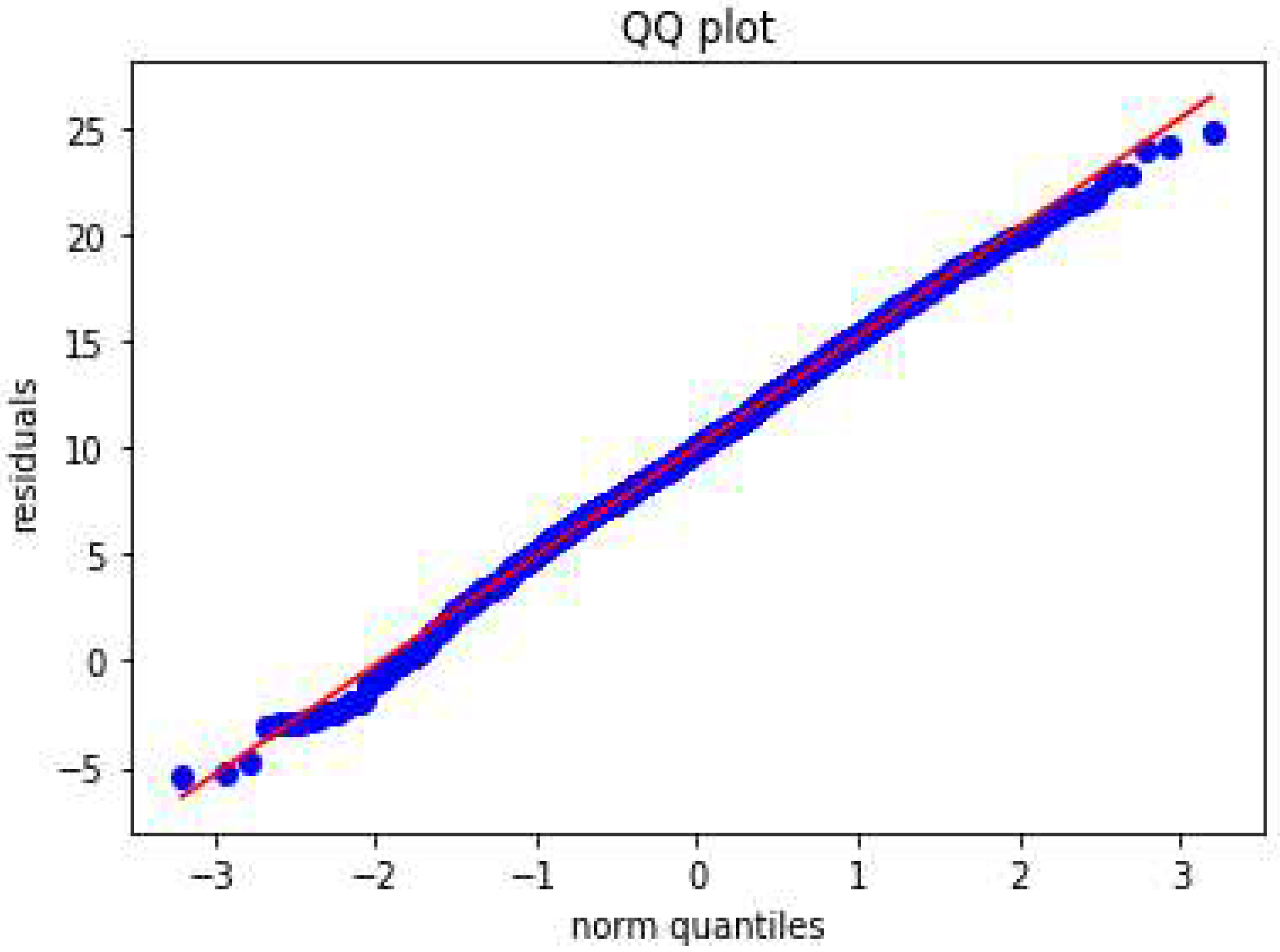
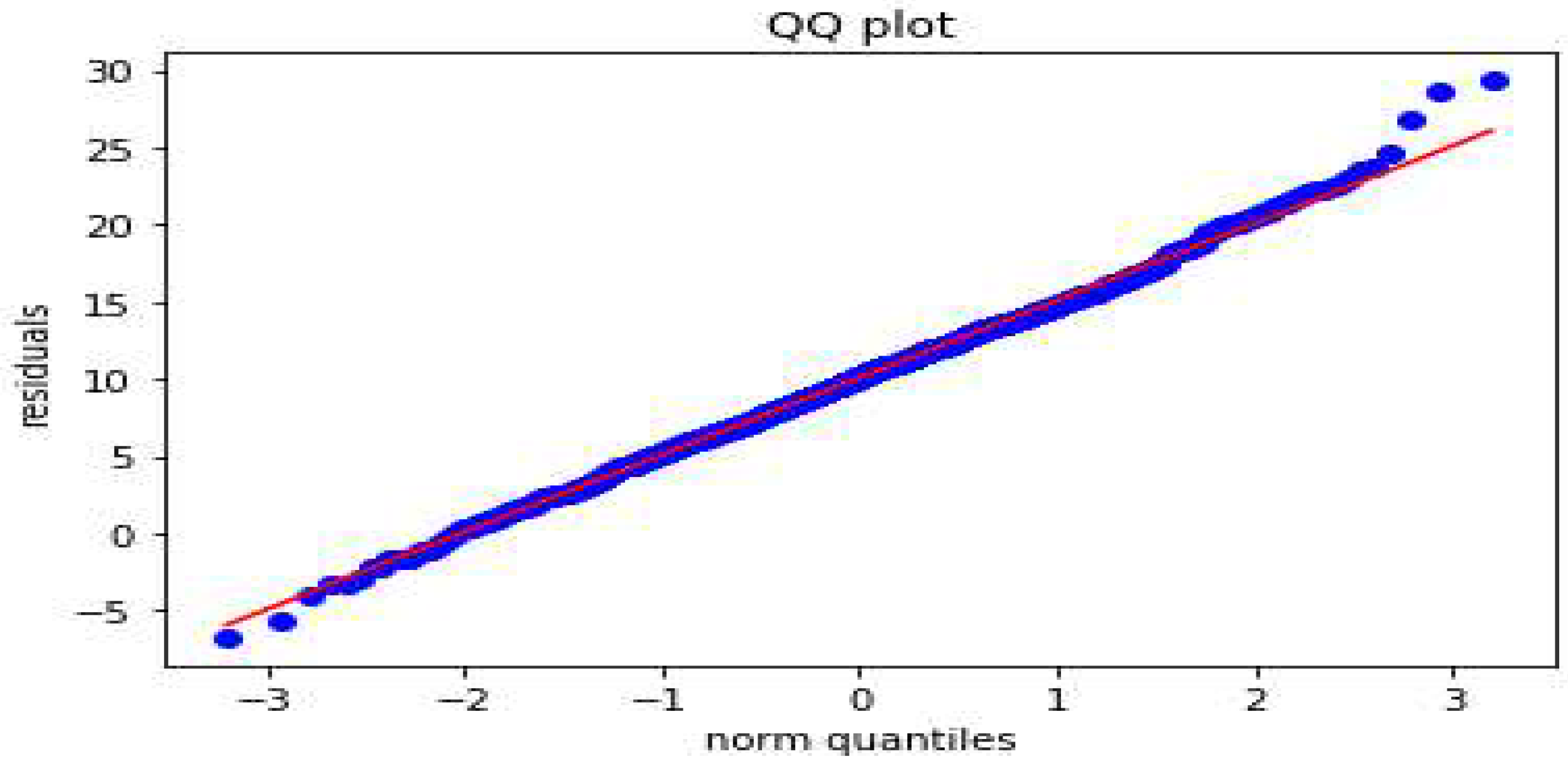
3.2.2. Quantile–Quantile (QQ) Plot

A QQ plot is another approach to see similarities between the data and a specific probability distribution. It typically checks whether the data set is normally distributed or not. It is different from histograms and pie charts because both the axes in QQ plots are used to show the quantiles. Usually, the sample data are taken on the vertical axis, and the desired probability distribution on the horizontal axis. The plot shows whether the data are distributed according to the desired probability distribution, and as a result, data samples are distributed along a 45-degree line. The graphs with normal distribution usually have a symmetric curve and are rarely skewed left or right.

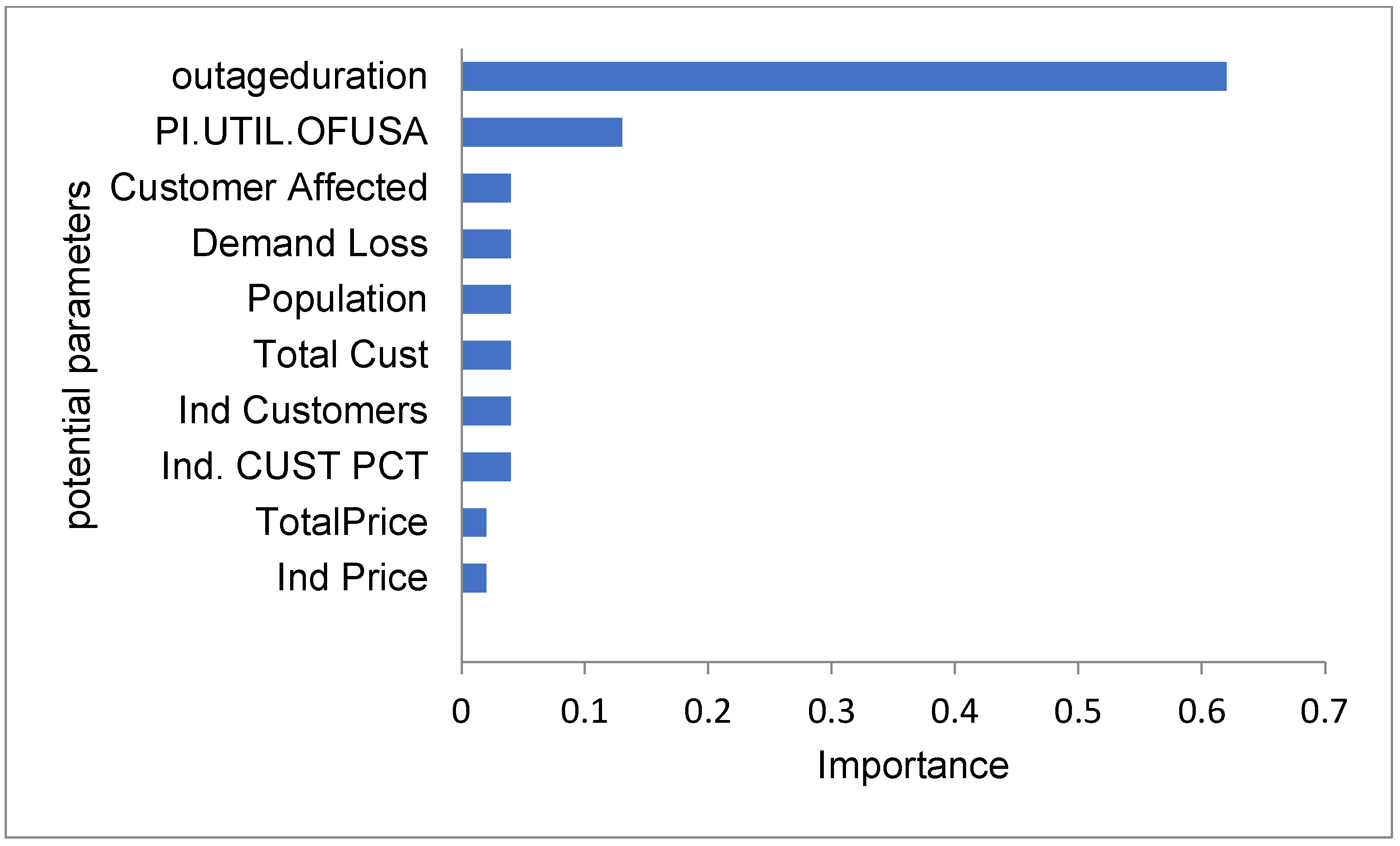
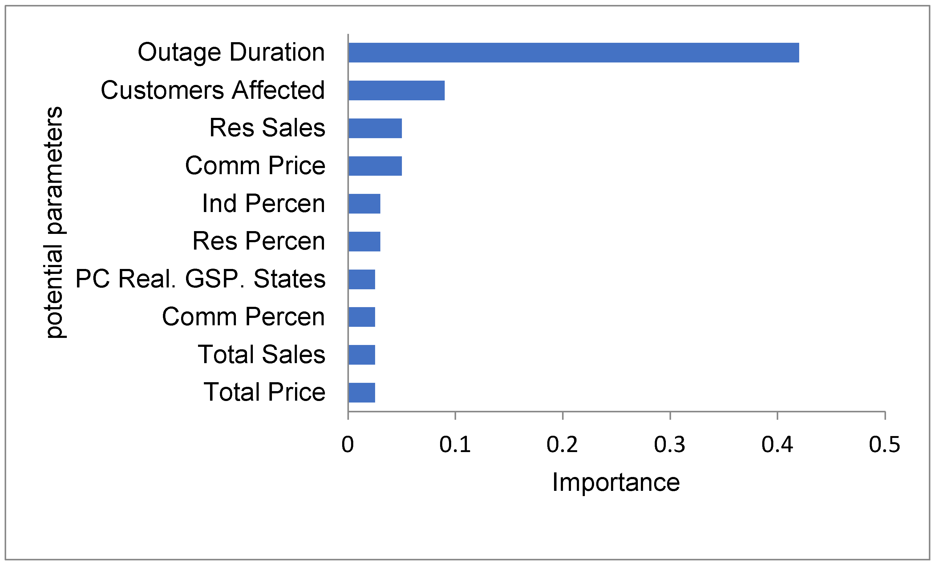
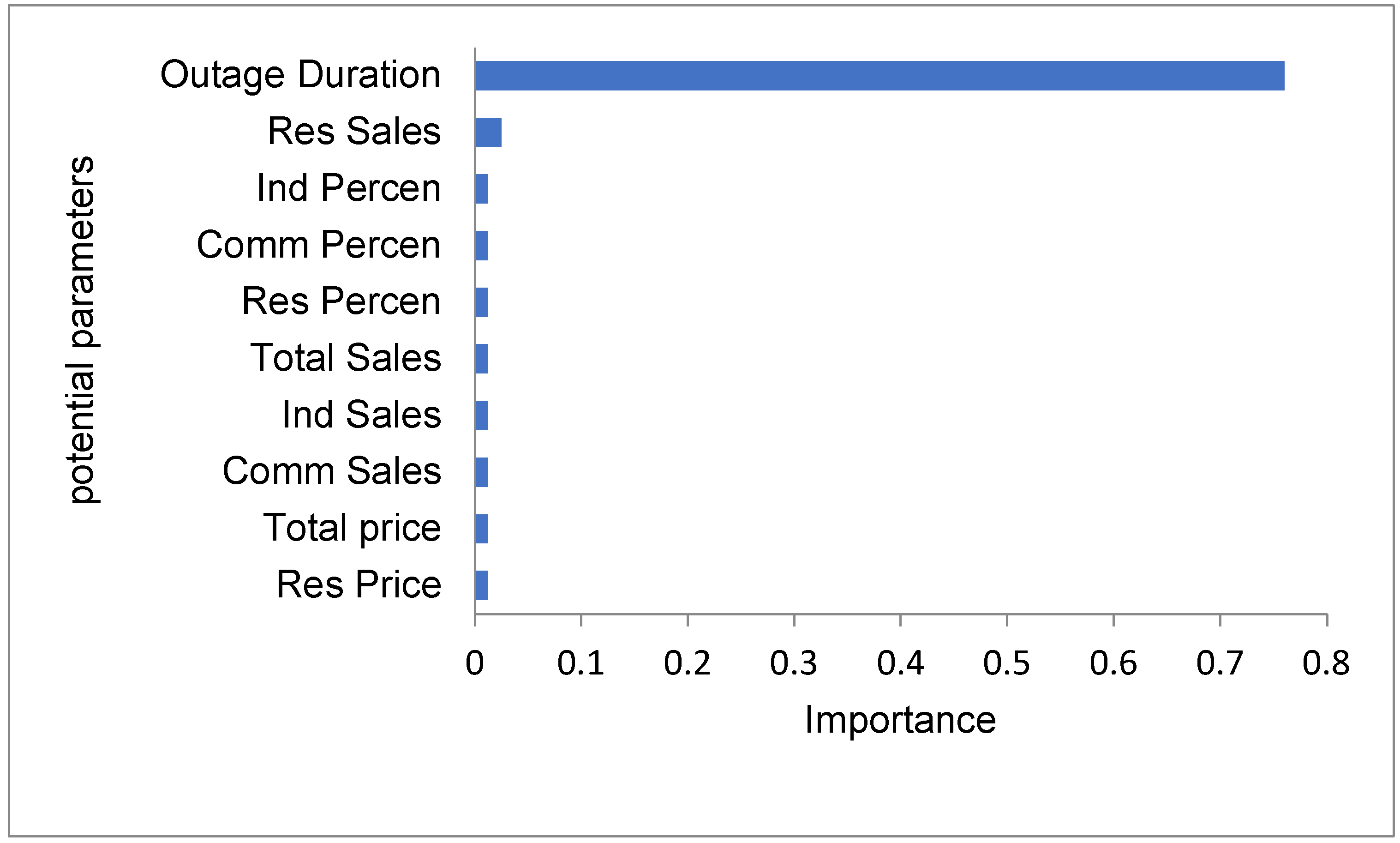
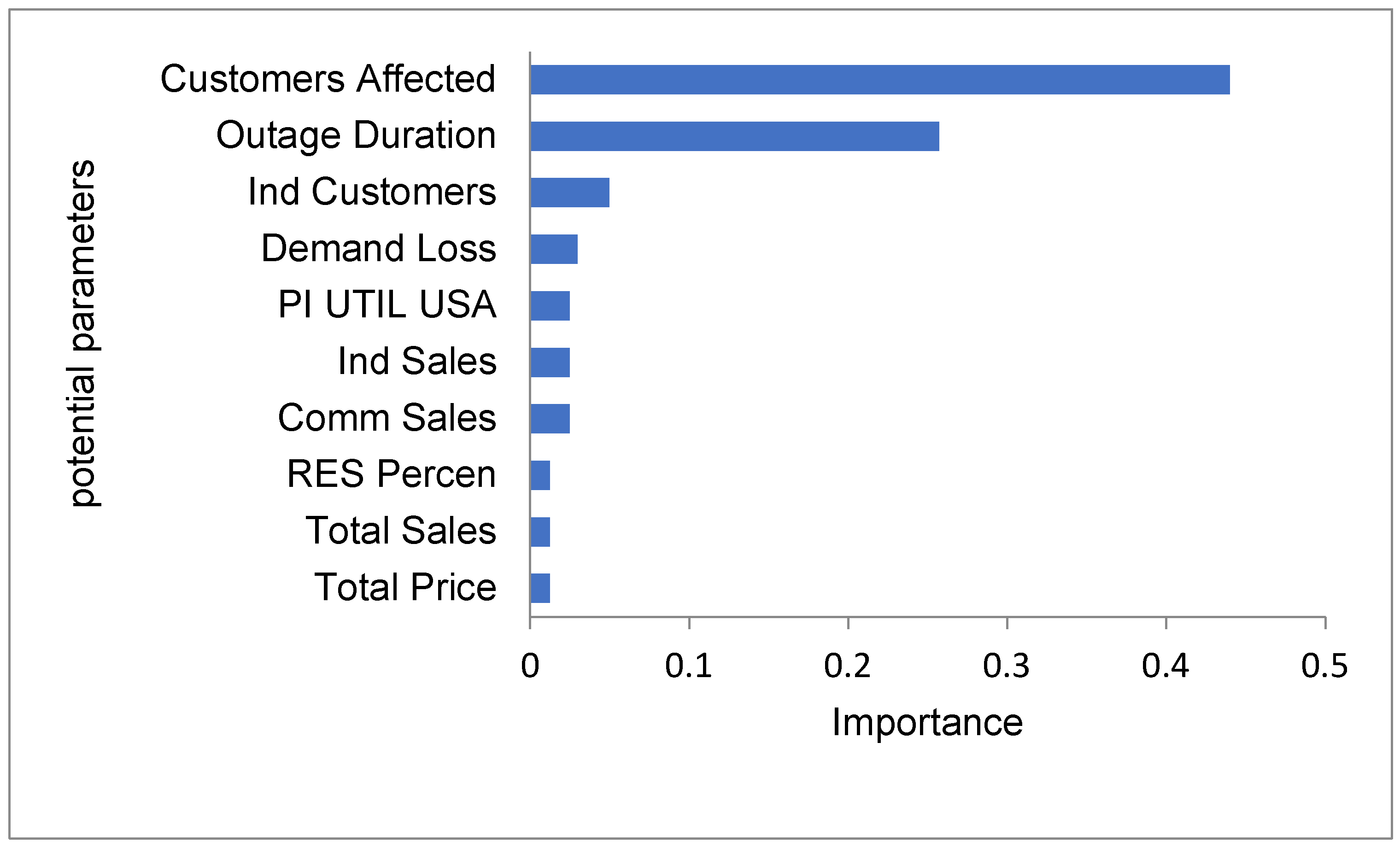
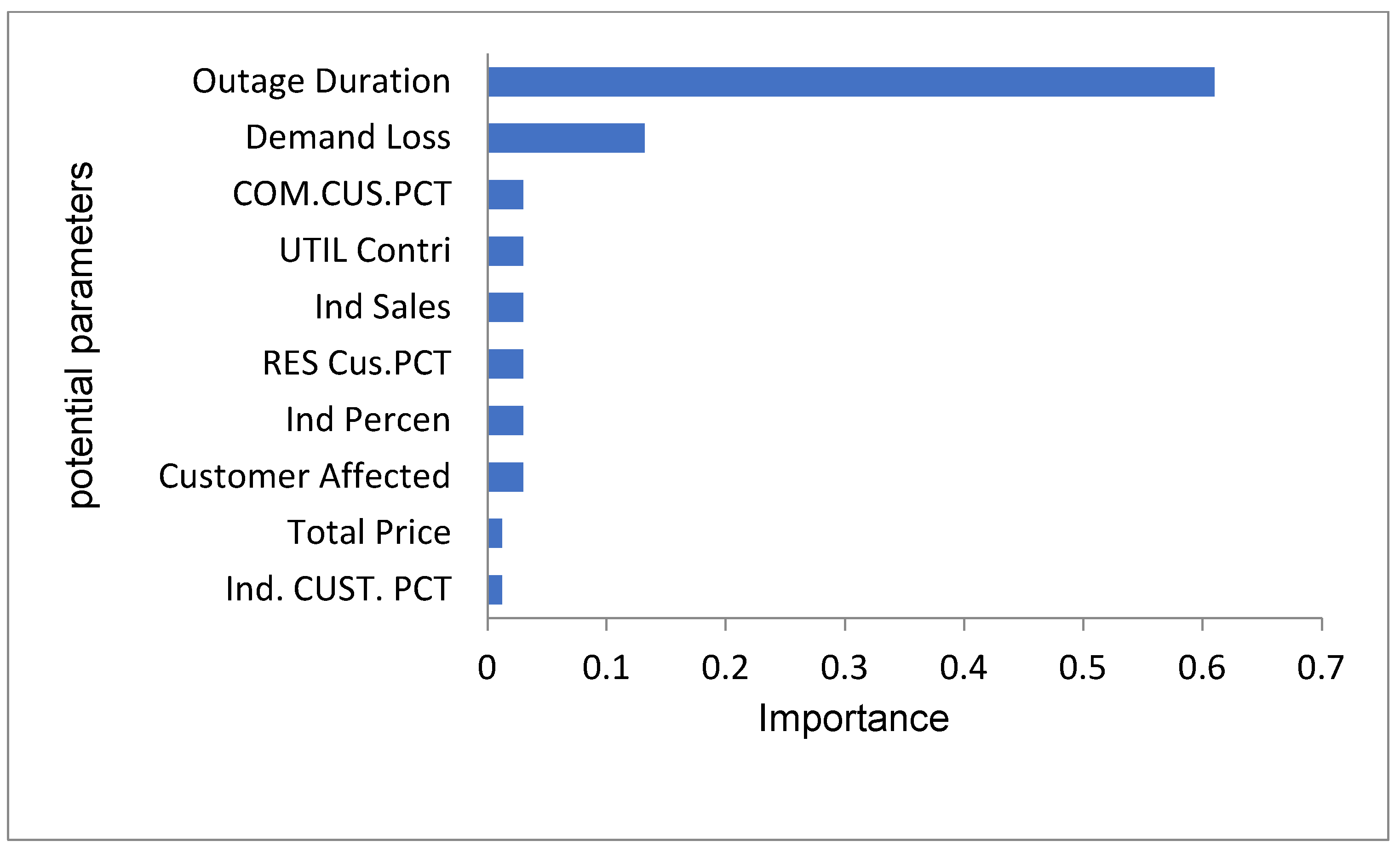
3.2.3. Influential Feature Ranking

Feature ranking is used to identify the most influential parameters in the data which contribute for the efficient prediction by of the output variable. The influence of each feature towards electric power revenue loss is presented in terms of normalized importance of the feature used in the algorithm.

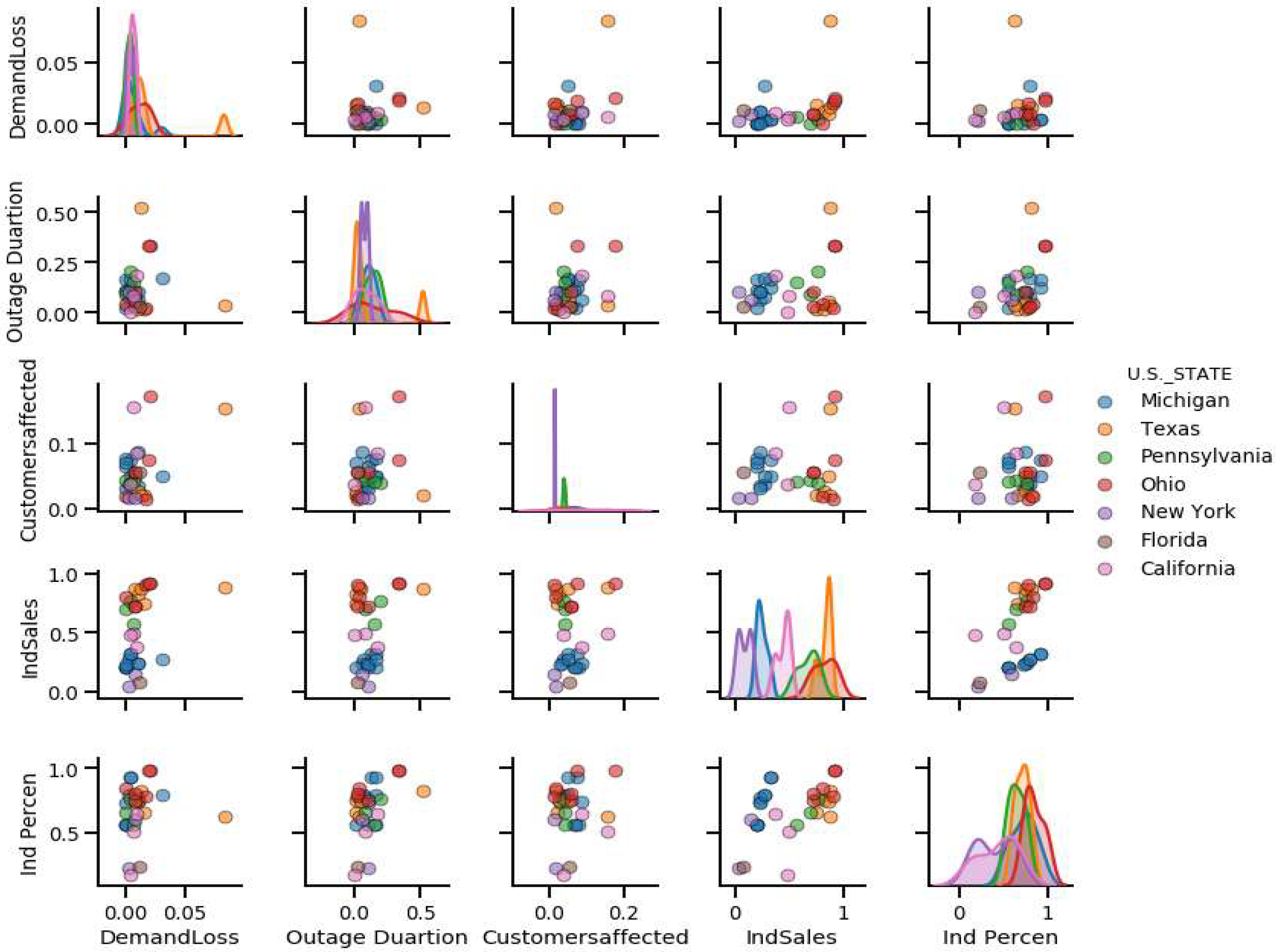
3.2.4. Correlation Plot

The correlation plot is used to interpret the relation between different variables in a data set. It is a convenient way to find the linearity or non-linearity in the data. These types of plots are mostly used to create a link and association among the variables present in the data.

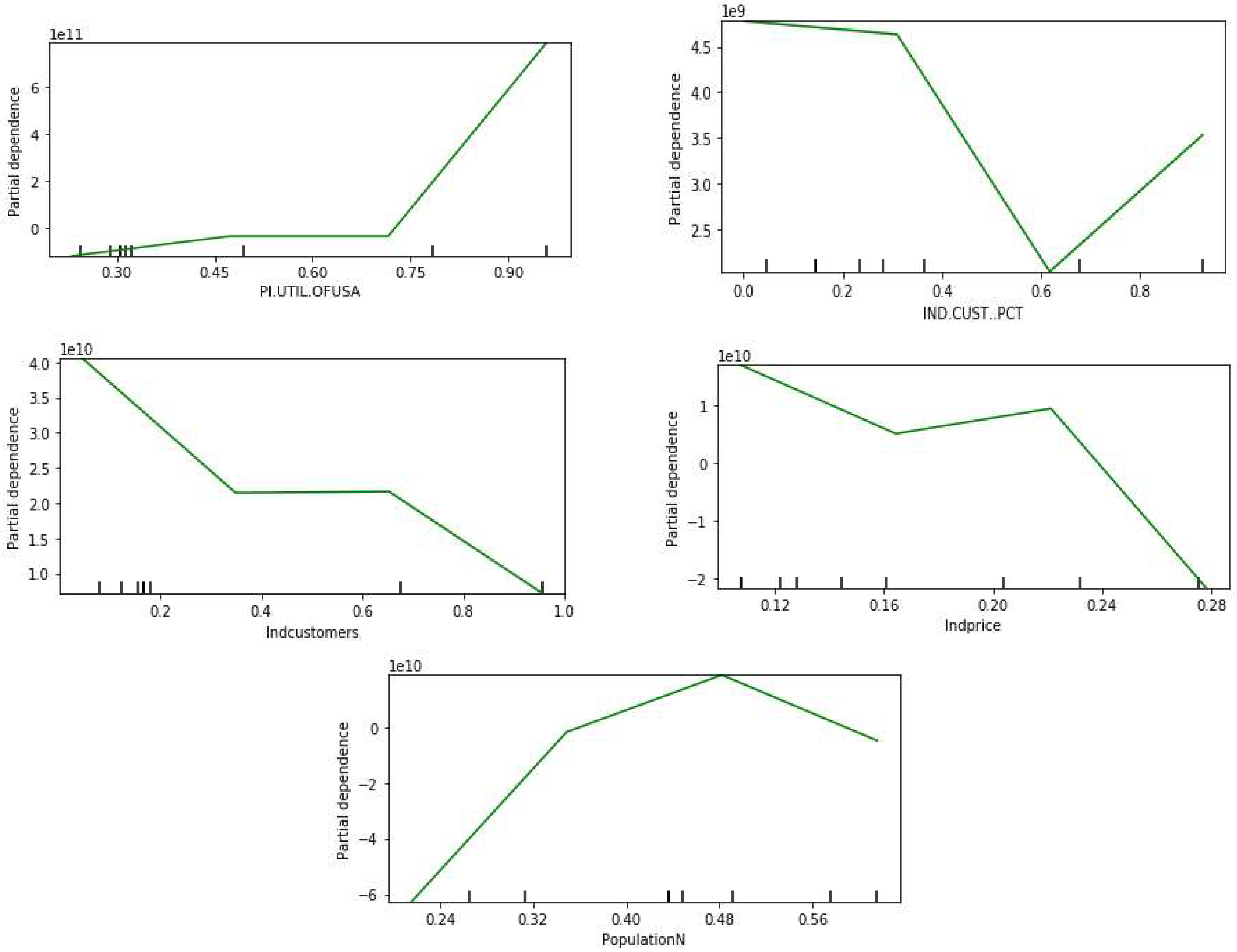
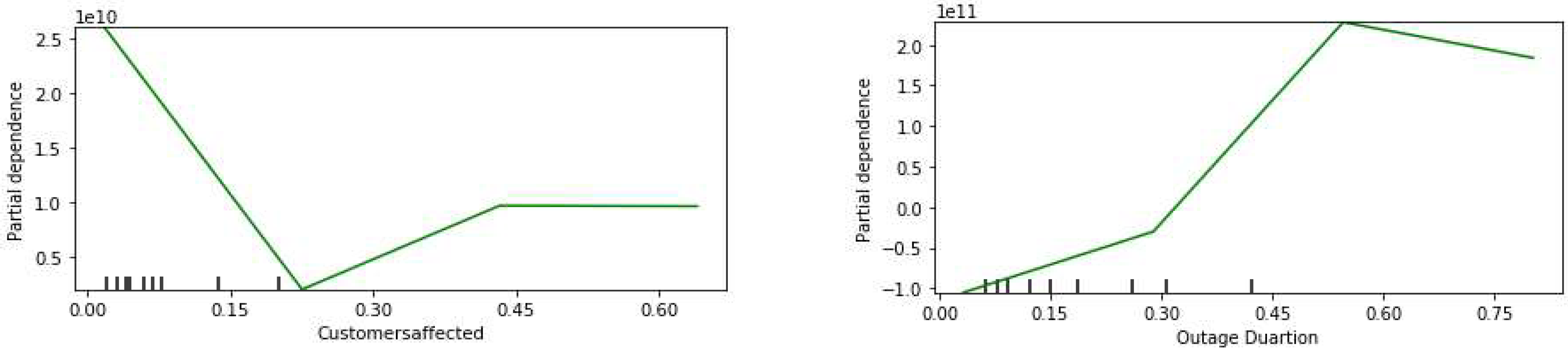
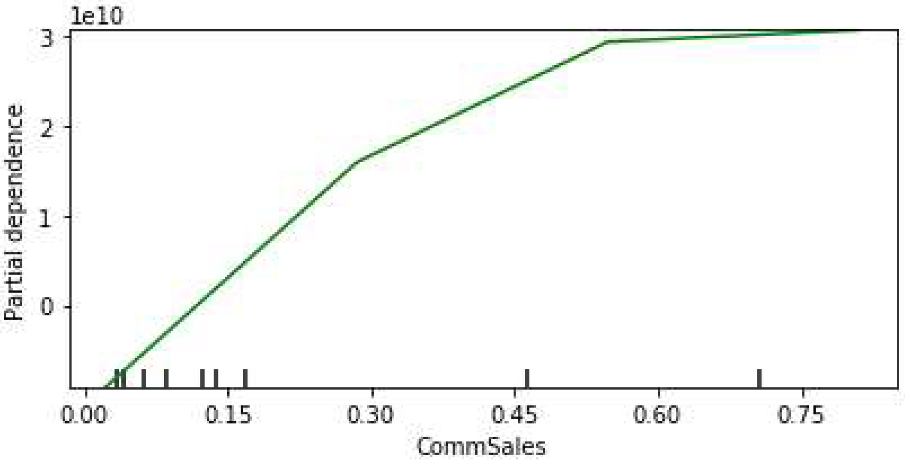
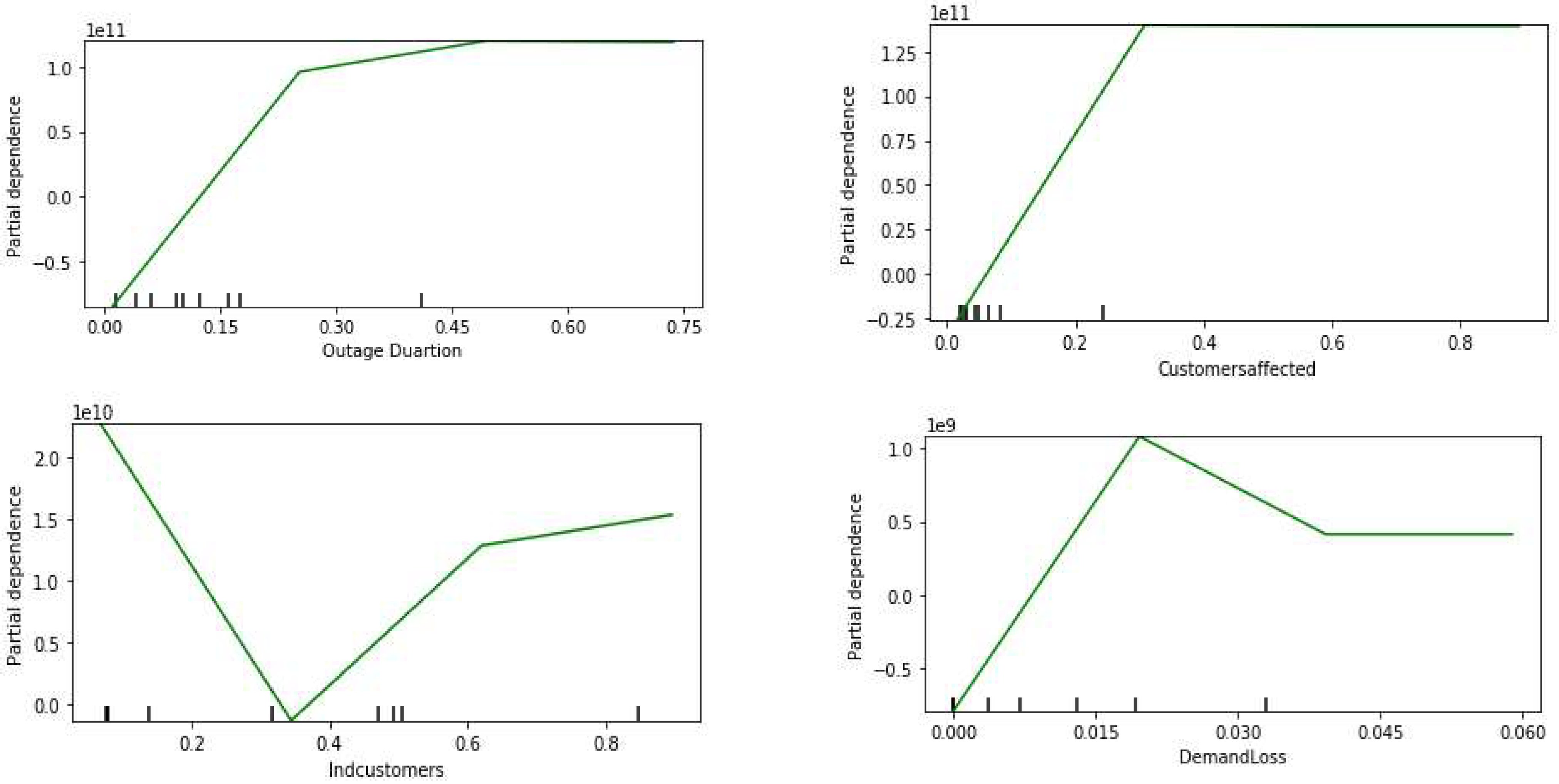
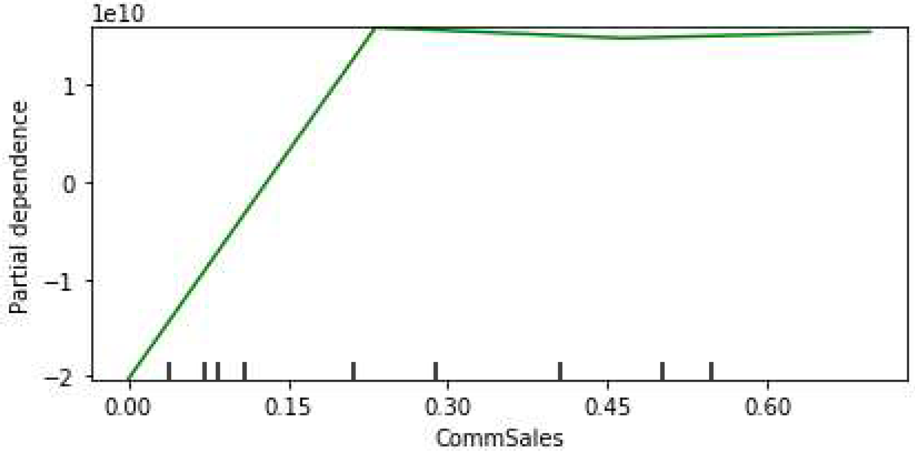
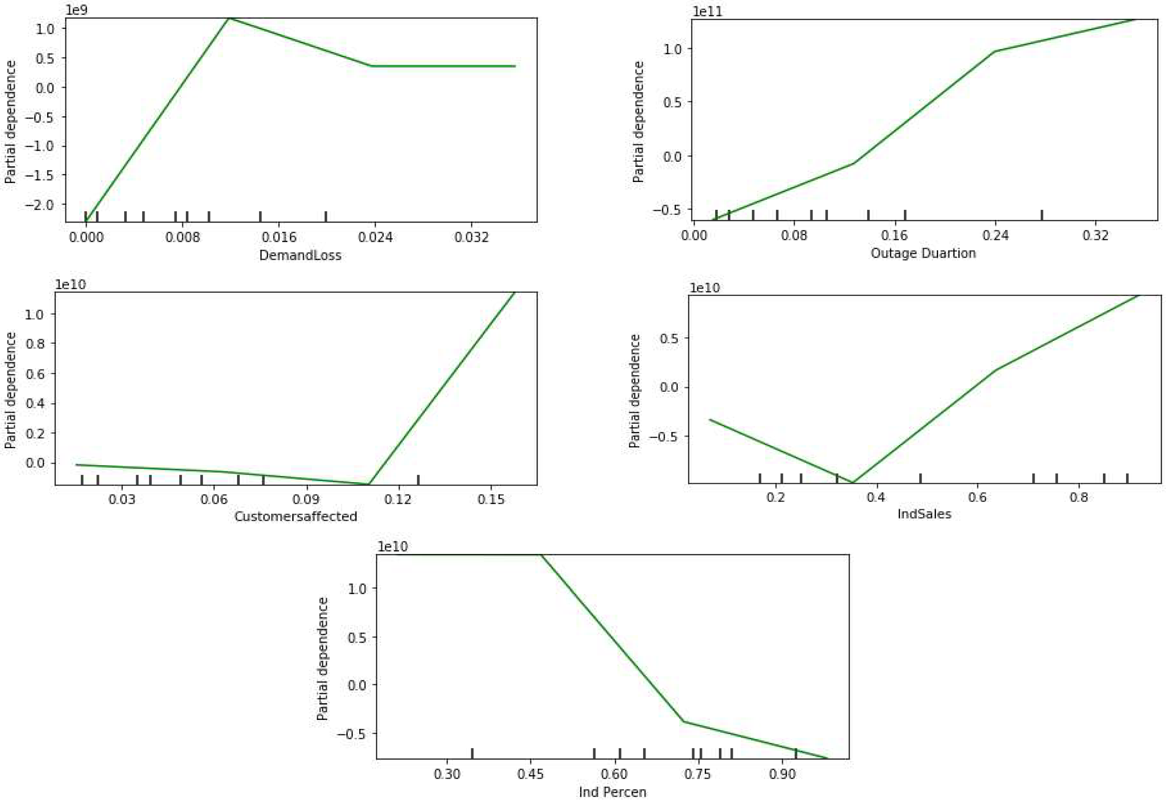
3.2.5. Partial Dependency Plot (PDP)

A Partial dependence plot shows the marginal relationship between the response variable and predicted variable to show whether the model is linear, monotonic, or of any other non-linear kind [44]. Sometimes the value of a PDP is negative, which shows that the predicted variable would have been less than the actual amount. Mathematically, it can be obtained as follows:

$$f_{j\left(x_j\right)}=\raisebox{1ex}{$1$}\!\left/ \!\raisebox{-1ex}{$n$}\right.{\sum }_{i=1}^n{f}_{j\left(x_j-x-j{,}_i\right)}$$

(5)

where f is the estimated response, n is the total number of observations in training data, and the average value of the variable over the marginal distribution is obtained.

4. Results

The revenue loss prediction due to the top five individual disaster categories is presented and discussed in this section. For each disaster category, detailed results are presented and discussed, including prediction errors, the QQ plot, important feature characterization, correlation plots between the top five important features, and the PDP of the top five features.

4.1. Hurricanes

In this sub-section, the results of revenue loss estimation due to hurricanes are presented. The power outage data related to the hurricane disaster category were used to perform the experiments. Employing the random forest algorithm, different numbers of trees were selected and results recorded.

Table 1. Revenue loss prediction errors due to hurricanes.

Experiment	No. of Trees	MAPE	MAE (USD)	RMSE (USD)
1	50	23.45	23,079,835,627	28,026,732,162
2	80	34.85	30,018,823,161	33,616,564,460
3	100	34.91	30,212,456,847	36,824,097,170
4	200	30.48	27,327,924,177	36,868,394,234
5	300	27.84	26,556,687,363	37,152,012,173
6	400	28.31	26,786,049,438	37,800,187,377
7	500	29.69	27,269,116,911	37,114,244,997

shows the revenue loss prediction errors for hurricanes. The MAE and RMSE of revenue loss are expressed in USD and rounded to an integer value. It can be observed that the minimum MAPE was achieved with 50 trees, while errors increased when increasing the number of trees.

Figure 9 shows the QQ plot for the hurricane data prediction results. It can be observed that residuals fall along the 45-degree line, which reveals that the random forest model captures the data variability well.

Figure 10 shows the top 10 features ranked for the correct prediction of revenue loss. The outage is the most important feature with a normalized importance of 0.62, while the second influential feature is the utility sector income as percentage of the total income of the U.S. The six more features down the line have equal normalized importance. The variable ranking is based on the mean decrease for out-of-sample prediction accuracy.

Figure 11 shows the correlation plot between the top five influential features. The plots along the 45-degree line show the mass distribution of a single feature. The remaining plots illustrate the inter-feature correlation. It is observable from scatter plots in the right-most column of the figure that the population parameter has a positive correlation with the rest of the four influential features. Similarly, the contrary case of no correlation can be observed by looking at the scatter-plot between the industrial price feature and the percentage utility of the U.S.

The individual partial dependence plots for the top influential features are shown in Figure 12. It can be observed that industrial customers and industrial tariff prices have a negative linear relation with revenue loss in general, except in the middle range where revenue loss increases with a small increase in the price. Similarly, the percentage of the utility industry in the income of the U.S. and the population has a positive relation with revenue loss.

4.2. Winter Storm

In this section, the revenue loss prediction is shown using the outage data associated with winter storms. Different values for the number of trees in a random forest implementation were selected and results recorded.

Table 2. Revenue loss prediction error of different experiments for the winter storm category.

Experiment	No. of Trees	MAPE	MAE (USD)	RMSE (USD)
1	50	29.69	32,220,838,997	41,084,191,702
2	80	30.13	33,415,595,609	41,830,421,202
3	100	31.11	33,999,830,403	42,091,161,381
4	200	26.12	30,359,905,448	39,364,991,165
5	300	26.89	31,464,230,122	40,729,734,176
6	400	26.26	31,164,528,874	41,096,929,311
7	500	26.35	30,986,271,677	40,636,022,029

shows the revenue loss prediction error results for winter storms. The minimum error was recorded with 200 trees.

The QQ plot for the winter storm data prediction results is shown in Figure 13, which reveals that the random forest model captures the data variability well, since the residuals fell along the diagonal line.

Figure 14 shows the 10 most influential parameters towards an accurate prediction of revenue loss. The outage duration has a normalized importance of 0.46, and this is the highest. The second most important feature is the number of customers affected. Down the list, there are different parameters which contributed equally for prediction.

Figure 15 illustrates the performance analytics graph showing the inter-feature relationship of the top five features. The plots along the off-diagonal direction represent the density distribution of individual features.

Figure 16 shows the individual partial dependence plots for the top five influential features. It can be seen that the residential sales and the commercial price have a positive relation with the revenue loss. A similar relation can be observed for outage duration and the residential customers’ percentage up to the 60% range; however, the relationship is inverted in the higher range.

4.3. Thunderstorms

Thunderstorms was the third most catastrophic natural disaster category related to power outages and the associated electric power revenue loss. The error results by choosing a different number of trees for the RF algorithm are shown in

Table 3. Revenue loss prediction error of different experiments for the thunderstorm category.

Experiment	No of Trees	MAPE	MAE ($)	RMSE ($)
1	50	34.64	27,243,171,092	42,976,400,445
2	80	36.27	27,594,272,395	42,609,631,917
3	100	35.18	26,952,676,148	42,482,427,053
4	200	35.27	26,748,282,945	41,787,071,287
5	300	34.77	26,367,527,269	41,708,198,459
6	400	35.22	26,644,653,509	41,781,040,877
7	500	35.52	26,713,157,021	41,810,251,294

. It can be observed that there was not any significant improvement by increasing the number of trees, and the result with 50 trees was good enough.

Figure 17 shows the quartile–quartile plot for the thunderstorm data. The deviation between the normal quantile and the residual can be observed in the top-right corner, that is, the right tail of the distribution.

The top-ranked 10 influential features for revenue loss prediction are shown in Figure 18. The outage duration is the most important feature and it stands out with a normalized importance of 0.76. The residential sale is the second with 0.02, while the rest of the features have equal importance of 0.01 only. Hence, the outage duration is the most important and single important feature for electric power revenue loss prediction.

The correlation plot between the top five important features for thunderstorm-based revenue loss prediction is shown in Figure 19. The positive correlation between individual features can be observed in the plots having diagonal distribution of data, such as between commercial sales and residential sales.

The partial dependence plots for the top five influential features are shown in Figure 20. A fairly linear relation can be observed between revenue loss and the power outage duration. The rest of the four partial dependence plots also show a similar pattern; however, the relation is smoother in the case of outage duration.

4.4. Storm

In this sub-section, the results of revenue loss due to storm events are presented. With the random forest algorithm, a different number of trees was selected to record the results.

Table 4. Revenue loss prediction error of different experiments for the storm category.

Experiment	No. of Trees	MAPE	MAE ($)	RMSE ($)
1	50	38.28	57,487,689,636	67,292,232,902
2	80	36.40	54,103,886,735	67,356,771,901
3	100	36.47	54,754,643,310	68,389,271,159
4	200	34.39	50,678,281,472	62,015,332,599
5	300	33.72	50,263,373,676	62,033,663,039
6	400	33.58	49,459,727,798	61,212,561,372
7	500	34.35	50,281,406,980	63,471,821,939

shows the revenue loss prediction errors. The error decreased by increasing the number of trees, while it increased again after 400.

Figure 21 shows the QQ plot for the storm data. The plot shows that residuals fell along the 45-degree line, which reveals that the random forest model captures the data variability well.

Figure 22 shows the top 10 features ranked for revenue loss prediction in the storm-related outage data. The customers affected and outage duration were the two most influential features, with a normalized importance of 0.44 and 0.257, respectively.

The top five feature correlation plots for the storm disaster category are shown in Figure 23. The density distribution of individual features is shown in the plot along the 45-degree line. In the distribution of industrial customers, it can be observed that most of the data belong to the Michigan State, while the rest of the States have very small sets of data for the distribution. It can also be observed that the features related to the storm category data are mostly uncorrelated.

The individual partial dependence plots for the top five influential features for the electric power-related revenue loss due to storms are shown in Figure 24. The PDP of the industrial customers is different towards the revenue loss, while the rest of the PDPs show a similar pattern.

4.5. Heavy Wind

Heavy wind is the fifth most catastrophic natural disaster category which caused power outages, and consequently, revenue losses. Different choices in the number of trees were tested and errors were computed as shown in

Table 5. Revenue loss prediction error of different experiments for the heavy wind category.

Experiment	No of Trees	MAPE	MAE ($)	RMSE ($)
1	50	83.40	47,501,400,222	52,759,606,361
2	80	86.20	49,155,373,634	54,630,688,304
3	100	86.24	48,008,743,169	53,146,652,401
4	200	84.06	46,950,463,246	53,976,260,853
5	300	84.07	45,588,167,043	5,246,621,949
6	400	88.26	47,475,184,097	53,839,453,615
7	500	89.86	48,309,695,082	54,533,261,344

. The minimum prediction error was recorded with 50 trees for RF algorithm.

Figure 25 shows the QQ plot for the heavy wind data which shows that the random forest model captures the data variability well; however, some deviations between data variables can be seen in the right-tail end of the distribution.

Figure 26 shows the most influential feature ranking. Among the top influential features, outage duration is the first with a normalized importance of 0.61, while the second parameter is demand loss. The next six features have an equal contribution with an importance value of 0.023.

Figure 27 shows inter-feature correlations for the top five important features.

The individual partial dependence plots for the top five influential features are shown in Figure 28. It can be observed that revenue loss is linearly related with the outage duration.

5. Discussion

Electric power revenue loss prediction due to power outages associated with the top five weather-related natural disaster categories has been performed. The Hurricane disaster category happened to be the most devastating event which caused an average revenue loss of 292 billion USD. Similarly, winter storms caused the second highest average revenue loss of 148 billion USD. The average revenue loss of 59.3 billion USD was recorded for each of thunderstorm. The mean revenue loss per event for the storm disaster category is 129 billion while for heavy wind the average revenue loss per disaster event was recoded as 78 billion USD. The average revenue loss for heavy wind and the storm disaster categories is higher than that for thunderstorms (which caused higher revenue loss overall). That is because of the higher frequency of thunderstorms, that is, 4.47 per year in comparison to storms and heavy wind, of which the average annual frequency was 1.53 and 1.76, respectively.

The prediction errors produced by random forest showed that the algorithm performed best for the highest revenue loss disaster category, that is, hurricanes with 23% mean absolute percentage error, while the worst prediction performance was recorded for the last disaster category. Overall, the MAPE for all the disaster categories was recorded around 30% on average, except the heavy wind category, where the error was 83.4%.

The random forest algorithm’s prediction performance with different choices of number of trees revealed that the best results were recorded with a smaller number of trees, such as 50. The quantile–quantile plots showed that the RF algorithm captured the data variability well. The most influential parameters for revenue loss prediction revealed the importance of the outage duration feature, which stood among the top two features for all categories; however, its normalized importance has been quite different among categories. The correlation plots revealed that the top five important features were often uncorrelated for almost all the five disaster category cases. The partial dependency plots highlighted the importance of outage duration in each of the top five disaster category results. The PDPs for individual features revealed the variation in the revenue loss with changes in the feature value.

6. Conclusions

• Power outages due to severe weather-related natural disasters have laid a huge impact on electric power revenue in the United States.
• Historical data have revealed that 50% of power outages happened due to bad weather, while 70% of total revenue loss was witnessed merely due to such weather-related disasters.
• Most of the revenue loss (almost 85%) was recorded in only 8 of the 49 States.
• The revenue loss prediction using a random forest model revealed that the outage duration was the most influential parameter for efficient prediction.
• This research will enrich the understanding of power industry investors as well as authorities on the impact of weather-related disasters on electrical energy-related revenue losses, and help them to take risk-informed decisions.

References

1. Khan, S.; Khulief, Y.A.; Al-Shuhail, A. Mitigating Climate Change via CO2 Sequestration into Biyadh Reservoir: Geomechanical Modeling and Caprock Integrity. Mitig. Adapt. Strateg. Glob. Chang. 2019, 24, 23–52. [Google Scholar] [CrossRef]
2. Adamo, N.; Al-Ansari, N.; Sissakian, V.; Adamo, N.; Al-Ansari, N.; Sissakian, V. Review of Climate Change Impacts on Human Environment: Past, Present and Future Projections. Engineering 2021, 13, 605–630. [Google Scholar] [CrossRef]
3. Abbass, K.; Qasim, M.Z.; Song, H.; Murshed, M.; Mahmood, H.; Younis, I. A Review of the Global Climate Change Impacts, Adaptation, and Sustainable Mitigation Measures. Environ. Sci. Pollut. Res. 2022, 29, 42539–42559. [Google Scholar] [CrossRef]
4. Zhang, K.; Wang, S.; Bao, H.; Zhao, X. Characteristics and Influencing Factors of Rainfall-Induced Landslide and Debris Flow Hazards in Shaanxi Province, China. Nat. Hazards Earth Syst. Sci. 2019, 19, 93–105. [Google Scholar] [CrossRef] [Green Version]
5. Zhang, K.; Shalehy, M.H.; Ezaz, G.T.; Chakraborty, A.; Mohib, K.M.; Liu, L. An Integrated Flood Risk Assessment Approach Based on Coupled Hydrological-Hydraulic Modeling and Bottom-up Hazard Vulnerability Analysis. Environ. Model. Softw. 2022, 148, 105279. [Google Scholar] [CrossRef]
6. Wang, S.; Zhang, K.; Chao, L.; Li, D.; Tian, X.; Bao, H.; Chen, G.; Xia, Y. Exploring the Utility of Radar and Satellite-Sensed Precipitation and Their Dynamic Bias Correction for Integrated Prediction of Flood and Landslide Hazards. J. Hydrol. 2021, 603, 126964. [Google Scholar] [CrossRef]
7. Chen, X.; Quan, Q.; Zhang, K.; Wei, J. Spatiotemporal Characteristics and Attribution of Dry/Wet Conditions in the Weihe River Basin within a Typical Monsoon Transition Zone of East Asia over the Recent 547 Years. Environ. Model. Softw. 2021, 143, 105116. [Google Scholar] [CrossRef]
8. Guo, C.; Ye, C.; Ding, Y.; Wang, P. A Multi-State Model for Transmission System Resilience Enhancement against Short-Circuit Faults Caused by Extreme Weather Events. IEEE Trans. Power Deliv. 2021, 36, 2374–2385. [Google Scholar] [CrossRef]
9. Huang, S.; Liu, C. A Computational Framework for Fluid–Structure Interaction with Applications on Stability Evaluation of Breakwater under Combined Tsunami–Earthquake Activity. Comput. Civ. Infrastruct. Eng. 2022. [Google Scholar] [CrossRef]
10. Wang, H.; Hou, K.; Zhao, J.; Yu, X.; Jia, H.; Mu, Y. Planning-Oriented Resilience Assessment and Enhancement of Integrated Electricity-Gas System Considering Multi-Type Natural Disasters. Appl. Energy 2022, 315, 118824. [Google Scholar] [CrossRef]
11. EIA The Changing Structure of the Electric Power Industry 2000: An Update; DOE/EIA-0562(00); Energy Information Administration: Washingotn, DC, USA, 2000; pp. 1–153.
12. Mukherjee, S.; Nateghi, R.; Hastak, M. A Multi-Hazard Approach to Assess Severe Weather-Induced Major Power Outage Risks in the U.S. Reliab. Eng. Syst. Saf. 2018, 175, 283–305. [Google Scholar] [CrossRef]
13. Mukhopadhyay, S. Towards a Resilient Grid: A Risk-Based Decision Analysis Incorporating the Impacts of Severe Weather-Induced Power Outages. Ph.D. Thesis, Purdue University, West Lafayette, IN, USA, 2017. [Google Scholar]
14. Shen, L.; Tang, Y.; Tang, L.C. Understanding Key Factors Affecting Power Systems Resilience. Reliab. Eng. Syst. Saf. 2021, 212, 107621. [Google Scholar] [CrossRef]
15. Kenward, A.; Raja, U. US Weather Highlights 2020: The Most Extreme Year on Record. Available online: https://assets.climatecentral.org/pdfs/PowerOutages.pdf (accessed on 2 August 2022).
16. Staid, A.; Guikema, S.D.; Nateghi, R.; Quiring, S.M.; Gao, M.Z. Simulation of Tropical Cyclone Impacts to the U.S. Power System under Climate Change Scenarios. Clim. Chang. 2014, 127, 535–546. [Google Scholar] [CrossRef]
17. Nateghi, R.; Guikema, S.D.; Quiring, S.M. Forecasting Hurricane-Induced Power Outage Durations. Nat. Hazards 2014, 74, 1795–1811. [Google Scholar] [CrossRef]
18. Rice, D. Winter-Storm-Bring-Ice-Snow-Millions-along-1-500-Mile-Stretch. USA Today, 11 February 2021. [Google Scholar]
19. Annual 2020 National Climate Report. National Centers for Environmental Information (NCEI). Available online: https://www.ncei.noaa.gov/access/monitoring/monthly-report/national/202013#NRCC (accessed on 2 August 2022).
20. Alyson, K.; Raja, U. Blackout: Extreme Weather, Climate Change and Power Outages; Climate Central: Princeton, NJ, USA, 2014. [Google Scholar]
21. Texas Winter Storm Costs Could Top $200 Billion—More Than Hurricanes Harvey and Ike—CBS News. Available online: https://www.cbsnews.com/news/texas-winter-storm-uri-costs/ (accessed on 2 August 2022).
22. Texas Storms’ Economic Impact Could Reportedly Approach $50B. Available online: https://nypost.com/2021/02/19/texas-storms-economic-impact-could-reportedly-approach-50b/ (accessed on 2 August 2022).
23. U.S. Billion-Dollar Weather and Climate Disasters, 1980–Present. Natl. Centers Environ. Inf. 2020. [CrossRef]
24. 9 of the Worst Power Outages in United States History. Available online: https://www.electricchoice.com/blog/worst-power-outages-in-united-states-history/ (accessed on 2 August 2022).
25. Zheng, H.; Gao, M. Assessment of Indirect Economic Losses of Marine Disasters Based on Input-Output Model. Stat. Inf. Forum 2015, 30, 69–73. [Google Scholar]
26. Weather-Related Power Outages and Electric System Resiliency. EveryCRSReport.com. Available online: https://www.everycrsreport.com/reports/R42696.html (accessed on 2 August 2022).
27. Cohen, J.; Moeltner, K.; Reichl, J.; Schmidthaler, M. Effect of Global Warming on Willingness to Pay for Uninterrupted Electricity Supply in European Nations. Nat. Energy 2017, 3, 37–45. [Google Scholar] [CrossRef]
28. Alberini, A.; Steinbuks, J.; Timilsina, G. How Valuable Is the Reliability of Residential Electricity Supply in Low-Income Countries? Evidence from Nepal. Energy J. 2022, 43, 1–26. [Google Scholar] [CrossRef]
29. Batidzirai, B.; Moyo, A.; Kapembwa, M. Willingness to Pay for Improved Electricity Supply Reliability in Zambia; Energy Research Centre, University of Cape Town: Rondebosch, South Africa, 2018. [Google Scholar]
30. Baik, S.; Davis, A.L.; Morgan, M.G. Assessing the Cost of Large-Scale Power Outages to Residential Customers. Risk Anal. 2018, 38, 283–296. [Google Scholar] [CrossRef]
31. Izuegbunam, F.I.; Amadi, H.N.; Okafor, E.N.C.; Izuegbunam, F.I. Assessment of Energy Losses and Cost Implications in the Nigerian Distribution Network Evaluation of Losses in Distribution Networks of Selected Cities and Impact of Outages in Industries in Nigeria View Project IEEE Virtual Events Program in Africa: Smart Grid Cybersecurity 2018 View Project Assessment of Energy Losses and Cost Implications in the Nigerian Distribution Network. Am. J. Electr. Electron. Eng. 2016, 4, 123–130. [Google Scholar] [CrossRef]
32. Zheng, X.; Ding, J.; Shang, C.; Lei, Q.; Wang, X. An Assessment Method of Grid Outage Cost Considering Multifactorial Influences. Eng. J. Wuhan Univ. 2016, 49, 83–87. [Google Scholar]
33. Bouri, E.; Assad, J. El The Lebanese Electricity Woes: An Estimation of the Economical Costs of Power Interruptions. Energies 2016, 9, 583. [Google Scholar] [CrossRef]
34. Wu, X.; Guo, J. Comprehensive Economic Loss Assessment of Disaster Based on CGE Model and IO Model—A Case Study on Beijing “7.21 Rainstorm”. In Economic Impacts and Emergency Management of Disasters in China; Springer: Singapore, 2021; pp. 105–136. [Google Scholar] [CrossRef]
35. Khosa, I.; Taimoor, N.; Akhtar, J.; Ali, K.; Rehman, A.U.; Bajaj, M.; Elgbaily, M.; Shouran, M.; Kamel, S. Financial Hazard Assessment for Electricity Suppliers Due to Power Outages: The Revenue Loss Perspective. Energies 2022, 15, 4327. [Google Scholar] [CrossRef]
36. Mukherjee, S.; Nateghi, R.; Hastak, M. Data on Major Power Outage Events in the Continental U.S. Data Br. 2018, 19, 2079–2083. [Google Scholar] [CrossRef] [PubMed]
37. Taimoor, N.; Khosa, I.; Jawad, M.; Akhtar, J.; Ghous, I.; Qureshi, M.B.; Ansari, A.R.; Nawaz, R. Power Outage Estimation: The Study of Revenue-Led Top Affected States of U.S. IEEE Access 2020, 8, 223271–223286. [Google Scholar] [CrossRef]
38. Gupta, V.K.; Gupta, A.; Kumar, D.; Sardana, A. Prediction of COVID-19 Confirmed, Death, and Cured Cases in India Using Random Forest Model. Big Data Min. Anal. 2021, 4, 116–123. [Google Scholar] [CrossRef]
39. Yeşilkanat, C.M. Spatio-Temporal Estimation of the Daily Cases of COVID-19 in Worldwide Using Random Forest Machine Learning Algorithm. Chaos Solitons Fractals 2020, 140, 110210. [Google Scholar] [CrossRef]
40. Kang, K.; Ryu, H. Predicting Types of Occupational Accidents at Construction Sites in Korea Using Random Forest Model. Saf. Sci. 2019, 120, 226–236. [Google Scholar] [CrossRef]
41. Taalab, K.; Cheng, T.; Zhang, Y. Mapping Landslide Susceptibility and Types Using Random Forest. Big Earth Data 2018, 2, 159–178. [Google Scholar] [CrossRef]
42. Lee, J.; Cai, J.; Li, F.; Vesoulis, Z.A. Predicting Mortality Risk for Preterm Infants Using Random Forest. Sci. Rep. 2021, 11, 7308. [Google Scholar] [CrossRef]
43. Breiman, L. Random Forests. Mach. Learn. 2001, 45, 5–32. [Google Scholar] [CrossRef]
44. Greedy Function Approximation: A Gradient Boosting Machine on JSTOR. Available online: https://www.jstor.org/stable/2699986?casa_token=olc74e0uB8QAAAAA%3A-lxP5rjGy1tuMXi8AxHXXwath3qMWE8_UBcthNnEjLm0ezrLskr7LDbDwzerp3pWiF4XYGddjkkA8zO93hLmd0AbrcT_UwR1bU5Jh22Y56S-0SusN7gj#metadata_info_tab_contents (accessed on 2 August 2022).
Figure 1. Occurrence of different events in percentage which caused the power outage [35].
Energies 15 09292 g001
Figure 2. Frequency of different natural disaster events causing power outages.
Energies 15 09292 g002
Figure 3. Distribution of frequency of natural disaster events in multiple states of the U.S.
Energies 15 09292 g003
Figure 4. Month-wise occurrence of top five weather-related natural disasters [35].
Energies 15 09292 g004
Figure 5. Percentage revenue loss against different kinds of events causing power outage [35].
Energies 15 09292 g005
Figure 6. Percentage dispersal of revenue loss in top eight States.
Energies 15 09292 g006
Figure 7. Total revenue loss (in USD) in top eight States of the U.S. against individual severe weather disaster categories.
Energies 15 09292 g007
Figure 8. Flow chart of overall research methodology.
Energies 15 09292 g008
Figure 9. QQ plot showing data variability along normal quantile distribution (red line showing 45 degrees).
Energies 15 09292 g009
Figure 10. Ranking of the top 10 important parameters for revenue loss prediction for the hurricanes disaster category.
Energies 15 09292 g010
Figure 11. Correlation plot of the top five influential features for the hurricanes disaster category.
Energies 15 09292 g011
Figure 12. Partial dependency plots of top five important parameters for revenue loss prediction in the hurricane disaster category.
Energies 15 09292 g012
Figure 13. QQ plot (red line showing 45 degrees) shows data variability along the normal quantile distribution.
Energies 15 09292 g013
Figure 14. Ranking of top 10 important parameters for revenue loss prediction for the winter storm disaster category.
Energies 15 09292 g014
Figure 15. Top five feature correlation plots for the winter storm disaster category.
Energies 15 09292 g015
Figure 16. Partial dependency plots of top five important parameters for revenue loss prediction in the winter storm disaster category.
Energies 15 09292 g016aEnergies 15 09292 g016b
Figure 17. QQ plot (red line showing 45 degrees) shows data variability along the normal quantile distribution.
Energies 15 09292 g017
Figure 18. Ranking of top 10 important parameters for revenue loss prediction for the thunderstorm disaster category.
Energies 15 09292 g018
Figure 19. Feature correlations for top five important features for the thunderstorm disaster category.
Energies 15 09292 g019
Figure 20. Partial dependency plots of top five important parameters for revenue loss prediction in the thunderstorm disaster category.
Energies 15 09292 g020aEnergies 15 09292 g020b
Figure 21. QQ plot (red line showing 45 degrees) shows data variability along the normal quantile distribution.
Energies 15 09292 g021
Figure 22. Ranking of top 10 important parameters for revenue loss prediction for the storm disaster category.
Energies 15 09292 g022
Figure 23. Top feature correlation plots for the storm disaster category.
Energies 15 09292 g023
Figure 24. Partial dependency plots of top five important parameters for revenue loss prediction in the storm disaster category.
Energies 15 09292 g024aEnergies 15 09292 g024b
Figure 25. QQ plot shows data variability along a normal quantile distribution.
Energies 15 09292 g025
Figure 26. Top 10 influential feature ranking for revenue loss prediction in the heavy wind category.
Energies 15 09292 g026
Figure 27. Inter-feature correlation among top five important features for the heavy wind category.
Energies 15 09292 g027
Figure 28. PDP of the top five important features for revenue loss prediction in the heavy wind category.
Energies 15 09292 g028