High-Order Band-Pass Active Damping Control and Predictive Control for Three-Phase Small-Film DC-Link Capacitor IPMSM Drive Systems

Abstract

Traditional three-phase rectifier DC-link inverters have been used in industry for more than 40 years. However, electrolytic capacitors, which are widely used in traditional inverters, have very large volumes and can only be used for five years. To solve this problem, a three-phase small-film DC-link capacitor interior permanent-magnet synchronous motor drive system is investigated in this paper. This small-film capacitor not only has a longer life and smaller size than an electrolytic capacitor, but it can also improve the input harmonic currents and power factor on the grid side. A high-order band-pass filter active damping control is proposed here. In addition, a constrained predictive speed controller is designed to enhance the transient, load disturbance, and tracking speed performance. Furthermore, a constrained predictive current controller is implemented to reduce the three-phase harmonic currents of the motor. A digital signal processor, type TMS-320F-28035, manufactured by Texas Instruments, is employed as a control center to conduct the whole control algorithms. Several simulated and measured results are compared to demonstrate the practicability and correctness of the proposed control algorithms.

1. Introduction

Traditional electrolytic capacitors have been popularly used in DC-link inverters for more than 40 years due to their energy storage capabilities and excellent DC-voltage filtering abilities. However, these electrolytic capacitors are very expensive and have large volumes and a short lifespan. To solve these problems, several researchers have focused on using small-film capacitors to replace electrolytic capacitors in low-power appliances. However, by using small-film capacitors, the input currents and DC-link voltages fluctuate and require advanced control algorithms to smooth the fluctuations. Several researchers have proposed different control algorithms for these three-phase diode-rectified small-film DC-link drive systems. For example, Inazuma et al. proposed a repetitive controller, which was very complicated and required a lot of computation time for a DSP to execute the control algorithm [1]. Zhao et al. investigated inverter power control in which a phase-locked loop, a power reference generator, and a power resonant controller were used. The power control system, therefore, was too complicated [2]. Bau used a hybrid control for a small DC-link capacitor drive system [3] in which a PI controller and a resonant controller were used. However, the implementation and analysis of the system were both very difficult. Son et al. implemented grid current control for a small DC-link capacitor motor drive system [4], which included current, speed, and power controllers. As a result, the implemented system became very complicated. Son realized that direct power control for a small-capacitor DC-link motor drive system required a current reference generator, motor current control, power control, and phase-locked loop [5]. Li proposed a novel active damping control [6], in which a DC-link small-film capacitor and a first-order high-pass filter were used. However, this did not effectively reduce the output harmonic currents of the inverter.

Improving the control of the power of small-film DC-link capacitor PMSM drive systems is important, but only a few researchers have focused on this issue. For example, a few researchers have recently investigated feedback linearizing control [7], sliding mode control [8], resonance reduction control [9], voltage modulation techniques which use virtual positive impedance control [10], and improved fast control of DC-link voltages [11]. However, the control methods proposed in [7,8,9,10,11] were very difficult to implement by using a DSP.

Little-to-no previous research has been done on using predictive control for three-phase DC-link capacitor PMSM drive systems. To fill this research gap, in this paper, predictive speed- and current-loop controllers are implemented to enhance the performance of three-phase small-film DC-link IPMSM drive systems, which provide good transient responses, good load disturbance responses, and good tracking responses. In addition, the harmonic currents of the PMSM are also obviously reduced. The main contributions of this paper include two parts. The first part proposes a fifth-order band-pass filter to replace a traditional first-order high-pass filter. By using a fifth-order band-pass filter, the output a-phase, b-phase, and c-phase currents of the inverter are closer to the desired square current waveforms. In addition, by using the proposed predictive control, the dynamic speed responses are greatly improved, and the harmonic currents of the motor are significantly reduced. Moreover, the predictive controllers are easily implemented by using a DSP, which only requires simple addition, subtraction, multiplication, division, and comparison, unlike other advanced control algorithms. The practical applications of this paper include many home and industrial uses, such as air conditioners, vacuum cleaners, washing machines, and heaters for diode manufacturing processes [12,13]. To the authors’ best knowledge, the ideas for using predictive controllers that are proposed in this paper are original and have not been investigated in previous papers [1,2,3,4,5,6,7,8,9,10,11,12,13]. Furthermore, a high-order band-pass filter for active damping control is also an original idea in this paper and has not been published in previous papers [1,2,3,4,5,6,7,8,9,10,11,12,13].

2. Active Damping Controller

An active damping controller is proposed to suppress severe DC-link voltage fluctuations that are caused by small-film DC-link capacitors. The active damping controller generates compensating voltages $\Delta v_d$ and $\Delta v_q$ to reduce the vibrating voltage in the DC-link and also reduces the input harmonic currents at the AC source. The details are as follows:

2.1. Control Method

Figure 1a is the main circuit of the proposed three-phase full-bridge DC-link capacitor IPMSM drive system. The main circuit consists of a three-phase AC source, an equivalent small resistor connected in series to a small inductor, and the three-phase rectifier. The main circuit of this proposed IPMSM drive system is shown in Figure 1a, which includes a three-phase AC source, a three-phase rectifier, a small-film DC-link capacitor, an inverter, and an IPMSM. Figure 1b is the equivalent circuit to explain the damping control. After using the three-phase rectifier, a DC voltage with six pulsations is generated. Thus, the current which flows out from the DC voltage with six pulsations can be expressed as $i_{line}$. This $i_{line}$ includes three currents: the $i_{dc}$, which is the current flowing into the small-film capacitor, the $i_{inv}$, which is the current flowing into the inverter, and the $i_{damp}$, which is the current flowing from the active damping controller.

In the real world, it is not feasible to implement a real damper, which absorbs a lot of power. In order to obtain a damping effect, an implementation of the damping controller is shown in Figure 1c. First, the $i_q^{*}$ is compared to the $i_q$ to obtain the $\Delta i_q$, and then the $i_d^{*}$ is compared to the $i_d$ to obtain the $\Delta i_d$. Next, a current-loop controller is used to obtain $v_q^{*}$ and $v_d^{*}$. After the $v_q^{*}$ is added to the $\Delta v_q$ and (−${\omega }_e{L}_q{i}_q$), then the $v_d^{*}$ is added to the $\Delta v_d$ and $({\omega }_e{L}_d{i}_d+{\omega }_e{\lambda }_m)$ to execute the required compensation. Finally, the sums of the d–q voltages are transformed into $v_a^{*}$, $v_b^{*}$, and $v_c^{*}$. Finally, space-vector modulation is used to generate PWM signals to trigger the gating signals of the three-leg IGBTs. The DC-link power, therefore, can be expressed as follows:

$$\begin{gathered} P_{DC-link}{=}_{}{i}_{line}{}_{}{v}_{dc} \\ =P_{inv}+P_{damp} \\ =1.5(i_d{}_{}{(v_d^{*}+\Delta v_d)}_{}+i_q{}_{}{(v_q^{*}+\Delta v_q)}_{}) \end{gathered}$$

(1)

The $P_{DC-link}$ (Watt) in Equation (1), which is the product of the $i_{line}$ (Ampere) and $v_{dc}$ (Volt), is the input power of the inverter that is shown in Figure 1a,b. In Figure 1c, the $i_{damp}$ (Ampere) and $P_{damp}$ (Watt) are computed to measure the fluctuations by using a high-order band-pass filter. After that, the $\Delta v_d$ (Volt) and $\Delta v_q$(Volt) can be obtained. After adding the $\Delta v_d$ to $v_d$ (Volt) and by adding $\Delta v_q$ to $v_q$(Volt), their summations can be obtained. Finally, by transferring the d–q coordination to the a–b–c coordination and by using space-vector PWM, the triggering signals of the six IGBTs in the inverter can be received. A closed-loop damping control, therefore, is achieved. In Figure 1a, we can see that on the left side, six diodes are used as rectifying diodes to convert the 3-phase AC voltages into the DC voltage [14]. However, the diodes that parallel the IGBTs are fast free-wheeling diodes, and they are used to provide current paths when the upper and lower IGBTs are both turned off [15].

2.2. High-Order Band-Pass Filter Design

In order to reduce the voltage ripples of the DC-link, a fifth order band-pass filter, which includes a first order high-pass filter and two second-order band-pass filters, is used (as shown in Figure 2a). The main reason for using the fifth-order band pass filter is to allow a wider middle-frequency damping current to be injected into the inverter to reduce the fluctuating currents in the output a-phase, b-phase, and c-phase of the inverter. Although the performance of the output a-phase, b-phase, and c-phase of the inverter can be improved by using a seventh-order band pass filter, the design of the seventh order filter becomes too complicated. As a result, in this paper, a fifth-order band-pass filter is implemented. After doing some mathematical processes, Figure 2a can be converted into Figure 2b, which is the transfer function of the fifth-order bandpass filter.

The transfer function between $i_{damp}$ to $v_{dc}$ is expressed as follows:

$$F(s)=\frac{i_{damp}(s)}{V_{dc}(s)}=\frac{N(s)}{D_{}(s)}=\frac{K_1{K}_2{\omega }_B{}^2{s}^3}{s^5+(K_2+K_3){\omega }_B{s}^4+(2+K_2{K}_3){\omega }_B{}^2{s}^3+(K_2+2K_3){\omega }_B{}^3{s}^2+(1+K_2{K}_3){\omega }_B{}^{4}s+K_3{\omega }_B{}^5}$$

(2)

The characteristic polynomial of the F(s) is determined by using a pole assignment technique and can be expressed as follows:

$$D(s)={(s+P_1)}^3(s+a+jb)(s+a-jb)$$

(3)

By referring to the previously published paper [16] and setting ${\omega }_B$ = 720$\mathsf{\pi }$$\mathrm{rad}/\mathrm{s}$, we can assign the five locations of the poles as $P_1$ = −0.3, $P_1$ = −0.3, $P_1$ = −0.3, and $-a\pm jb$ = −0.3 $\pm$ j 2.26. After that, we can determine the parameters of $K_2$ and $K_3$. In addition, Figure 3 shows the Bode diagram of different values of $K_1$. When $K_1$ is selected as a small value, the filter performs better but the dynamic response of the damping control slows down. On the other hand, when $K_1$ has a large value, the performance of the filter is worse, but the dynamic response of the damping control is faster. As a result, selecting the value of $K_1$ is a trade-off and is dependent on the designer’s experience. In this paper, the three parameters of the filter are selected as $K_1$ = 1.05, $K_2$ = 4.11, and $K_3$ = 0.0093.

In this paper, the bandwidth ${\omega }_B$ is related to the resonant frequency, which can be expressed as ${\omega }_o$ = $1/\sqrt{LC}$, with ${\omega }_o$ being the resonant frequency. By referring to the previously published paper [17], the inductance L can be selected to be 1 mH and the small-film capacitor C can be selected to be 10 $\mathsf{\mu }\mathrm{F}.$ As a result ${\omega }_o$ is 10,000 rad/s, so the bandwidth ${\omega }_B$ should be low enough to reject the DC-link harmonic voltages with an oscillation of 10,000 rad/s. However, in the real world, the bandwidth ${\omega }_B$ should be more than five times greater than 60 Hz, and should be selected to be 600$\mathsf{\pi }$ rad/s. As a result, the selection of the bandwidth ${\omega }_B$ is also a trade-off and is dependent on the designer’s experience. In this paper, the ${\omega }_B$ is selected as ${720\mathsf{\pi }}_{}\mathrm{rad}/\mathrm{s}$.

3. Predictive Speed-Loop Controller Design

For nearly 200 years, researchers have investigated predictive control because it can solve the problems of both multi-input multi-output control and single-input single-output control. In addition, model predictive control provides designers with the ability to deal with present and future performances of dynamic systems. Recently, thanks to the high computational capabilities of DSPs and the development of power semiconductor devices, several new control schemes have been proposed for power converters and motor drives.

In this paper, a speed-loop predictive controller and a d–q axis current-loop predictive controller are implemented for the first time in an IPMSM drive system as follows:

3.1. Mathematical Model of the Motor Speed Dynamics

In this proposed IPMSM drive system, the speed-loop sampling interval is 1 ms, the current-loop sampling interval is 100 $\mathsf{\mu }s$, and the predictive horizontal $N_p$ is 1 due to the computational capability of the DSP. If we neglect the external load, the dynamic equation of the speed of the motor is:

$$\frac{d}{dt}{\omega }_{rm}=\frac{1}{J_t}(T_e-B_t{\omega }_{rm})$$

(4)

where $\frac{d}{dt}$ is the differential operator, ${\omega }_{rm}$(rad/s) is the speed, $J_t$ (N.m. s${}^2$/rad) is the inertia, and $B_t$ (N.m. s/rad) is the viscous coefficient. Then the total torque equation of the IPMSM can be described as follows:

$$\begin{gathered} T_e=\frac{3}{2}\frac{P}{2}{({\lambda }_m^{}+{(L_d-L_q)}_{}{i}_d)}_{}^{}{i}_q \\ =K_T{}_{}{i}_q \end{gathered}$$

(5)

where P is the pole number, ${\lambda }_m$ (Weber) is the flux of the permanent magnetic flux linkage, $L_d$(Henry) is the d-axis inductance, $L_q$(Henry) is the q-axis inductance, $i_d$ (Ampere) is the d-axis current, $i_q$(Ampere) is the q-axis current, and $K_T$(N.m/Ampere) is the torque constant.

By assuming the d-axis current to be zero and substituting Equation (5) into (4), and then by using Laplace transformation, one can obtain the transfer function of the uncontrolled plant, which can be expressed as follows:

$$\begin{gathered} G_p(s)=\frac{{\omega }_{rm}(s)}{i_p(s)} \\ =\frac{K_T}{J_{t}s+B_t} \end{gathered}$$

(6)

Then one can define the transfer function of the zero-order-hold as follows:

$$G_{zoh}(s)=\frac{1-e^{-s{T}_{sp}}}{s}$$

(7)

where $T_{sp}$(milli-second) is the sampling time interval of the zero-order-hold and s is the operator of the Laplace transformation in s-domain. By referring to the previously published papers [18,19], the $T_{sp}$ is selected to be 1 milli-second for speed-loop control. Next, one can combine the zero-order-hold and the transfer-function of the uncontrolled plant as follows:

$$\begin{gathered} G_{sp}(s)=G_{zoh}{(s)}_{}{G}_p(s) \\ =\frac{1-e^{-s{T}_{sp}}}{s}\cdot \frac{K_T}{J_{t}s+B_t} \end{gathered}$$

(8a)

After converting Equation (8a) into a z-transformation, one can obtain the following equation:

$$G_{sp}(z)=Z\left(\frac{1-e^{-s{T}_{sp}}}{s}\cdot \frac{K_T}{J_{t}s+B_t}\right)$$

(8b)

where z is the operator of the z-transformation. Next, by defining the relationship $e^{-s{T}_{sp}}=z^{-1}$, one can derive the $G_{sp}(z)$ as follows:

$$\begin{gathered} G_{sp}(z)={(1-z^{-1})}_{}Z\left(\frac{1}{s}\frac{K_T}{J_{t}s+B_t}\right) \\ =\frac{K_T}{B_t}(1-z^{-1})\left(\frac{z}{z-1}-\frac{z}{z-e^{-\frac{B_t}{J_t^{}}{T}_{sp}}}\right) \end{gathered}$$

(9)

Then after doing some mathematical processes, the following discrete transformation $G_{sp}(z)$ can be shown as follows:

$$G_{sp}(z)=\frac{{\omega }_{rm}(z)}{i_q(z)}=\frac{K_T}{B_t}\left(\frac{1-e^{-\frac{B_t}{J_t}{T}_{sp}}}{z-e^{-\frac{B_t}{J_t}{T}_{sp}}}\right)$$

(10)

Taking the inverse z-transformation, the discrete time-domain equation can then be derived as follows:

$$\begin{gathered} {\omega }_{rm}(j+1)=e_{}^{-\frac{B_t}{J_t}{T}_{sp}}{\omega }_{rm}(j)+\frac{1-e_{}^{-\frac{B_t}{J_t}{T}_{sp}}}{B_t}{K}_T{i}_q(j) \\ =a_s{\omega }_{rm}(j)+b_s{i}_q(j) \end{gathered}$$

(11)

The parameters in Equation (11) are described as follows:

$$a_s=e_{}^{-\frac{B_t}{J_t}{T}_{sp}}$$

(12)

and

$$b_s=\frac{1-e_{}^{-\frac{B_t}{J_t}{T}_{sp}}}{B_t}{K}_T$$

(13)

The speed at the j-th sampling interval can then be simplified as follows:

$${\omega }_{rm}(j)=a_s{\omega }_{rm}(j-1)+b_s{i}_q(j-1)$$

(14)

Then by comparing Equation (14) and (11), one can obtain the following difference equation:

$$\Delta {\omega }_{rm}(j+1)=a_s\Delta {\omega }_{rm}(j)+b_s\Delta i_q(j)$$

(15)

where $\Delta {\omega }_{rm}(j)$ is the j-th speed difference, and the $\Delta i_q(j)$ is the j-th current difference. Then, the ($\mathrm{j}+1$)-th predictive speed can be expressed as follows:

$$\begin{gathered} {\widehat{\omega }}_{rm}(j+1)={\omega }_{rm}(j)+\Delta {\omega }_{rm}(j+1) \\ ={\omega }_{rm}(j)+a_s\Delta {\omega }_{rm}(j)+b_s\Delta i_q(j) \end{gathered}$$

(16)

Then the unconstrained performance index can be shown as follows:

$$\begin{gathered} J_p(j)=(b_s^2+r_w){\left[\Delta i_q(j)\right]}^2-2b_s\left[{\omega }_{rm}{}^{*}(j+1)-{\omega }_{rm}(j)-a_s\Delta {\omega }_{rm}(j)\right]\Delta i_q(j)+ \\ \left[{\omega }_{rm}{}^{*}(j+1)-{\omega }_{rm}(j)-a_s\Delta {\omega }_{rm}(j)\right] \end{gathered}$$

(17)

In the real world, the q-axis current could go beyond physical limitations and damage the inverter. Although a hard limitation on the q-axis current can be added directly in a real system, this may cause serious nonlinear phenomena. To solve this problem, a predictive speed-loop control with an input constraint is investigated here.

3.2. Predictive Constrained Speed-Loop Controller

First, we define the control input q-axis current to have an upper limitation of $i_q^{max}(k)$ (Ampere) and a lower limitation of $i_q^{min}(k)$ (Ampere), which can be expressed as follows [18,19]:

$$i_q^{min}\le i_q(j)\le i_q^{max}$$

(18)

Equation (18) can then be rewritten as follows:

$$i_q(j-1)+\Delta i_q(j)\le i_q^{max}$$

(19)

and

$$-i_q(j-1)-\Delta i_q\le -i_q^{min}$$

(20)

Then by combining (19) and (20), one can derive the following equation:

$$L(j)=M\Delta i_q{(j)}_{}\le \gamma$$

(21)

From Equation (21), we can obtain the vector M as follows:

$$M=\left[\begin{array}{c}1\\ -1\end{array}\right]$$

(22)

and the vector $\gamma$ (Ampere) as follows:

$$\gamma =\left[\begin{array}{c}{i}_q^{max}-i_q(j-1)\\ -i_q^{min}+i_q(j-1)\end{array}\right]$$

(23)

After that, a new additional performance index, which is caused by the input q-axis constraint, can be defined as follows:

$$\begin{gathered} \nabla J_p(j)={\lambda }_{lagr}^T\nabla L(j) \\ ={\left[\begin{array}{c}{\lambda }_{max}\\ {\lambda }_{min}\end{array}\right]}^T\nabla L(j) \end{gathered}$$

(24)

where $\nabla$ is the operator of the gradient, ${\lambda }_{max}$ is the Lagrange multiplier for the upper-limit constraint, and ${\lambda }_{min}$ is the Lagrange multiplier for the lower-limit constraint.

In Figure 4, $J_p$ is the performance index, L is the constraint, $\nabla J_p$ is the gradient of the performance index, and $\nabla$L(j) is the gradient of the constraint. In order to make the gradient value of the performance index and the gradient value of the constraint equal, the Lagrange multiplier ${\lambda }_{lagr}^{}$ is used. After that, the new performance which uses the Lagrange multiplier ${\lambda }_{lagr}^{}$ can be defined as follows:

$$\begin{gathered} J_{lagr}(j)=J_p(j)+{\lambda }_{lagr}^T{}_{}L(j) \\ =(b_s^2+r_w){\left[\Delta i_q(j)\right]}^2-2b_s\left[{\omega }_{rm}{}^{*}(j+1)-{\omega }_{rm}(j)-a_s\Delta {\omega }_{rm}(j)\right]\Delta i_q(j)+\left[{\omega }_{rm}{}^{*}(j+1)-{\omega }_{rm}(j)-a_s\Delta {\omega }_{rm}(j)\right] \\ +{\lambda }_{lagr}^T(M\Delta i_q(j)-\gamma ) \end{gathered}$$

(25)

After that, by taking the partial differential of the $J_{lagr}$ to the $\Delta i_q(j)$, and by assuming its value to be zero, one can obtain the following equation:

$$\begin{array}{l}2(b_s^2+r_w)\Delta i_q(j)-2b_s\left[{\omega }_{rm}{}^{*}(j+1)-{\omega }_{rm}(j)-a_s\Delta {\omega }_{rm}(j)\right]+M^T{\lambda }_{lagr}^{}=0\end{array}$$

(26)

Finally, from Equation (26), one can obtain the $\Delta i_q{}^{*}(j)$, which includes input constraints, and can be expressed as follows:

$$\begin{gathered} \Delta i_q{}^{*}(j)=\frac{b_s\left({\omega }_{rm}{}^{*}(j+1)-{\omega }_{rm}(j)\right)}{b_s^2+r_w}-\frac{a_s{b}_s\Delta {\omega }_{rm}(j)}{b_s^2+r_w}-\frac{M^T{\lambda }_{lagr}^{}}{b_s^2+r_w} \\ =\Delta i_{q\_ori}^{*}(j)-\frac{M^T{\lambda }_{lagr}^{}}{b_s^2+r_w} \end{gathered}$$

(27)

where $\Delta i_{q\_ori}^{*}(j)$ (Ampere) is the input control without considering the constraints. Then, we can derive the Lagrange multiple ${\lambda }_{lagr}^{}$. First, by taking the partial differential of the $J_{lagr}(j)$ to the ${\lambda }_{lagr}^T$ from Equation (25), one can obtain the following equation:

$$M\Delta i_q{}^{*}(j)-\gamma =0$$

(28)

In addition, from Equation (28), one can multiply the left side and the right side by M, and then obtain the following equation:

$$M\Delta i_q{}^{*}(j)=M{i}_{q\_ori}^{*}(j)-\frac{M{M}^{\mathrm{T}}{\mathsf{\lambda }}_{\mathrm{lagr}}^{}}{{\mathrm{b}}_{\mathrm{s}}^2+r_w}$$

(29)

From Equations (28) and (29), one can obtain the following equation:

$$M\Delta i_{q\_ori}^{*}(j)-\frac{M{M}^{\mathrm{T}}{\mathsf{\lambda }}_{\mathrm{lagr}}^{}}{{\mathrm{b}}_{\mathrm{s}}^2+r_w}-\gamma =0$$

(30)

Next, one can develop the Lagrange multiplier as follows:

$$\begin{gathered} {\mathsf{\lambda }}_{\mathrm{lagr}}^{}=\left(b_s^2+r_w\right)\left(M\Delta i_{q\_ori}(j)-\gamma \right) \\ =\left(b_s^2+r_w\right)\left[\begin{array}{c}\Delta i_{q\_ori}(j)-i_q^{max}-i_q(j-1)\\ -\Delta i_{q\_ori}(j)-i_q^{min}+i_q(j-1)\end{array}\right] \\ =\left[\begin{array}{c}{\lambda }_{max}^{}\\ {\lambda }_{min}^{}\end{array}\right] \end{gathered}$$

(31)

In the real world, the Lagrange multiplier ${\lambda }_{lagr}^{}$ is not always positive. When the Lagrange multiplier ${\lambda }_{lagr}^{}$ is negative, the iterative process should be repeated. To solve this problem, in this paper, Hildreth’s Quadratic Programming Procedure is used. By using the iterative of Hildreth’s Quadratic Programming Procedure, the ${\lambda }_{min}^{}$ and ${\lambda }_{max}^{}$ converge to stable values and both of them are positive. As a result, the converged Lagrange multiplier ${\lambda }_{lagr}^{}$ can be shown as follows:

$${\lambda }_{lagr}^{*}=\left[\begin{array}{c}{\lambda }_{max}^{*}\\ {\lambda }_{min}^{*}\end{array}\right]$$

(32)

Submitting Equation (32) into (27), one can obtain the $\Delta i_{q\_new}^{*}(j)$ (Ampere) as the following equation:

$$\Delta i_{q\_new}^{*}(j)=\Delta i_{q\_ori}^{*}(j)-\frac{M^T{\lambda }_{lagr}^{*}}{b_s^2+r_w}=\Delta i_{q\_ori}^{*}(j)-\frac{{\lambda }_{max}^{*}-{\lambda }_{min}^{*}}{b_s^2+r_w}$$

(33)

Finally, the new q-axis command $i_{q\_new}^{*}(j)$ (Ampere) can be expressed as follows:

$$i_{q\_new}^{*}(j)=i_q(j-1)+\Delta i_{q\_new}^{*}(j)$$

(34)

The detailed flow-chart of the process is shown in Figure 5. In Figure 5, if the $i_q(j)$ is between $i_q^{min}$ and $i_q^{max}$, then a predictive unconstrained speed-loop control method is used. On the other hand, if the $i_q(j)$ is beyond $i_q^{max}$ or less than $i_q^{min}$, a predictive constrained method is applied by using the Lagrange multiplier.

4. Predictive Current-loop Controller Design

In this paper, the predictive current controller has a sampling interval of $T_{cp}$ = ${0.1}_{}\mathrm{ms}$ and also has a predictive horizon of $N_p$ = 1. The design of the predictive current-loop controller includes three-steps which are as follows:

4.1. Mathematical Model of the d–q Axis Current Dynamics

The d–q axis current differential equations can be expressed as follows:

$$\begin{gathered} \frac{d}{dt}{i}_d=\frac{1}{L_d}(v_d-r_s{i}_d+{\omega }_e{L}_q{i}_q) \\ =\frac{1}{L_d}(v_d-r_s{i}_d+d-\mathit{axis\; disturbance}) \end{gathered}$$

(35)

and

$$\begin{gathered} \frac{d}{dt}{i}_q=\frac{1}{L_q}(v_q-r_s{i}_q-{\omega }_e(L_d{i}_d+{\lambda }_m)) \\ =\frac{1}{L_d}(v_d-r_s{i}_d+q-\mathit{axis\; disturbance}) \end{gathered}$$

(36)

where the d-axis disturbance is ${\omega }_e{L}_q{i}_q$ (Volt), and the q-axis disturbance is $-{\omega }_e(L_d{i}_d+{\lambda }_m)$ (Volt)

To simplify the problem, one can omit the disturbance and derive the d-axis control input $u_d(s)$ and the q-axis control input $u_q(s)$ as follows:

$$G_{dp}(s)=\frac{i_d(s)}{u_d(s)}=\frac{1}{s{L}_d+r_s}$$

(37)

and

$$G_{qp}(s)=\frac{i_q(s)}{u_q(s)}=\frac{1}{s{L}_q+r_s}$$

(38)

After that, we can define the transfer function of the zero-order hold device as follows:

$$G_{zoh}(s)=\frac{1-e^{-s{T}_{cp}}}{s}$$

(39)

where $T_{cp}$(microsecond) is the sampling interval of the zero-order hold device. By referring to the previously published papers [18,19], the $T_{cp}$ is selected to be 100 microseconds for current-loop control in our research. By cascading $G_{zoh}(s)$ and $G_{dp}(s)$, one can obtain the following d-axis uncontrolled current-loop transfer function as follows:

$$G_{cdp}(s)=G_{zoh}(s)G_{dp}(s)=\frac{1-e^{-s{T}_{cp}}}{s}\cdot \frac{1}{s{L}_d+r_s}$$

(40)

By cascading $G_{zoh}(s)$ and $G_{qp}(s)$, one can obtain the following q-axis uncontrolled current-loop transfer function as follows:

$$G_{cqp}(s)=G_{zoh}(s)G_{qp}(s)=\frac{1-e^{-s{T}_{cp}}}{s}\cdot \frac{1}{s{L}_q+r_s}$$

(41)

Taking the z-transformation of the $G_{cdp}(s)$ and $G_{cqp}(s)$, one can then derive the following two equations:

$$G_{cdp}(z)=Z\left(\frac{1-e^{-s{T}_{cp}}}{s}\cdot \frac{1}{s{L}_d+r_s}\right)$$

(42)

and

$$G_{cqp}(z)=Z\left(\frac{1-e^{-s{T}_{cp}}}{s}\cdot \frac{1}{s{L}_q+r_s}\right)$$

(43)

Assuming $e^{-s{T}_{sp}}=z^{-1}$, from Equation (42), one can obtain the following equation:

$$\begin{gathered} G_{cdp}(z)=(1-z^{-1})Z\left(\frac{1}{s}\frac{1}{s{L}_d+r_s}\right) \\ =\frac{1}{r_s}\left(\frac{1-e^{-\frac{r_s}{L_d}{T}_{cp}}}{z-e^{-\frac{r_s}{L_d}{T}_{cp}}}\right) \end{gathered}$$

(44)

By using the same method and assuming $e^{-s{T}_{sp}}=z^{-1}$, from Equation (43), one can obtain the following equation:

$$\begin{gathered} G_{cqp}(z)=(1-z^{-1})Z\left(\frac{1}{s}\frac{1}{s{L}_q+r_s}\right) \\ =\frac{1}{r_s}\left(\frac{1-e^{-\frac{r_s}{L_q}{T}_{cp}}}{z-e^{-\frac{r_s}{L_q}{T}_{cp}}}\right) \end{gathered}$$

(45)

Then by taking the inverse transformation and by using Equation (44), one can derive the following equation:

$$\begin{gathered} i_d(j+1)=e_{}^{-\frac{r_s}{L_d}{T}_{cp}}{i}_d(j)+\frac{1-e_{}^{-\frac{r_s}{L_d}{T}_{cp}}}{r_s}{u}_d(j) \\ =a_{cd}{i}_d(j)+b_{cd}{u}_d(j) \end{gathered}$$

(46)

By using the same method for Equation (46), one can derive the following equation:

$$\begin{gathered} i_q(j+1)=e_{}^{-\frac{r_s}{L_q}{T}_{cp}}{i}_q(j)+\frac{1-e_{}^{-\frac{r_s}{L_q}{T}_{cp}}}{r_s}{u}_q(j) \\ =a_{cq}{i}_q(j)+b_{cq}{u}_q(j) \end{gathered}$$

(47)

Then, we can observe that Equations (46) and (47) include the following parameters:

$$a_{cd}=e_{}^{-\frac{r_s}{L_d}{T}_{cp}}$$

(48)

$$b_{cd}=\frac{1-e_{}^{-\frac{r_s}{L_d}{T}_{cp}}}{r_s}$$

(49)

$$a_{cq}=e_{}^{-\frac{r_s}{L_q}{T}_{cp}}$$

(50)

and

$$b_{cq}=\frac{1-e_{}^{-\frac{r_s}{L_q}{T}_{cp}}}{r_s}$$

(51)

4.2. Predictive Constrained Current-Loop Controller

By using (j − 1) to replace (j), and then by submitting it into Equations (46) and (47), one can obtain the following two equations:

$$i_d(j)=a_{cd}{i}_d(j-1)+b_{cd}{u}_d(j-1)$$

(52)

and

$$i_q(j)=a_{cq}{i}_q(j-1)+b_{cq}{u}_q(j-1)$$

(53)

From Equations (46) and (52), one can derive the following equation:

$$\Delta i_d(j+1)=a_{cd}\Delta i_d(j)+b_{cd}\Delta u_d(j)$$

(54)

By using the same method, from Equations (47) and (53), one can derive the following equation:

$$\Delta i_q(j+1)=a_{cq}\Delta i_q(j)+b_{cq}\Delta u_q(j)$$

(55)

where $\Delta i_d(j)$ (Ampere) is the j-th difference in the d-axis current, $\Delta u_d(j)$ (Volt) is the j-th difference in the d-axis control input voltage, $\Delta i_q(j)$ (Ampere)is the j-th difference in the q-axis current (Ampere), and $\Delta u_q(j)$ (Volt) is the j-th difference in the q-axis control input voltage. From Equations (54) and (55), it is not difficult to derive the (j + 1)th d-axis and q-axis predictive currents, which can be expressed as the following two equations:

$$\begin{gathered} {\widehat{i}}_d(j+1)=i_d(j)+\Delta i_d(j+1) \\ =i_d(j)+a_{cd}\Delta i_d(j)+b_{cd}\Delta u_d(j) \end{gathered}$$

(56)

and

$$\begin{gathered} {\widehat{i}}_q(j+1)=i_q(j)+\Delta i_q(j+1) \\ =i_q(j)+a_{cq}\Delta i_q(j)+b_{cq}\Delta u_q(j) \end{gathered}$$

(57)

After that, one can define the performance index of the d-axis current-control and the performance index of the q-axis current-control as the following two equations:

$$J_{pd}(j)={\left[i_d{}^{*}(j+1)-{\widehat{i}}_d(j+1)\right]}^2+r{\left[u_d(j)-u_d(j-1)\right]}^2$$

(58)

and

$$J_{pq}(j)={\left[i_q{}^{*}(j+1)-{\widehat{i}}_q(j+1)\right]}^2+r{\left[u_q(j)-u_q(j-1)\right]}^2$$

(59)

where $r$ is the weighting factor between the control inputs and the current errors. Submitting Equations (56) and (57) into Equations (58) and (59), one can obtain the following two equations:

$$\begin{array}{l}{J}_{pd}(j)={\left[i_d{}^{*}(j+1)-i_d(j)-a_{cd}\Delta i_d(j)-b_{cd}\Delta u_d(j)\right]}^2+r{\left[\Delta u_d(j)\right]}^2\end{array}$$

(60)

and

$$J_{pq}(j)={\left[i_q{}^{*}(j+1)-i_q(j)-a_{cq}\Delta i_q(j)-b_{cq}\Delta u_q(j)\right]}^2+r{\left[\Delta u_q(j)\right]}^2$$

(61)

In Equations (60) and (61), one can define the difference in the (j-th) sampling interval of the d–q axis control input voltages as the following two equations:

$$\Delta u_d(j)=u_d(j)-u_d(j-1)$$

(62)

and

$$\Delta u_q(j)=u_q(j)-u_q(j-1)$$

(63)

Rearranging Equations (60) and (61), which are the d-axis performance index and the q-axis performance index, one can derive the following two equations:

$$J_{pd}(j)=(b_{cd}^2+r_{}){\left[\Delta u_d(j)\right]}^2-2b_{cd}\left[i_d{}^{*}(j+1)-i_d(j)-a_{cd}\Delta i_d(j)\right]\Delta u_d(j)+\left[i_d{}^{*}(j+1)-i_d(j)-a_{cd}\Delta i_d(j)\right]$$

(64)

and

$$J_{pq}(j)=(b_{cq}^2+r_{}){\left[\Delta u_q(j)\right]}^2-2b_{cq}\left[i_q{}^{*}(j+1)-i_q(j)-a_{cq}\Delta i_q(j)\right]\Delta u_q(j)+\left[i_q{}^{*}(j+1)-i_q(j)-a_{cq}\Delta i_q(j)\right]$$

(65)

By taking $\frac{\partial J_{pd}(j)}{\partial \Delta u_d(j)}=0$ and $\frac{\partial J_{pq}(j)}{\partial \Delta u_q(j)}=0,$ one can obtain the following two equations:

$$2(b_{cd}^2+r_{})\Delta u_d(j)-2b_s\left[i_d{}^{*}(j+1)-i_d(j)-a_{cd}\Delta i_d(j)\right]=0$$

(66)

and

$$2(b_{cq}^2+r)\Delta u_q(j)-2b_s\left[i_q{}^{*}(j+1)-i_q(j)-a_{cq}\Delta i_q(j)\right]=0$$

(67)

Next, without considering the constraints, one can derive the differences in the d–q axis control input voltages as the following two equations:

$$\Delta v_{d-ori}{}^{*}(j)=\frac{b_{cd}\left(i_d{}^{*}(j+1)-i_d(j)\right)}{b_{cd}^2+r_{}}-\frac{a_{cd}{b}_{cd}\Delta i_d(j)}{b_{cd}^2+r_{}}-{\omega }_e{L}_q\Delta i_q(j)$$

(68)

and

$$\Delta v_{q-ori}{}^{*}(j)=\frac{b_{cq}\left(i_q{}^{*}(j+1)-i_q(j)\right)}{b_{cq}^2+r_{}}-\frac{a_{cq}{b}_{cq}\Delta i_q(j)}{b_{cq}^2+r_{}}+{\omega }_e\left({\lambda }_m^{}+L_d\Delta i_d(j)\right)$$

(69)

When one considers that the d–q axis input control voltages have constraints, the d–q axis input control voltages can be expressed as the following two equations [16,17]:

$$v_d^{min}\le v_d(j)\le v_d^{max}$$

(70)

and

$$v_q^{min}\le v_q(j)\le v_q^{max}$$

(71)

By using the same processes as the predictive speed control, which are shown in Equations (18)–(34), one can derive the $\Delta v_{d\_new}^{*}(j)$ (Ampere) and the $\Delta v_{q\_new}^{*}(j)$ (Ampere) as the following two equations:

$$\begin{gathered} \Delta v_{d\_new}^{*}(j)=\Delta v_{d\_ori}^{*}(j)-\frac{M^T{\lambda }_{lagr\_d}^{*}}{b_s^2+r_{}} \\ =\Delta v_{d\_ori}^{*}(j)-\frac{{\lambda }_{max\_d}^{*}-{\lambda }_{min\_d}^{*}}{b_s^2+r_{}} \end{gathered}$$

(72)

and

$$\begin{gathered} \Delta v_{q\_new}^{*}(j)=\Delta v_{q\_ori}^{*}(j)-\frac{M^T{\lambda }_{lagr\_q}^{*}}{b_s^2+r} \\ =\Delta v_{q\_ori}^{*}(j)-\frac{{\lambda }_{max\_q}^{*}-{\lambda }_{min\_q}^{*}}{b_s^2+r} \end{gathered}$$

(73)

where $\Delta v_{d\_ori}^{*}$ (Volt) is the difference in the d-axis control input voltage command without considering constraints, $\Delta v_{q\_ori}^{*}$ (Volt) is the difference in the q-axis control input voltage command without considering constraints, ${\lambda }_{max\_d}^{*}$ is the Lagrange multiplier considering the upper limit of the d-axis input voltage command constraint, ${\lambda }_{min\_d}^{*}$ is the Lagrange multiplier considering the lower limit of the d-axis input voltage command constraint, ${\lambda }_{max\_q}^{*}$ is the Lagrange multiplier considering the upper limit of the q-axis input voltage command constraint, and ${\lambda }_{min\_q}^{*}$ is the Lagrange multiplier considering the lower limit of the q-axis input voltage command constraint. Finally, the d–q axis input voltage commands $v_{d\_new}^{*}(j)$ (Ampere) and $v_{\mathrm{q}\_new}^{*}(j)$ (Ampere), which consider the input voltage constraints, are shown as the following two equations:

$$v_{d\_new}^{*}(j)=v_d(j-1)+\Delta v_{d\_new}^{*}(j)$$

(74)

and

$$v_{q\_new}^{*}(j)=v_q(j-1)+\Delta v_{q\_new}^{*}(j)$$

(75)

The detailed flow-chart of the predictive d–q axis current control input voltage commands is shown in Figure 6. Figure 6 shows the flow-chart of the predictive d–q axis current control. If the d–q axis voltages are between $v_{dq}^{min}$ and $v_{dq}^{max}$, then predictive unconstrained control is used. On the other hand, if the d–q axis voltages are beyond $v_{dq}^{max}$ or less than $v_{dq}^{min}$, then constrained control using quadratic programming, which are shown in Equations (72)–(75), is applied.

5. Implementation

Figure 7 shows the block diagram of the implemented IPMSM drive system. First, the speed command ${\omega }_{rm}^{*}$ is compared with the real speed ${\omega }_{rm}$ to obtain the speed error. Second, the predictive speed controller uses the speed error $\Delta {\omega }_{rm}$ to generate the q-axis current command $i_q^{*}$ and uses the real speed to generate the d-axis current command $i_d^{*}$. Then, the $i_q^{*}$ is compared to the $i_q^{}$ in order to create the q-axis voltage command $v_q^{*}$, and then the $i_d^{*}$ is compared to the $i_d^{}$ in order to create $v_d^{*}$. Next, the $v_q^{*}$ is added to the active damping q-axis voltage $\Delta v_q$, and then the $v_d^{*}$ is added to the active damping d-axis voltage $\Delta v_d$. After that, the summations of the $v_q^{*}$ and $\Delta v_q$ and the summations of the $v_d^{*}$ and $\Delta v_d$ are transferred into $v_a^{*}$, $v_b^{*}$, and $v_c^{*}$. Finally, the $v_a^{*}$, $v_b^{*}$, and $v_c^{*}$ use a space-vector pulse-width modulation to generate the triggering signals of the six IGBTs in order to drive the IPMSM, and then a closed-loop drive system is achieved.

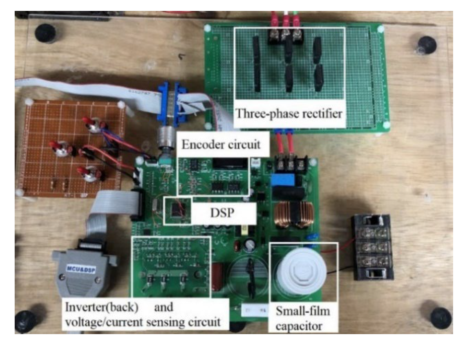
Figure 8 shows a photograph of the hardware circuits in this proposed drive system, including a three-phase rectifier, an encoder circuit, a DSP which is used to execute the high-frequency high-order active damping control, the predictive speed-loop control, and the predictive current-loop control, a six-IGBT inverter in the back of the PCB, voltage sensing circuits, current sensing circuits, and a small-film capacitor which has a much smaller size than traditional electrolytic capacitors. A comparison of the volume, weight, and cost of a traditional electrolytic capacitor and a small-film capacitor is shown in

Table 1. Comparison of different capacitors.

Types	Electrolytic Capacitor	Small-Film Capacitor
Characteristics
Volume	$470 \mathsf{\mu }\mathrm{F}$	$10 \mathsf{\mu }\mathrm{F}$
Weight	41 g	35 g
Cost	USD $10	USD $4
Medium	Aluminium oxide	Metallized Film
Dielectric coefficient	8–8.5	2.2 ± 0.2
Polarity	Yes	No
Voltage Stress	450 V	1000 V
Life	Capacitor deteriorates within five years of use	Capacitor does not deteriorate

[20]. This small-film capacitor uses Metal Injection Molding (MIM) technology [21], and it can be used for low-speed, middle-speed, and high-speed motor drive systems.

6. Simulated and Experimental Results

A 10 $\mathsf{\mu }\mathrm{F}$ small-film capacitor is used here, and the DC-bus voltage varies from 270 V to 311 V with a frequency of 360 Hz. Furthermore, a three-phase 220 $V_{rms}$ 60 Hz AC source is used. A 4-pole IPMSM with a rated power of 500 W, a rated current of 3 A, and a rated speed of 1800 r/min is also used. This motor has the following parameters: the stator resistance is 1.9 $\Omega$, the d-axis inductance is 15.1 mH, the q-axis inductance is 31 mH, the flux linkage is 0.227 V.s/rad, the inertia of the motor is 0.0005 kg.m${}^2$, and the viscous coefficient of the motor is 0.003 N.m.s/rad. This simulation uses Simulink software, and the $i_q{}^{max}$ is 2.5 A and the $i_q{}^{min}$ is 0.2 A. In order to verify the correctness of the theoretical analysis, several simulated and measured results are shown and compared, which can be divided into three categories. The first category includes the input AC source voltages, the input AC source currents, and the DC-link voltages using a 440 $\mathsf{\mu }\mathrm{F}$ electrolytic capacitor and a 10 $\mathsf{\mu }\mathrm{F}$ small-film capacitor. The second category includes the measured current waveforms using a predictive current controller and a PI controller. The third category includes the measured speed responses with and without constraints, including transient responses, load disturbance responses, and sinusoidal tracking and triangular tracking responses.

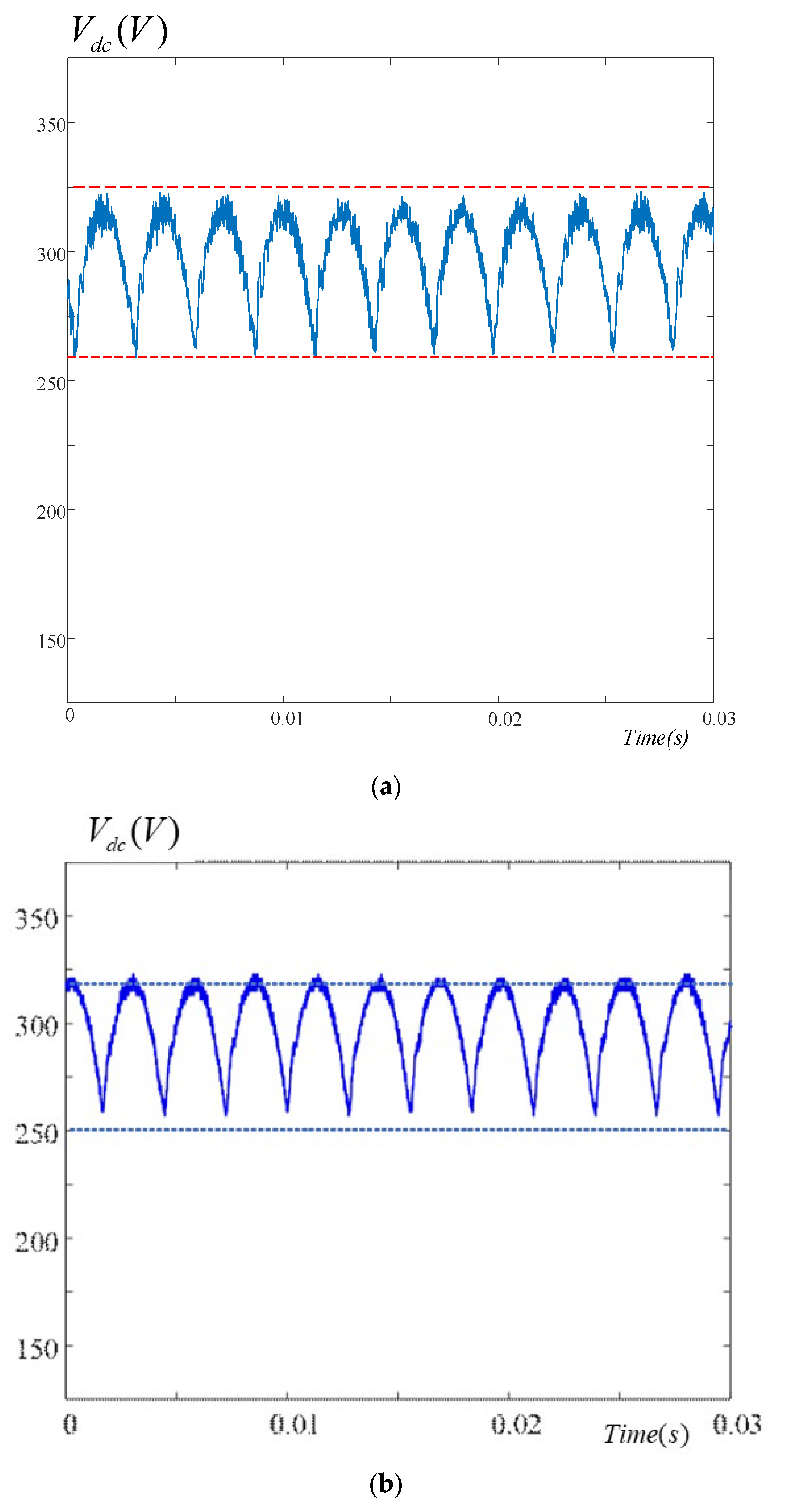
The measured results of the first category are demonstrated in Figure 9a,b, Figure 10, Figure 11, Figure 12a,b. Figure 9a demonstrates the simulated DC-link voltages using a small-film capacitor. The simulated DC-link voltages vary from 258 V to 320 V within a 2.76 ms. Figure 9b demonstrates the measured results using the same process. If we compare Figure 9a,b, we see that both of them have the same voltage and period fluctuations. We can see that the DC-bus voltage creates more serious fluctuations than traditional electrolytic capacitors. Figure 10a illustrates the simulated input currents at the AC source. The input current has a 3.5 A peak when using a 440 $\mathsf{\mu }\mathrm{F}$ electrolytic capacitor. Figure 10b illustrates the measured results by using the same process. After comparing Figure 10a,b, we can see that both of them have the same peak current fluctuations and also have the same two discontinuous current pulsations in each half cycle. The major reason for this is that when the input voltage is smaller than the DC-bus voltage, the rectifying diodes are turned off, and then the a-phase current becomes zero. 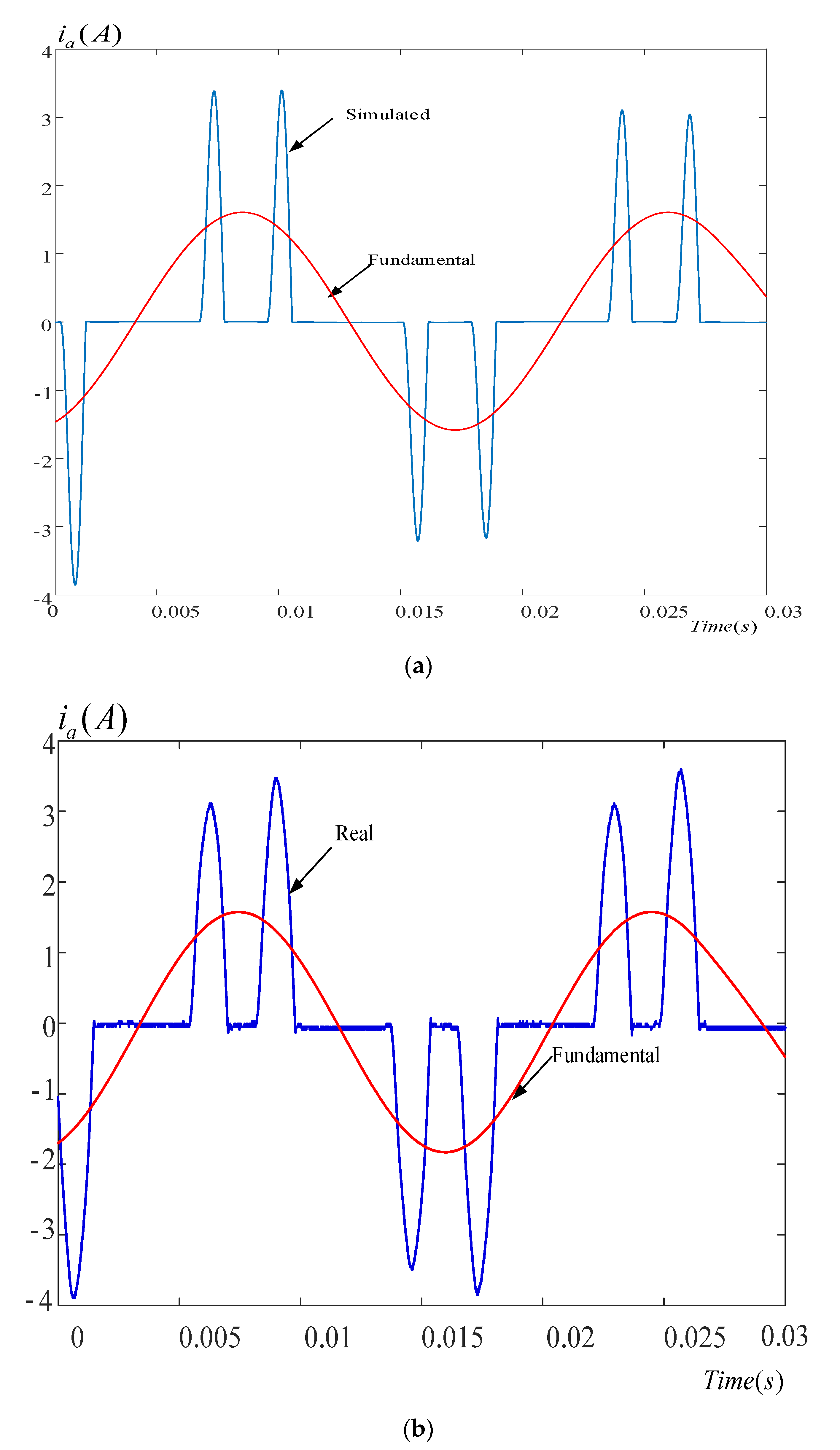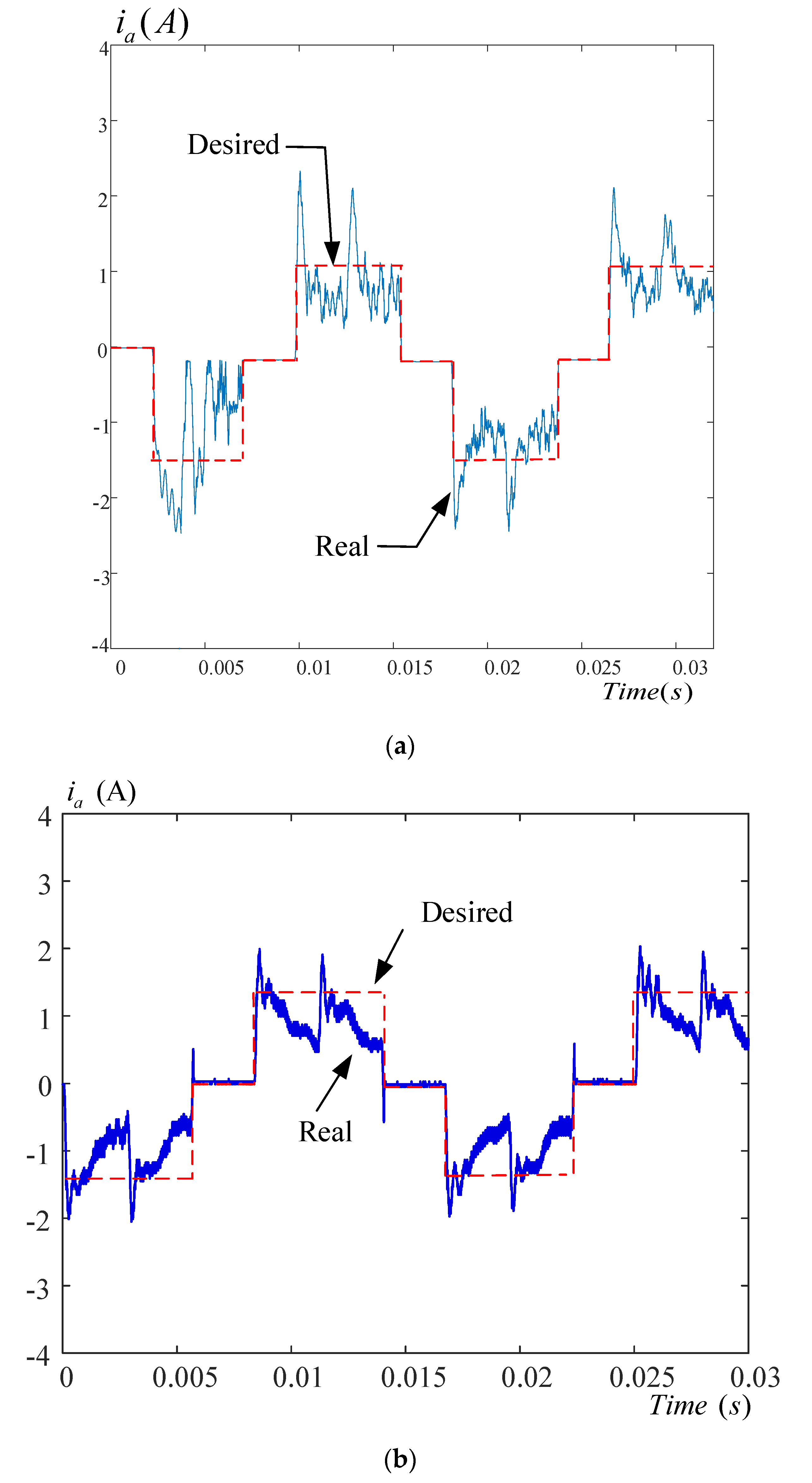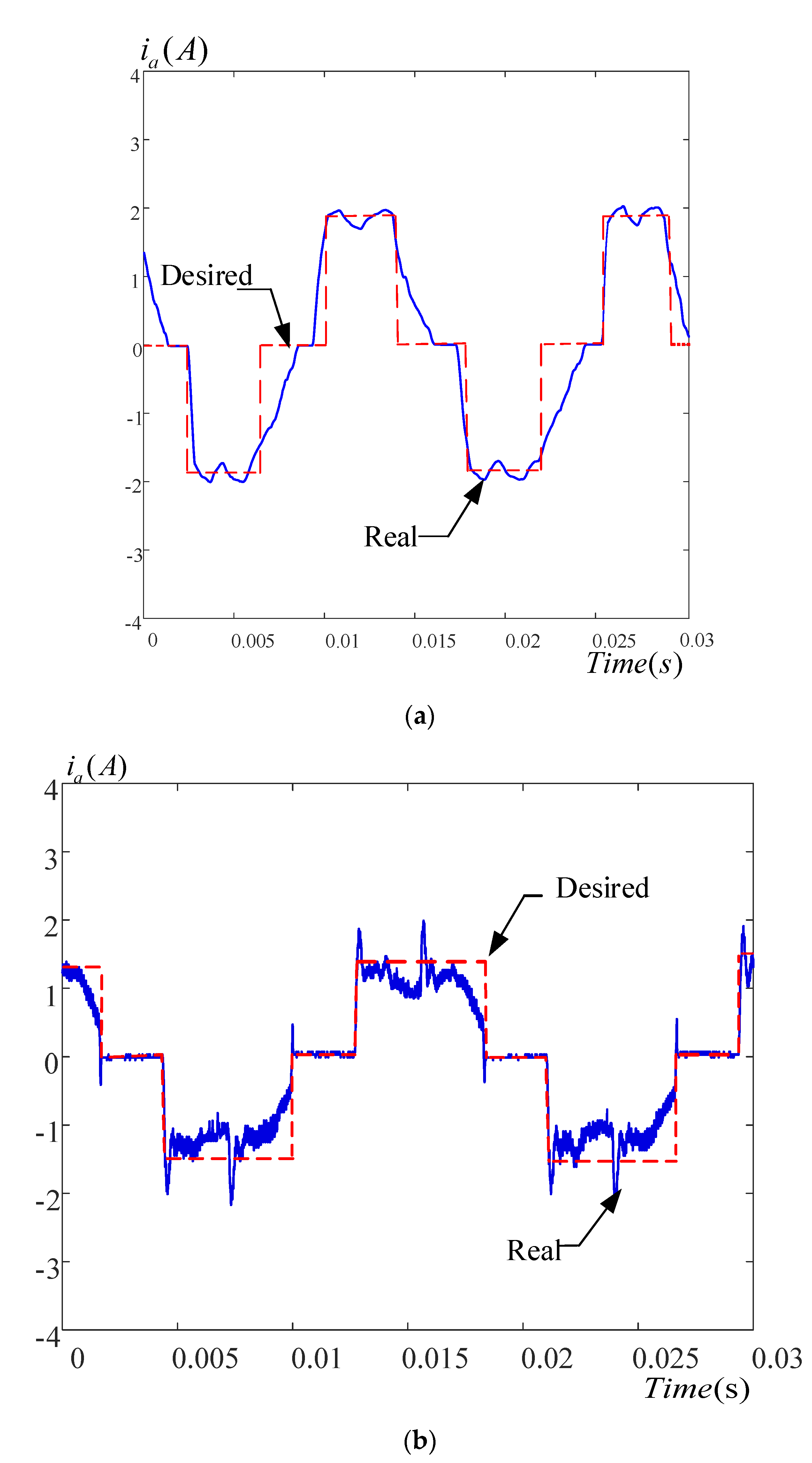Figure 11a shows the simulated input a-phase current at the AC source by using a 10 $\mathsf{\mu }\mathrm{F}$ small-film capacitor without using active damping control. Here, we can see that the input current has obvious pulsations. Figure 11b shows the measured waveform in the same situation. Both Figure 11a,b show that the desired square-wave currents are different from the measured currents due to their small inductance at the input AC source. When a small-film capacitor is used, the a-phase current changes from pulses into square waveforms because the DC-bus voltage is reduced. 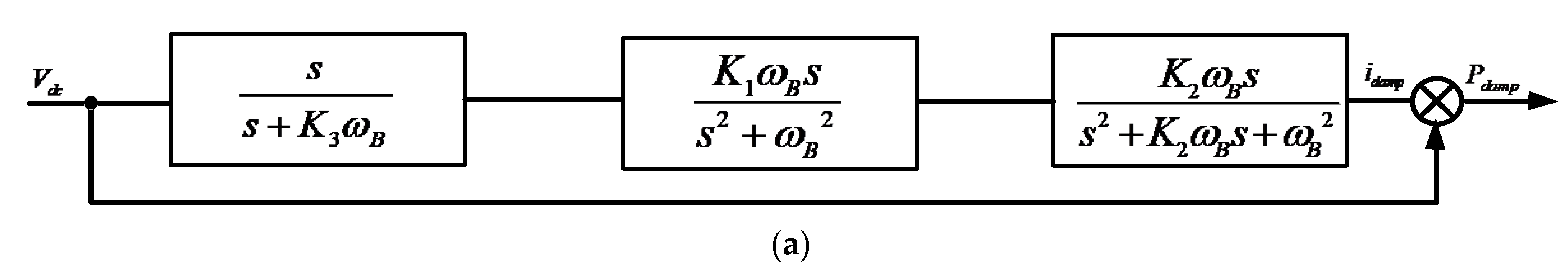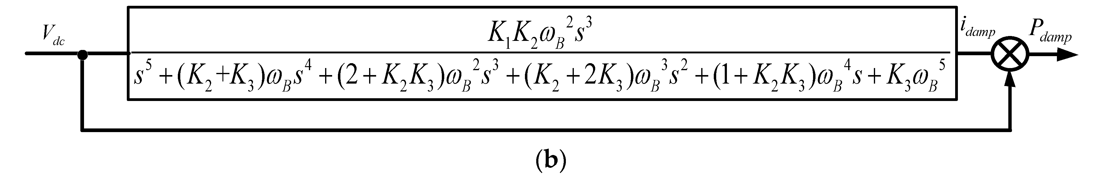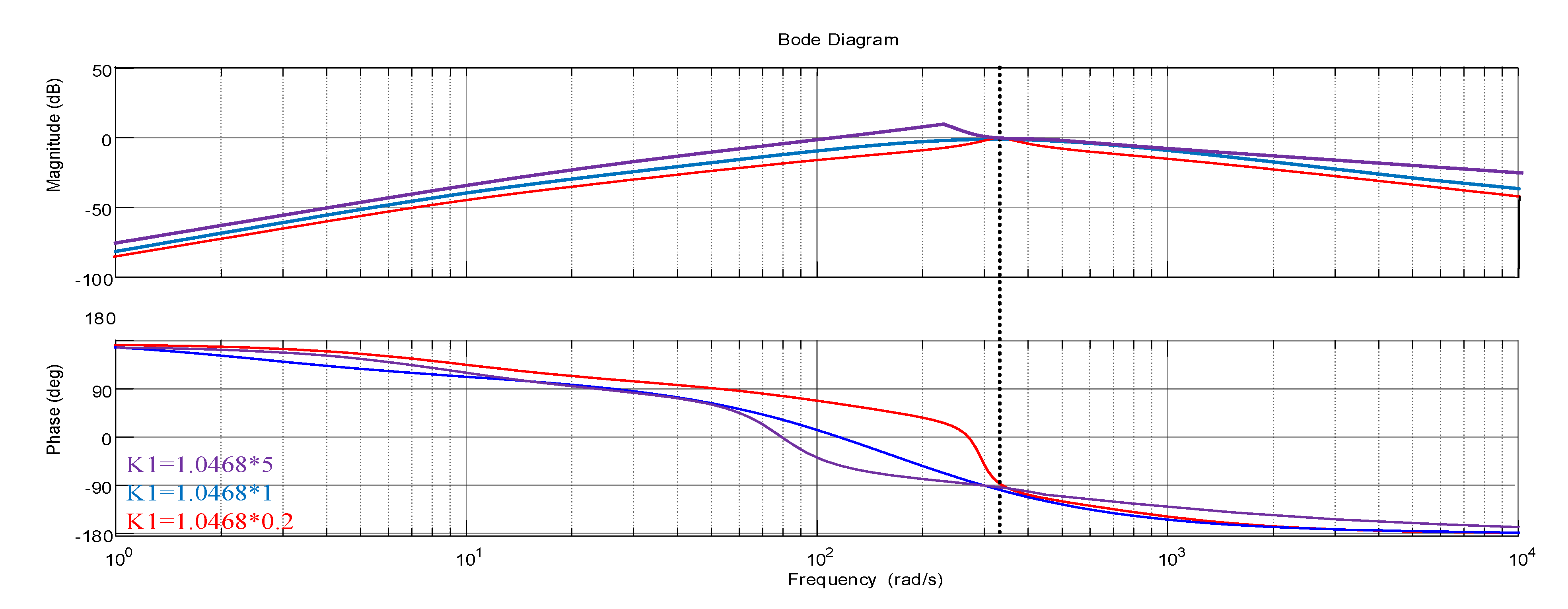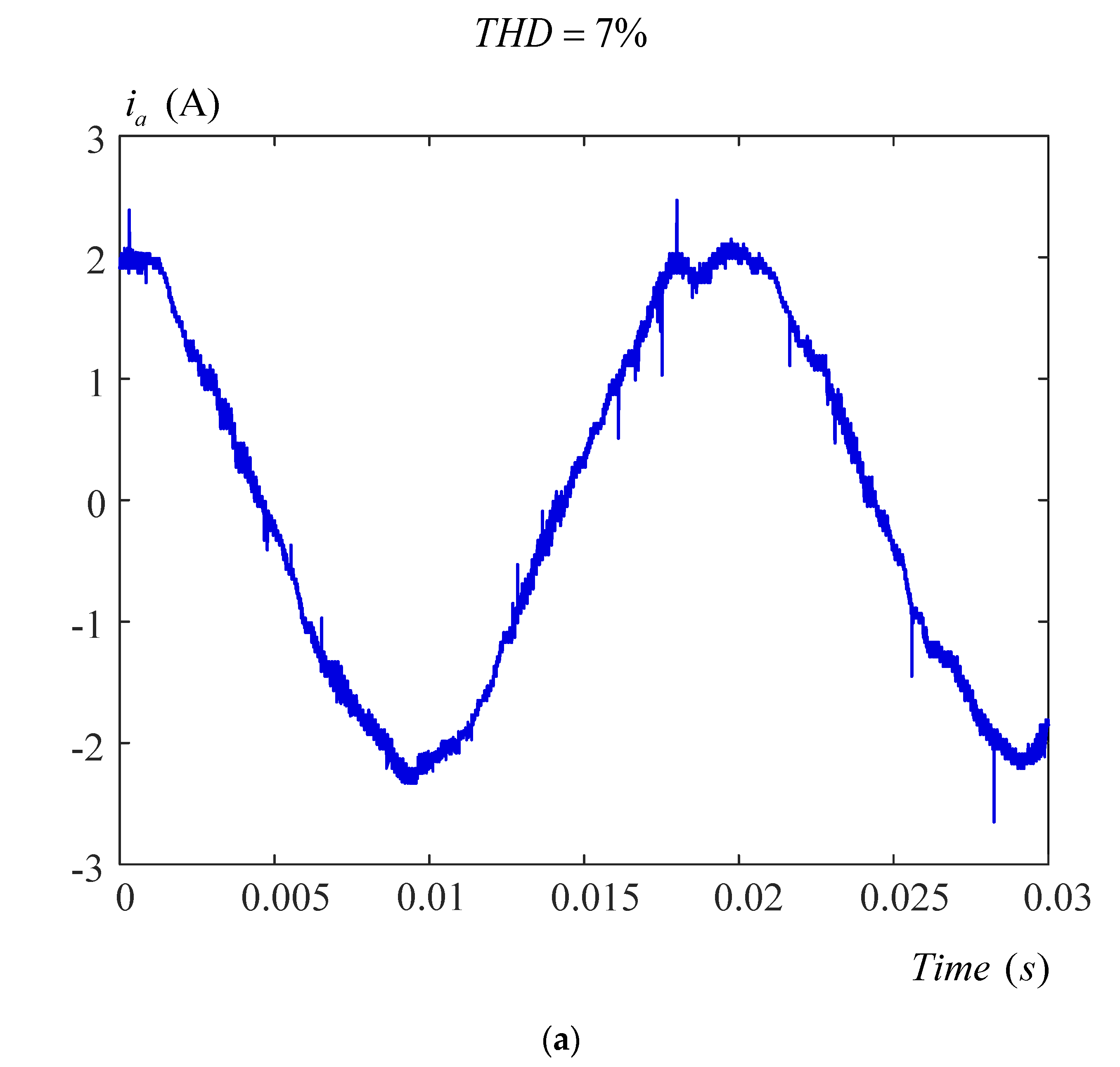Figure 12a displays the measured input current waveform using a high-order band-pass active damping control. The transfer function is $F(s)=\frac{K_1{K}_2{\omega }_B{}^2{s}^3}{s^5+(K_2+K_3){\omega }_B{s}^4+(2+K_2{K}_3){\omega }_B{}^2{s}^3+(K_2+2K_3){\omega }_B{}^3{s}^2+(1+K_2{K}_3){\omega }_B{}^{4}s+K_3{\omega }_B{}^5}$ with ${\omega }_B$ = 720$\mathsf{\pi }$ $\mathrm{rad}/\mathrm{s}$, K${}_1$ = 1.0468, K${}_2=$ 4.1095, and K${}_3$ = 0.00927. Figure 12b shows the measured input current using a first-order high-pass active damping control, which has a bandwidth of 5 kHz, and a cut off frequency of 2.26 kHz and can be expressed as $\frac{s}{s{+31400}_{}\mathrm{rad}/\mathrm{s}}$. As we can observe, the results in Figure 12a show a better performance than the results in Figure 12b. The major reason for this is that the fifth-order band-pass filter provides a wider middle-frequency bandwidth than the high-pass filter.

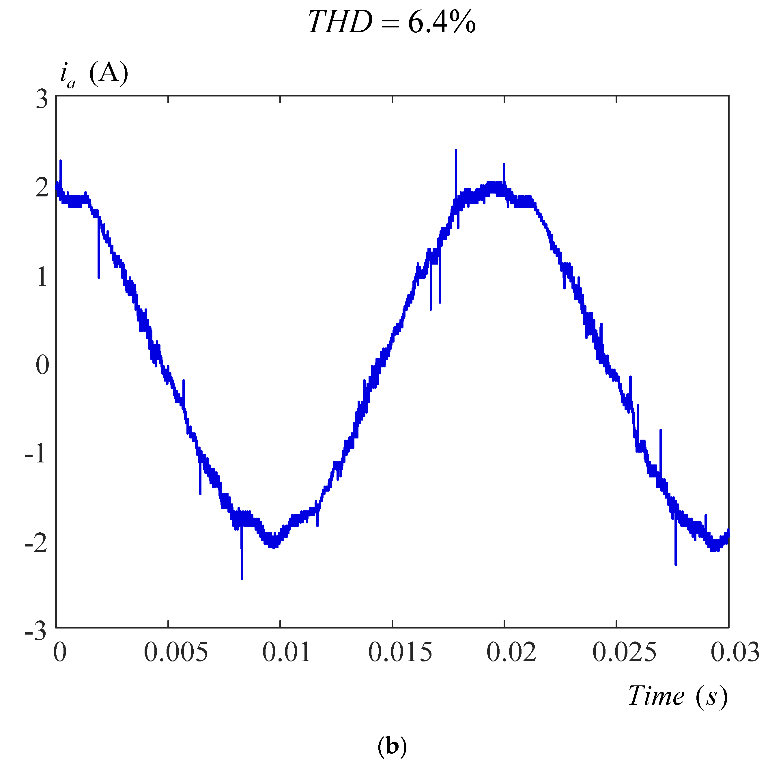
The measured results of the secondary category are demonstrated in Figure 13a,b. Figure 13a demonstrates the measured a-phase motor current by using PI current control, which generates a 7% THD. Figure 13b demonstrates the measured a-phase current by using predictive current control, which has a 6.4% THD. Again, the predictive current control provides better performance than the PI current control. The major reason for this is that the predictive control uses past, present, and future information to control the system; however, the PI control only uses present information to control the system.

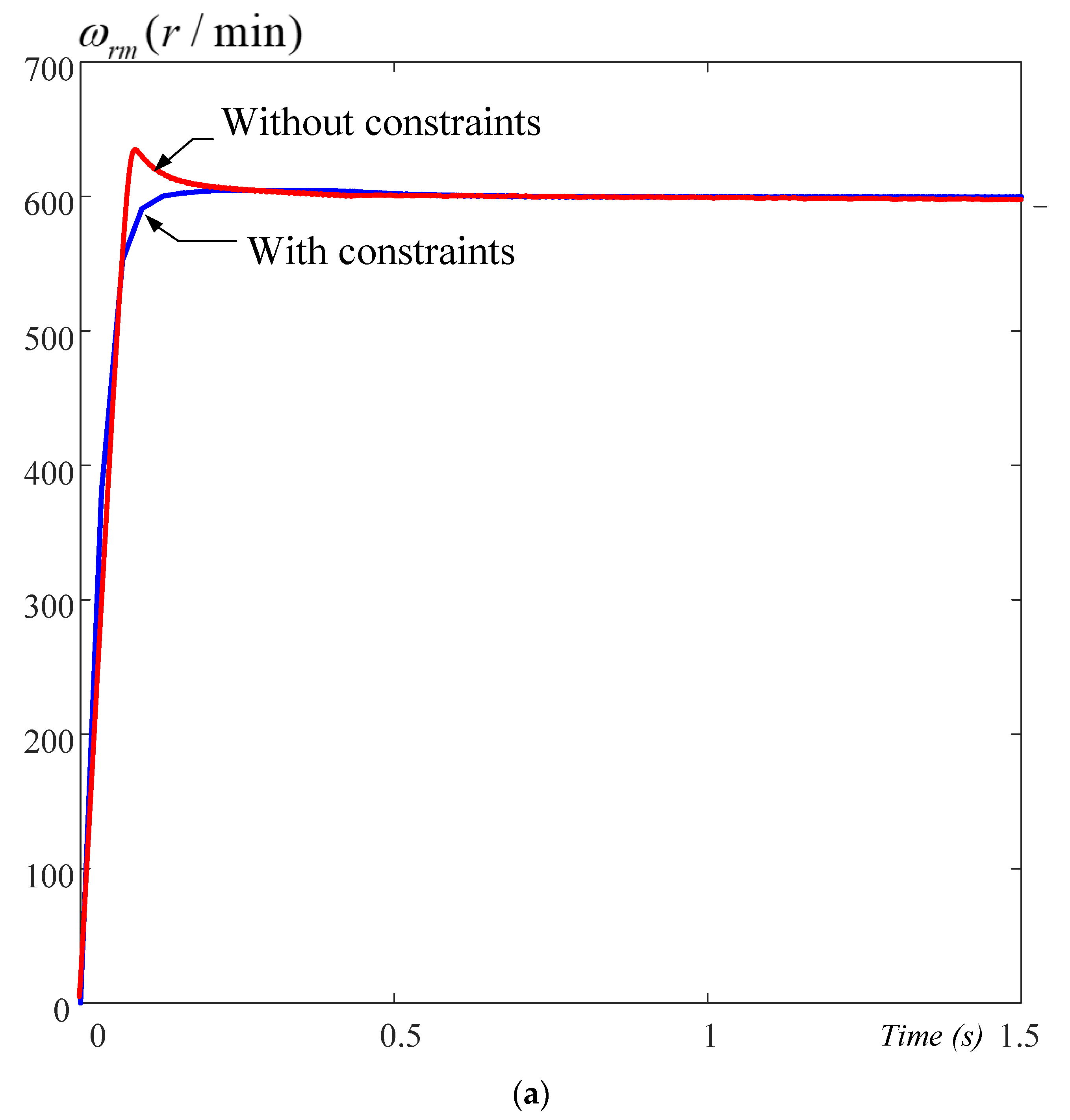
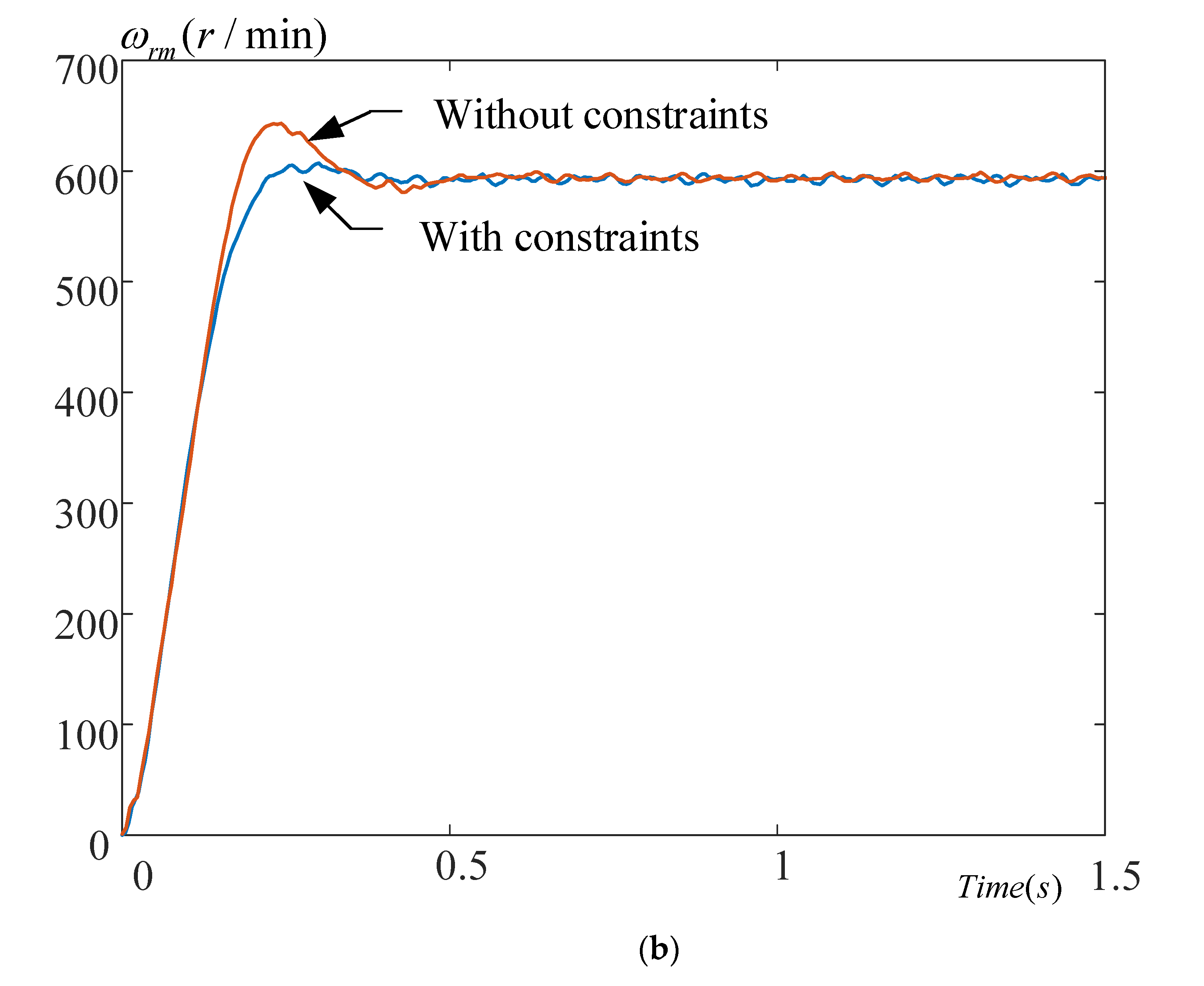
The simulated and measured results of the third category are shown in Figure 14a,b, Figure 15, Figure 16, Figure 17, Figure 18a,b. Figure 14a shows the simulated results of the predictive control with constraints and the predictive control without constraints. The predictive control with constraints has a lower overshoot than the predictive control without constraints. Figure 14b illustrates the measured results, which provide the same conclusions as the simulated results. 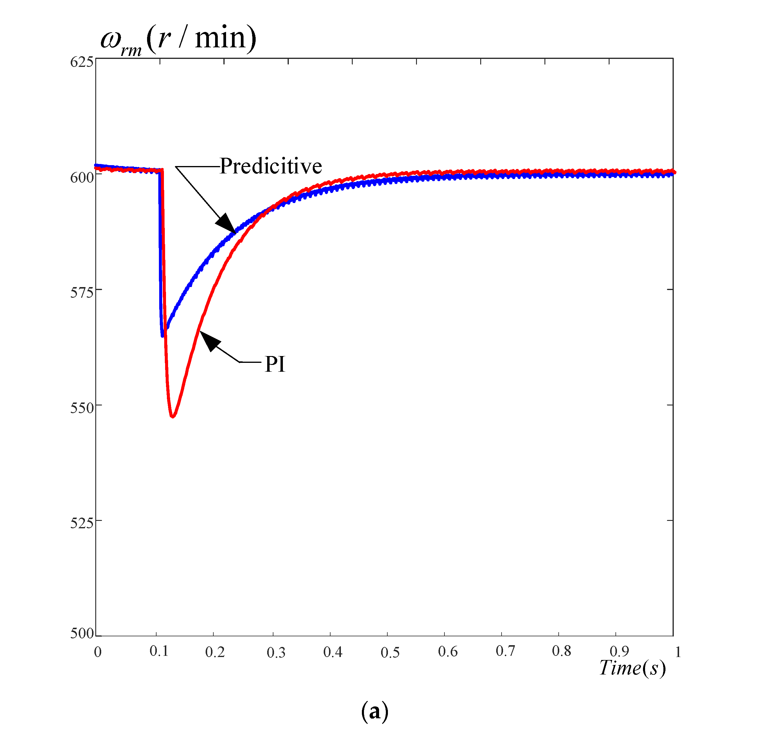Figure 15a shows the simulated results of the load disturbance with a 2 N.m external load. Figure 15b shows the measured results of the same situation. Both the simulated and measured results show that the predictive control provides a lower speed drop and a quicker recovery time than the PI control does. This is because the predictive control uses past, present, and future information to control the system. In addition, a real-time optimization of the cost function is applied. As a result, the predictive control shows better performance than the PI control. 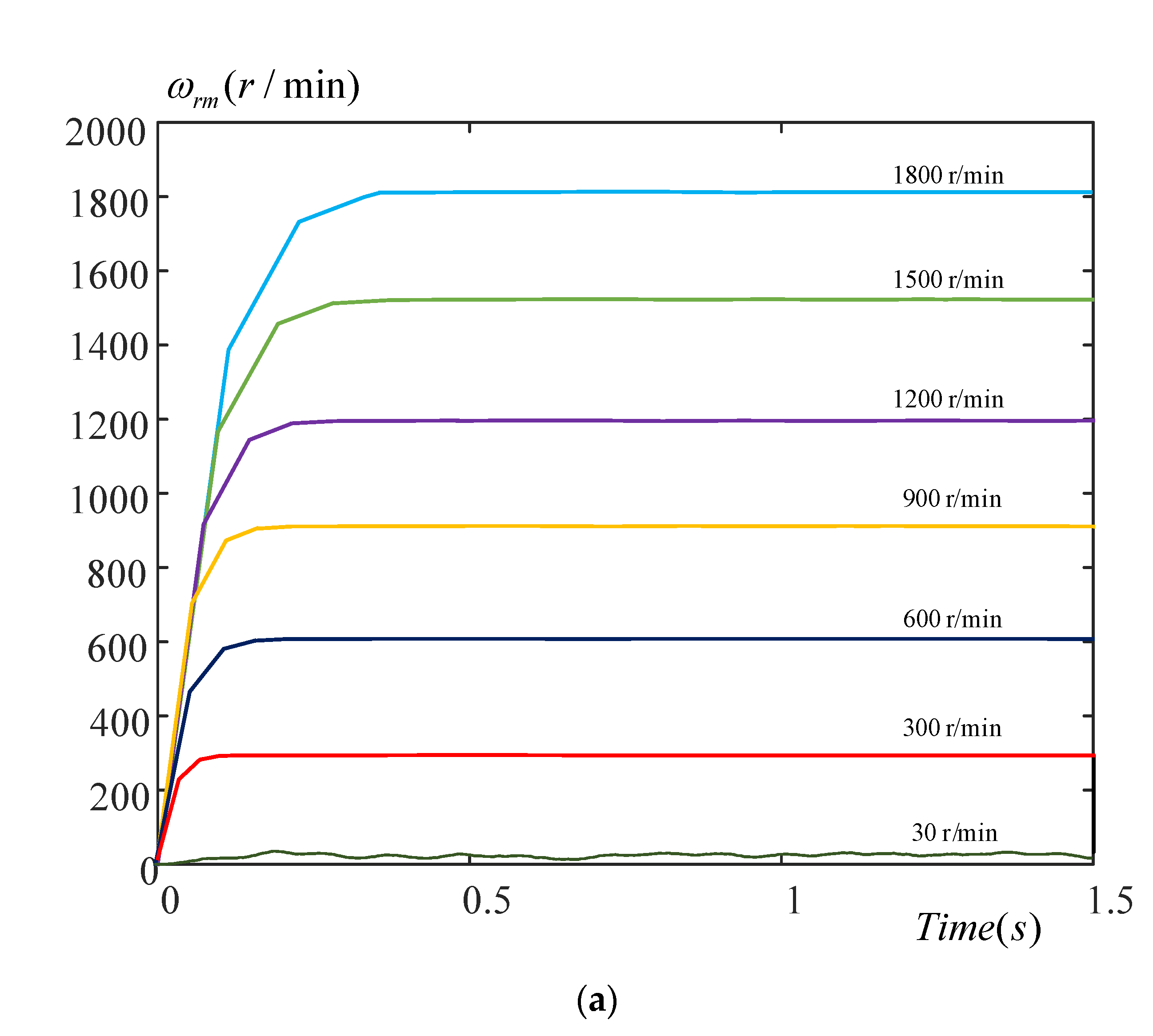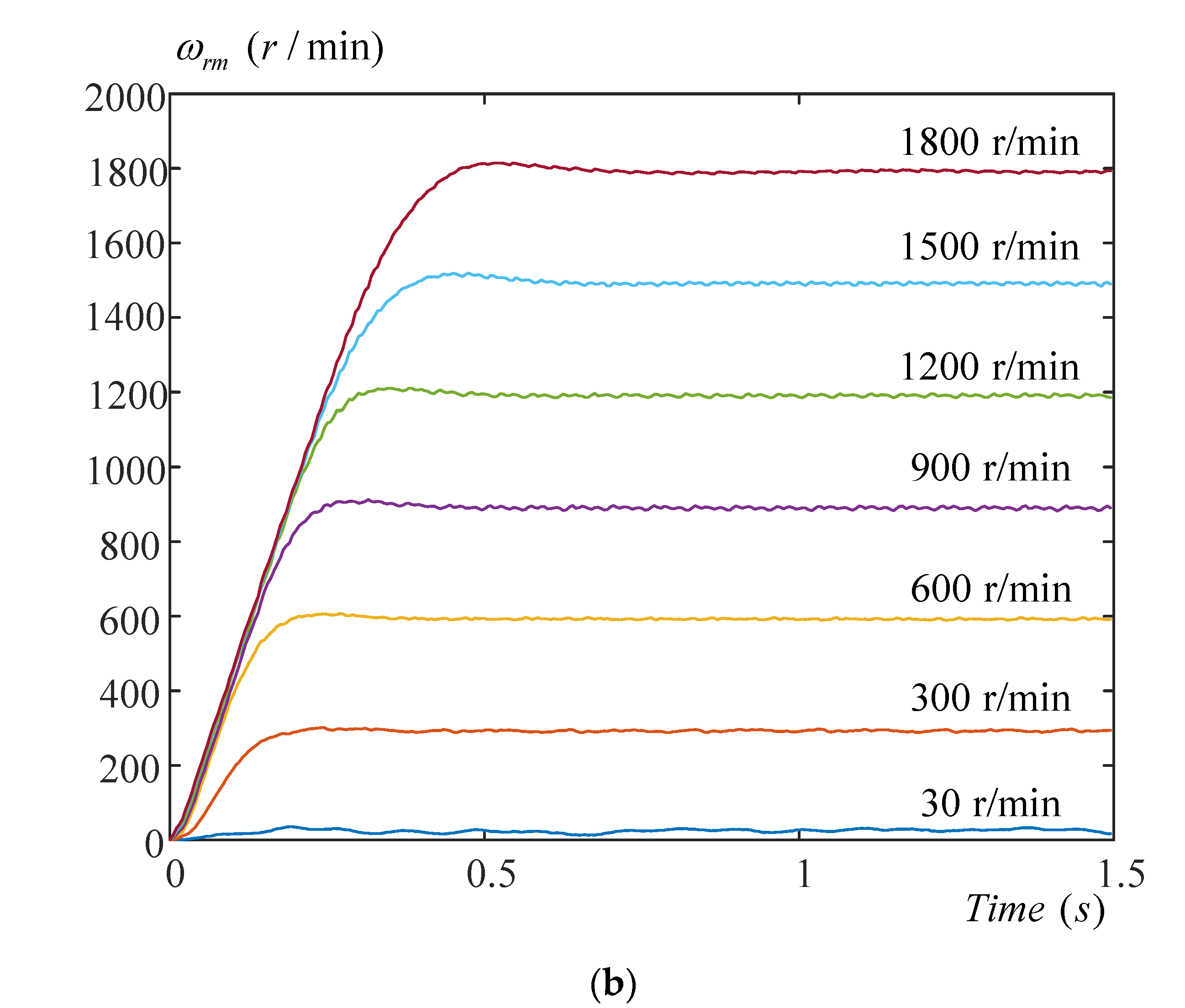Figure 16a shows the simulated speed responses from 30 r/min to 1800 r/min, and Figure 16b shows the actual measured responses. The results of simulated and measured responses are very similar. 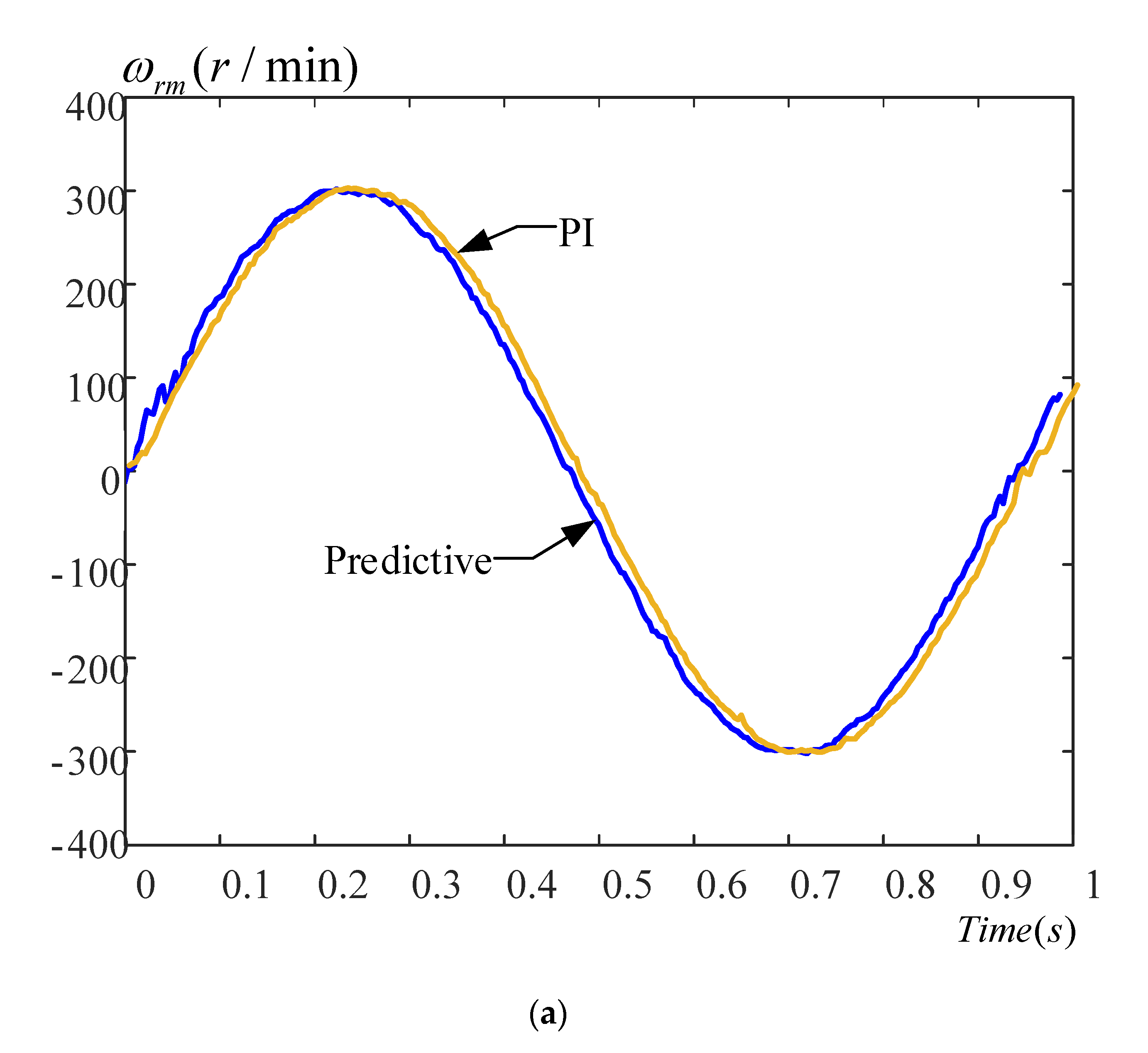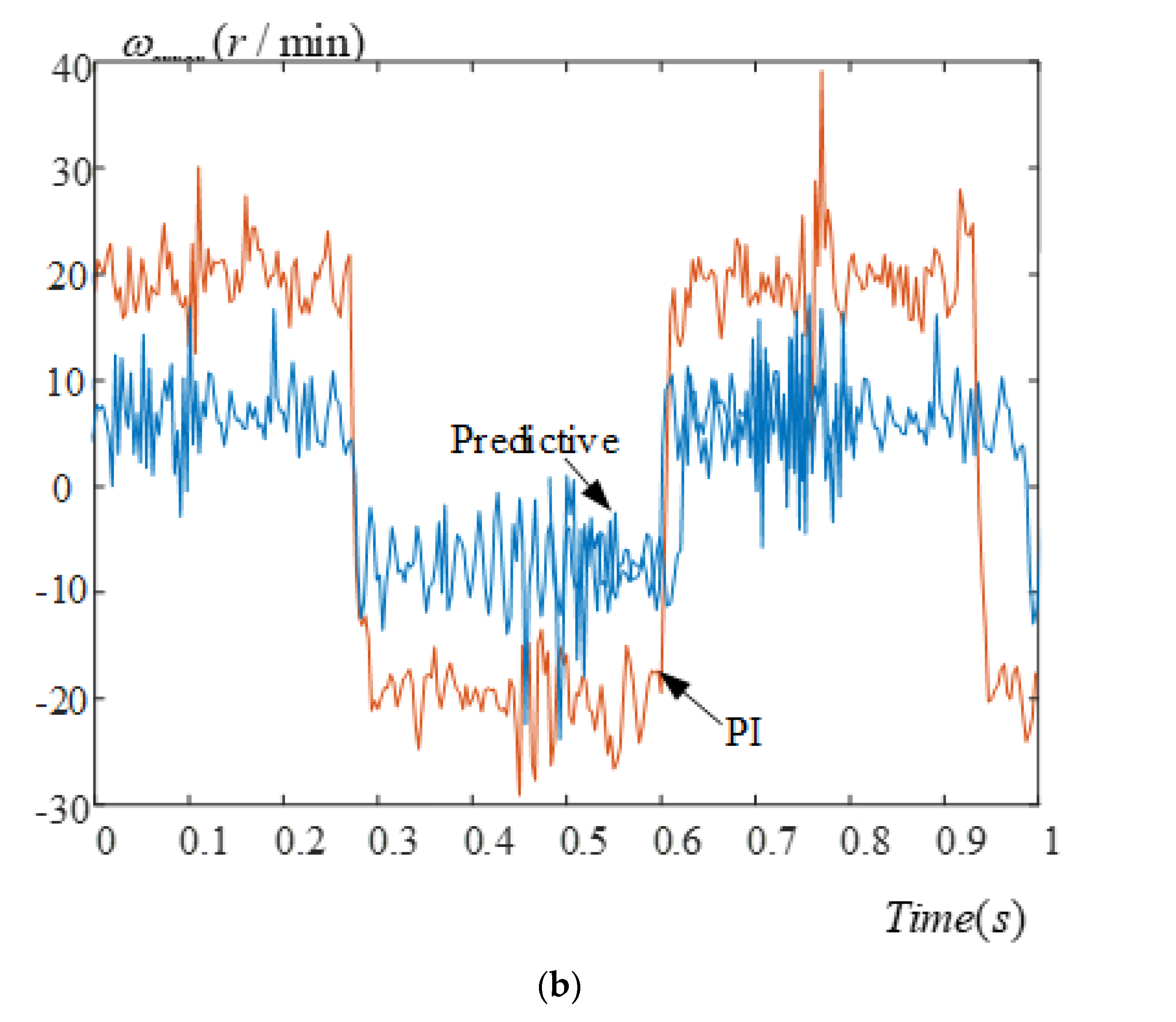Figure 17a shows the measured speed responses of a sinusoidal speed command at $\pm$300 r/min. We can see that the predictive control can follow the speed commands well, but the PI control has lagging responses. Figure 17b shows the speed errors, and we can see that the PI control has greater speed errors than the predictive control does. 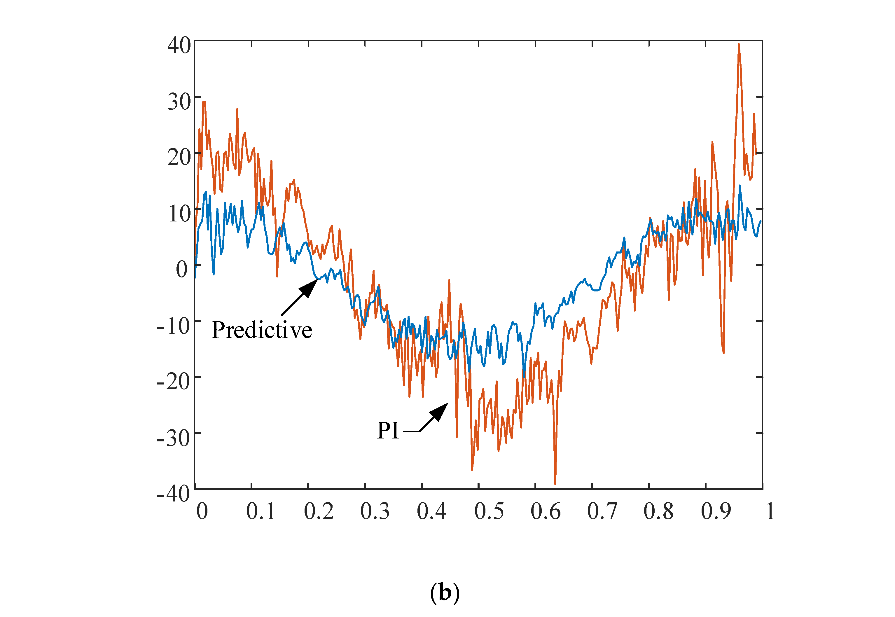Figure 18a displays the measured speed responses of a triangular speed command at $\pm$300 r/min, and we can observe that the predictive control has a better tracking ability than the PI control does. Figure 18b displays the speed tracking errors, and the predictive control provides $\pm$10 r/min tracking errors; however, the PI control has $\pm$20 r/min tracking errors. Thus, we can see that the predictive control has better performance than the PI control because the predictive control uses real-time optimization techniques. The PI control, however, uses integrational control, and this causes serious time delays. Generally speaking, in this paper, the speed errors in steady-state conditions are $\pm 2$ r/min, and the current errors in the steady-state conditions are $\pm 0.3$ Ampere. In addition, the THD of the a-phase, b-phase, and c-phase currents is near 6.5% when using the predictive control and active damping control.

7. Conclusions

In this paper, a high-order band-pass active damping controller is proposed to eliminate the input harmonic currents of small-film capacitor IPMSM drive systems. A systematic predictive constrained speed controller is designed to improve the transient, load disturbance, and tracking responses. Furthermore, a systematic predictive constrained current controller is used to reduce motor harmonic currents, in which a Lagrange multiplier is used to calculate the input constraints. After that, an optimization technique is employed to obtain the control input. A DSP, type TMS320F28035, manufactured by Texas Instruments, is used as a control center. Experimental results validate the theoretical analysis. Although the development of the predictive constrained control algorithms is complicated, the implementation of the predictive constrained control algorithms is very simple.

The proposed drive system in this paper has lower input harmonic currents and a better power factor than electrolytic capacitor DC-link inverters. In addition, this small-film DC-link capacitor drive system has a smaller size, a lower cost, and a longer life than traditional electrolytic capacitor DC-link IPMSM drive systems.

References

1. Inazuma, K.; Utsugi, H.; Ohishi, K.; Haga, H. High-power-factor single-phase diode rectifier driven by repetitively controlled IPM motor. IEEE Trans. Ind. Electron. 2013, 60, 4427–4437. [Google Scholar] [CrossRef]
2. Zhao, N.; Wang, G.; Xu, D.; Zhu, L.; Zhang, G.; Huo, J. Inverters power control based on DC-link voltage regulation for IPMSM drives without electrolytic capacitors. IEEE Trans. Power Electron. 2018, 33, 558–571. [Google Scholar] [CrossRef]
3. Bao, D.; Pan, X.; Wang, Y. A novel hybrid control method for single-phase-input variable frequency speed control system with a small DC-link capacitor. IEEE Trans. Power Electron. 2019, 34, 9016–9032. [Google Scholar] [CrossRef]
4. Son, Y.; Ha, J.I. Discontinuous grid current control of motor drive system with single-phase diode rectifier and small DC-link capacitor. IEEE Trans. Power Electron. 2017, 32, 1324–1334. [Google Scholar] [CrossRef]
5. Son, Y.; Ha, J.I. Direct power control of a three-phase inverter for grid input current shaping of a single-phase diode rectifier with a small DC-link capacitor. IEEE Trans. Power Electron. 2015, 30, 3794–3803. [Google Scholar] [CrossRef]
6. Li, H.; Wang, Q.Y.Q.; Luo, H.; Hou, Y. A novel DC-link voltage feedback active damping control method for IPMSM drives with small DC-link capacitors. IEEE Trans. Ind. Electron. 2022, 69, 2426–2436. [Google Scholar] [CrossRef]
7. Jung, J.; Lim, S.; Nam, K. A feedback linearizing control scheme for a PWM converter-inverter havin g a very small DC-link capacitor. IEEE Trans. Ind. Appl. 1999, 35, 1124–1131. [Google Scholar] [CrossRef]
8. Liutanakul, P.; Pierfederici, S.; Meibody-Tabar, F. Application of SMC with I/O feedback linearization to the control of the cascade controlled-rectifier/inverter-motor drive system with small DC-link capacitor. IEEE Trans. Power Electron. 2008, 23, 2489–2499. [Google Scholar] [CrossRef]
9. Mathe, L.; Torok, L.; Wang, D.; Sera, D. Resonance reduction for AC drives with small capacitance in the DC link. IEEE Trans. Ind. Appl. 2017, 53, 3814–3820. [Google Scholar] [CrossRef]
10. Wang, D.; Lu, K.; Rasmussen, P.O.; Mathe, L.; Feng, Y.; Blaabjerg, F. Voltage modulation using virtual positive impedance concept for active damping of small DC-link drive system. IEEE Trans. Power Electron. 2018, 33, 10611–10621. [Google Scholar] [CrossRef] [Green Version]
11. Khaled, N.; Pattel, B. Practical Design and Application of Model Predictive Control-MPC for MATLAB and Simulink Users; Elsevier: Oxford, UK, 2018. [Google Scholar]
12. Sitbon, E.; Ostrovsky, R.; Malka, D. Optimizations of thermo-optic phase shifter heaters using doped silicon heaters in rib waveguide structure. Photonics Nanostruct.-Fundam. Appl. 2022, 51, 101052. [Google Scholar] [CrossRef]
13. Moshaev, V.; Leibin, Y.; Malka, D. Optimizations of Si PIN diode phase-shifter for controlling MZM quarature bias point using SOI rib waveguide technology. Opt. Laser Technol. 2021, 138, 106844. [Google Scholar] [CrossRef]
14. Kwak, B.; Um, J.H.; Seok, J.K. Direct Active Reactive Control of Three-Phase Inverter for AC Motor Drives With Small DC-Link Capacitors Fed by Single-Phase Diode Rectifier. IEEE Trans. Ind. Appl. 2019, 55, 3842–3850. [Google Scholar] [CrossRef]
15. Velander, E.; Kruse, L.; Wiik, T.; Wiberg, A.; Colmenares, J.; Nee, H.P. An IGBT Turn-ON Concept Offering Low Losses Under Motor Drive dv/dt Constraints Based on Diode Current Adaption. IEEE Trans. Power Electron. 2018, 33, 1143–1153. [Google Scholar] [CrossRef]
16. Zhang, Y.; Yin, Z.; Gao, F.; Liu, J. Research on Anti-DC Bias and High-Order Harmonics of a Fifth-Order Flux Observer for IPMSM Sensorless Drive. IEEE Trans. Ind. Electron. 2022, 69, 3393–3406. [Google Scholar] [CrossRef]
17. Hatua, K.; Jain, A.K.; Banerjee, D.; Ranganathan, V.T. Active Damping of Output LC filter Resonance for Vector-Controlled VSI-Fed AC Motor Drives. IEEE Trans. Ind. Electron. 2012, 59, 334–342. [Google Scholar] [CrossRef]
18. Rodriguez, J.; Cortes, P. Predictive Control of Power Converters and Electrical Drives; John Wiley & Sons: Hoboken, NJ, USA, 2012. [Google Scholar]
19. Yin, L.; Zhao, Z.; Lu, T.; Yang, S.; Zou, G. An improved DC-link voltage fast control scheme for a PWM rectifier-inverter system. IEEE Trans. Ind. Appl. 2014, 50, 462–473. [Google Scholar] [CrossRef]
20. Hcyncn. Aluminum Electrolytic Capacitors vs. Flim Capacitors. 2018.
21. Chen, W.; McCarthy, K.G.; Mathewson, A.; Copuroglu, M.; Brien, S.O.; Winfield, R. High-Performance MIM Capacitors Using Novel PMNT Thin Films. IEEE Electron. Dev. Lett. 2010, 31, 996–998. [Google Scholar] [CrossRef]
Figure 1. Block diagram (a) main circuit, (b) damping control, (c) block diagram of damping control.
Energies 15 07449 g001aEnergies 15 07449 g001b
Figure 2. Block diagram of the proposed high-order bandpass filter to generate damping power. (a) cascaded form, (b) equivalent fifth order band-pass filter transfer function.
Energies 15 07449 g002aEnergies 15 07449 g002b
Figure 3. Bode diagram using different values of K 1 .
Energies 15 07449 g003
Figure 4. Relationship between the performance index and the constraint.
Energies 15 07449 g004
Figure 5. Flow-chart of the predictive speed-loop controller with constraints.
Energies 15 07449 g005
Figure 6. Flow-chart of the predictive d–q axis current control input voltage commands with constraints.
Energies 15 07449 g006
Figure 7. Implemented IPMSM drive system.
Energies 15 07449 g007
Figure 8. Photograph of the hardware circuits.
Energies 15 07449 g008
Figure 9. Measured dc-bus voltage using a 10 μ F small-film capacitor. (a) simulated, (b) measured.
Energies 15 07449 g009
Figure 10. Using 440 μ F electrolytic capacitor. (a) simulated, (b) measured.
Energies 15 07449 g010
Figure 11. Waveforms using the 10 μ F small-film capacitor without damping. (a) simulated AC input currents, (b) measured AC input currents.
Energies 15 07449 g011
Figure 12. Waveforms using the 10 μ F small-film capacitor damping control. (a) measured input currents using a high-order band-pass, (b) measured input current using a first- order high-pass.
Energies 15 07449 g012
Figure 13. Measured a-phase motor currents. (a) PI control, (b) predictive control.
Energies 15 07449 g013aEnergies 15 07449 g013b
Figure 14. Transient speed responses using different controllers. (a) simulated, (b) measured.
Energies 15 07449 g014aEnergies 15 07449 g014b
Figure 15. Load disturbance at 2 N.m. (a) simulated (b) measured.
Energies 15 07449 g015aEnergies 15 07449 g015b
Figure 16. Speed responses at different speed commands. (a) simulated, (b) measured.
Energies 15 07449 g016aEnergies 15 07449 g016b
Figure 17. Measured results of a sinusoidal speed command at ±300 r/min. (a) speed responses, (b) speed errors.
Energies 15 07449 g017aEnergies 15 07449 g017b
Figure 18. Measured results of a triangular command at ±300 r/min. (a) speed responses, (b) speed errors.
Energies 15 07449 g018aEnergies 15 07449 g018b