
Predictive Controller for Refrigeration Systems Aimed to Electrical Load Shifting and Energy Storage
by
 , , and
Edoardo Di Mattia
1, 
Agostino Gambarotta
2,3,
Emanuela Marzi
2,
Mirko Morini
1,2,3,* and
Costanza Saletti
2 1
Interdepartmental Research Center on Food Safety, Technology and Innovation (SITEIA.PARMA), University of Parma, Tecnopolo Padiglione 33, Campus Universitario, 43124 Parma, Italy
2
Department of Engineering and Architecture, University of Parma, Parco Area delle Scienze 181/A, 43124 Parma, Italy
3
Center for Energy and Environment (CIDEA), University of Parma, Parco Area delle Scienze 181/A, 43124 Parma, Italy
*
Author to whom correspondence should be addressed.
Energies 2022, 15(19), 7125; https://doi.org/10.3390/en15197125
Submission received: 4 August 2022
/
Revised: 21 September 2022
/
Accepted: 26 September 2022
/
Published: 28 September 2022
(This article belongs to the Topic Energy Saving and Energy Efficiency Technologies)
Abstract
:The need to reduce greenhouse gas emissions is leading to an increase in the use of renewable energy sources. Due to the aleatory nature of these sources, to prevent grid imbalances, smart management of the entire system is required. Industrial refrigeration systems represent a source of flexibility in this context: being large electricity consumers, they can allow large-load shifting by varying separator levels or storing surplus energy in the products and thus balancing renewable electricity production. The work aims to model and control an industrial refrigeration system used for freezing food by applying the Model Predictive Control technique. The controller was developed in Matlab® and implemented in a Model-in-the-Loop environment. Two control objectives are proposed: the first aims to minimize total energy consumption, while the second also focuses on utilizing the maximum amount of renewable energy. The results show that the innovative controller allows energy savings and better exploitation of the available renewable electricity, with a 4.5% increase in its use, compared to traditional control methods. Since the proposed software solution is rapidly applicable without the need to modify the plant with additional hardware, its uptake can contribute to grid stability and renewable energy exploitation.
1. Introduction
Refrigeration systems, used for freezing food, air conditioning, or industrial processes, play an important role in the field of energy. Indeed, the refrigeration sector is responsible for approximately 20% of the overall electrical energy used worldwide, and it is estimated to be responsible for 7.8% of global greenhouse gas (GHG) emissions. This sector will grow further over the next few decades, both due to the increasing cooling needs in several fields and global warming, and it is expected that the global electricity demand for refrigeration could more than double by 2050 [1].
Regarding the food industry, in this sector, refrigeration processes are essential, as they ensure the preservation of perishable foods. The annual report on frozen food consumption, carried out by the Italian Institute for Frozen Food (IIAS), states that in 2020, the consumption of frozen food by Italians grew by approximately 5.5% compared to its use in 2019 (with an average of 15.1 kg of frozen food per capita per year). This result shows how the COVID-19 pandemic has changed people’s behavior, but also highlights the importance of frozen foods as a means of sustenance, thanks to their long-term preservation [2]. Vapor compression refrigeration cycles (VCCs) are by far the most used technology for freezing food, even though research is being carried out on other technologies because of the need to find more sustainable solutions and improve the global efficiency of the systems [3].
In order to meet the objectives of the Paris Agreement and keep the global temperature increase below 2 °C compared to pre-industrial levels, a transition in global energy is needed, and this transition will be enabled by technological innovation, particularly in the field of renewable energy [4]. Nonetheless, when a high share of the energy market is covered by intermittent renewable energy sources, such as wind and solar, a flexible capacity to balance the difference between supply and demand over time and space is required. Flexibility services may be incorporated into the energy system through the use of storage technologies, flexible generation, or demand-side response schemes [5]. In this context, the study of new solutions and technologies that can offer these services and constitute a source of flexibility for the power grid is of great interest.
As previously mentioned, the refrigeration sector is responsible for a large amount of electricity consumption worldwide. Therefore, refrigeration systems draw great attention from researchers who aim to find solutions to optimize their performance in terms of energy and economic efficiency [6]. Their efficiency can be improved by optimizing the plant design, operating conditions, or technology used. Many optimization techniques have been developed and tested in this sector in order to achieve better system performance. Such optimization problems are highly non-linear and complex, and to solve them, many classical and non-classical approaches have been used in the literature [7].
Among the utilized strategies, predictive control has emerged in recent decades as one of the most successful control strategies for industrial applications [8]. Model Predictive Control (MPC) is a model-based optimization technique that uses a simplified model of the controlled system in order to predict its behavior. The controller calculates a sequence of control actions to apply to the system, which makes the future output of the system track a reference or minimize a cost function, over a time horizon, known as prediction horizon. Then, only the first control signal, corresponding to the first time-step, is effectively applied to the system, and the horizon rolls forward by one time-step. Afterward, the system states are measured or estimated, and they are given to the controller, which repeats the calculation for the new prediction horizon. This control method allows the real-time optimization of systems with multiple inputs and multiple outputs, as it uses current data on the actual behavior of the system for every calculation. When optimization also relies on the prediction of future disturbances, feed-forward MPC is obtained: The control action also takes into consideration such disturbances and the controller is able to anticipate their effects on the system. Due to the possibility of optimizing the system with respect to the forecast of future disturbances, and updating optimization constantly, MPC appears to be a suitable strategy to make refrigeration systems a source of flexibility for the grid and foster the integration of renewable sources.
In this paper, a controller based on the MPC technique for a vapor compression refrigeration system is developed and tested in a Model-in-the-Loop (MiL) platform. Two case studies were considered: in the first one, the aim of optimization is to minimize the total electrical energy consumed by the compressors, while the second case study considers the integration of renewable energy production and the goal is to minimize energy consumption while utilizing as much renewable electricity as possible and avoiding renewable energy curtailments or grid imbalances.
2. Literature Review
Given the necessity to reduce global GHG emissions and the fact that renewable energy sources still represent a low share of the market, the optimal operation of refrigeration systems is a key problem to be addressed [9]. In the review published by Bejarano et al. [9], many aspects of the modelling and global optimization of VCCs are investigated. The authors identify the three main factors involved, namely modelling, optimization, and control, and they analyze them in depth.
Among the existing control structures, Proportional-Integral-Derivative (PID) controllers are by far the most employed controllers in several industrial applications [10]. In 2018, Bejarano et al. [11] proposed a refrigeration benchmark (called Benchmark PID 2018) based on a general refrigeration cycle, with the aim to optimize the compressor speed and expansion valve opening in order to control the outlet temperature of the evaporator secondary fluid and the degree of superheating at the evaporator outlet. The benchmark also provided performance indices, which could be used for the comparison of different control strategies. The Benchmark PID 2018 was used in many studies, for instance, in [10], where the authors tested Han’s non-linear PID controller, or in [12], in which a tuning methodology to set the parameters of a multi-variable PID controller was proposed. In [13], the authors developed an Internal Model Control based on a PID controller and evaluated it with the Benchmark PID 2018, verifying its better performance compared to the benchmark system. In [14], a robust control applied to a refrigeration cycle problem was solved, using the active disturbance rejection approach through the design of General Integral Proportional observers and robust PID controllers, and the results were compared to the benchmark. Rodríguez et al. [15] proposed a different approach to the PID control design, which consisted of two decentralized PIDs, with one controlling the temperature of the evaporator secondary fluid and the other controlling the degree of superheating, by optimizing the compressor speed and the opening of the expansion valve. They applied two decentralized PID controllers to the system proposed by Benchmark PID 2018 and presented three different controller tunings. Other PID applications in refrigeration systems can be found in [16], where the authors compared the results of a linear and a non-linear formulation of the system, and in [17], in which an adaptive PID controller was applied to a system composed of solar photovoltaic air-conditioners, aiming to reduce the power gap between the air-conditioner load and the photovoltaic generation.
Conventional controllers, however, such as PID controllers, are closed-loop controllers that do not include a system model, and their performance is not ideal [18]. Instead, intelligent controllers or model-based control methods can achieve better performance [19]. Rasel et al. [7] formulated a detailed description of the key issues concerning the modelling and optimization of VCCs. They provided an exhaustive evaluation of the state-of-the-art approaches used for the modelling and optimization of refrigeration systems, which use computational intelligence techniques for their optimization. They highlighted the properties of the algorithms used, their computational efficiency, robustness, and applications. In addition, the authors discussed different surrogate modelling methods and their applications in the refrigeration sector. One of the most widely used computational intelligence techniques in the refrigeration sector is genetic algorithms, and they are well-known for global convergence [7]. Richardson et al. [20] presented a simulation tool with the potential for the design and optimization of steady-state vapor compression. They used genetic algorithms that allowed them to perform constrained optimization of a very large set of independent variables, including models of individual components. Zhao et al. [21] introduced a model-based optimization strategy for a vapor compression refrigeration cycle for the minimization of the total operating cost of energy consumed. They used a modified genetic algorithm together with a solution strategy for non-linear equations to obtain the optimal solution under different operating conditions. Zendehboudi et al. [22] investigated the behavior of R450A in refrigeration systems, and optimized the operation of the system, analyzing two different scenarios. A multi-objective optimization genetic algorithm is used, with the goal of reaching the maximum performance of the system. In [23], three scenarios were considered: thermodynamic optimization, economic optimization, and a multi-objective optimization problem, which considered both objectives simultaneously. The Pareto frontier was found by using a genetic algorithm. The results showed that the multi-objective design satisfies the thermodynamic and economic criteria better than two single-objective designs. Moreover, in [24], the authors tackled a multi-objective optimization problem using three different refrigerants, and a genetic algorithm was employed for the optimization. Finally, in [25], the optimization problem to achieve minimum total energy consumption was solved by using both particle swarm optimization and a genetic algorithm.
Other optimization methods based on artificial intelligence were applied to many studies to optimize these kinds of systems. For instance, artificial neural networks were employed to control multiple variables in a refrigeration system together with fuzzy control in [26], for performance and design process improvement in [27], and to predict the energy performance of the system and compare different refrigerants in [28].
Among the model-based approaches to optimization, Model Predictive Control is considered the largest recent achievement in the control literature, and it has been widely accepted as the next generation of practical control technology [19].
In their work, Dangui et al. [29] presented a practical method for tuning the parameters of an MPC algorithm, in order to optimize the suction and discharge pressures of the refrigerant compressor. Their study is proposed in a general way, giving the possibility to use it as a guideline for tuning an MPC controller for a refrigeration system. Yin et al. [30] developed a novel control strategy based on the MPC method to control the temperature of the evaporator of a vapor compression refrigeration system. Luchini et al. [31] designed a global linear MPC with the aim to achieve the desired cooling capacity for a long prediction horizon, and a mixed-integer MPC that provides the actual cooling capacity utilizing a short prediction horizon. A hierarchical MPC is obtained, and it enables the global linear MPC to utilize a long prediction horizon at low computational costs, while the mixed-integer MPC provides multi-objective optimization of the required cooling capacity. Yin et al. [32] proposed a novel optimization method based on self-optimizing control, for the selection of the optimal individual controlled variables for a VCC. MPC method-based controllers and PID controllers are then designed for the different set of control variables in order to optimize system operation. Hovgaard et al. [33] developed a non-linear MPC for the economic optimization of a supermarket refrigeration system, using the thermal storage capabilities of the system. The authors employed the refrigeration system’s flexibility to offer an ancillary demand response to the power grid and perform regulating services. They also took into consideration the uncertainties in both models and forecasts in their formulation. Non-linear predictive control was also proposed in [34,35], where the authors demonstrated the applicability and effectiveness of the method applied to a refrigeration system. Yin et al. proposed a cascade control [36]: depending on the cooling requirements of the user, in the outer loop, a PI controller provided the optimal setting values to be used in the inner loop, where an MPC controller was implemented with the aim to maximize system energy efficiency. Yang et al. [37] showed the results of the application of MPC to a VCC in the presence of known transient heat disturbances. The results showed an increase in the robustness of the system with respect to transient disturbances since the system could effectively prepare for them.
With reference to the status of scientific research, several studies were found that aimed at the optimization and control of refrigeration systems. Nevertheless, a lack of studies was found that investigate the possibility of using industrial refrigeration systems as a source of flexibility for the power grid, by shifting the electrical load and storing surplus renewable electricity in the frozen product. The novelties of this paper consist of:
- A novel predictive controller based on a Dynamic Programming algorithm, which decides the best control action at every time-step, in order to minimize the implemented cost function.
- The development of an optimization strategy with the goal to investigate the possibility to save energy by varying the level of refrigerant in the separators of a vapor compression refrigeration system.
- The analysis of the possibility to store surplus renewable energy in the frozen product in the form of thermal energy and make the refrigeration systems a way of adding flexibility to the power grid.
3. Digital Twin
The digital twin of the system, namely the mathematical model that reproduces the real system dynamics and its interaction with the environment, is necessary for MiL applications to test the control strategy if a real system is not available. In this section, the refrigeration system considered in this work is presented, and a brief description of the approach used for modelling the different components is given.
3.1. System Description
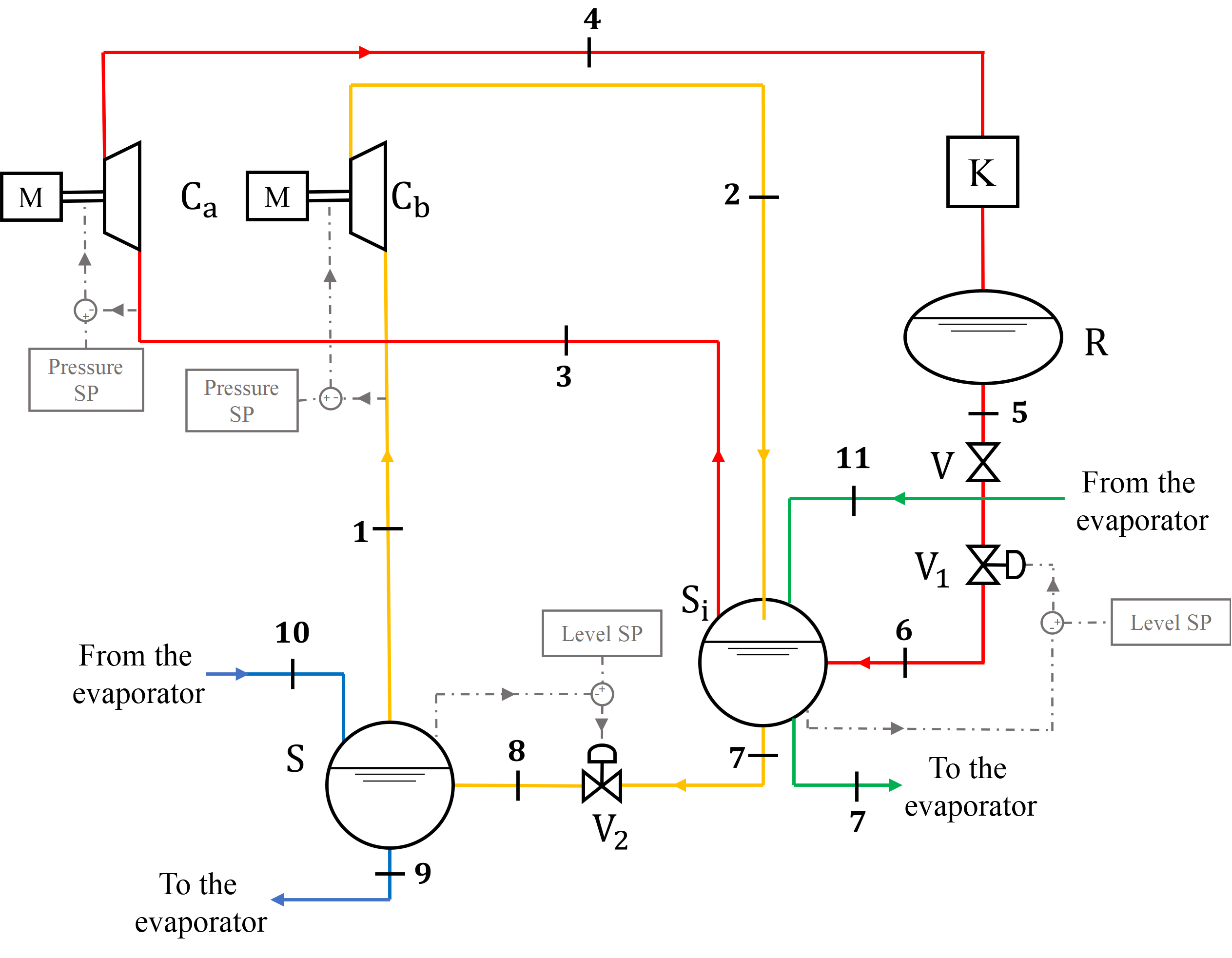
The system considered consists of an industrial refrigeration system, and it is represented in Figure 1. Ammonia is the working fluid, and three pressure levels are employed: Evaporation, intermediate, and condensation pressures. It is worth noting that the compression and expansion phases are divided into two steps, thanks to the adoption of the separators, and this provides the possibility to reduce the compression power, better operate the compressor, which works only with vapor, and exploit all latent heat of vaporization in the evaporation section [38].
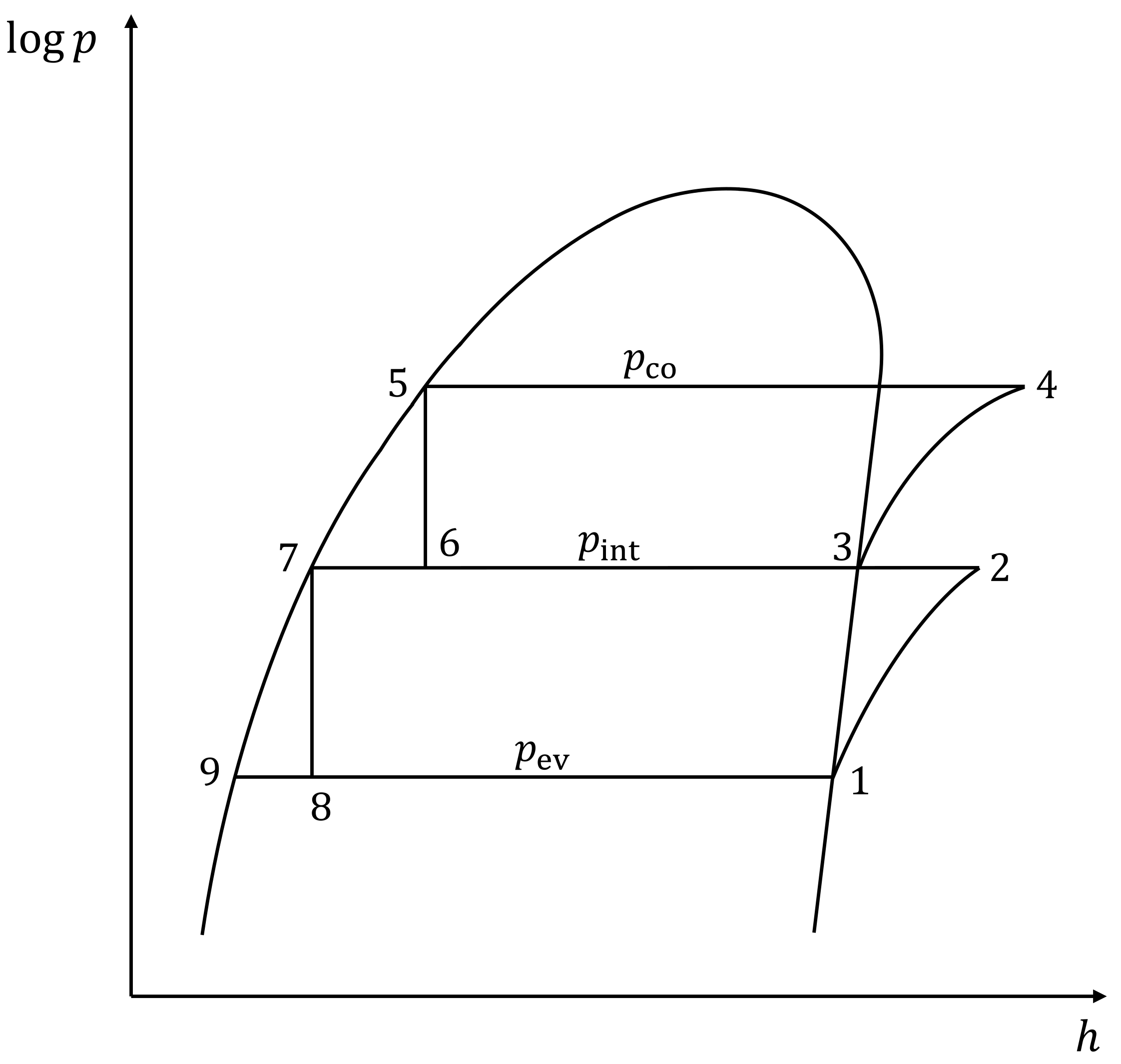
As schematized in Figure 1, the cycle operated by the working fluid is as follows: Starting from thermodynamic state 1, where it is at the vapor phase at evaporation pressure pev, the fluid is sucked by compressor Cb from low-pressure separator S, compressed until intermediate pressure pint, and discharged in intermediate separator Si (state 2). From this separator, a mass flow rate of gas is sucked by high-pressure compressor Ca (state 3) where the gas experiences compression until it reaches condensation pressure pco (state 4). The compressors are driven by electric motors M. After that, the compressed gas enters condenser K where it releases heat into the external environment through the phenomenon of condensation. The working fluid exits the condenser and reaches liquid receiver R, which balances the variations in the level of the separators. Subsequently, the fluid in the liquid phase (state 5) passes through expansion valve V1 and reduces its pressure from condensation pressure to intermediate pressure, entering separator Si (state 6). Here, the liquid ammonia (state 7) can evaporate (state 11) to produce, for example, cold water for food processing or can proceed through expansion valve V2, where it reduces its pressure until evaporation pressure (state 8) and enters separator S. Finally, the fluid enters the evaporation section (state 9) where it experiences a heat exchange with the air through evaporation (state 10), and returns to the separator, in the vapor phase, through the risers. The air is then employed for the food-freezing process. Therefore, by increasing the air flow rate in the refrigeration tunnel by controlling the fan rotational speed, the heat exchanged in the evaporator rapidly increases, as well as the ammonia mass flow rate. Then, a higher air flow rate means a higher heat exchange with the food. This leads to two possible effects: either the food reaches lower temperatures (when the refrigeration time is kept constant), or the amount of frozen food production increases (when the refrigeration time is reduced). On the other hand, a reduction in the heat exchanged in the evaporator cannot be achieved at the expense of an increase in food temperature, but through a reduction in the production rate. In Figure 2, all the thermodynamic states reached by the working fluid during the cycle are shown on the pressure-enthalpy diagram.
The main system components, as represented in Figure 1, are the screw-compressors, separators, the receiver, expansion valves, and the condenser. In the following sections, all the components of the plant are presented, and their operating principle is described, as well as how they were modelled.
3.2. Twin-Screw Compressor Model
A thermodynamic model of the twin-screw compressor was developed in Matlab® 9.7 R2019b. It is based on a set of non-linear algebraic equations that describes all the phenomena that occur during the compression process, including the leakages and heat transfers between the working fluid and compressor body. This model is a semi-empirical model and, as such, it requires the availability of the compressor performance map in order to identify some thermodynamic and geometrical parameters. The implementation of the model with its equations and the identification procedure was explained in detail in [39]. The key parameters of the twin-screw compressor model are suction mass flow rate and compression power . They are calculated as follows:
where n is the compressor rotational speed, is the swept volume (a geometrical parameter of the model), is the gas-specific volume at thermodynamic point 3, is the input compression power without losses, and and are the power losses due to internal load and viscous friction, respectively.
3.3. Separator and Receiver Models
The separators were modelled as drum boilers because of their operation [40]. They are dynamic components and were modelled through a set of differential equations for the conservation of mass and energy in the whole system and in the risers. It is a three-order model with three state variables: pressure p, liquid volume Vl, and average vapor quality at the riser outlet xr. The governing equations are:
where coefficients derive from the rearrangement of the balance equations and contain the geometrical properties of the separator and the thermodynamic properties of the fluid [40] and are reported in Appendix A.
The outputs of the model are the operating pressure and separator liquid level L. The latter can be calculated through the following equation:
where is the riser volume, is the area of the separator, and is a function of that represents the average vapor-liquid volume ratio in the risers [40].
Receiver R was modelled as was performed for the separators, but the equations presented above were rewritten because of the absence of risers and downcomers.
3.4. Expansion Valve Model
The expansion valve was modelled with an algebraic model described by a single equation for the mass flow rate [41]:
where is the orifice area and X is the pressure ratio:
Coefficient is the valve flow coefficient, and it was calculated through the following equation [42]:
where considers the pressure ratio, the valve opening ratio, and the presence of a biphasic fluid during the expansion, while coefficients are determined empirically.
Moreover, coefficient Y represents the expansion factor calculated through the following expression [43]:
where is the ratio between the specific heat ratio of a gas and the specific heat ratio of air, while represents the critical pressure ratio, which is a function of liquid pressure recovery factor , a feature of a specific valve that varies with the valve opening ratio.
3.5. Condenser Model
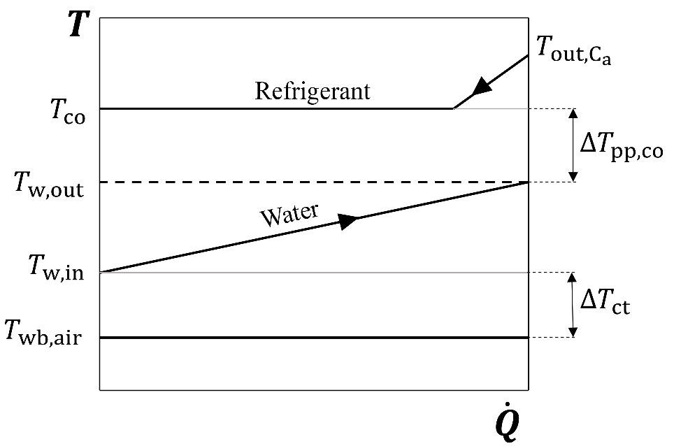
The condensation section is composed of a water-refrigerant fluid heat exchanger and a wet cooling tower to refresh the water. Therefore, it was modelled considering firstly the evaporative cooling of the water and then the heat exchanged to condensate the working fluid of the plant. Figure 3 shows the heat exchange diagram between the refrigerant fluid and water. Starting from the air dry-bulb temperature, relative humidity, and pressure, it is possible to calculate the air wet-bulb temperature . The water inlet temperature in the condenser is calculated as follows:
where is a temperature difference characteristic of the cooling tower (i.e., the cooling tower approach). In the condenser, water receives thermal power from the refrigerant and increases its temperature as follows:
where is the water mass flow rate and is the water specific heat. In real conditions, the condenser works with a pinch-point temperature difference , so the condensation temperature can be calculated as:
Finally, the condensation pressure is the saturation pressure of the refrigerant at the condensation temperature.
It is significant to note that the condensation pressure varies during the simulation with the external air conditions (i.e., pressure, temperature, and humidity). In fact, condensation pressure depends on the external conditions through condensation temperature . Therefore, the external temperature affects the power needed for the compressors to ensure the refrigerant reaches the condensation pressure. For example, when the external temperature is higher, the condensation pressure is higher and the compressors must use more energy, while when the external temperature is lower, they consume less electricity.
4. Control Strategy
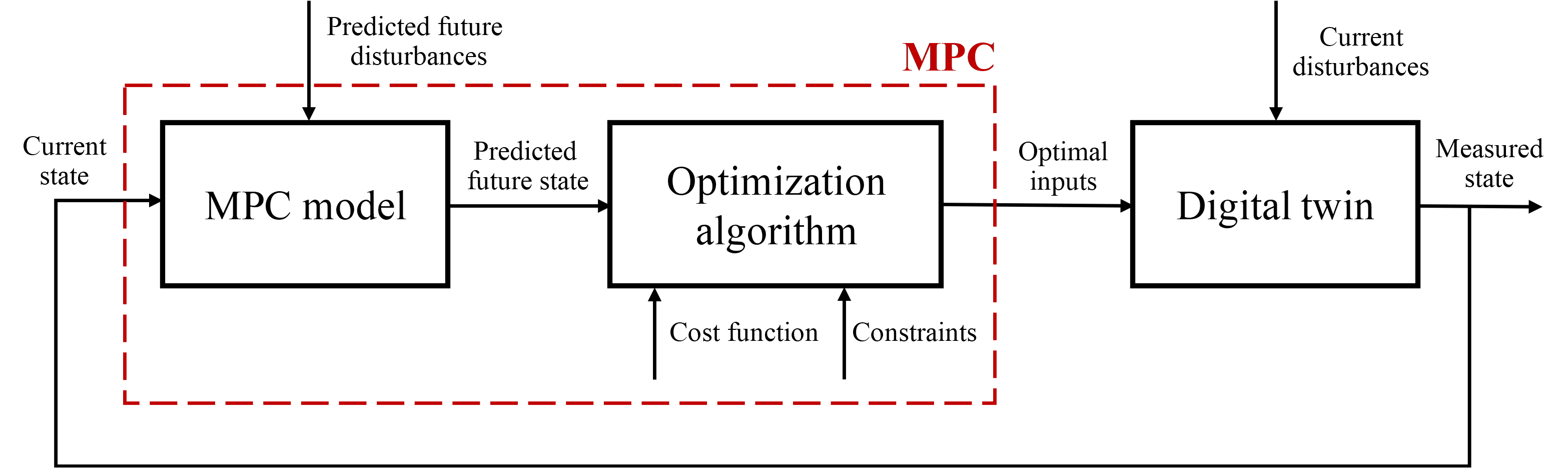
In this work, a smart controller based on MPC was developed and tested in a Model-in-the-Loop configuration. In Figure 4, the schematic representation of the controller application in the MiL is presented. As previously mentioned in Section 1 and represented in Figure 4, the developed predictive controller is composed of (i) a controller, (ii) a simplified dynamic model of the system to optimize, and (iii) an optimization algorithm that solves the optimization problem at each time-step and returns the optimal control actions.
4.1. The Optimization Algorithm
The Model Predictive Controller developed in this work relies on a Dynamic Programming algorithm, which is solved to find the optimal output and state, with the aim of minimizing a certain cost function. The optimization algorithm is based on the one developed in [44], in the case of a small-scale district heating system. Despite this specific application, however, the algorithm is highly versatile and can be extended to any energy-related case once the MPC simplified model is provided (see Section 4.2). Dynamic Programming is a numerical method based on Bellman’s principle of optimality [45], which states that the tail of an optimal trajectory for the problem variables calculated for the entire problem is still optimal when considering the tail subproblem. According to this theory, the time scale and the entire state-space of the optimization problem are discretized, and the optimization problem is divided into smaller subproblems, which are solved recursively going backward along the time scale. During this calculation, for each subproblem, the state function and the relative value of the cost function are evaluated for each admissible combination of the state and input grids. At each time-step, the inputs that minimize the cumulative cost for each eligible state are selected and memorized from the current step to the end of the forecast horizon. The procedure is repeated for the entire time horizon and allows the dynamics of the system to be included in the optimization. Therefore, this iterative computation returns an optimal control map for inputs and states, which is then used to identify the optimal control sequence through forward computation starting from the initial condition.
In this work, two control strategies were proposed and applied to the system. The cost function, as well as the inputs and disturbances of the controller, depends on the case study considered.
4.2. MPC Model
The predictive controller uses a simplified thermodynamic model of the system to simulate its behavior and calculate the optimal control sequence. It considers steady-state mass and energy balance for each component except for separator S, which is described by a single differential equation, which calculates the state, namely, separator level L:
with being the area of the separator, is the liquid density, and and are the mass flow rates of ammonia entering and exiting the separator, respectively.
Since the Dynamic Programming algorithm needs the discretization of the state and input grids, the model implemented in the MPC is obtained with the discretization of Equation (15). The discretized state equation at the k-th time-step, with a length of , is the following equation:
In the algorithm, the input and state grids are created according to their boundary values, while the steps of the grids are imposed according to the simulation algorithm parameters. The external disturbances given to the MPC are the forecasts of the environmental temperature and the power available from a photovoltaic plant integrated into the system.
At each time-step, the MPC calculates the control sequence to apply to the system, which minimizes the implemented cost function. Then, only the first element of the sequence is applied to the system. In particular, in the control strategies applied in this work, the two control actions considered are:
- The optimization of level L of the low-pressure separator, which is given as a setpoint to the PI controller that regulates the opening ratio of valve V2.
- The optimization of the heat exchanged in the evaporator with the frozen product, which is given directly as an input to the evaporator.
In real applications, the output signals of the controller are implemented with an inherent delay of a few seconds, due to the controller calculation time to perform the optimization. This delay in a MiL platform is usually neglected: the simulation time stops for the time interval needed by the controller to solve the optimization problem and starts again when the calculation is performed. To take this delay into consideration, it was set that the controller takes the state value corresponding to a time 30 s in advance, instead of taking the state value at the current time. The output, conversely, is implemented at the time-step. In this way, the signal delay due to the controller calculation time is simulated, and the simulation results obtained are closer to those corresponding to a real implementation.
5. Application
A MiL platform was used to test the innovative controller and compare it to a traditional control strategy: a system digital twin was built in order to emulate the real system, allowing the new control strategy to be tested as the real system was not available. The system was first modelled with a traditional control strategy, and then with the predictive controller described in Section 4, using the same external conditions. In this way, the two methods were compared, and the advantages of using a smart control technique were quantified. In this section, the implementation of the controller in the system model is presented, the case studies simulated are described, and some key performance indicators are identified, to evaluate the effectiveness of the control strategies applied.
5.1. System Digital Twin
As previously mentioned, the simulations are performed on a MiL platform. The controller was implemented in Matlab® and applied to the system digital twin, which was built by assembling the models of the single components presented in Section 3 in a coherent way in the Simulink® 10.0 environment. The set of equations is solved by a variable-step solver of the second order while thermodynamic properties of the fluids are evaluated through Coolprop [46]. The main parameters of the model are reported in Table 1.
As shown in Figure 1, several control chains are implemented in the system. They involve the control of the level in the two separators, by regulating the valve V1 and V2 opening ratio, and the control of the pressure in the separators, by regulating the rotational speed of compressors Ca and Cb. The implemented setpoints are constant for the entire simulation time span, except for the level setpoint of separator S, which is regulated by the MPC in the simulations in which it is applied to the system, as explained in Section 4.2. The setpoints used are reported in Table 2.
5.2. Description of the Case Studies
The considered system, represented in Figure 1, is an industrial refrigeration plant for freezing food. The predictive controller developed in this work was applied to the system, and two control actions were tested. In both case studies, the prediction horizon of the MPC, as well as the simulation time, is five days long.
Two disturbances are given to the predictive controller: the forecasts of the external temperature and the PV power production. These forecasts are different from the disturbances applied to the MiL; indeed, to simulate a real application, the real disturbances are obtained by applying small deviations to the ideal disturbances given to the controller. In this way, it is possible to evaluate how the predictive controller reacts with slightly different disturbances from those predicted, which is what usually happens in real applications.
In Figure 5, the trend of the forecast of the external temperature is shown: five summer days were simulated, during which the temperature ranged from 20 °C to 40 °C. The temperature presents a similar trend over the five days, with it being higher during the daytime and lower during nighttime.
The forecast of the second disturbance, namely the photovoltaic power, is displayed in Figure 6; over the five days, the system produces power during the day, with peaks of approximately 500 kW, while during the night, the production is nil.
As previously mentioned, two case studies were considered: they differ in terms of disturbances, the objective of the optimization, and controlled variables, and they are explained in the following sections.
5.2.1. Single-Objective Case Study: Minimization of Total Energy Consumption
In this case study, the electricity is considered entirely bought from the grid. The objective function of the control strategy is the minimization of the electricity consumed by the compressors, and it is mathematically expressed as follows:
with being the power used by the i-th compressor and the time-step length, i.e., 15 min. The MPC takes as input the actual mass flow rate at the V2 valve and, by using the separator level as a state and the external temperature as a disturbance, calculates the future control actions on the mass flow rate through the valve, and the future state. The state, namely separator level , is calculated using Equation (16). In this scenario, the evaporation heat exchanged with the air used to freeze the food product is taken as a constant and equal to = 400 kW.
5.2.2. Multi-Objective Case Study: Minimization of Total Energy Consumption and Exploitation of Renewable Energy Production
This case study considers the integration of photovoltaic energy generation in the system. The aim of the MPC is to optimize separator level L, by controlling mass flow rate at the valve, and thermal power exchanged in the evaporator. Unlike the previous case study, , and therefore the final temperature of the food product, is an optimization parameter here, and it is controlled by the MPC. The aim of the control is both to minimize the total energy consumption of the compressors and to minimize the difference between the energy produced by PV and the energy consumed by the compressor, when the latter is lower than the renewable energy production, with the goal to maximize the usage of the PV energy. The objective is the minimization of Equation (18)
where and are the weights associated with the two parts of the objective function, is the power employed by the i-th compressor, is the photovoltaic power produced, and is the time-step, which is 15 min, as in the previous case study.
To evaluate the benefits of the predictive controller compared to a traditional control strategy, different scenarios were simulated in this case study. The simulated scenarios are exposed in Table 3, and are the following:
- TC360, TC400, and TC440: in these three scenarios, a traditional control action is applied. In all scenarios, the low-pressure separator level setpoint is fixed at L = 1 m and they only differ in the value of the evaporation heat setpoint applied. These control strategies are useful to evaluate the results of the scenarios in which the MPC is implemented.
- MPC400: in this scenario, the MPC is applied; nevertheless, the evaporation heat is considered constant and equal to 400 kW, while the controller can only optimize low-pressure separator level L. The weights of the cost function are adequate to meet both objectives and they have been set after sensitivity analysis.
- MPC-ES: in this scenario, the MPC is applied, but only the first part of the cost function is considered, as and . Therefore, only the minimization of the total energy consumption is performed, and both level L and evaporation heat are optimized.
- MPC-ESRE: this scenario is the most complete. It considers both terms of the cost function, as in MPC400, with adequate weights, and both the evaporation heat and the low-pressure separator level are optimized, as in MPC-ES. Nevertheless, to estimate the benefits of this optimization, a comparison with the other considered scenarios is useful.
5.3. Key Performance Indicators
To evaluate and compare the results of the simulations considering a traditional control strategy and the innovative MPC method, three KPIs were selected:
- Total energy consumption (kWh): this is the amount of energy utilized by the system, which consists of the electrical energy used by the compressors.
- CO2 emissions (kg): this is the amount of carbon dioxide emitted, which is entirely related to electrical energy consumption. Indeed, the emissions associated with renewable energy generation are considered nil, while for electricity purchased from the grid, an emission factor equal to 0.4455 kgCO2/kWh is assumed [47].
- Renewable energy utilization (%): this is the percentage of renewable energy utilized by the compressors on the total energy produced by the photovoltaic system, only applicable to the multi-objective case study.
6. Results and Discussion
The system was simulated after modelling the overall refrigeration plant and the predictive controller in the Matlab®/Simulink® environment. The simulated scenarios were described in detail in Section 5.2, while the results of the simulations will be shown and explained in the following sections. The solutions obtained with the MPC strategies were compared to the results obtained with traditional control techniques, in order to highlight the benefits of the innovative controller.
The simulation time is five days in both cases. However, when dealing with the MPC, it optimizes the system only on the second, third, and fourth days. This was performed in order to compare the results of the two control strategies with the same initial and final state. Hence, the differences between the two simulations were collected over the three central days.
6.1. Results of the Single-Objective Case Study
The aim of the control here is to minimize the total energy consumption. The disturbance of the model is the external environmental temperature, the forecast of which is displayed in Figure 5, while the electricity is considered completely bought from the grid. The level setpoint calculated by the controller and implemented in the system is shown in Figure 7, where it is compared to the level setpoint implemented in the traditional control logic. It is possible to see how the innovative controller acts: while with the traditional control strategy the low-pressure separator level remains constant over the five days of simulation with a value of 1.00 m, in the new solution, the controller varies the low-pressure separator level between its lower bound (i.e., 0.50 m) and upper bound (i.e., 1.50 m). Therefore, the control logic decides to store liquid ammonia when the external environmental temperature presents low values and empty the separator when the external temperature is higher, and the compression of the ammonia is disadvantageous from an energy point of view. This type of control makes it possible to save energy and exploit it in a smarter way, as shown in Figure 8, where the power requested by the compressors in both solutions is compared. Important differences in the management of compressors can be noted. With the traditional controller, the energy used by the compressors is strictly related to the external temperature, and when it increases, the compressor power request also increases. Instead, with smart management, it is possible to consume more energy and store it in the separator level when it is advantageous from an energy point of view, and to reduce energy consumption when it is more expensive, i.e., when the external temperature is higher.
In Table 4, the values of the KPIs for these simulations are shown. They refer to the three central days of the simulations, namely the days on which the innovative control strategy is applied to the system. The energy saving results in 156 kWh for the three days, which is 0.69% of the total consumption. This means 52 kWh/day on average and, therefore, approximately 17 MWh/year of energy savings, considering that the plant operates for 330 days per year. In addition, 69 kg of carbon dioxide emissions is avoided over the three days, which implies 23 kg/day on average, i.e., 7590 kg/year.
These savings may seem of little significance if compared to the total consumption and emissions of the system, but it is relevant to highlight that it could be possible to achieve these results, when controlling a real refrigeration system, even without installing new hardware, but only by changing the setpoints of the existing controllers following the logic of the MPC.
6.2. Results of the Multi-Objective Case Study
In this scenario, the possibility of exploiting renewable energy was considered. In particular, the energy produced by a PV system was used to move the compressors and to store energy in frozen food. From a model point of view, the forecast of the power supplied by PV, displayed in Figure 6, was evaluated as a second disturbance in the MPC algorithm, in addition to the forecast of the external temperature, shown in Figure 5.
As in the previous case study, the control strategies are applied only on the three central days, while on the first and the fifth days, the level setpoint is fixed to 1 m and the evaporation heat is equal to 400 kW, also in the traditional control strategy scenarios.
Figure 9 shows the actual PV power production and the power used by the compressors with the different control strategies. As previously mentioned, the PV power production considered in the MiL presents small deviations from that used in the predictive controller (see Figure 6). These deviations were added to simulate a real environment, in which the forecast of a disturbance is different from the actual disturbance. In Figure 10, the low-pressure separator level management is shown, while in Figure 11, the evaporation heat management in the different scenarios is displayed.
Looking at the results of the simulations, it can be noticed that, on the three central days, the power consumption trend and the level management of the MPC-ES scenario are very similar to those obtained with the MPC control strategy in the single-objective case study: the objective in both cases is indeed the minimization of the total energy consumption. However, in the MPC-ES scenario, the possibility to vary the evaporation heat is added. During the three days, the control strategy acts by keeping the evaporation heat at its lower bound, i.e., 360 kW, in order to minimize consumption. Therefore, when looking at the power consumption, the MPC-ES trend follows the traditional control strategy TC360, and acts toward it as the MPC strategy acted toward the traditional control in the single-objective case study.
When analyzing the MPC400 scenario, which considers both terms in the cost function, it aims at the maximization of the renewable energy consumption during the day, while the energy saving strategy is postponed to the night. In fact, MPC400 presents lower power consumption during the night, when the renewable energy generation is nil, while it has higher consumption during the day, if compared to the traditional control strategy with the same evaporation heat value, namely TC400 (see Figure 11). The level setpoint is therefore increased in the evening, when there is still a little energy produced by the PV and the external temperature is low, in order to reduce the consumption at night, while in MPC-ES, the level decreases at the end of the day to save energy, since it is the period in which it is more expensive to operate the compressors.
Finally, the MPC-ESRE acts as MPC400, with the advantage of having the possibility to change the evaporation heat: when the PV power is higher than the compression power, in MPC-ESRE, the predictive controller manages the plant by increasing the heat exchanged in the evaporation section, in order to minimize the cost function and increase the share of renewable energy usage. In this scenario, the control decides to increase when surplus renewable electricity exists, decreasing the frozen food temperature, storing energy in the product, and allowing the system to act as a storage solution. In fact, when increases, the air speed in the refrigeration tunnel fans also increases, as well as the ammonia mass flow rate, which means that the food reaches a lower temperature for the same refrigeration time, with considerable advantages in its transport and storage. This scenario proves to be the most interesting from the point of view of the applied control strategy, as it includes both terms of the cost function, and it also optimizes the power exchanged in the evaporator.
In the current energy framework, which is moving toward renewable sources, this particular feature of refrigeration systems, representing an energy storage solution, is relevant. As it is well known, these sources, such as wind or solar, have an unpredictive nature, which can cause grid unbalances due to the difference between supply and demand. With smart control, as shown in this work, VCCs can be helpful in this context, as they can both store energy when needed in their separators and in the product, e.g., frozen food. As far as the authors are aware, this source of flexibility has not yet been adequately studied and it is therefore important to study its future potential. Furthermore, considering the integration of these systems into the power grid, ancillary services using this intelligent control could be offered. Indeed, when there is a surplus of energy in the electricity grid, refrigeration systems could provide balancing services.
It is interesting to compare the numerical results obtained with the traditional control strategy TC400 with those of the most complete scenario using the MPC control strategy, i.e., MPC-ESRE. As shown in Table 5, the management of the plant with the innovative controller applied in the MPC-ESRE scenario allows 4.5% more renewable energy to be exploited over the three central days than with the traditional control TC400. That means 758 kWh (with a minimum increase in energy requested by the compressors, equal to 104 kWh), i.e., 253 kWh/day and 83.4 MWh/year, considering that the plant operates 330 days per year. Furthermore, even though the total energy consumption of the MPC-ESRE control strategy is higher than the consumption of TC400, it performs better in terms of carbon dioxide emissions, since the plant utilizes a larger share of renewable energy, which is associated with nil emissions. The results show that with the MPC-ESRE there is a reduction in CO2 emissions of 291 kg over the three days compared to the TC400, which means 97 kg/day and 32 ton/year of avoided emissions.
7. Conclusions
Energy savings must be reached in many sectors in order to reduce greenhouse gas emissions and fight climate change, meeting the requirements imposed by the Paris Agreement. Refrigeration systems are responsible for a large amount of the total global energy consumption, and improvements in their optimal management need to be made.
Numerous studies have been performed in order to increase the efficiency of these systems and optimize their operation. Nevertheless, there is limited research into the possibility of using such systems as flexibility providers. Indeed, with the increasing share of renewable energy sources on the energy market, by using these systems as storage, sources of flexibility can be added to the power grid, which could be helpful to avoid grid imbalances or renewable energy curtailments.
In this work, a predictive controller based on a Dynamic Programming algorithm was developed and tested in a Model-in-the-Loop environment to optimize the operation of a vapor compression refrigeration system that serves a food freezing plant. The controller was developed in the Matlab® environment, while the digital twin of the real system was developed in Simulink®, by coherently assembling the models of the single components.
Two case studies were simulated: in the first, the aim of the control is the minimization of the total energy consumption of the system, while in the second, the integration of the system with renewable energy production is considered, and several control strategies are applied, with the aim of both minimizing total energy consumption and achieving better exploitation of the renewable energy.
The efficiency of the control action was demonstrated, and the energy consumption of the system was minimized, by using the separators as storage, and by running the compressors as much as possible when it was advantageous, i.e., when the external temperature was lower. Furthermore, when the integration of renewable energy sources was contemplated, greater exploitation was achieved (by approximately 4.5%), and the product, i.e., frozen food, was used as storage for the surplus renewable energy by freezing it at a lower temperature. In this way, energy savings can be achieved during the transport and storage of food products.
Considering the growing share of renewable energy sources in the power grid, sources of flexibility are important. With this innovative control, the possibility of using refrigeration systems as a source of flexibility was shown. It was demonstrated that energy storage in separators and in the product, in this case frozen food, is feasible. It is worth mentioning that these results can be achieved without significant investments such as the installation of new hardware, but rather only by changing, according to the innovative logic, the setpoints of the existing controllers. Future studies could include the integration of the refrigeration systems into the power grid, and the possibility to offer ancillary services such as grid balancing services could be considered.
Author Contributions
Conceptualization, M.M.; methodology, E.D.M., M.M., and C.S.; software, E.D.M., E.M., and C.S.; investigation, E.D.M. and E.M.; writing—original draft preparation, E.D.M. and E.M.; writing—review and editing, M.M. and C.S.; visualization, E.M.; supervision, A.G. and M.M.; funding acquisition, M.M. All authors have read and agreed to the published version of the manuscript.
Funding
This research was funded by the Regional Operational Programme of the European Regional Development Fund (ERDF ROP 2014-2020) and the Development and Cohesion Fund of the Emilia-Romagna Region (CUP D41F18000060009).
Conflicts of Interest
The authors declare no conflict of interest.
Nomenclature
| A0 | orifice expansion valve area (m2) |
| am | average vapor-liquid volume ratio (-) |
| AR | receiver area (m2) |
| AS | separator area (m2) |
| c | specific heat capacity (kJ kg−1 °C−1) |
| Ca | high pressure compressor |
| Cb | low pressure compressor |
| ci | empirical valve coefficients (-) |
| Ct | heat capacity of the tubes (kJ °C−1) |
| Cv | valve flow coefficient (-) |
| eii | separator coefficients (different units) |
| FL | pressure recovery factor (-) |
| Fy | specific heat ratio (-) |
| h | specific enthalpy (kJ kg−1) |
| J | cost function (Wh) |
| K | condenser |
| L | separator level (m) |
| M | electrical motor |
| ṁ | mass flow rate (kg s−1) |
| compressor rotational speed (rad s−1) | |
| p | pressure (bar) |
| P | electrical power (W) |
| thermal power (W) | |
| R | receiver |
| S | low pressure separator |
| Si | intermediate pressure separator |
| t | time (s) |
| T | temperature (K) |
| v | specific volume (m3/kg) |
| V | volume (m3) |
| V1, V2 | expansion valves |
| x | vapor quality (-) |
| X | pressure ratio (-) |
| Xt | critical pressure ratio (-) |
| Y | expansion factor (-) |
| ρ | density (kg m−3) |
| πi | valve coefficients (-) |
| Δt | time step (s) |
| ω | weight (-) |
| Subscripts | |
| air | air |
| C,i | i-th compressor |
| co | condensation |
| ct | cooling tower |
| db | dry bulb |
| dc | downcomer |
| ES | Energy Saving |
| ev | evaporator |
| il | internal load |
| in | input |
| int | intermediate |
| l | liquid |
| out | output |
| pp | pinch-point |
| PV | photovoltaic |
| r | riser |
| RE | Renewable Energy |
| sat | saturation |
| sw | swept |
| v | vapor |
| vf | viscous friction |
| w | water |
| wb | wet bulb |
| Acronyms | |
| GHG | Greenhouse gas |
| IIAS | Istituto Italiano Alimenti Surgelati (Italian Institute for Frozen Food) |
| KPI | Key Performance Indicator |
| MiL | Model-in-the-Loop |
| MPC | Model Predictive Control |
| PI | Proportional-Integral |
| PID | Proportional-Integral-Derivative |
| SP | Setpoint |
| VCC | Vapor Compression Refrigeration Cycle |
Appendix A
This appendix reports the coefficients derived in [40] from the rearrangement of the balance equations and employed in Equations (3)–(5). The numerical derivatives are calculated by means of central difference.
with
References
- Dupont, J.; Domaski, P.; Lebrun, P.; Ziegler, F. The Role of Refrigeration in the Global Economy—38th Informatory Note of Refrigeration Technologies. 2019. Available online: https://iifiir.org/en/fridoc/the-role-of-refrigeration-in-the-global-economy-2019-142028 (accessed on 25 September 2022).
- Istituto Italiano Alimenti Surgelati (IIAS). I Consumi Dei Prodotti Surgelati, Rapporto 2020. Available in Italian. Available online: https://www.istitutosurgelati.it/wp-content/uploads/2021/07/IIAS_REPORTCONSUMI2020_low.pdf (accessed on 25 September 2022).
- Tassou, S.A.; Lewis, J.S.; Ge, Y.T.; Hadawey, A.; Chaer, I. A Review of Emerging Technologies for Food Refrigeration Applications. Appl. Therm. Eng. 2010, 30, 263–276. [Google Scholar] [CrossRef]
- Gielen, D.; Boshell, F.; Saygin, D.; Bazilian, M.D.; Wagner, N.; Gorini, R. The Role of Renewable Energy in the Global Energy Transformation. Energy Strategy Rev. 2019, 24, 38–50. [Google Scholar] [CrossRef]
- Richard, H.; Evangelos, G.; Jacqueline, E.; Aidan, R.; Rob, G. Unlocking the Potential of Energy Systems Integration; Imperial College London: London, UK, 2018. [Google Scholar]
- Xu, Y.C.; Chen, Q. A Theoretical Global Optimization Method for Vapor-Compression Refrigeration Systems Based on Entransy Theory. Energy 2013, 60, 464–473. [Google Scholar] [CrossRef]
- Ahmed, R.; Mahadzir, S.; Erniza B Rozali, N.; Biswas, K.; Matovu, F.; Ahmed, K. Artificial Intelligence Techniques in Refrigeration System Modelling and Optimization: A Multi-Disciplinary Review. Sustain. Energy Technol. Assess. 2021, 47, 101488. [Google Scholar] [CrossRef]
- Qin, S.J.; Badgwell, T.A. A Survey of Industrial Model Predictive Control Technology. Control Eng. Pract. 2003, 11, 733–764. [Google Scholar] [CrossRef]
- Bejarano, G.; Alfaya, J.A.; Ortega, M.G.; Vargas, M. On the Difficulty of Globally Optimally Controlling Refrigeration Systems. Appl. Therm. Eng. 2017, 111, 1143–1157. [Google Scholar] [CrossRef]
- Lei, Z.; Zhou, Y. A Kind of Nonlinear PID Controller for Refrigeration Systems Based on Vapour Compression. In IFAC-PapersOnLine; Elsevier B.V.: Amsterdam, The Netherlands, 2018; Volume 51, pp. 716–721. [Google Scholar]
- Bejarano, G.; Alfaya, J.A.; Rodríguez, D.; Morilla, F.; Ortega, M.G. Benchmark for PID Control of Refrigeration Systems Based on Vapour Compression. In IFAC-PapersOnLine; Elsevier B.V.: Amsterdam, The Netherlands, 2018; Volume 51, pp. 497–502. [Google Scholar]
- Reynoso-Meza, G.; Sánchez, H.S.; Alves Ribeiro, V.H. Control of Refrigeration Systems Based on Vapour Compression Using Multi-Objective Optimization Techniques. In IFAC-PapersOnLine; Elsevier B.V.: Amsterdam, The Netherlands, 2018; Volume 51, pp. 722–727. [Google Scholar]
- Cajo, R.; Zhao, S.; Ionescu, C.M.; de Keyser, R.; Plaza, D.; Liu, S. IMC Based PID Control Applied to the Benchmark PID18. In IFAC-PapersOnLine; Elsevier B.V.: Amsterdam, The Netherlands, 2018; Volume 51, pp. 728–732. [Google Scholar]
- Carreño-Zagarra, J.J.; Villamizar, R.; Moreno, J.C.; Guzmán, J.L. Active Disturbance Rejection and PID Control of a One-Stage Refrigeration Cycle. In IFAC-PapersOnLine; Elsevier B.V.: Amsterdam, The Netherlands, 2018; Volume 51, pp. 444–449. [Google Scholar]
- Rodríguez, D.; Bejarano, G.; Alfaya, J.A.; Ortega, M.G. Robust and Decoupling Approach to PID Control of Vapour-Compression Refrigeration Systems. In IFAC-PapersOnLine; Elsevier B.V.: Amsterdam, The Netherlands, 2018; Volume 51, pp. 698–703. [Google Scholar]
- Salazar, M.; Méndez, F. PID Control for a Single-Stage Transcritical CO2 Refrigeration Cycle. Appl. Therm. Eng. 2014, 67, 429–438. [Google Scholar] [CrossRef]
- Zhao, B.Y.; Zhao, Z.G.; Li, Y.; Wang, R.Z.; Taylor, R.A. An Adaptive PID Control Method to Improve the Power Tracking Performance of Solar Photovoltaic Air-Conditioning Systems. Renew. Sustain. Energy Rev. 2019, 113, 109250. [Google Scholar] [CrossRef]
- Li, Y.; Ang, K.H.; Chong, G.C.Y. PID Control System Analysis and Design: Problems, Remedies, and Future Directions. IEEE Control Syst. 2006, 26, 32–41. [Google Scholar] [CrossRef]
- Yin, X.H.; Li, S.Y. Model Predictive Control for Vapor Compression Cycle of Refrigeration Process. Int. J. Autom. Comput. 2018, 15, 707–715. [Google Scholar] [CrossRef]
- Richardson, D.H.; Jiang, H.; Lindsay, D.; Radermacher, R. Optimization of Vapor Compression Systems via Simulation. In Proceedings of the International Refrigeration and Air Conditioning Conference, West Lafayette, IN, USA, 16–19 July 2002. [Google Scholar]
- Zhao, L.; Cai, W.; Ding, X.; Chang, W. Model-Based Optimization for Vapor Compression Refrigeration Cycle. Energy 2013, 55, 392–402. [Google Scholar] [CrossRef]
- Zendehboudi, A.; Mota-Babiloni, A.; Makhnatch, P.; Saidur, R.; Sait, S.M. Modeling and Multi-Objective Optimization of an R450A Vapor Compression Refrigeration System. Int. J. Refrig. 2019, 100, 141–155. [Google Scholar] [CrossRef]
- Sayyaadi, H.; Nejatolahi, M. Multi-Objective Optimization of a Cooling Tower Assisted Vapor Compression Refrigeration System. Int. J. Refrig. 2011, 34, 243–256. [Google Scholar] [CrossRef]
- Roy, R.; Mandal, B.K. Thermo-Economic Assessment and Multi-Objective Optimization of Vapour Compression Refrigeration System Using Low GWP Refrigerants. In Proceedings of the 2019 8th International Conference on Modeling Simulation and Applied Optimization (ICMSAO), Manama, Bahrain, 15–17 April 2019; IEEE: Piscataway, NJ, USA, 2019; pp. 1–5. [Google Scholar]
- Wang, H.; Cai, W.; Wang, Y. Optimization of a Hybrid Ejector Air Conditioning System with PSOGA. Appl. Therm. Eng. 2017, 112, 1474–1486. [Google Scholar] [CrossRef]
- Tian, J.; Feng, Q.; Zhu, R. Analysis and Experimental Study of MIMO Control in Refrigeration System. Energy Convers. Manag. 2008, 49, 933–939. [Google Scholar] [CrossRef]
- Kumlutaş, D.; Karadeniz, Z.H.; Avc, H.; Özşen, M. Investigation of Design Parameters of a Domestic Refrigerator by Artificial Neural Networks and Numerical Simulations. Int. J. Refrig. 2012, 35, 1678–1689. [Google Scholar] [CrossRef]
- Belman-Flores, J.M.; Mota-Babiloni, A.; Ledesma, S.; Makhnatch, P. Using ANNs to Approach to the Energy Performance for a Small Refrigeration System Working with R134a and Two Alternative Lower GWP Mixtures. Appl. Therm. Eng. 2017, 127, 996–1004. [Google Scholar] [CrossRef]
- Dangui, H.A.S.; Flesch, R.C.C.; Schwedersky, B.B.; Antonio, H.; Dangui, S.; César, R.; Flesch, C.; Schwedersky, B.B. Practical Guidelines for Tuning Model-Based Predictive Controllers for Refrigerant Compressor Test Rigs; Purdue University: West Lafayette, IN, USA, 2018. [Google Scholar]
- Yin, X.; Wang, X.; Liu, X.; Lin, M. Temperature Controller Design for Vapor Compression Refrigeration Cycle Systems. In Proceedings of the Chinese Automation Congress (CAC), Hangzhou, China, 22–24 November 2019; IEEE: Piscataway, NJ, USA, 2017; pp. 7395–7400. [Google Scholar]
- Luchini, E.; Schirrer, A.; Kozek, M. A Hierarchical MPC for Multi-Objective Mixed-Integer Optimisation Applied to Redundant Refrigeration Circuits. In IFAC-PapersOnLine; Elsevier B.V.: Amsterdam, The Netherlands, 2017; Volume 50, pp. 9058–9064. [Google Scholar]
- Yin, X.; Li, S.; Cai, W. Enhanced-Efficiency Operating Variables Selection for Vapor Compression Refrigeration Cycle System. Comput. Chem. Eng. 2015, 80, 1–14. [Google Scholar] [CrossRef]
- Hovgaard, T.G.; Larsen, L.F.S.; Edlund, K.; Jørgensen, J.B. Model Predictive Control Technologies for Efficient and Flexible Power Consumption in Refrigeration Systems. Energy 2012, 44, 105–116. [Google Scholar] [CrossRef]
- Leducq, D.; Guilpart, J.; Trystram, G. Non-Linear Predictive Control of a Vapour Compression Cycle. Int. J. Refrig. 2006, 29, 761–772. [Google Scholar] [CrossRef]
- Gräber, M.; Kirches, C.; Schlöder, J.P.; Tegethoff, W. Nonlinear Model Predictive Control of a Vapor Compression Cycle Based on First Principle Models. IFAC Proc. Vol. 2012, 45, 258–263. [Google Scholar] [CrossRef]
- Yin, X.; Wang, X.; Li, S.; Cai, W. Energy-Efficiency-Oriented Cascade Control for Vapor Compression Refrigeration Cycle Systems. Energy 2016, 116, 1006–1019. [Google Scholar] [CrossRef]
- Yang, Z.; Pollock, D.T.; Wen, J.T. Optimisation et Commande Prédictive d’un Cycle à Compression de Vapeur Sous Charge Thermique d’impulsion Transitoire. Int. J. Refrig. 2017, 75, 14–25. [Google Scholar] [CrossRef]
- Arora, C.P. Refrigeration and Air Conditioning; Tata McGraw-Hill Education: New York, NY, USA, 2000. [Google Scholar]
- Di Mattia, E.; Gambarotta, A.; Morini, M.; Saletti, C. Application of Modelling Approaches of Twin-Screw Compressors: Thermodynamic Investigation and Reduced-Order Model Identification. E3S Web Conf. 2021, 312, 05001. [Google Scholar]
- Astrom, K.J.; Bell, R.D. Simple Drum-Boiler Models. IFAC Proc. Vol. 1988, 21, 123–127. [Google Scholar] [CrossRef]
- American National Standards Institute. Flow Equations for Sizing Control Valves: Standard; American National Standards Institute: New York, NY, USA, 1995; ISBN 0876648995. [Google Scholar]
- Knabben, F.T.; Melo, C.; Hermes, C.J.L. A Study of Flow Characteristics of Electronic Expansion Valves for Household Refrigeration Applications. Int. J. Refrig. 2020, 113, 1–9. [Google Scholar] [CrossRef]
- Parcol. Handbook for Control Valve Sizing; Parcol: Canegrate, Italy, 2016. [Google Scholar]
- Saletti, C.; Gambarotta, A.; Morini, M. Development, Analysis and Application of a Predictive Controller to a Small-Scale District Heating System. Appl. Therm. Eng. 2020, 165, 114558. [Google Scholar] [CrossRef]
- Bellman, R. Dynamic Programming. Science 1966, 153, 34–37. [Google Scholar] [CrossRef]
- Bell, I.H.; Wronski, J.; Quoilin, S.; Lemort, V. Pure and pseudo-pure fluid thermophysical property evaluation and the open-source thermophysical property library coolprop. Ind. Eng. Chem. Res. 2014, 53, 2498–2508. [Google Scholar] [CrossRef] [Green Version]
- Istituto Superiore per La Protezione e La Ricerca Ambientale (ISPRA). Fattori Di Emissione Atmosferica Di Gas a Effetto Serra Nel Settore Elettrico Nazionale e Nei Principali Paesi Europei. 303/2019. Available in Italian. Available online: https://tinyurl.com/ReportISPRA (accessed on 21 February 2022).
Figure 1.
Schematic representation of the refrigeration system analyzed.

Figure 2.
Thermodynamic states of the working fluid in the refrigeration cycle. For the interpretation of the numbers please refer to Figure 1.
Figure 2.
Thermodynamic states of the working fluid in the refrigeration cycle. For the interpretation of the numbers please refer to Figure 1.

Figure 3.
Water-refrigerant heat exchange diagram.

Figure 4.
Schematic representation of the optimization process based on Model Predictive Control.

Figure 5.
Forecast of the external temperature over the five days simulated.

Figure 6.
Forecast of the power provided by PV over the five days simulated.

Figure 7.
Low-pressure separator level of the single-objective case study with the MPC and the traditional control strategies.
Figure 7.
Low-pressure separator level of the single-objective case study with the MPC and the traditional control strategies.

Figure 8.
Compression power of the single-objective case study with the MPC and the traditional control strategies.
Figure 8.
Compression power of the single-objective case study with the MPC and the traditional control strategies.

Figure 9.
Compression and PV power of the multi-objective case study with the traditional control strategies and the different MPC scenarios.
Figure 9.
Compression and PV power of the multi-objective case study with the traditional control strategies and the different MPC scenarios.

Figure 10.
Low-pressure separator level of the multi-objective case study with the traditional control strategies and the different MPC scenarios.
Figure 10.
Low-pressure separator level of the multi-objective case study with the traditional control strategies and the different MPC scenarios.

Figure 11.
Evaporation heat of the multi-objective case study with the different MPC scenarios.


Table 1.
Main parameters of the digital twin model. The compressors Cb and Ca as well as the two separators S and Si have the same size.
Table 1.
Main parameters of the digital twin model. The compressors Cb and Ca as well as the two separators S and Si have the same size.
| Parameter | Symbol | Value |
|---|---|---|
| Area of the separator | 4 m2 | |
| Area of the receiver | 5 m2 | |
| Compressor swept volume | 2.33 × 10⁻⁴ m3 | |
| Compressor nominal mass flow rate | 0.4956 kg/s | |
| Condenser pinch-point temperature difference | 8 °C | |
| Cooling tower temperature difference | 10 °C |
Table 2.
Setpoint values implemented in the system.
| Parameter | Value |
|---|---|
| Evaporation pressure setpoint | 0.6 bar |
| Intermediate pressure setpoint | 2.7 bar |
| Level Si setpoint | 1.5 m |
| Level S setpoint (without MPC) | 1 m |
Table 3.
Characteristics of the simulated scenarios within the multi-objective case study. (n/a = not applicable).
Table 3.
Characteristics of the simulated scenarios within the multi-objective case study. (n/a = not applicable).
| Type of Control Action | Name | |||
|---|---|---|---|---|
| Traditional control | TC360 | 360 | n/a | n/a |
| Traditional control | TC400 | 400 | n/a | n/a |
| Traditional control | TC440 | 440 | n/a | n/a |
| MPC | MPC400 | 400 | 0.4 | 0.6 |
| MPC | MPC-ES | 360–440 | 1 | 0 |
| MPC | MPC-ESRE | 360–440 | 0.4 | 0.6 |
Table 4.
KPI values for the single-objective case study. (n/a = not applicable).
| Control Strategy (Three Central Days) | Total Energy Consumption (kWh) | CO2 Emissions (kg) | Renewable Energy Utilization (%) |
|---|---|---|---|
| Traditional control | 22,719 | 10,121 | n/a |
| MPC | 22,563 | 10,052 | n/a |
Table 5.
KPI values for the multi-objective study.
| Control Strategy (Three Central Days) | Total Energy Consumption (kWh) | CO2 Emissions (kg) | Renewable Energy Utilization (%) |
|---|---|---|---|
| TC400 | 22,734 | 4566 | 74.4% |
| MPC400 | 22,754 | 4514 | 75.2% |
| MPC-ES | 20,970 | 4143 | 69.5% |
| MPC-ESRE | 22,838 | 4275 | 78.9% |
Publisher’s Note: MDPI stays neutral with regard to jurisdictional claims in published maps and institutional affiliations. |
© 2022 by the authors. Licensee MDPI, Basel, Switzerland. This article is an open access article distributed under the terms and conditions of the Creative Commons Attribution (CC BY) license (https://creativecommons.org/licenses/by/4.0/).
Share and Cite
MDPI and ACS Style
Di Mattia, E.; Gambarotta, A.; Marzi, E.; Morini, M.; Saletti, C. Predictive Controller for Refrigeration Systems Aimed to Electrical Load Shifting and Energy Storage. Energies 2022, 15, 7125. https://doi.org/10.3390/en15197125
AMA Style
Di Mattia E, Gambarotta A, Marzi E, Morini M, Saletti C. Predictive Controller for Refrigeration Systems Aimed to Electrical Load Shifting and Energy Storage. Energies. 2022; 15(19):7125. https://doi.org/10.3390/en15197125
Chicago/Turabian StyleDi Mattia, Edoardo, Agostino Gambarotta, Emanuela Marzi, Mirko Morini, and Costanza Saletti. 2022. "Predictive Controller for Refrigeration Systems Aimed to Electrical Load Shifting and Energy Storage" Energies 15, no. 19: 7125. https://doi.org/10.3390/en15197125
Note that from the first issue of 2016, this journal uses article numbers instead of page numbers. See further details here.