
Machine Learning-Based Load Forecasting for Nanogrid Peak Load Cost Reduction

Rochester Institute of Technology, Rochester, NY 14623, USA
*
Author to whom correspondence should be addressed.
Energies 2022, 15(18), 6721; https://doi.org/10.3390/en15186721
Submission received: 29 July 2022
/
Revised: 31 August 2022
/
Accepted: 7 September 2022
/
Published: 14 September 2022
(This article belongs to the Special Issue Challenges, Trends and Forecasting of Sustainable and Renewable Energy Systems)
Abstract
:Increased focus on sustainability and energy decentralization has positively impacted the adoption of nanogrids. With the tremendous growth, load forecasting has become crucial for their daily operation. Since the loads of nanogrids have large variations with sudden usage of large household electrical appliances, existing forecasting models, majorly focused on lower volatile loads, may not work well. Moreover, abrupt operation of electrical appliances in a nanogrid, even for shorter durations, especially in “Peak Hours”, raises the energy cost substantially. In this paper, an ANN model with dynamic feature selection is developed to predict the hour-ahead load of nanogrids based on meteorological data and a load lag of 1 h (t-1). In addition, by thresholding the predicted load against the average load of previous hours, peak loads, and their time indices are accurately identified. Numerical testing results show that the developed model can predict loads of nanogrids with the Mean Square Error (MSE) of 0.03 KW, the Mean Absolute Percentage Error (MAPE) of 9%, and the coefficient of variation (CV) of 11.9% and results in an average of 20% daily energy cost savings by shifting peak load to off-peak hours.
1. Introduction
A nanogrid offers improved efficiency, lower transmission losses, reduced capital cost, and an isolated operation in emergencies. A nanogrid is defined as a power distribution entity that is used for a single house or a small building, which has the capacity to transact energy with the grid, microgrids, or other connected nanogrids [1]. Its generation side comprises of intermittent renewable energy sources, i.e., wind and solar, which are synchronized with either the main grid or the micro-grid. The demand side consists of fluctuating load due to random utilization of appliances or equipment. This random behavior is attributed to numerous factors, such as weather conditions, occupancy, economic conditions of occupants, etc. Such highly diverse factors, when coupled with the intermittency of connected renewables, make the hourly load of a nanogrid even more volatile. Thus, to maintain an equilibrium between load and generation, a nanogrid employs either a centralized or a decentralized dynamic controller [2,3].
As mentioned earlier, nanogrid can transact (sell or buy) electricity with either the other connected nanogrid or the grid/microgrid. Therefore, it is extremely important to know its hour-ahead load so that it can decide if it needs to either import energy from the grid/microgrid or export energy to the grid/microgrid. Moreover, keeping in view the widespread adoption and popularity of nanogrid, as evident from [4], it becomes even more important for a nanogrid to know its load ahead of time because any fluctuation can jeopardize its stability. It is also to be noted that abrupt variations and the chaotic nature of load might cause a nanogrid’s controller to either under-estimate or over-estimate the resource allocation. Furthermore, any lag in the communication network, on which the controller relies for information relaying, can also imbalance the power flow equilibrium. Such imbalance has to be compensated by a connected micro-grid or the grid. In case of a micro-grid, compensation might cause the micro-grid to experience under-frequency or over-frequency, depending on the load flow. This poses a potential stability risk to the nanogrid and its connected microgrid. However, such a situation can be averted if nanogrid’s hour-ahead load is forecasted so that network can proactively compensate for such volatility. Therefore, this paper is focused on developing load forecasting model which can predict an hour ahead load for nanogrid.
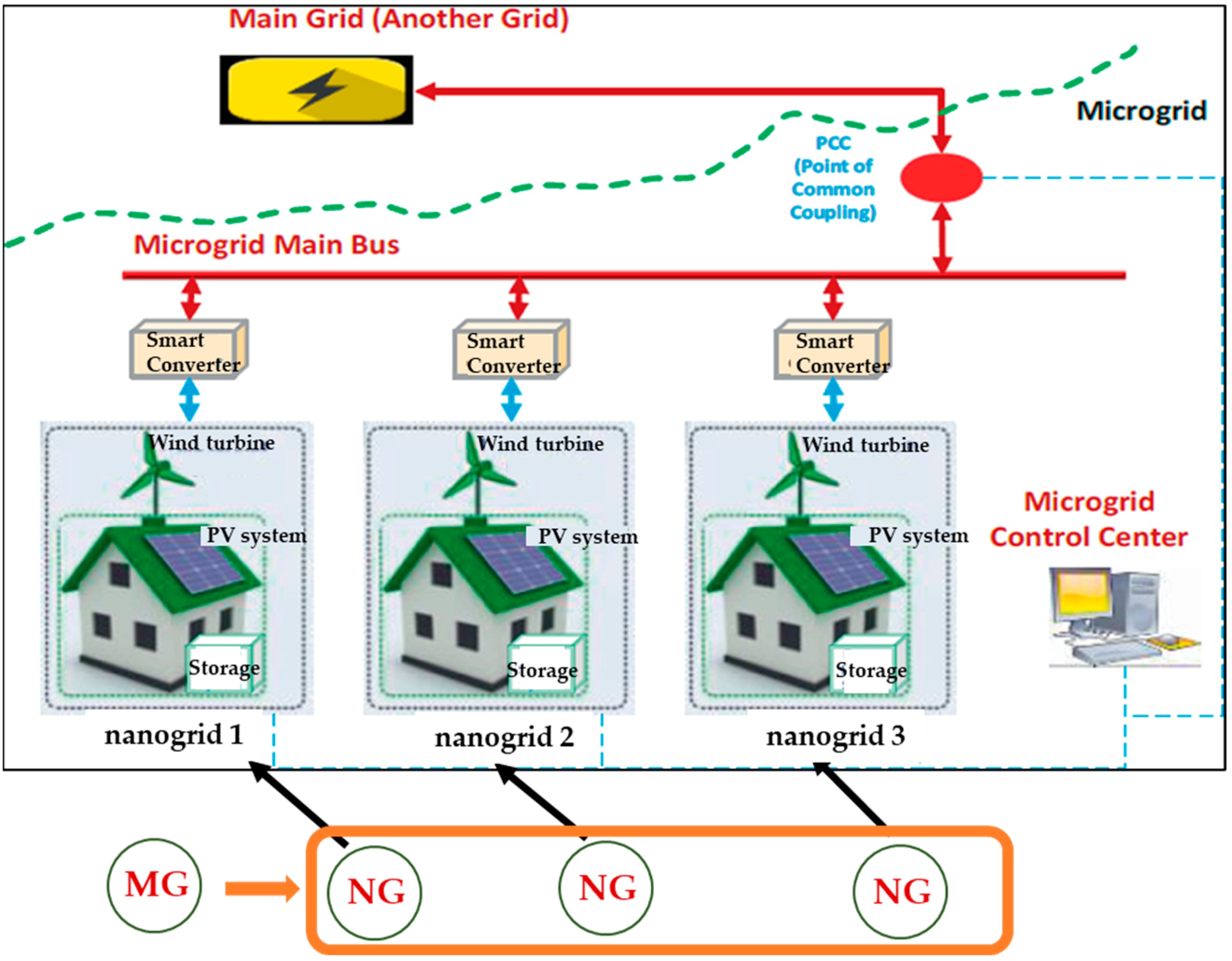
Nanogrid in this paper refers to a single house, as shown in Figure 1, which has the capacity to transact energy with the grid and other connected nanogrids as shown in Figure 1. Moreover, it has photovoltaic (PV) panels, a small wind turbine, and the grid as energy sources that power the electrical appliances (cooling and heating system, lighting system, an electric pump, dishwasher, washing machine, microwave, and oven, and refrigerator) having an operational load of not more than 10 kW.
Load Forecasting is not a novel concept as it has been extensively used for micro-grid where numerous methods have been developed and employed as mentioned in [5,6,7,8,9,10,11]. These methods are focused on smooth loads that are aggregated from its connected load centers such as residential areas, commercial complexes, or industries. This aggregation damps all the variations which might have been caused by sudden and frequent switching on or off electrical appliances. This abrupt load behavior, which is very prevalent in a nanogrid makes its load forecasting a daunting task and has not been studied in detail [12,13]. Therefore, the existing load forecasting models, developed for micro-grid, need further consideration for their suitability in nanogrid.
Furthermore, as nanogrid experiences frequent load perturbations [13], this may cause Peak to Average Power Ratio (PAR) to fluctuate frequently. This will raise the energy cost of a nanogrid, especially when appliances are operated during peak hours of the day. It is estimated that 30–70% of energy cost is associated with peak load demand in the USA [14]. However, through proper load scheduling techniques, energy costs can be minimized [15]. These techniques include load shifting and peak shaving [16,17,18], which are mostly employed for micro-grids and grids. Therefore, studies investigating the economic impact of peak shifting in a nanogrid, are few, which motivates us to align our load forecasting model in determining its impact on daily energy cost. This paper, as explicated in Section 3, is focused on two parts, i.e., load forecasting, and its utilization in ascertaining potential savings by decreasing peak to average power ratio (PAR): peak load shifting from peak hours to off-peak hours. Due to the high dependency on meteorological data for accurate load forecasting, dominant weather parameters have been extracted using the correlation technique in the first part of our research. In addition to this, the time-lag value of 1(t-1) has also been considered to maintain the momentum of the load. Thus, an ensemble of features has been used as an input to predict an hour-ahead load forecasting. In the second part of our research, peak load is identified from the prediction by comparing it with an average of the previous load. If the predicted load occurs in peak hours and is greater than 1.5 times the previous averaged load, then it is considered a peak load. Based on this, estimates have been made as to how much savings will be by shifting the load to off-peak hours based on the peak and off-peak hour pricing system.
To quantify the model accuracy and consequent savings, model simulations have been performed using the data, obtained from [19], which results in load prediction with an MSE of 0.03 kW and an average of 20% savings in load shifting. Moreover, the model has been compared with Long Short-Term Memory (LSTM), Gated Recurrent Unit (GRU), and Bi-directional Long Short-Term Memory (Bi-LSTM) models as well. Detailed results have been discussed in Section 4.
The contributions of this paper are summarized below:
- A multi-layer perceptron model with dynamic feature selection is developed for hour-ahead forecasting of a nanogrid;
- Peak loads of a nanogrid are identified fast and accurately based on the predicted load for potential energy cost saving through load shifting;
- Numerical testing results demonstrate the performance of the developed model with MSE of 0.03 kW, MAPE of 9%, and CV of 11.9%, and the achievement of 20% energy cost savings through shifting peak loads throughout the day.
2. Literature Review
This section deals with a review of existing models relevant to load forecasting and the identification of peak loads. Since little research has been found on nanogrid load forecasting; therefore, in Section 2.1, existing load forecasting models for microgrid and grid have been reviewed and in Section 2.2, studies relevant to the detection of peak loads have been analyzed.
2.1. Load Forecasting
Extensive research has been conducted in the field of Short-Term Load Forecasting (STLF) for microgrids and the grid, which is majorly based on one of two methodologies: Statistical methods and Machine Learning algorithms [20,21].
In [22], the author compares three different algorithms (Seasonal Auto-regressive Integrated Moving Average (SARIMA), Artificial Neural Network (ANN), and Wavelet Neural Network (WNN)) to determine which methods perform better for load forecasting. Upon comparison, it has been found that the statistical method, i.e., SARIMA, underperforms in comparison to the machine learning methods, i.e., WNN and ANN. This is due to its limited ability to incorporate variations and fluctuation of load. Thus, the author concludes that for more chaotic loads, machine learning methods such as neural networks perform better.
In [23], ANN is implemented on the ISO New England-NEEPOL dataset using exogenous parameters such as temperature, humidity, and wind speed. Similar work has also been presented in [24], in which an LSTM-based model has been presented that predicts load forecasting using data from ten substations of Beijing city. Moreover, researchers have been implementing hybrid algorithms to improve the efficiencies of the prediction models. A similar methodology has been implemented in [25], where a hybrid approach of combining two algorithms, Best-Basis Stationary Wavelet Packet Transforms and Harris Hawks optimization-based Feed-Forward Neural Network, has been discussed. By applying these models, errors in micro-grid STLF were reduced by 33.3%, 49.5%, and 60.76% in comparison to Particle Swarm Optimization (PSO), Support Vector Machine (SVM), and back-propagation-based neural network, respectively. In [26], Support Vector Regression (SVM) and LSTM have been combined to predict the short-term (3-day ahead) load forecasting of a microgrid. In [27], the authors predicted the short-term load by dividing the data into clusters of customers, having similar load values, and then, load forecasting is done. Again, the results rely on aggregated data, thus producing a “smooth” aggregated load [22].
In addition to this, Table 1 further summarizes more work for STLF, involving a plethora of algorithms, such as ANN, LSTM, ARIMA, Linear Regression (LR), Gradient Boosted Regression Trees (GBRT), GRU, Support Vector Regression (SVR), Recurrent Neural Networks (RNN), etc.
With different algorithms, the accuracy of models has improved a lot, but with ever-increasing complex networks, in which more chaotic systems such as nanogrid, are entering, such models might not be able to incorporate higher load variations. This is also corroborated in [29], in which high variability in nanogrid load and difficulty in load forecasting has been observed by authors. For short-term load forecasting, authors have implemented various machine learning techniques on a nanogrid, and it is concluded that Artificial Neural Networks perform better than other algorithms, i.e., LR, SVR, Convolutional Neural Network (CNN), etc. Moreover, it has been found that statistical models, i.e., ARIMA, LR, Multivariate Regression Analysis, etc., are computationally simpler models, but these cannot assimilate the sudden variations in their input [30]. The ANN can handle it due to the hidden layers which can map the data more efficiently [31,32], which is also evident in its usage in diverse fields such as scheduling of energy storage [33], intrusion detection, and cybersecurity [34], supply chain management [35], pattern recognition, weather forecasting [36,37], renewable generation prediction [36], predictive maintenance for wind turbines [38], etc. Due to such reasons, ANN is best suited for handling nanogrid load.
For this paper, ANN has been chosen, but it is also important to choose the optimizer to improve the efficacy and accuracy of the model. This approach has been utilized in [39,40] by utilization of various meta-heuristics optimizers for optimization of the model’s parameters. The authors of [40] compare two ANN models, one with a PSO-based optimizer and the second with a humpback whale optimizer for the prediction of efficiency and water output for tubular solar still. Results show that the optimized model with humpback whale optimizer performed better than the other model. Performance with and without moth-flame optimizer has been compared in [41] for productivity forecasting of solar distiller using an LSTM model. Based on findings, it is evident that LSTM with optimizer performs better. Thus, it is established that an optimizer is important for accurate and quicker convergence. Moreover, in electrical load forecasting, a gradient-based optimizer is broadly used [42,43], and this optimizer is also combined with RMSProp Optimizer in conjunction with the Momentum. Such a combination, also known as Adam Optimizer, converges faster. Therefore, Adam Optimizer has been used for the ANN model presented in this paper.
2.2. Peak Load
Alone load prediction, without translating it into economic or technical benefit, will be of little use to stakeholders. Therefore, peak load detection has been one of the key focus areas in load prediction. It is among the major issues which impact an entire electric network; therefore, various methods have been developed to detect peak loads and manage them such that PAR is reduced, which is a win–win situation for both consumers and operators. The authors of [8] focus on peak load prediction in a micro-grid. For detection, the authors first chose RNN-LSTM to forecast demand and then, used the model to predict the peak load. Additionally, the authors also used LR, ARIMA, and ANN for comparison with the LSTM-based model. Amongst all these models, the LSTM-based model performed best. In addition to this, the authors of [44] have generalized the prediction model by combining outputs of ensemble models, i.e., AdaBoost, Bagging and Boosting, Random Forest, and gradient boosting, and the compensation technique for small industries. Their work focused on peak load prediction for two factories. By applying ensemble models only, accuracy was very poor but when “compensation constant” was applied during the testing process, accuracy improved. Such peak detection methods have been widely used in micro-grid for reducing the energy cost which resonates in [45], where the author has immaculately summarized the potential benefits of peak detection and consequent demand response, in improving power quality, minimizing losses, and optimizing the cost of operations in both micro-grid and the grid. Furthermore, in [46], an algorithm predicting peak electric load days (PELD) is implemented using ARIMA and Neural Networks (NNs). The research was primarily focused on the prediction of peak days, but for this, load forecasting needs to be performed first. Therefore, simulations were performed with combinations of both mentioned algorithms on a set of commercial buildings, having a smoother load, unlike nanogrid.
In short, all the above-mentioned works are based on either a micro-grid or the grid’s load which, according to [47] has a certain pattern and damped variations due to the collective effect of loads. Thus, the existing STLF models might not be sufficient for load prediction and consequent peak detection in a nanogrid, where variations are more prominent due to the granular nature of demand [13] and load does not always follow the smooth curve as a micro-grid, or the grid does [47].
Therefore, this paper implements the ANN model with t-1 load and meteorological parameters in the first part, and then, based on peak load predictions, economic benefits are determined when peak load shifts from peak hours to off-peak hours.
3. Methodology
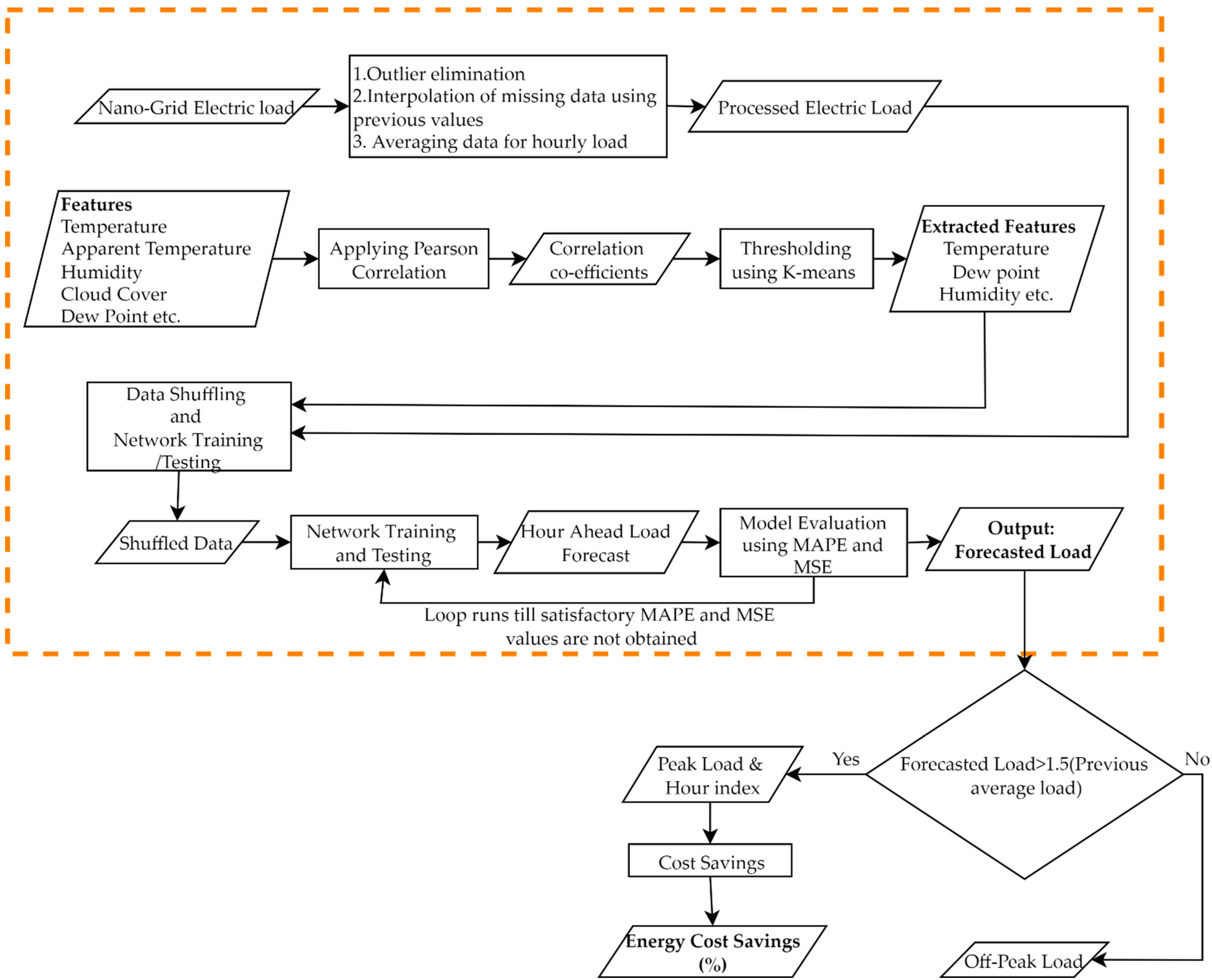
This section contains a summary of the developed model, which includes data handling, feature selection, modeling of neural networks, model evaluation criteria, and energy cost savings.
3.1. Pre-Processing
Data are, initially, pre-processed so that any outliers, which might skew the results, are excluded from the training samples. In addition to this, electric data are also lost during sampling from smart meters, which might result in erroneous or zero values. Such issues have been solved by taking an average of the previous two hours’ electric load, assuming that no new appliance or equipment has been turned on in that hour. A similar issue can also arise during the collection of weather parameters which includes include Temperature, Apparent Temperature, Humidity, Dew Point, Wind speed, etc. Thus, this process is not only specific to electric load but is also applied to weather features as well.
Furthermore, to incorporate the granularity for hour-ahead load prediction, date-time stamps have been decomposed at an hourly level. The previous hour’s load (t-1) and the slope have also been considered as potential input features such that the load momentum can be incorporated. The reason to include t-1 is due to fact that electric load tends to have momentum as it tries to maintain the previous instant’s value. To emulate this behavior in our work, the “t-1” variable is introduced which represents the previous hour’s electric load value. The reason to choose the previous hour’s load is that our work deals with hourly load prediction. Had it been a 15-min ahead load prediction, we would have chosen the previous 15-min value. Moreover, the slope is associated with the hourly change rate of electric load. The greater the change in electric load, the larger the slope. All the features are then passed through the feature selection method, defined in 3.2 which extracts the dominant features.
3.2. Feature Selection
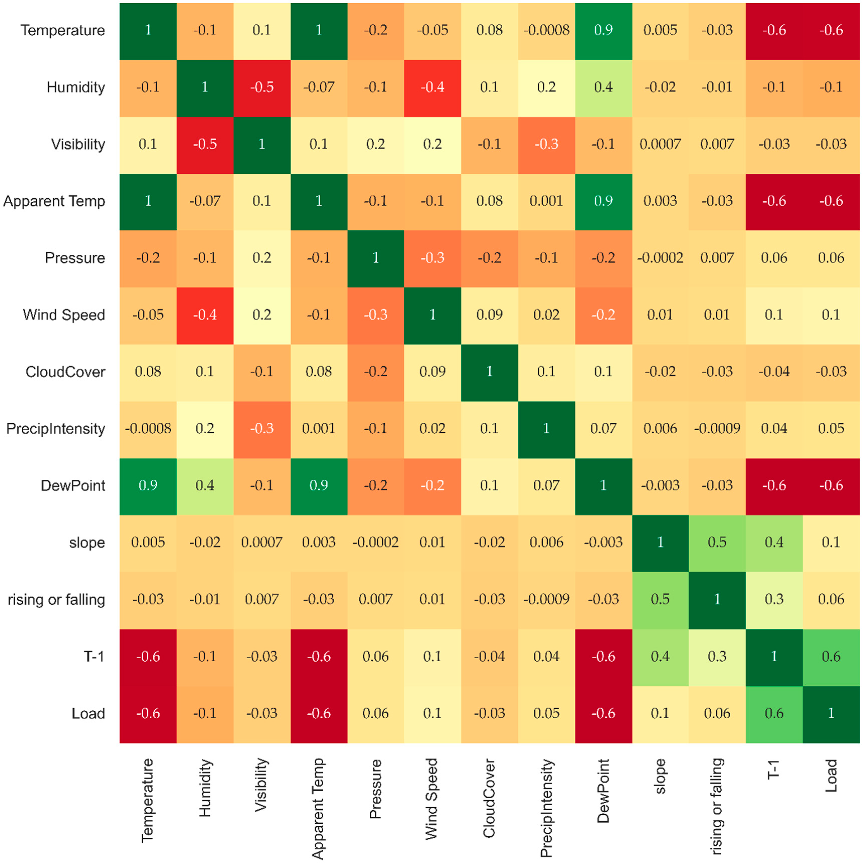
Since the load either increases or decreases with varying meteorological inputs, it is necessary to have a correlation technique that can incorporate relations in both negative and positive directions. To draw these relationships, various correlation techniques are employed, such as Pearson, Spearman, Kendall, etc. Among them, the Pearson Correlation is the widely used technique [48,49,50] as it provides the linear relationship (negative or positive) between input parameters with the target values, while Spearman and Kendall provide a monotonic association between the input and target. Therefore, the Pearson coefficient is considered in this work.
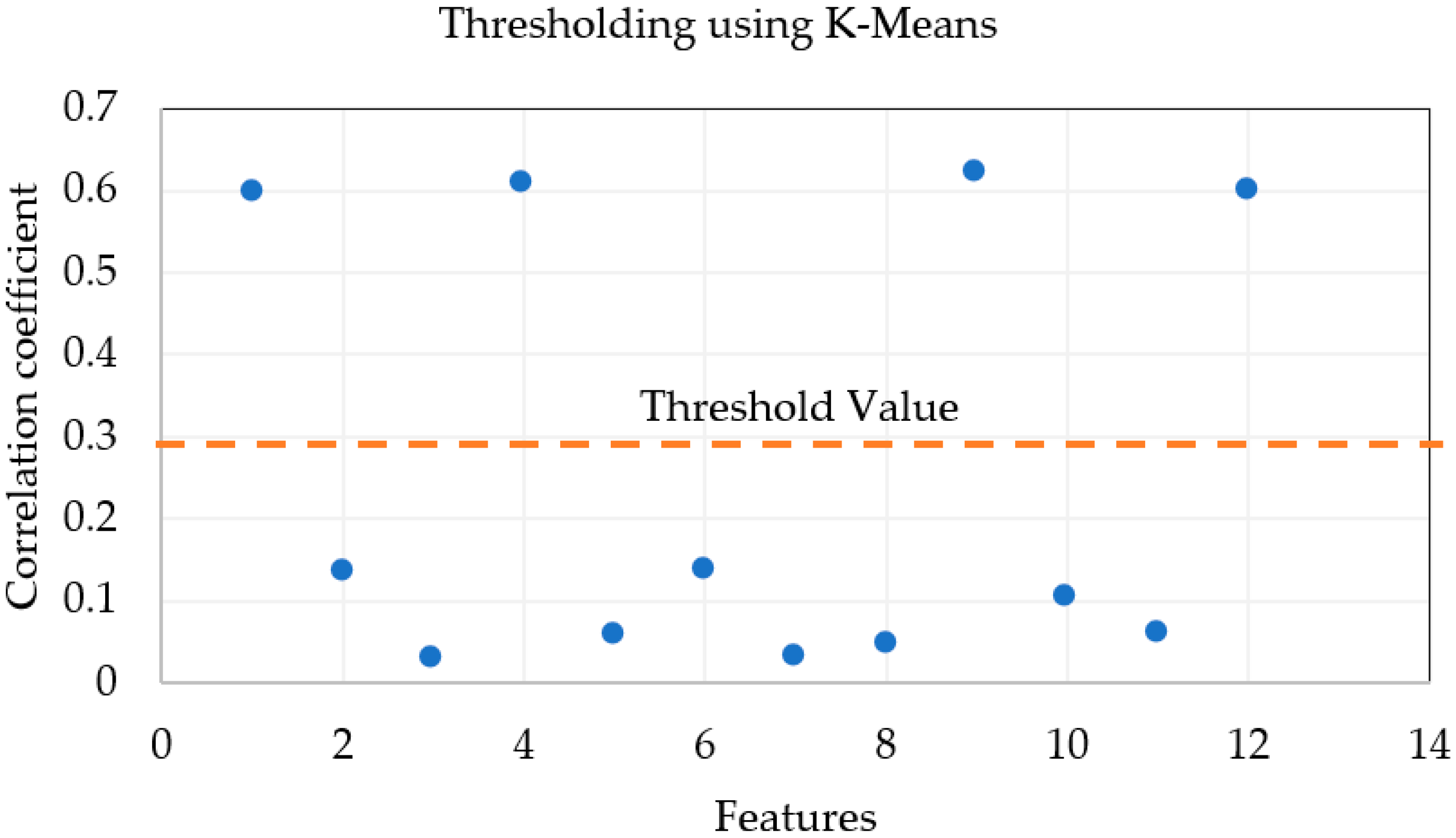
The higher the value of Pearson coefficient, the higher the impact it will have on the electric load. The threshold for correlation coefficients has been determined using the K-means clustering method, in which correlation coefficients are divided into two clusters. The midpoint between the centroids of two clusters is considered a threshold for the correlation coefficients. This means that correlation coefficients lying below the threshold are considered insignificant and values above the threshold are deemed impactful and selected as an input feature. A similar concept has been presented graphically in Figure 2, in which the features corresponding to abscissa values of 1 (Temperature), 4 (Apparent Temperature), 9 (Humidity), and 12 (t-1 load value) are above the threshold values. These will be selected as input features while the remaining are dropped out.
It is also observed that either increasing or decreasing the number of input features impacts the model accuracy significantly. Decreasing the input features deprives the model of the nuances of data and increasing the features overfits the model. Therefore, features have been selected by observing the values of MAPE and MSE such that error is minimized.
Selected features and electric load are then passed through a machine learning model for load prediction.
3.3. Network Modelling
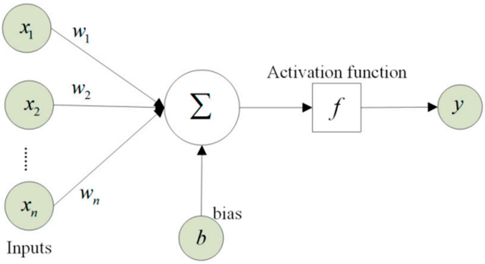
An artificial neural network is a computational method that can take a number of complex inputs and determine the relationship in between input and output for predictions using the neurons. Each neuron has three components i.e., weights (Wn), input (xn), and activation function (f) and bias (b) as shown in Figure 3. Inputs coupled with weights are passed into an activation function to determine the output (y).
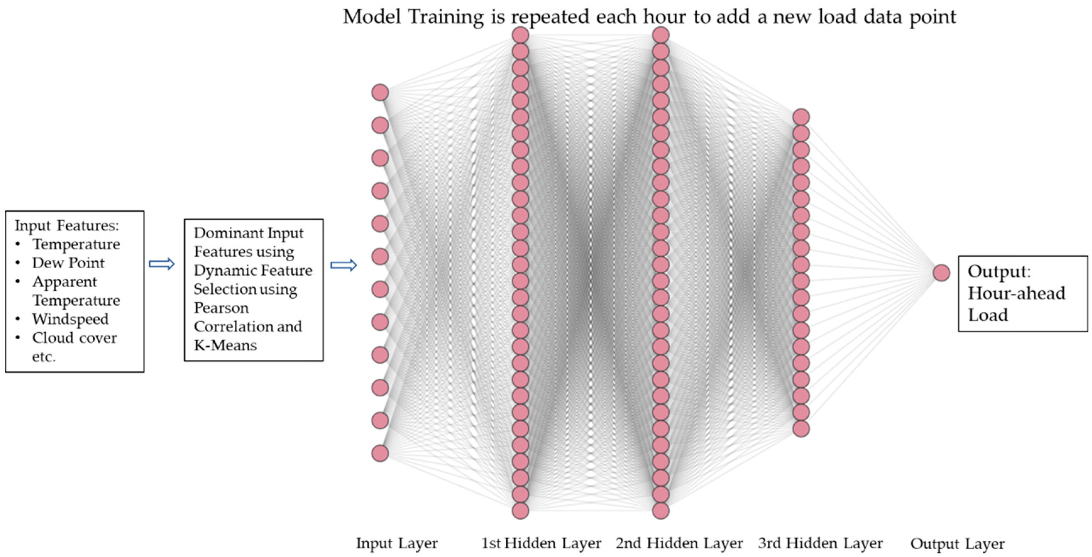
For the network modeling, the ANN model, as shown in Figure 4, has been used which has an input layer containing input features and an output layer that predicts hour-ahead load. In between the input and output layers, there are three hidden layers, each containing an activation function. Since, Rectified Linear Unit (ReLU) is the most widely used activation function [51] amongst other functions such as Binary Step Function, Leaky ReLU, Sigmoid, Linear, and Tanh, etc.; therefore, it has been utilized, which is defined as (1):
where x represents the input features such as temperature, humidity, windspeed, etc., for the particular neuron, while y shows the output of that particular neuron which can be either zero or a positive value.
Processed load data obtained using the method mentioned in Section 3.1 and extracted features using the method described in Section 3.2 are compiled. Consolidated data are then shuffled and divided into training and testing datasets with an 80:20 ratio. Based on the set hyperparameters, the model is trained and then tested. Based on MAPE and MSE values, training is re-iterated with updated hyperparameters, and this process goes on until satisfactory MAPE and MSE are not obtained.
Once satisfactory values of MAPE and MSE are obtained, the model is tested on the test data. This gives the forecasted load, which is then compared with the average load of previous hours of that particular day. If the forecasted load is higher than the average by 1.5 times and lies within peak hours, then it is classified as a peak load. Once the peak load is identified, energy cost savings are determined by shifting the peak load to off-peak hours. For each peak load hour, the amount of load shift to off-peak hours is equal to the difference between this peak load and an average of previous hours’ load.
3.4. Pseudocode
Pseudo-code of the ANN-based model is given below as Algorithm 1 and the pseudo-code along with a description and methodology of the remaining methods i.e., LSTM, GRU, Bi-LSTM is presented in Appendix C, Appendix A, and Appendix B, respectively.
| Algorithm 1: for the ANN Model | |
| Input: Input features i.e., Meteorological data and Electric load | |
| Output: Hourly forecasted electric load and daily energy cost savings | |
| 1. | Get weather and electric load data |
| 2. | Pre-process the data by converting electric data into hourly electric data |
| 3. | Extract slope, t-1 load, and “rising or falling edge” parameter from the electric load |
| 4. | Get Pearson correlation Coefficients (µf) for weather data and its corresponding electric load |
| 5. | Apply K-means with K = 2 on the set of coefficients [µ1, µ2,...,µf] and determine the mid-point of two centroids (m) |
| 6. | for (t < Number of Potential features) |
| 7. | if (µf > m) |
| 8. | Feature (f) is selected as an input feature |
| 9. | else |
| 10. | Feature (f) is dropped |
| 11. | t = t + 1 |
| 12. | end for |
| 13. | Divide data (Input feature and electric load) into training and testing sets |
| 14. | Initialize ANN model |
| 15. | Training time starts |
| 16. | while (1) |
| 17. | Run the model |
| 18. | Losses are calculated |
| 19. | Tune the hyperparameters if needed |
| 20. | if1(Losses(t)-Losses(t-1)< ε) |
| 21. | count = count + 1 |
| 22. | if2 (count > β) |
| 23. | Break |
| 24. | end if2 |
| 25. | end if1 |
| 26. | end while |
| 27. | Training time stops and total training time is calculated (time) |
| 28. | Model tested on test data for hourly load forecasting (Lhour) |
| 29. | MAPE, MSE, CV, and RMSE are calculated |
| 30. | if (Lhour > 1.5*average (Lprevious_hours) & time is within range of peak hours) |
| 31. | Lhour is considered peak load |
| 32. | end if |
| 33. | Savings are calculated based on the potential shifting of Lhour to an off-peak hour. |
| 34. | Repeat from point 4 for load forecasting of the next hours |
3.5. Model Evaluation Criterion
To measure the performance, Mean Absolute Percentage Error (MAPE) is commonly used [26,47]. It calculates the means of the difference in the forecasts and the actual value and mathematically it is shown as (2). Additionally, mean square error (MSE) and co-efficient of variance (CV) [53] are also used, which is calculated by (2) and (5), respectively.
where is the actual load data at hour i, is the output of the forecasting model at hour i, and is number of data samples.
4. Results
This section presents the summary of the data being used, hyperparameters for the NN model, selected input features, load forecasting, and potential savings in energy cost. The model has been implemented in Python 3.9 and simulation is performed on a MacBook Pro with a 2.6 GHz Dual-Core Intel i5 processor and system memory of 8 GB 1600 MHz DDR3. Upon simulation, the nanogrid load has been forecasted with an MSE of 0.03 KW, MAPE of 9%, CV of 11.9% and potential savings of 20% by peak load shifting.
4.1. Dataset Description/Set-Up
An online dataset with electric load of 146 apartments and weather data from the Laboratory for Advanced Software Solutions [19] is utilized. In our case study, a single apartment with two years of load data is considered. The sampling frequency of load is one minute while the weather data have a one-hour sampling frequency. Therefore, to synchronize both, load data have been averaged over an hour. As discussed in Section 3.1, slope and previous hour’s values have also been used and considered as potential input features.
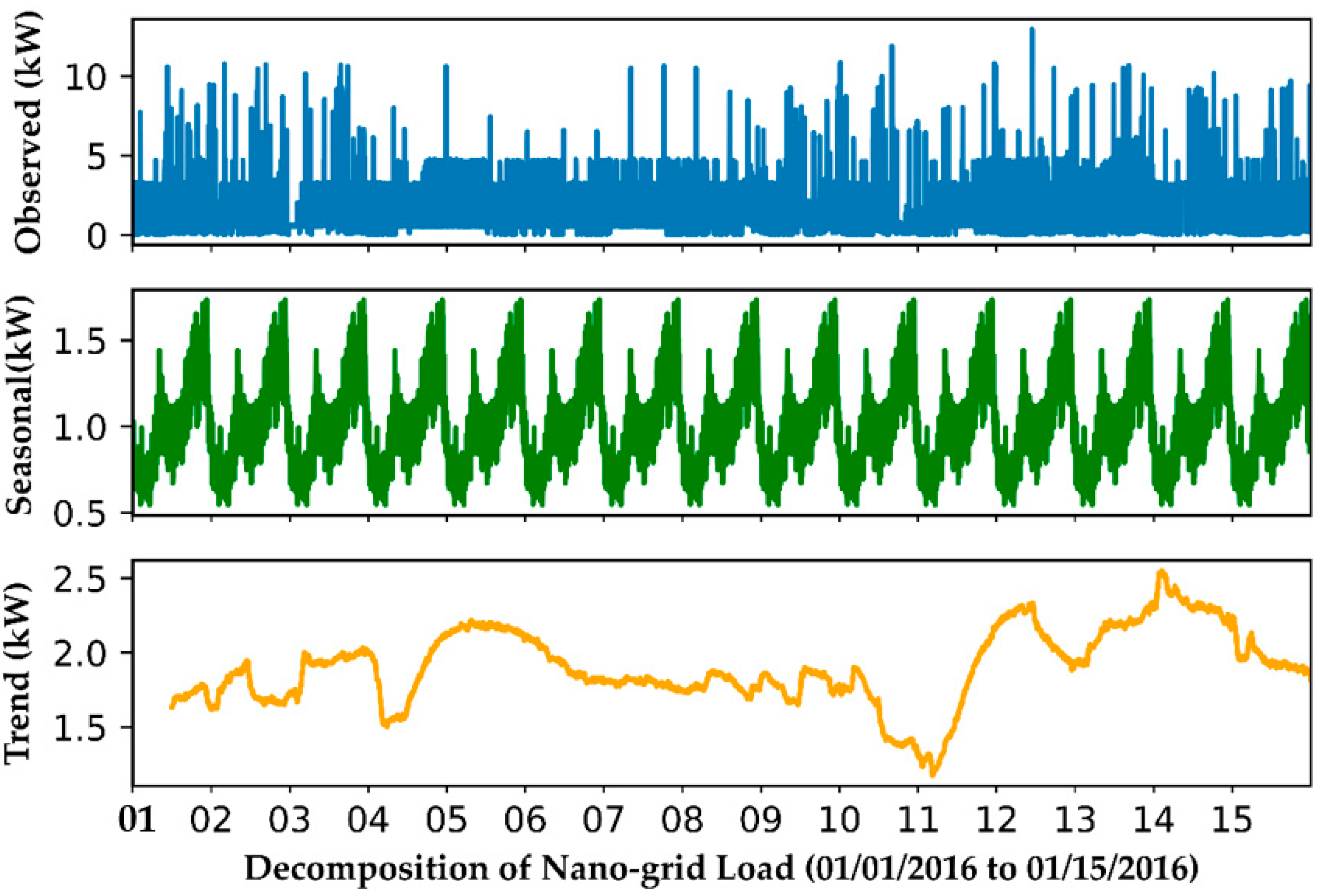
Furthermore, load data have been decomposed into observed, trend, and seasonality. To show load variations, the decomposed data from 1 January 2016 to 15 January 2016 have been plotted in Figure 6 as an example, in which it is evident that the load does not have a daily trend or specific pattern on a day-to-day basis; unlike gird or microgrid [47,54]. In addition, seasonality can be observed on a day-to-day basis, and it oscillates from −0.5 kW to 0.5 kW, which also shows that load has variability. This makes data prediction harder in nanogrid as mentioned in Section 1.
Weather features in the dataset are Temperature (°C), Apparent Temperature (°C), Humidity, Cloud Cover, Dew Point, Pressure (Bar), Wind Speed (m/s), Visibility, and Precipitate Intensity. Their filtering is discussed in the next Section 4.2.
Lastly, peak and off-peak hours of Western Massachusetts have been considered. From June to September, peak hours are 9:00 a.m. to 6:00 p.m., and from October to May, peak hours are 8:00 a.m. to 9:00 p.m. [55], as to be highlighted in grey later in Figure 11 and Figure 12, respectively.
For the peak and off-peak hour pricing system under consideration, the unit cost of energy is $0.006/kWh and $0.005/kWh for peak and off-peak hours, respectively.
To demonstrate the performance of the ANN-based model, it is compared with three widely used forecasting models including LSTM, GRU, and Bi-LSTM. For LSTM, GRU, and Bi-LSTM models; input data are the time-series electric load [19] of a nanogrid, and output is the hourly load forecast.
4.2. Hyperparameters and Features
For neural networks, three hidden layers with ReLU, as an activation function, have been configured with a learning rate of 0.0001 and 300 epochs. In the first and second hidden layers, there are 30 fully connected neurons and in the third, there are 20 fully connected neurons.
For features extraction, a correlation coefficient map has been obtained by performing Pearson Correlation on the features as shown in Figure 7. Obtained correlation coefficients are compared with the threshold value, which is 0.34 for this particular testing. If the coefficient is greater than 0.34, then the feature is considered an impactful feature that affects the electric load. Based on this, Temperature (°C), Apparent Temperature(°C), Dewpoint, and t-1 load (kW) have been selected. After the feature selection, data are divided into training and testing subsets with an 80:20 ratio. Training samples are then passed into the neural network model.
Each model, i.e., LSTM, GRU, and Bi-LSTM, has one hidden layer with 200 internal units, a learning rate of 0.001, and Adam as an optimizer. These three models were simulated for 10 epochs. Moreover, the model parameters of all four models have been tabulated in Table 2.
4.3. Load Forecasting
Using the developed model, simulations, with the training time of 7 min and 36 s, are performed on the test load. Hour-ahead load is predicted with an MSE of 0.03 kW and MAPE of 9% as tabulated in Table 3. In addition to this, the model is also compared with the LSTM model which initially gives an MSE of 0.54 kW and MAPE of 37%. Since these results are larger than that of the ANN model, LSTM hyperparameters have been further tuned for a fairer comparison. Tuning the parameters improves the performance from 37% to 28% but it took more than 30 min which is quite computationally expensive. Computational time plays a major role in STLF forecasting [56]; therefore, the LSTM model is not selected for further consideration in our work. Furthermore, GRU and Bi-LSTM were also used to compare their results with developed model. Both models were computationally expensive and lesser accurate than the ANN -based model.
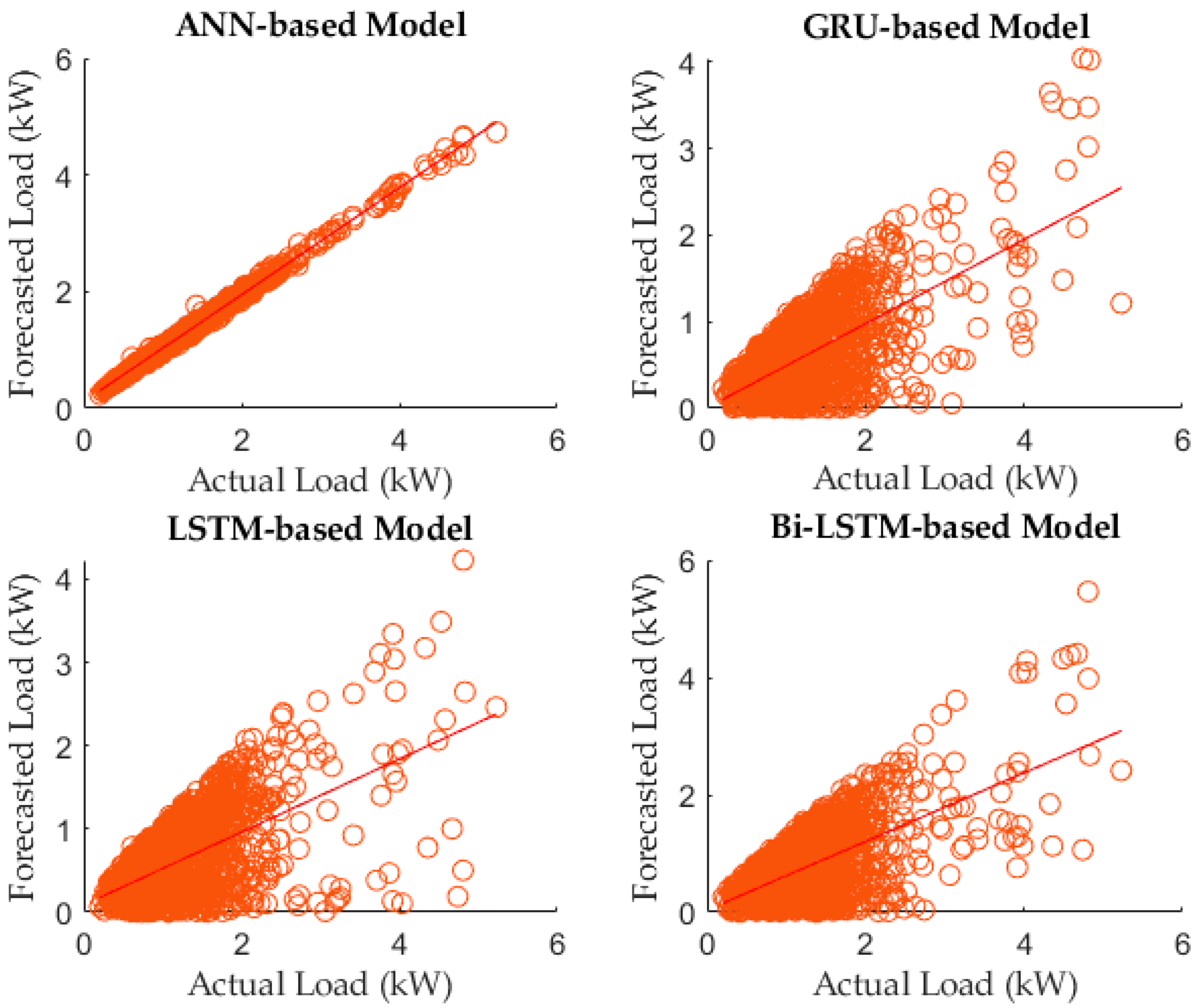
Scatter plots for each model’s predictions are presented in Figure 8. The figure shows that the error between the actual and forecasted load obtained from the ANN-based model is much smaller than those from the other three models.
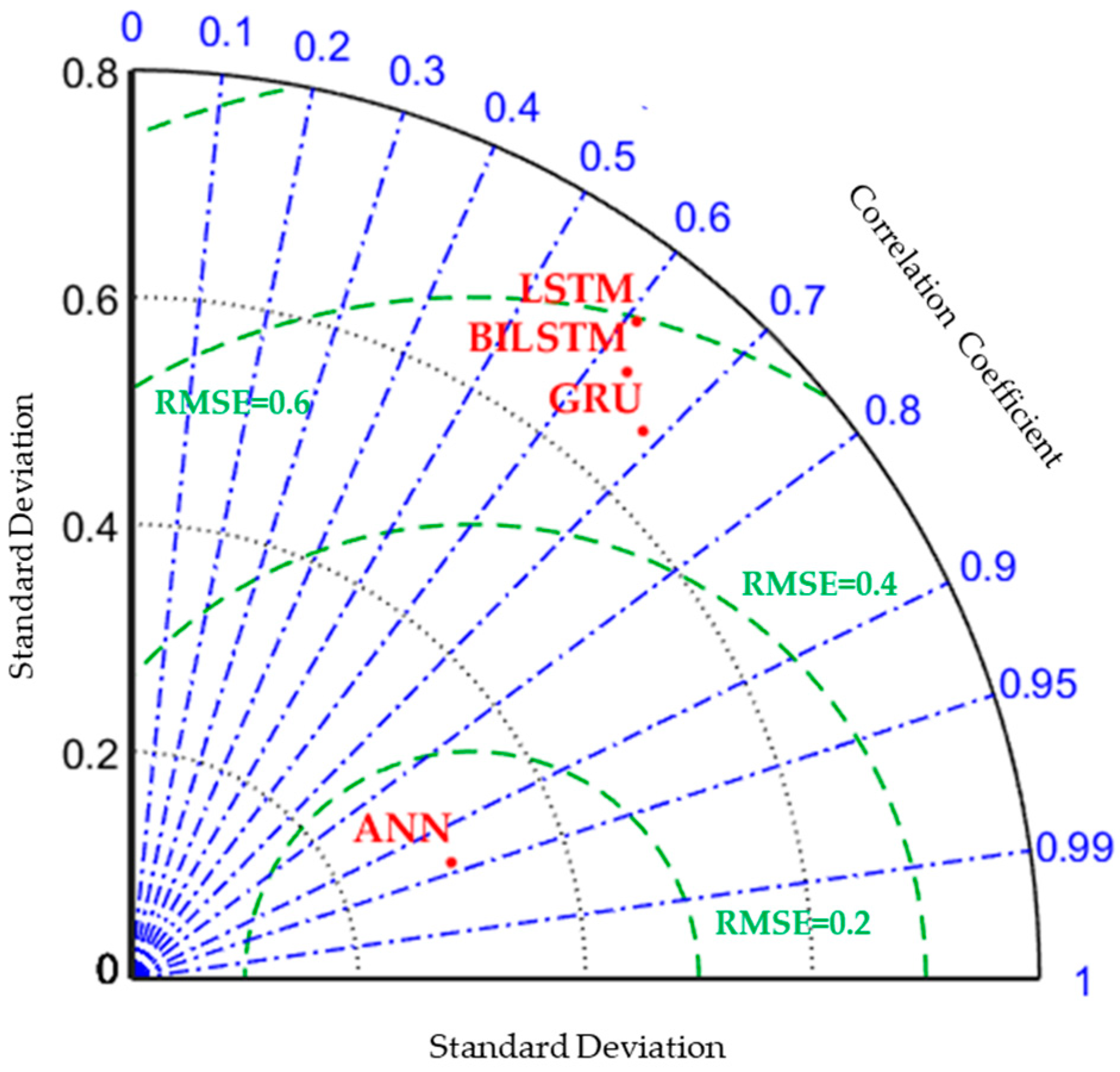
In addition, to further compare the ANN-based model with LSTM, GRU, and Bi-LSTM, the Violin plot and the Taylor diagram are shown in Figure 9 and Figure 10, respectively. A comparison has been made between the distribution of actual load data points with the distributions of predicted load data points obtained from four models. As shown in Figure 9, the actual load has the highest distribution from 0.5 kW to 2.5 kW with a median of 1.19 kW. The ANN-based model has a similar distribution within the same range and the median is almost the same (1.2 kW). LSTM, GRU, and Bi-LSTM models have densely populated points between 0.5 kW to 1 kW with medians at 0.27 kW, 0.16 kW, and 0.162 kW respectively. The above results demonstrate the ANN-based model is more accurate than the three models.
From Figure 10, it is evident that ANN performs better with the least RMSE of 0.17 kW and the highest correlation of 0.95 with the actual load. For LSTM, GRU, and Bi-LSTM, their correlation coefficients (0.6, 0.63, and 0.69, respectively) are smaller and their RMSEs (0.60 kW, 0.55 kW, and 0.59 kW, respectively) are larger as compared to those mentioned above.
From the above plots in Figure 8, Figure 9 and Figure 10, the ANN-based model has better performance in comparison to other models.
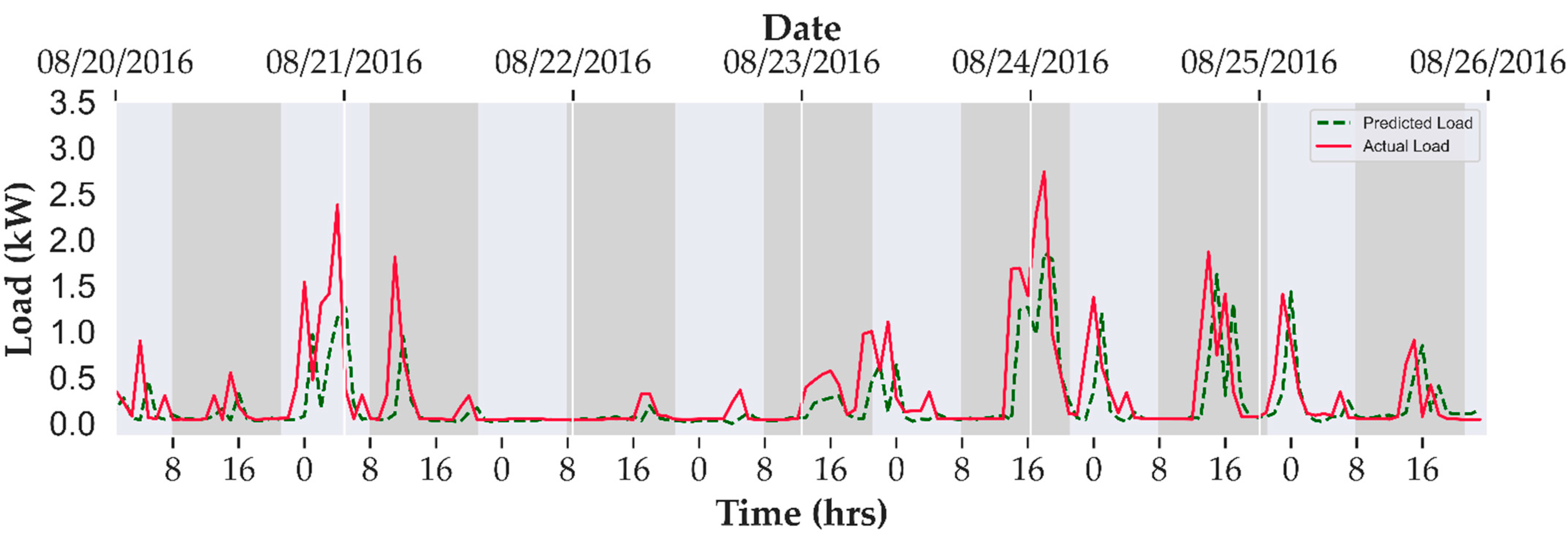
Moreover, simulations are also performed for different weather conditions so that model can be rigorously tested, and its robustness can be demonstrated for seasonal changes. Therefore, a winter week and a summer week are taken as test cases. For the winter season, a week of January is chosen in which temperature drops below −8 °C, and for summer, a week of August is chosen because of higher temperatures. Furthermore, the reason to choose a week is to test the model on weekdays and weekends. Results for the summer and winter weeks are shown in Figure 11 and Figure 12, respectively.
Figure 11 shows the actual and predicted load values for a summer week. Here load varies from a few watts to 3 kW with peaks on some days and flat on some days. The flat load might be due to lesser occupancy on those days. Nevertheless, the model manages to differentiate between the peaks and flat load and predicts load forecasting with an MSE of 0.18 kW. Such a high MSE value, in comparison to the weekly average load of 0.11 kW, is due to lower data points, showing the transition from very low loads, almost equal to zero, to peak loads. It is to be noted that Figure 11 is a seven consecutive day graph, in which each hour is forecasted and then appended to the graph to show the variations all along the week and model performance.
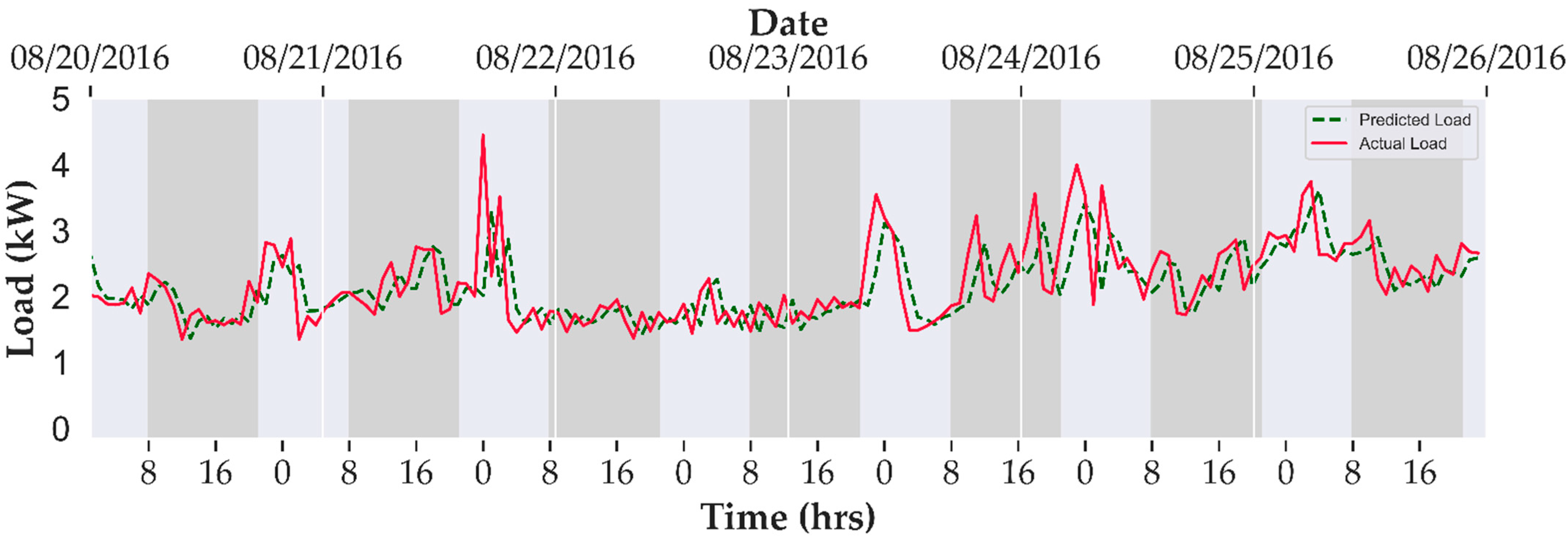
Figure 12, which shows load forecasting for a winter week, has also been plotted in the same manner as Figure 11. As the winter season is more extreme in comparison to the summer season in Western Massachusetts, it can be observed that the average load has increased and now it hovers around an average load of 2.18 kW with peaks touching approximately 5 kW. Even due to more variations and changes in seasonality, the model still predicts the load with accurate peak hours with an MSE of 0.27 kW.
4.4. Cost Savings
A typical summer week is used to determine the potential cost savings when peak loads, as identified through the model, are shifted to off-peak hours. It is a known fact that the unit cost at peak hours is always higher than that of off-peak hours; therefore, shifting the load will lead to cost savings which are corroborated in Table 4.
From Table 4, it is evident that reduction in PAR, which is the by-product of peak shifting, results in cost savings ranging from 19% to 25%. Thus, it can be conservatively stated that a daily 20% energy cost can be saved if peak loads are correctly identified and notified with accurate hour indexing.
Moreover, weekly savings for other months of the year have also been determined as shown in Table 5. The first row (Extreme Summer) shows the weekly savings of 16.7% in July, a month considered hot in Western Massachusetts. The second row (Extreme Winter) shows weekly savings of 8.85% for January, which is considered among the coldest months. Thus, extreme cases have been tabulated. It is to be noted that during the Extreme Winter week, heavy appliances were not operated frequently during peak hours. This means that during the peak hours, the load was relatively stable with lesser spikes. Due to this reason, the difference between the hour-ahead forecasted load and the previous hours’ average load was small. Therefore, low energy savings of 8.85% in the Extreme Winter week have been observed as compared to that of 16.7% in the Extreme Summer.
Based on cost savings results, it can be approximated that for the nanogrid considered in this paper, energy cost savings (%) for a year would be approximately 15.18%.
5. Conclusions
Most of the foresting studies have been focused on the micro-grid and grid loads, which are stable and have patterns throughout the day. Our work focuses on forecasting of nanogrid load which has an enormous amount of variability. To capture this variability, weather features and the previous hour’s load (t-1) load have been used. Using these features, which have been extracted using the correlation technique, an ANN-based model has been developed which predicts load with MSE of 0.03 kW, MAPE of 9% and CV of 11.9%. Furthermore, peaks loads with time indices are determined, which results in 20% energy cost savings if peak loads are shifted to off-peak hours. The main advantage of our model, in comparison to existing load forecasting studies, is its capability to handle large load variability which is proved by testing it on different seasons and results show consistent savings in all, which proves that the developed method surpassed the realms of seasonality. Meanwhile, a concern is its reliance on the accuracy of the localized weather data, which might cause instability in the nanogrid if the weather data are not accurate enough. This might not happen in grid or microgrid as these are bigger systems and can handle such inaccuracy in a better way.
There is a growing trend of energy transactions between nanogrids. Such transactions require accurate information of an hour-ahead load to ascertain the flow of energy between nanogrids. Moreover, whether a nanogrid will have energy in surplus or deficit can be determined by load forecasting and implemented load shifting strategies, which becomes helpful in deciding the energy price of that nanogrid within the network.
Based on the above discussion, future work could be:
- Apply optimization methods to decide load shifting strategies and, thus, to determine penitential energy cost savings for a nanogrid;
- Optimize the pricing mechanism for energy transactions within the nanogrid network by using the developed load forecasting model.
Author Contributions
Conceptualization, B.Y. and A.K.; methodology, A.K. and B.Y.; software, A.K.; validation, A.K.; investigation, A.K., A.B. and B.Y.; data curation, A.K. and A.B.; writing—original draft preparation, A.K.; writing—review and editing, A.K., A.B. and B.Y.; visualization, A.K.; supervision, B.Y.; project administration, B.Y.; funding acquisition, B.Y. All authors have read and agreed to the published version of the manuscript.
Funding
This work is supported in part by the donation from Micatu, Inc.
Institutional Review Board Statement
Not applicable.
Data Availability Statement
Not applicable.
Conflicts of Interest
The authors declare no conflict of interest.
Abbreviations
Following abbreviations have been used in this paper:
| ANN | Artificial Neural Network |
| ARIMA | Autoregressive Integrated Moving Average |
| Bi-LSTM | Bi-directional Long Short-Term Memory |
| CNN | Convolutional Neural Network |
| CV | Co-efficient of variance |
| GRU | Gated Recurrent Unit |
| GBRT | Gradient Boosted Regression Trees |
| LSTM | Long Short-Term Memory |
| MAE | Mean Absolute Error |
| MAPE | Mean Absolute Percentage Error |
| MG | microgrid |
| MSE | Mean Squared Error |
| NG | nanogrid |
| PAR | Peak to Average Power Ratio |
| PSO | Particle Swarm Optimization |
| P2P | Peer-to-Peer |
| PV | Photovoltaic |
| RMSE | Root Mean Squared Error |
| ReLU | Rectified Linear Unit |
| RNN | Recurrent Neural Networks |
| STLF | Short-Term Load Forecasting |
| SVM | Support Vector Machine |
| SVR | Support Vector Regression |
| SARIMA | Seasonal Autoregressive Integrated Moving Average |
| WNN | Wavelet Neural Network |
Appendix A
Appendix A.1. LSTM
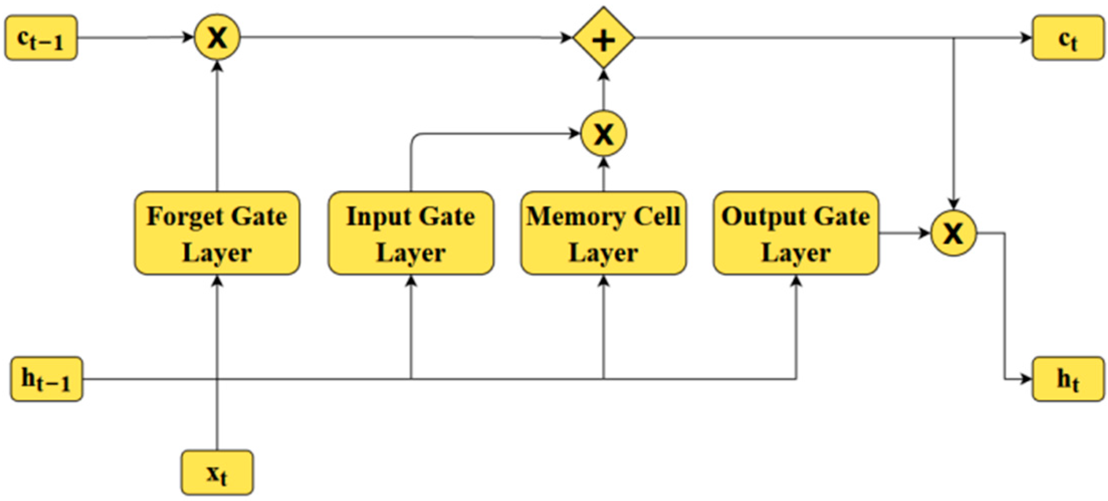
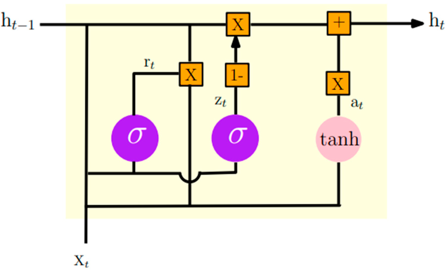
Long Short-Term Memory can predict short-term dependencies by learning the long-term dependencies. It does this with the help of its three gates, i.e., forget gate, input gate, and output gate. The forget gate chooses which information to retain and which to forget. Information from the previous state h(t-1) and input x(t) is passed through an activation function, which generates f(t) as an output for the forget gate.
In the input gate, input x(t) and previous hidden state h(t-1) are passed through activation and through the memory cell layer separately. Their outputs are then used in point-to-point multiplication, which will be used in the next cell state c(t).
The cell state is the combination of the previous cell state c(t-1) and the output of the input gate. Its value is the passed into output gate which decides the next hidden state h(t), which will be forwarded to the next node [56]. Graphically, it is presented below:
Figure A1.
LSTM structure [56].
Figure A1.
LSTM structure [56].

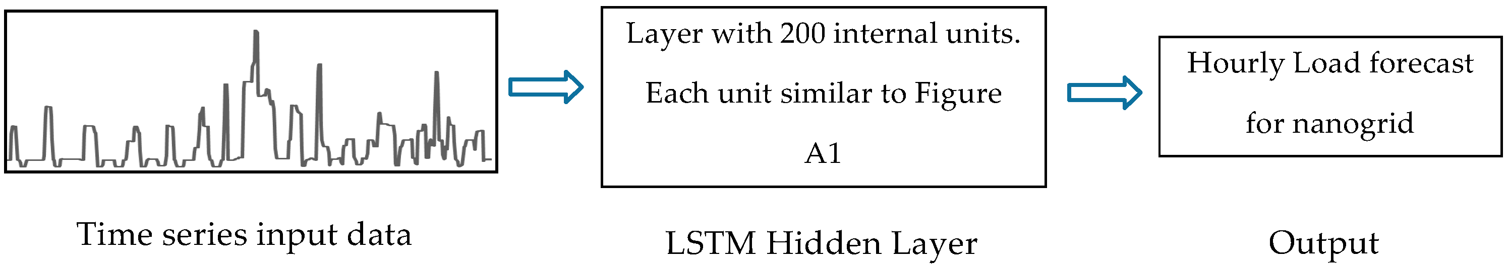
Figure A2 shows the LSTM model that has been used in this paper for comparison with the ANN-based model.
Figure A2.
LSTM model.

Appendix A.2. GRU
GRU belongs to the family of RNN and is very similar in structure and operation to LSTM. Unlike LSTM which has three gates, GRU has two gates, i.e., reset and update. The reset gate associates previous information and the current state while the update gate determines the extent to which information is retained in the current state [57]. In comparison to LSTM, GRU uses lesser information and trains faster. It can be represented graphically in Figure A3.
Figure A3.
The basic structure of GRU [57].
Figure A3.
The basic structure of GRU [57].

Mathematically, GRU operations are formulated in the below equations [57].
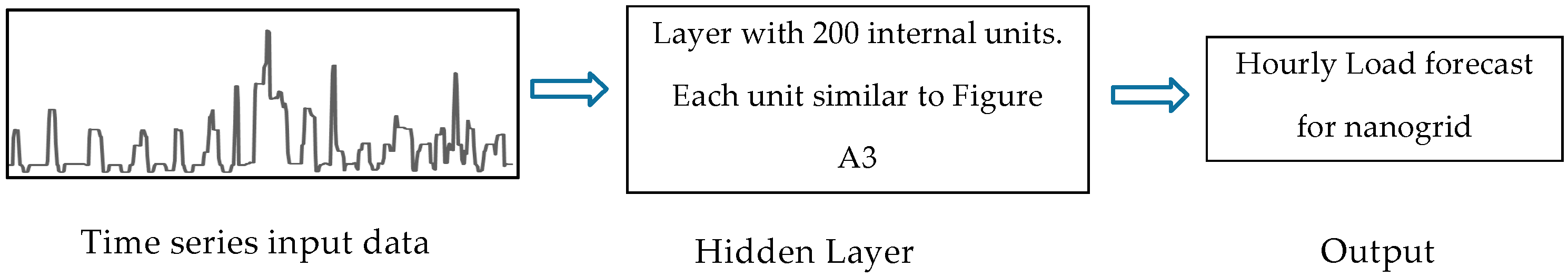
where is the input at time instance t, is the updtae gate, is the reset gate at time t, and represents the output. Figure A4 is the summarized picture of GRU model that is implemented in this paper.
Figure A4.
LSTM model.

Appendix A.3. Bi-LSTM
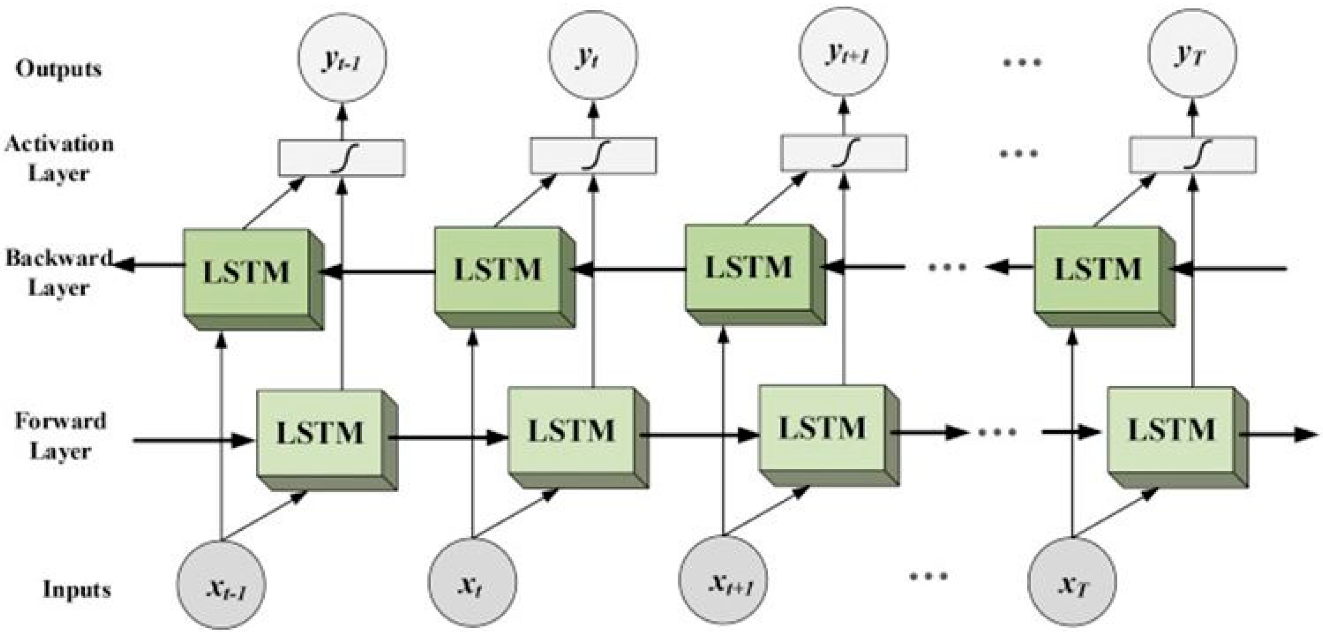
LSTM has only a one-way flow of input (forward or backward) but in Bi-LSTM input is both backward and forwards. This is performed by providing the input to one LSTM (forward) and then the same input is provided in reverse order (Backward) to another LSTM. Outputs of both LSTMs are combined to make a consolidated output [58]. Graphically, it can be represented as Figure A3, obtained from [59].
Figure A5.
The basic structure of Bi-LSTM.

For Bi-LSTM, GRU’s hidden layer is replaced with Bi-LSTM’s hidden layer. Except for this, every parameter will be same as shown in Figure A4.
Appendix B
LSTM, GRU, and Bi-LSTM have been modeled with one hidden layer and 200 internal nodes. The learning rate is set to be 0.001 with exponential decay of gradient. Each model takes an electric load as time series and predicts the hour ahead load of nanogrid. For ease of comparison, the outputs of these models have been evaluated with MAPE, MSE, and CV as performed for the ANN-based model. If results are not satisfactory, hyperparameters are changed and the models are trained again for a fair comparison with our approach ANN. Moreover, these methods have high training times; therefore, their training times are also noted for comparison with ANN. This is because this paper deals with hourly load prediction; therefore, a quicker method is preferred which can forecast within some minutes. In summary, not only the statistical parameters but training time play a major role in determining the superior of the model.
Appendix C
Below is the pseudo-code for LSTM, GRU, and Bi-LSTM models. The same time-series data and parameters have been used for all models; therefore, the below pseudo-code applies to all three.
| Algorithm A1: Pseudo-code for LSTM/GRU/Bi-LSTM Models | |
| Input: Electric load time series | |
| Output: Hourly forecasted electric load and daily energy cost savings | |
| 1. | Get Electric load data |
| 2. | Pre-process the data by converting electric data into hourly electric data |
| 3. | Divide data (Input feature and electric load) into training and testing sets |
| 4. | Initialize LSTM/GRU/Bi-LSTM model |
| 5. | Training time starts |
| 6. | while (1) |
| 7. | Run the model |
| 8. | Losses are calculated |
| 9. | Tune the hyperparameters if needed |
| 10. | if1(Losses(t)-Losses(t-1)< ε) |
| 11. | count = count + 1 |
| 12. | if2 (count > β) |
| 13. | Break |
| 14. | end if2 |
| 15. | end if1 |
| 16. | end while |
| 17. | Training time stops and total training time is calculated (time) |
| 18. | Model tested on test data for hourly load forecasting (Lhour) |
| 19. | MAPE, MSE, CV, and RMSE are calculated |
References
- Burmester, D.; Rayudu, R.; Seah, W.; Akinyele, D. A review of nanogrid topologies and technologies. Renew. Sustain. Energy Rev. 2017, 67, 760–775. [Google Scholar] [CrossRef]
- Yerasimou, Y.; Kynigos, M.; Efthymiou, V.; Georghiou, G. Design of a Smart Nanogrid for Increasing Energy Efficiency of Buildings. Energies 2021, 14, 3683. [Google Scholar] [CrossRef]
- Burgio, A.; Menniti, D.; Sorrentino, N.; Pinnarelli, A.; Motta, M. A compact nanogrid for home ap-plications with a behaviour-tree-based central controller. Appl. Energy 2018, 225, 14–26. [Google Scholar] [CrossRef]
- El-Shahat, A. Nanogrid Technology Increasing, Supplementing Microgrids. Nat. Gas Electr. 2016, 33, 1–7. [Google Scholar] [CrossRef]
- Ahmad, A.; Javaid, N.; Mateen, A.; Awais, M.; Khan, Z.A. Short-Term Load Forecasting in Smart Grids: An Intelligent Mod-ular Approach. Energies 2019, 12, 164. [Google Scholar] [CrossRef]
- Caro, E.; Juan, J.; Cara, J. Periodically correlated models for short-term electricity load forecasting. Appl. Math. Comput. 2019, 364, 124642. [Google Scholar] [CrossRef]
- Huang, Q.; Zheng, Y.; Xu, Y. Microgrid Load Forecasting Based on Improved Long Short-Term Memory Net-work. J. Electr. Comput. Eng. 2022, 2022, 4017708. [Google Scholar]
- Soman, A.; Trivedi, A.; Irwin, D.; Kosanovic, B.; McDaniel, B.; Shenoy, P. Peak Forecasting for Bat-tery-based Energy Optimizations in Campus Microgrids. In Proceedings of the Eleventh ACM International Conference on Future Energy Systems (e-Energy ‘20), Virtual Event, Australia, 22–26 June 2020; ACM: New York, NY, USA, 2010. [Google Scholar]
- Zuleta-Elles, I.; Bautista-Lopez, A.; Catano-Valderrama, M.J.; Marin, L.G.; Jimenez-Estevez, G.; Mendoza-Araya, P. Load Forecasting for Different Prediction Horizons using ANN and ARIMA models. In Proceedings of the 2021 IEEE CHILEAN Conference on Electrical, Electronics Engineering, Information and Communication Technologies (CHILECON), Valparaíso, Chile, 6–9 December 2021; pp. 1–7. [Google Scholar] [CrossRef]
- Arvanitidis, A.I.; Bargiotas, D.; Daskalopulu, A.; Laitsos, V.M.; Tsoukalas, L.H. Enhanced Short-Term Load Forecasting Using Artificial Neural Networks. Energies 2021, 14, 7788. [Google Scholar] [CrossRef]
- Ungureanu, S.; Topa, V.; Cziker, A.C. Deep Learning for Short-Term Load Forecasting—Industrial Consumer Case Study. Appl. Sci. 2021, 11, 10126. [Google Scholar] [CrossRef]
- Marzooghi, H.; Emami, K.; Wolfs, P.J.; Holcombe, B. Short-term Electric Load Forecasting in Microgrids: Issues and Challenges. In Proceedings of the 2018 Australasian Universities Power Engineering Conference (AUPEC), Auckland, New Zealand, 27–30 November 2018; pp. 1–6. [Google Scholar] [CrossRef]
- Kong, W.; Dong, Z.Y.; Jia, Y.; Hill, D.J.; Xu, Y.; Zhang, Y. Short-Term Residential Load Forecasting Based on LSTM Recur-rent Neural Network. IEEE Trans. Smart Grid 2019, 10, 841–851. [Google Scholar] [CrossRef]
- Identifying Potential Markets for Behind-the-Meter Battery Energy Storage: A Survey of U.S. Demand Charges. Available online: https://www.nrel.gov/docs/fy17osti/68963.pdf (accessed on 30 June 2022).
- Rouzbahani, H.M.; Rahimnejad, A.; Karimipour, H. Smart Households Demand Response Management with Micro Grid. In Proceedings of the IEEE Power & Energy Society Innovative Smart Grid Technologies Conference, Washington, DC, USA, 18–21 February 2019; pp. 1–5. [Google Scholar]
- Uddin, M.; Romlie, M.F.; Abdullah, M.F.; Abd Halim, S.; Kwang, T.C. A review on peak load shaving strategies. Renew. Sustain. Energy Rev. 2018, 82, 3323–3332. [Google Scholar] [CrossRef]
- Rana, M.M.; Romlie, M.F.; Abdullah, M.F.; Uddin, M.; Sarkar, M.R. A novel peak load shav-ing algrithm for isolated microgrid using hybrid PV-BESS system. Energy 2021, 234, 121157. [Google Scholar] [CrossRef]
- Abdelsalam, A.A.; Zedan, H.A.; Eldesouky, A.A. Energy Management of Microgrids Using Load Shifting and Multi-agent System. J. Control. Autom. Electr. Syst. 2020, 31, 1015–1036. [Google Scholar] [CrossRef]
- Laboratory for Advanced Software Systems. Available online: https://lass.cs.umass.edu/projects/smart/ (accessed on 30 May 2022).
- Kondaiah, V.; Balasubramanian, S.; Sanjeevkumar, P.; Baseem, K. A Review on Short-Term Load Forecasting Models for Mi-cro-grid Application. J. Eng. 2022, 2022, 665–689. [Google Scholar] [CrossRef]
- Vivas, E.; Allende-Cid, H.; Salas, R. A Systematic Review of Statistical and Machine Learning Methods for Electrical Power Forecasting with Reported MAPE Score. Entropy 2020, 22, 1412. [Google Scholar] [CrossRef]
- Wang, Y.; Zhang, N.; Chen, X. A Short-Term Residential Load Forecasting Model Based on LSTM Recurrent Neural Network Considering Weather Features. Energies 2021, 14, 2737. [Google Scholar] [CrossRef]
- Singh, S.; Hussain, S.; Bazaz, M.A. Short term load forecasting using artificial neural network. In Proceedings of the 2017 Fourth International Conference on Image Information Processing (ICIIP), Shimla, India, 21–23 December 2017; pp. 1–5. [Google Scholar] [CrossRef]
- Chen, Z.; Zhang, D.; Jiang, H.; Wang, L.; Chen, Y.; Xiao, Y.; Liu, J.; Zhang, Y.; Li, M. Load Forecasting Based on LSTM Neural Network and Applicable to Loads of “Re-placement of Coal with Electricity”. J. Electr. Eng. Technol. 2021, 16, 2333–2342. [Google Scholar] [CrossRef]
- Tayab, U.B.; Zia, A.; Yang, F.; Lu, J.; Kashif, M. Short-term load forecasting for microgrid energy management system using hybrid HHO-FNN model with best-basis stationary wavelet packet transform. Energy 2020, 203, 117857. [Google Scholar] [CrossRef]
- Moradzadeh, A.; Zakeri, S.; Shoaran, M.; Mohammadi-Ivatloo, B.; Mohammadi, F. Short-Term Load Forecasting of Microgrid via Hybrid Support Vector Regression and Long Short-Term Memory Algorithms. Sustainability 2020, 12, 7076. [Google Scholar] [CrossRef]
- Quilumba, F.L.; Lee, W.-J.; Huang, H.; Wang, D.Y.; Szabados, R.L. Using Smart Meter Data to Improve the Accuracy of Intra-day Load Forecasting Considering Customer Behavior Similarities. IEEE Trans. Smart Grid 2015, 6, 911–918. [Google Scholar] [CrossRef]
- Lee, G.-C. Regression-Based Methods for Daily Peak Load Forecasting in South Korea. Sustainability 2022, 14, 3984. [Google Scholar] [CrossRef]
- Caliano, M.; Buonanno, A.; Graditi, G.; Pontecorvo, A.; Sforza, G.; Valenti, M. Consumption based-only load forecasting for individual households in nanogrids: A case study. In Proceedings of the 2020 AEIT International Annual Conference (AEIT), Catania, Italy, 23–25 September 2020. [Google Scholar] [CrossRef]
- Dong, H.; Gao, Y.; Fang, Y.; Liu, M.; Kong, Y. The Short-Term Load Forecasting for Special Days Based on Bagged Regression Trees in Qingdao, China. Comput. Intell. Neurosci. 2021, 2021, 3693294. [Google Scholar] [CrossRef] [PubMed]
- Kelo, S.; Dudul, S. A wavelet Elman neural network for short-term electrical load prediction under the influence of tempera-ture. Int. J. Electr. Power Energy Syst. 2012, 43, 1063–1071. [Google Scholar] [CrossRef]
- Khwaja, A.S.; Zhang, X.; Anpalagan, A.; Venkatesh, B. Boosted neural networks for improved short-term electric load fore-casting. Electr. Power Syst. Res. 2017, 143, 431–437. [Google Scholar] [CrossRef]
- Borghini, E.; Giannetti, C.; Flynn, J.; Todeschini, G. Data-Driven Energy Storage Scheduling to Minimise Peak Demand on Distribution Systems with PV Generation. Energies 2021, 14, 3453. [Google Scholar] [CrossRef]
- Szczepanik, W.; Niemiec, M. Heuristic Intrusion Detection Based on Traffic Flow Statistical Analysis. Energies 2022, 15, 3951. [Google Scholar] [CrossRef]
- Vairagade, N.; Logofatu, D.; Leon, F.; Muharemi, F. Demand Forecasting Using Random Forest and Artificial Neural Network for Supply Chain Management. In Computational Collective Intelligence, Proceedings of the 11th International Conference, ICCCI 2019, Hendaye, France, 4–6 September 2019; Lecture Notes in Computer Science; Springer: Cham, Switzerland, 2019; pp. 328–339. [Google Scholar] [CrossRef]
- Rahul, G.K.; Singh, S.; Dubey, S. Weather Forecasting Using Artificial Neural Networks. In Proceedings of the 2020 8th International Conference on Reliability, Infocom Technologies and Optimization (Trends and Future Directions) (ICRITO), Noida, India, 4–5 June 2020; pp. 21–26. [Google Scholar] [CrossRef]
- Tran, T.; Bateni, S.; Ki, S.; Vosoughifar, H. A Review of Neural Networks for Air Temperature Forecasting. Water 2021, 13, 1294. [Google Scholar] [CrossRef]
- Radicioni, M.; Lucaferri, V.; De Lia, F.; Laudani, A.; Presti, R.L.; Lozito, G.; Fulginei, F.R.; Schioppo, R.; Tucci, M. Power Forecasting of a Photovoltaic Plant Located in ENEA Casaccia Research Center. Energies 2021, 14, 707. [Google Scholar] [CrossRef]
- Elsheikh, A.H.; Muthuramalingam, T.; Shanmugan, S.; Ibrahim, A.M.M.; Ramesh, B.; Khoshaim, A.B.; Moustafa, E.B.; Bedairi, B.; Panchal, H.; Sathyamurthy, R. Fine-tuned artificial intelligence model using pigeon optimizer for prediction of residual stresses during turning of Inconel 718. J. Mater. Res. Technol. 2021, 15, 3622–3634. [Google Scholar] [CrossRef]
- Moustafa, E.B.; Hammad, A.H.; Elsheikh, A.H. A new optimized artificial neural network model to predict thermal efficiency and water yield of tubular solar still. Case Stud. Therm. Eng. 2021, 30, 101750. [Google Scholar] [CrossRef]
- Elsheikh, A.H.; Panchal, H.; Ahmadein, M.; Mosleh, A.O.; Sadasivuni, K.K.; Alsaleh, N.A. Productivity forecasting of solar distiller integrated with evacuated tubes and external condenser using artificial intelligence model and moth-flame optimizer. Case Stud. Therm. Eng. 2021, 28, 101671. [Google Scholar] [CrossRef]
- Lizhen, W.; Yifan, Z.; Gang, W.; Xiaohong, H. A novel short-term load forecasting method based on mini-batch stochastic gradient descent regression model. Electr. Power Syst. Res. 2022, 211, 108226. [Google Scholar] [CrossRef]
- Phyo, P.-P.; Jeenanunta, C. Advanced ML-Based Ensemble and Deep Learning Models for Short-Term Load Forecasting: Comparative Analysis Using Feature Engineering. Appl. Sci. 2022, 12, 4882. [Google Scholar] [CrossRef]
- Kim, D.-H.; Lee, E.-K.; Qureshi, N. Peak-Load Forecasting for Small Industries: A Machine Learning Approach. Sustainability 2020, 12, 6539. [Google Scholar] [CrossRef]
- Hodo, E.; Bellekens, X.; Iorkyase, E.; Hamilton, A.; Tachtatzis, C.; Atkinson, R. Machine Learning Approach for Detection of nonTor Traffic. In Proceedings of the 12th International Conference on Availability, Reliability and Security, Reggio Calabria, Italy, 29 August–1 September 2017; p. 85. [Google Scholar] [CrossRef] [Green Version]
- Aponte, O.; McConky, K. Peak electric load days forecasting for energy cost reduction with and without behind the meter renewable electricity generation. Int. J. Energy Res. 2021, 45, 18735–18753. [Google Scholar] [CrossRef]
- Hernandez, L.; Baladrón, C.; Aguiar, J.M.; Carro, B.; Sanchez-Esguevillas, A.J.; Lloret, J. Short-Term Load Forecasting for Microgrids Based on Artificial Neural Networks. Energies 2013, 6, 1385–1408. [Google Scholar] [CrossRef]
- Li, R.; Sun, F.; Ding, X.; Han, Y.; Liu, Y.P.; Yan, J.R. Ultra short-term load forecasting for user-level integrated energy system considering multi-energy spatio-temporal coupling. Power Syst. Technol. 2020, 44, 4121–4134. [Google Scholar]
- Zhu, R.; Guo, W.; Gong, X. Short-Term Load Forecasting for CCHP Systems Considering the Correlation between Heating, Gas and Electrical Loads Based on Deep Learning. Energies 2019, 12, 3308. [Google Scholar] [CrossRef]
- Zheng, J.; Zhang, L.; Chen, J.; Wu, G.; Ni, S.; Hu, Z.; Weng, C.; Chen, Z. Multiple-Load Forecasting for Integrated Energy System Based on Copula-DBiLSTM. Energies 2021, 14, 2188. [Google Scholar] [CrossRef]
- Activation Functions. Available online: https://paperswithcode.com/methods/category/activation-functions (accessed on 25 June 2022).
- Publication Ready NN-Architecture Schematics. Available online: https://alexlenail.me/NN-SVG/ (accessed on 20 August 2022).
- Elsheikh, A.H.; Sharshir, S.W.; Elaziz, M.A.; Kabeel, A.; Guilan, W.; Haiou, Z. Modeling of solar energy systems using artificial neural network: A comprehensive review. Sol. Energy 2019, 180, 622–639. [Google Scholar] [CrossRef]
- Azeem, A.; Ismail, I.; Jameel, S.M.; Romlie, F.; Danyaro, K.U.; Shukla, S. Deterioration of Electrical Load Forecasting Models in a Smart Grid Environment. Sensors 2022, 22, 4363. [Google Scholar] [CrossRef] [PubMed]
- Greater Boston Rates. Available online: https://www.eversource.com/content/docs/default-source/rates-tariffs/ema-greater-boston-rates.pdf (accessed on 30 June 2022).
- Shohan, M.J.A.; Faruque, M.O.; Foo, S.Y. Forecasting of Electric Load Using a Hybrid LSTM-Neural Prophet Model. Energies 2022, 15, 2158. [Google Scholar] [CrossRef]
- Mahjoub, S.; Chrifi-Alaoui, L.; Marhic, B.; Delahoche, L. Predicting Energy Consumption Using LSTM, Multi-Layer GRU and Drop-GRU Neural Networks. Sensors 2022, 22, 4062. [Google Scholar] [CrossRef] [PubMed]
- Petrosanu, D.-M.; Pîrjan, A. Electricity Consumption Forecasting Based on a Bidirectional Long-ShortTerm Memory Artificial Neural Network. Sustainability 2021, 13, 104. [Google Scholar] [CrossRef]
- Complete guide to Bi-Directional LSTM (With Python Codes). Available online: https://analyticsindiamag.com/complete-guide-to-bidirectional-lstm-with-python-codes/ (accessed on 30 August 2022).
Figure 1.
Schematics of nanogrid and microgrid.

Figure 2.
Thresholding of correlation co-efficient using K-means.

Figure 3.
Basic structure of ANN neuron [38].
Figure 3.
Basic structure of ANN neuron [38].

Figure 4.
ANN network [52].
Figure 4.
ANN network [52].

Figure 5.
Schematics of the developed methodology.

Figure 6.
Decomposition of nanogrid load (01/01/2016 to 01/15/2016).

Figure 7.
Correlation map of input features and electric load.

Figure 8.
Scatter Plot ANN, LSTM, GRU, and Bi-LSTM models.

Figure 9.
Violin Plot for each model.

Figure 10.
Taylor diagram for ANN, LSTM, GRU, and Bi-LSTM models.

Figure 11.
Load Forecasting for an extreme summer week.

Figure 12.
Load Forecasting for an extreme winter week.


Table 1.
STLF algorithms and their implementation for micro-grid and the grid.
| Paper Title | Classification | Algorithm | Summary/Results | Area |
|---|---|---|---|---|
| [6] A novel hybrid forecasting scheme for electricity demand time series’ | Statistical | ARIMA | Spain’s grid load forecasting has been performed while incorporating non-linear effects of temperature and special days for hourly 1 to 10 days ahead demand. | Grid |
| [28] Regression-Based Methods for Daily Peak Load Forecasting in South Korea | Statistical | ARIMA | Implementation of ARIMA in a South Korean grid showed a MAPE of 1.95%. | Grid |
| [7] Microgrid Load Forecasting Based on Improved Long Short-Term Memory Network | ML | LSTM | The model has been implemented for a micro-grid utilizing 5 years of load data. Results show improvement by reduction of MAPE from 8% to within 4%. | Microgrid |
| [10] Enhanced Short-Term Load Forecasting Using Artificial Neural Networks | ML | ANN | This work predicts load forecasting for Greek Intercontinental Power System with various scaling methods for input data. Based on the scaling method, MAPE changes from 2.73% to 1.76%. | Grid |
| [11] Deep Learning for Short-Term Load Forecasting: Industrial Consumer Case Study | ML & Statistical | GRU, ARIMA, LSTM, RNN and their combinations | Woodworking factory’s load was predicted using numerous mentioned methods. Amongst these, GRU outperformed others with a MAPE of 4.82%. Exogenous and lagged load data were used as input features. | Factory (Microgrid) |
| [29] Short and mid-term load forecasting using machine learning models | ML & Statistical | LR, SVR, GBRT | New York Independent System Operators (NYISO) dataset was used for the implementation of these algorithms and a comparison, on basis of MAPE, was drawn. Previous load and meteorological data were used as input features. It was found that the hybrid model AdaBoost and GBRT showed improved results with the MAPE of 2.27%. | Grid |
| [9] Load Forecasting for Different Prediction Horizons using ANN and ARIMA models | ML & Statistical | ANN & ARIMA | Microgrid load has been trained using ANN and compared with ARIMA. ANN captures more random behavior which is corroborated by the results: ANN is 0.5% more accurate than ARIMA in day-ahead prediction and 3.5% more accurate in an hour-ahead prediction. | Microgrid |
Table 2.
Parameters for ANN, LSTM, GRU and Bi-LSTM models.
| Parameters | ANN | LSTM | GRU | BI-LSTM |
|---|---|---|---|---|
| Input Features | Meteorological and electrical load features | Electric load time series | Electric load time series | Electric load time series |
| Output | Hourly load forecast | Hourly load forecast | Hourly load forecast | Hourly load forecast |
| Number of hidden layers | 3 | 1 | 1 | 1 |
| Number of neurons in 1st hidden layer | 30 | - | - | - |
| Number of neurons in 2nd hidden layer | 30 | - | - | - |
| Number of neurons in 3rd hidden layer | 20 | - | - | - |
| Number of internal nodes | - | 200 | 200 | 200 |
| Learning Rate | 0.0001 | 0.001 | 0.001 | 0.001 |
| Internal Optimizer | Adam | Adam | Adam | Adam |
| Epoch | 300 | 10 | 10 | 10 |
| Activation Function | ReLu | ReLu | ReLu | ReLu |
| Batch Size | 32 | 32 | 32 | 32 |
| Regularization | l-1 on 3rd hidden layer | - | - | - |
| Weight Initialization | Random | Random | Random | Random |
Table 3.
Simulation results for hour-ahead load forecasting of a nanogrid.
| Evaluation Parameters | ANN | LSTM | GRU | Bi-Directional LSTM |
|---|---|---|---|---|
| MSE (KW) | 0.03 | 0.37 | 0.34 | 0.35 |
| RMSE (KW) | 0.17 | 0.60 | 0.55 | 0.59 |
| MAPE (%) | 9.00 | 28.0 | 26.1 | 25.0 |
| CV (%) | 11.9 | 33.7 | 32.3 | 32.8 |
| Training Time (min) | 7.50 | 39.40 | 27.6 | 38.7 |
Table 4.
Peak load identification and energy cost saving in a nanogrid.
| Date | Hour Indices for Peak Load | Daily Energy Cost without Peak Shifting ($) | Daily Energy Cost with Peak Shifting ($) | Energy Cost Saving (%) |
|---|---|---|---|---|
| 2016 August 20 | 4:00 PM | 0.28 | 0.22 | 21.0% |
| 2016 August 21 | 12:00 PM | 0.77 | 0.58 | 24.3% |
| 2016 August 22 | 6:00 PM | 0.12 | 0.09 | 24.3% |
| 2016 August 23 | 2:00 PM, 3:00 PM, 4:00 PM, 5:00 PM, 9:00 PM | 0.51 | 0.41 | 19.2% |
| 2016 August 24 | 3:00 PM, 4:00 PM, 5:00 PM, 6:00 PM, 7:00 PM | 1.08 | 0.81 | 24.3% |
| 2016 August 25 | 2:00 PM, 3:00 PM, 5:00 PM | 0.75 | 0.56 | 25.0% |
| 2016 August 26 | 3:00 PM, 4:00 PM, 6:00 PM | 0.33 | 0.26 | 20.9% |
Table 5.
Weekly energy cost savings in nanogrid through peak shifting.
| Week | Weekly Energy Cost without Peak Shifting ($) | Weekly Energy Cost with Peak Shifting ($) | Cost Saving (%) | |
|---|---|---|---|---|
| Extreme Summer | 2016 July 15 to 2016 July 21 | 6.03 | 5.02 | 16.7 |
| Extreme Winter | 2016 February 1 to 2016 August 1 | 28.4 | 25.9 | 8.85 |
Publisher’s Note: MDPI stays neutral with regard to jurisdictional claims in published maps and institutional affiliations. |
© 2022 by the authors. Licensee MDPI, Basel, Switzerland. This article is an open access article distributed under the terms and conditions of the Creative Commons Attribution (CC BY) license (https://creativecommons.org/licenses/by/4.0/).
Share and Cite
MDPI and ACS Style
Kumar, A.; Yan, B.; Bilton, A. Machine Learning-Based Load Forecasting for Nanogrid Peak Load Cost Reduction. Energies 2022, 15, 6721. https://doi.org/10.3390/en15186721
AMA Style
Kumar A, Yan B, Bilton A. Machine Learning-Based Load Forecasting for Nanogrid Peak Load Cost Reduction. Energies. 2022; 15(18):6721. https://doi.org/10.3390/en15186721
Chicago/Turabian StyleKumar, Akash, Bing Yan, and Ace Bilton. 2022. "Machine Learning-Based Load Forecasting for Nanogrid Peak Load Cost Reduction" Energies 15, no. 18: 6721. https://doi.org/10.3390/en15186721
Note that from the first issue of 2016, this journal uses article numbers instead of page numbers. See further details here.