Electrochemical Impedance Spectroscopy Based on the State of Health Estimation for Lithium-Ion Batteries

Highlights

• EIS was used to estimate the SOH of LIBs found to be fast and effective.
• It is more convenient to use CNN to extract features of EIS data automatically.
• The improved ECM method and IPSO-CNN-BiLSTM method are proposed in this paper.
• IPSO algorithm was first proposed to applied to the problem of optimizing the initial parameters of the neural networks.

Abstract

The state of health (SOH) is critical to the efficient and reliable use of lithium-ion batteries (LIBs). Recently, the SOH estimation method based on electrochemical impedance spectroscopy (EIS) has been proven effective. In response to different practical applications, two models for SOH estimation are proposed in this paper. Aiming at based on the equivalent circuit model (ECM) method, a variety of ECMs are proposed. Used EIS to predict the ECM, the results show that the improved method ensures the correctness of the ECM and improves the estimation results of SOH. Aiming at a data-driven algorithm, proposes a convolution neural network (CNN) to process EIS data which can not only extract the key points but also simplifies the complexity of manual feature extraction. The bidirectional long short-term memory (BiLSTM) model was used for serial regression prediction. Moreover, the improved Particle Swarm Optimization (IPSO) algorithm is proposed to optimize the model. Comparing the improved model (IPSO-CNN-BiLSTM) with the traditional PSO-CNN-BiLSTM, CNN-BiLSTM and LSTM models, the prediction results are improved by 13.6%, 93.75% and 94.8%, respectively. Besides that, the two proposed methods are 27% and 35% better than the existing gaussion process regression (GPR) model, which indicates that the proposed improved methods are more flexible for SOH estimation with higher precision.

1. Introduction

With the development and consummation of electric vehicles, information systems and energy storage systems, LIBs are being used more and more widely because of their advantages (high energy density and low cost) [1,2]; moreover, the scale of LIBs is also increasing with the continuous expanding of application scenarios [3]. Estimating the SOH of LIBs during the aging process, can improve safety and prolong service life [4,5].

Due to the interaction of various degradation mechanisms in the aging process of LIBs, it is a significant and challenging issue to detect the SOH of LIBs rapidly and effectively. SOH is an indicator used to compare the current performance of a battery with a brand new battery [2,6]. The deterioration of battery aging is usually accompanied by capacity attenuation, energy density decrease, voltage difference increase when charging and discharging and so on [7]. The standard definition of the SOH has not been finally unified, capacity is typically defined in the literature:

$$\mathrm{SOH}=\frac{C_{now-}{C}_{eol}}{C_{new-}{C}_{eol}}\times 100\%$$

(1)

where $C_{now}$ is the current capacity of a used battery, $C_{eol}$ is end of life capacity (usually 80% of $C_{new}$) of the representative battery, and $C_{new}$ is the capacity of a brand-new battery.

At present, the estimation method mainly based on voltage, current and temperature obtained by battery management system (BMS) [8]. With the constant cycle of battery charging and discharging, irreversible changes will occur inside the cell (lithium dendrite and SEI layer growth, electrolyte reduction, etc.) [9]; this will lead to a decrease in the available battery capacity (SOH) [10]. It will also cause an increase in voltage difference and temperature in the process of charging and discharging. Monitoring the voltage, current, and temperature of LIBs to estimate SOH is based on this principle [11,12]. However, the efficiency of this method is greatly reduced due to the indirect way. A kind of effective method is the use of ultrasonic nondestructive testing technology to obtain the components and chemical states (electrodes, residual electrolytes) of LIBs directly (

Table 1. Non-destructive testing technology (NDT technology).

Measurement Technique	Specific Method
Based on X-ray techniques	(1) X-ray Diffraction (XRD) (2) Energy Dispersive Spectroscopy (EDS) (3) X-ray Absorption Spectroscopy (XAS) (4) X-ray Photoelectron Technique (XPT)
Electron and Scanning probe microscopy	(1) Scanning Electron Microscopy (SEM) (2) Transmission Electron Microscopy (TEM) (3) Electron Probe Microscopic Analysis (EPMA) (4) Focused Ion Beam (FIB)
Spectroscopic techniques	(1) Fourier Transform InfraRed spectrometry (FTIR) (2) Raman spectroscopy (3) Prompt Gamma Activation Analysis (PGAA)

). Although this method can accurately show the degradation mechanism inside the LIB, cannot automatically identify the SOH. Relate the SOH with the internal state of LIBs (lithium dendrite growth degree, SEI layer thickness) detected by ultrasonic nondestructive testing will be the direction in the future [13,14].

Recently, EIS, has been developed to estimate the SOH of LIBs; moreover, it has been proved that the prediction accuracy is higher than that of the traditional voltage, current and temperature data [15]. EIS is a new diagnostic technique and has the advantage of non-destructive. During the tests, wide frequency is applied to LIB to reflect the cell’s EIS information (imaginable part, real part, and phase Angle) at different temperatures and SOC. The changes of cathode, anode, electrolyte and solid electrolyte layer (SEI) can be adequately reflected in the aging process of LIBs. The EIS technique compared with traditional BMS, and nondestructive testing technology has the advantages of fast detection speed and rich reflection information [16,17]. EIS is usually measured by voltage excitation or current excitation. The voltage excitation type is measured by applying a sinusoidal voltage of a certain frequency range to the cell and analyze the output current and phase. However, this method requires constant voltage during the measurement process, which is not conducive to online measurement. Therefore, measuring by current excitation be the mode usually adopt.

2. Gap Analysis and Original Contributions

There are two main methods for estimating SOH by EIS[18], which are based on ECM method and deep learning method (Table 2). The principle of based on the ECM method is to fit the EIS measured at different temperatures and SOC states with the ECM [19,20,21]. It is possible to obtain the parameters of the ECM, necessary to reconstruct the discharge curves of the LIBs, to study their cycling performance and to understand if they have anomalous ageing during operation. Besides, some parameters vary with the ageing of the LIBs and can be used to determine the SOH. Xiong Rui et al. established the relationship with SOH by fitting SEI resistors in the ECM [22]. Matteo Galeotti et al. used the ohmic resistance to estimate the SOH [23]. However, the above two methods do not consider the influence of temperature and SOC in the process of testing. A model considers synchronously the two factors was proposed by Xueyuan Wang et al. [24]:

$$R_{ct}=\frac{{\alpha }_{1}Texp\left(\frac{{\alpha }_2}{T}\right)}{\sqrt{SO{C}^2+{\beta }_{1}SOC+{\beta }_2}}$$

(2)

${\alpha }_1$, ${\alpha }_2$, ${\beta }_1$ and ${\beta }_2$ are parameters that need to be determined, and $T$ represents the temperature of LIBs. The model can predict $R_{ct}$ at any temperature and SOC, making the EIS technology more flexible and accurate to characterize the aging status of LIBs. On this basis, the mapping between $R_{ct}$ and SOH was set up by Qunming Zhang et al. [25]. The precision of ECM influence the estimation accuracy of SOH directly. However, the proposed method only considers one ECM in circuit fitting, which is prone to the problem of poor fitting accuracy due to an inaccurate model. Aiming at such problem, a new method of predicting ECMs by EIS is proposed in this article. To find the ECM with the highest fitting accuracy, which can fundamentally improve the accuracy and robustness of the prediction model [26,27].

Since the data-driven methods of process monitoring rely only on the historic process data and do not assume any form of model information, they have been paid more attention [28,29,30]. The SOH prediction of LIBs using machine learning methods usually requires a large amount of historical data for preprocessing [31,32,33]. It takes the SOH as the output of the model, the features with high correlation were extracted as the input of the machine learning model [34,35]. The modeling results show high accuracy based on the model adaptive iteration of the data. Yunwei Zhang et al. using GPR method, real and imaginary parts of impedance with frequency range from 0.02–20,000 Hz were used as model input. The SOH and remaining useful life (RUL) of LIBs were accurately predicted [36,37]. On this basis, different features were extracted by Chun Chang et al. and using Elman neural network and cuckoo search (CS-Elman) model to estimate the SOH [3]. Besides, neural network models such as deep Neural network(DNN) and recurrent Neural networks (RNNs) have also been proved to be effective in estimating SOH [38]. However, all the above methods require manual data processing for the EIS in advance, which is often practically unfeasible in many applications. T. K. Pradyumna et al. proposed a CNN model, the eigenvalues with high correlation between SOH and EIS are automatically extracted as the input; this reduces the chance of leaving out important features from the data, which can happen in the case of manual feature extraction; moreover, also can reduce the calculation complexity greatly. However, the performance is slow with simple CNN when dealing with regression problems. Combining CNN with other regression prediction models will be the next study emphasis.

The method based on ECM and data-driven method were combined is a new research direction, the parameters of the fitted circuit are regarded as input parameters of the neural network. Yige Li et al. proposed a method to predict the parameters of ECM using the Artificial Neural Network (ANN) model [39]. The ohmic resistance, SEI resistor and charge-transfer resistance as the inputs of the BP neural network to estimate SOH [40]. Marvin Messing et al. using the combining method to estimate SOH, the results indicated that has worse accuracy than the traditional single method. The reason is that the combination of the two methods not only increases the amount of calculation but also increases the error. Improving the accuracy and robustness of the estimation model will be beneficial to the present research [41].

Table 2. Typical studies on predicting SOH based on EIS.

Researchers	Calculation Basis	Description
Xiong Rui et al. [42]	Based on model method	Establish the relationship between $R_{sei}$ and the SOH
Matteo Galeotti et al. [23]	Based on model method	Establish the relationship between ohmic resistance and the SOH
Xueyuan Wang et al. [24]	Based on model method	Establish the relationship between $R_{ct}$, T and SOC
Qunming Zhang et al. [25]	Based on model method	Establish the relationship between $R_{ct}$ and SOH
Yunwei Zhang et al. [36]	Based on data-driven method	Built the EIS and GPR model
Chun Chang et al. [15]	Based on data-driven method	Built the EIS and CS-Elman model
Marvin Messing et al. [38]	Based on data-driven method	Built the EIS and DNN model
Akram Eddahech et al. [43]	Based on data-driven method	Built the EIS and RNNs model
T. K. Pradyumna et al. [44]	Based on data-driven method	Built the EIS and CNN model
Yige Li et al. [39]	Based on model and data-driven method	Used ANN to predict the equivalent circuit parameters
Chao Lyu et al. [40]	Based on model and data-driven method	Input $R_{ct}$, $R_{sei}$ to the BP neural network

Table 2. Typical studies on predicting SOH based on EIS.

Researchers	Calculation Basis	Description
Xiong Rui et al. [42]	Based on model method	Establish the relationship between $R_{sei}$ and the SOH
Matteo Galeotti et al. [23]	Based on model method	Establish the relationship between ohmic resistance and the SOH
Xueyuan Wang et al. [24]	Based on model method	Establish the relationship between $R_{ct}$, T and SOC
Qunming Zhang et al. [25]	Based on model method	Establish the relationship between $R_{ct}$ and SOH
Yunwei Zhang et al. [36]	Based on data-driven method	Built the EIS and GPR model
Chun Chang et al. [15]	Based on data-driven method	Built the EIS and CS-Elman model
Marvin Messing et al. [38]	Based on data-driven method	Built the EIS and DNN model
Akram Eddahech et al. [43]	Based on data-driven method	Built the EIS and RNNs model
T. K. Pradyumna et al. [44]	Based on data-driven method	Built the EIS and CNN model
Yige Li et al. [39]	Based on model and data-driven method	Used ANN to predict the equivalent circuit parameters
Chao Lyu et al. [40]	Based on model and data-driven method	Input $R_{ct}$, $R_{sei}$ to the BP neural network

Aiming at the shortages of the methods based on ECM and the data-driven methods, two improvement methods are proposed. Overall, the novel contributions of this paper are as follows:

(1)

A method based on multi-ECMs is presented with the consideration of ambient temperature effect. By using the least square method, EIS data are used to predict the ECM. The changing trends and aging mechanism of each circuit parameter with SOH decay were analyzed. Both mechanism analysis and experimental study set the foundation for EIS-based SOH estimation. The parameter with the highest correlation were extracted. As far as we know, none of the existing work has quantitatively studied the EIS-based SOH estimation by multiple equivalent circuit models.

(2)

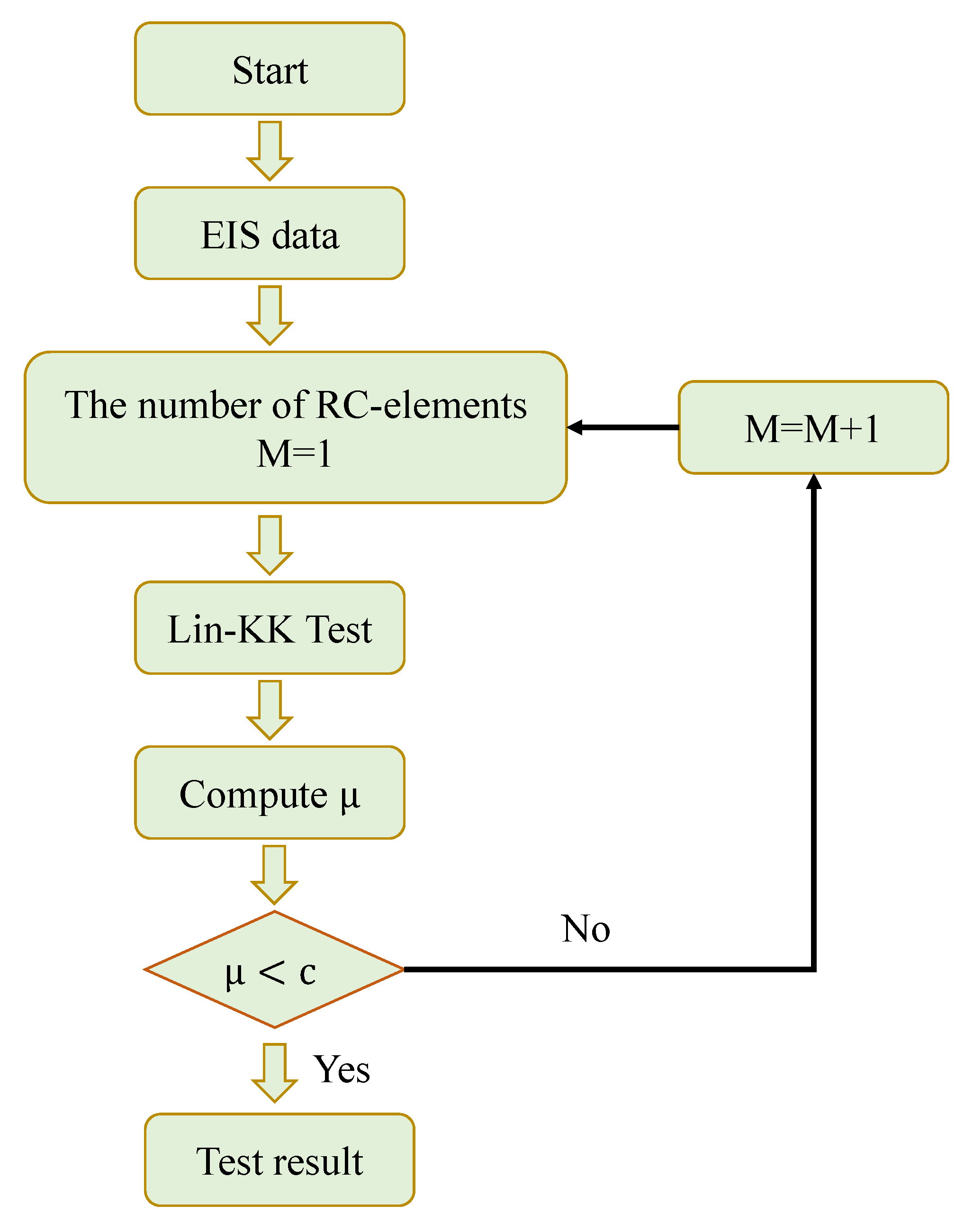
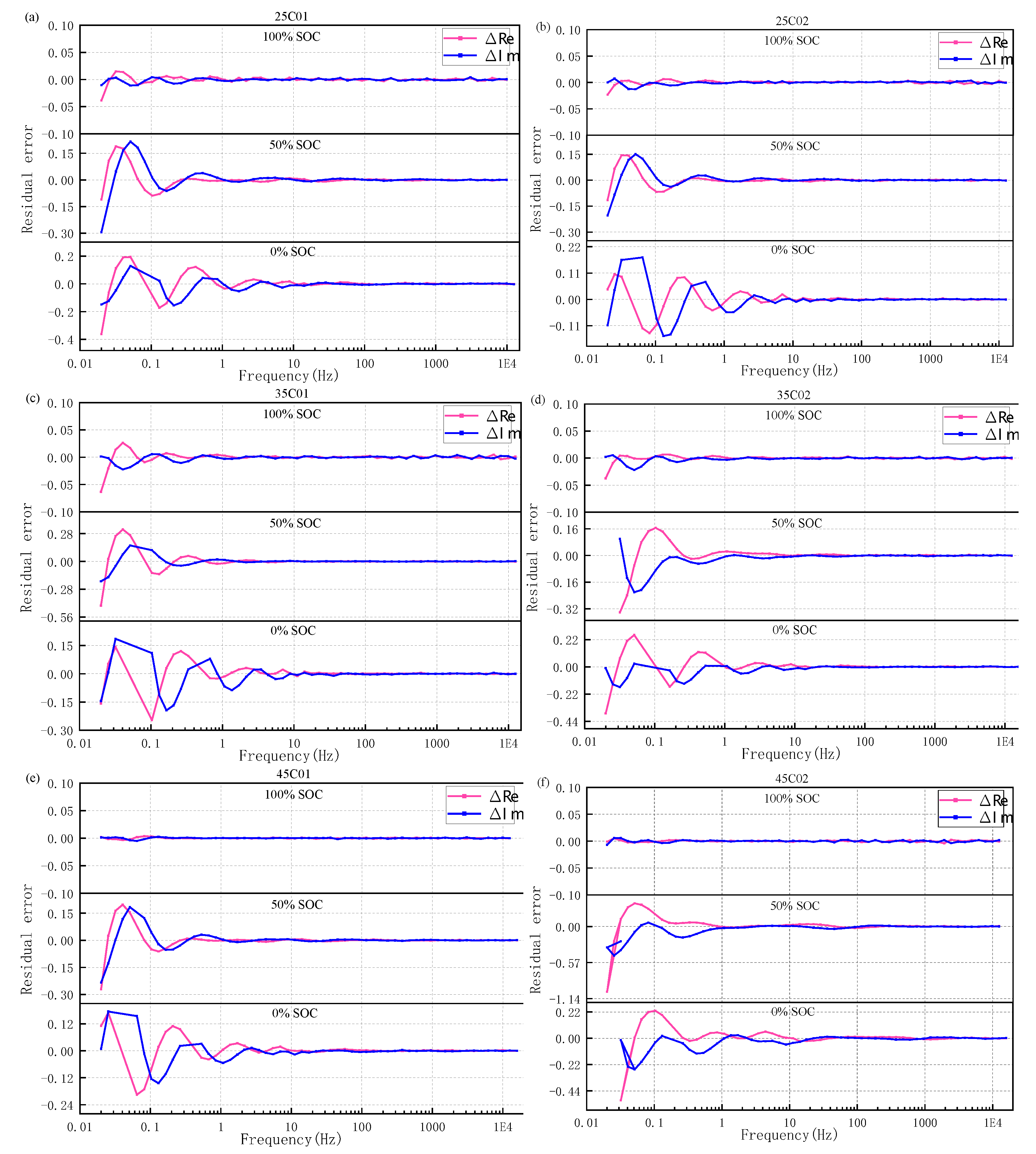
The EIS data used in some current studies are directly derived from electrochemical workstations. However, operational errors, effects of the conductor or other unexpected accident, may result in damage of EIS data. Kramers-Kronig (K-K) relations were used to verify the reliability of the EIS data.

(3)

A new method (CNN) is put forward, which can implement auto-extracting of EIS data. Greatly reduce the complexity of manual data processing. It makes feature extraction more convenient and reduces the chance of leaving out important features from the data.

(4)

The EIS is collected between charging and discharging cycles, which are time series, the recurrent neural network (RNN) is suitable to process time series when making use of internal memory. Compared with Simple RNN, BiLSTM has the advantages of adequately prevent gradients exploding and gradient vanishing. By coupling CNN with BiLSTM neural network, a regression model is established, which can enhance the forecast precision effectively and maintain robustness.

(5)

Owing to the large number of parameters in the CNN-BiLSTM model which requires a lot of tweaking for the ideal precision. PSO algorithm is adopted to optimize parameters of CNN-BiLSTM. The constriction factor PSO algorithm is easily trapped in the local optimum and appeared premature convergence. The number of hidden layer nodes, learning rate of neural network are optimized using an improved particle swarm optimization (IPSO) algorithm. Learning quality and training speed of the neural network are improved. The validity and accuracy of modeling are tested by simulations, and the simulation results of the comparison between other neural networks and the model’s identification are given.

(6)

Different methods for estimating SOH are compared and improvement models is presented. It is a major task to be settled.

Article Organisation

The remainder of this paper is organized as follows. Section 3 introduces cell aging and EIS data validation. Section 4 multi-models the LIBs and identifies the ECM parameters. Present the SOH estimation method based on EIS and verifications and discussions. Section 5 presents the IPSO-CNN-BiLSTM model and verifications with different temperature and neural network models. Different methods’ estimation results of SOH are discussed in Section 6. Section 7 is the conclusion and outlook of this paper.

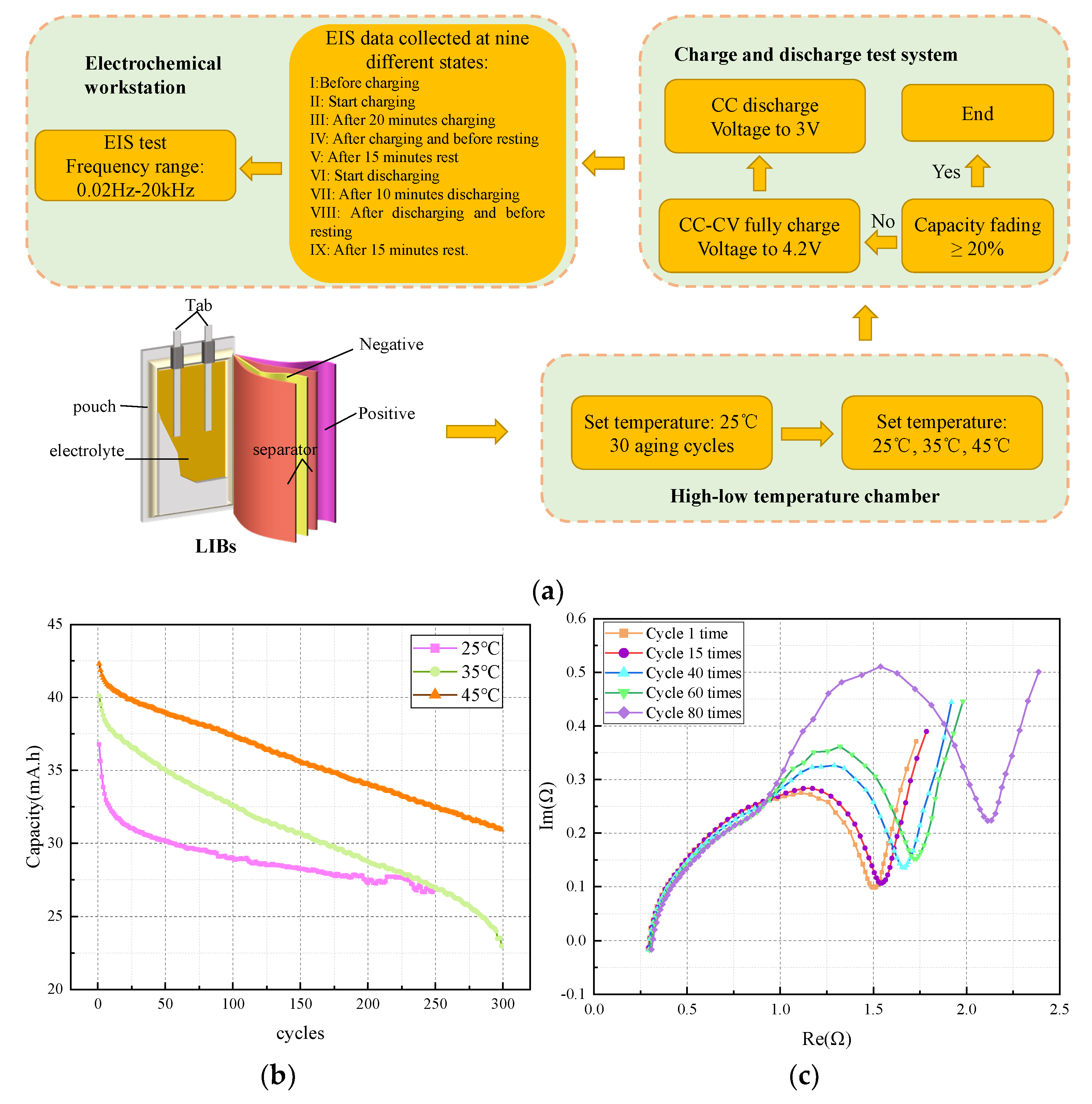
3. Battery Aging and EIS Data Validation

3.1. Battery Aging

Twelve Eunicell LR2032 LIBs with a capacity of 45 mAh were subjected to aging experiments until the cell’s capacity faded to its designed capacity (80% of the initial capacity) by Yunwei Zhang et al. [36]. Considering the different operating temperatures of LIBs, the aging of each LIB is tested in different ambient temperatures (25 °C, 35 °C, 45 °C). Eight of the LIBs were placed at 25 °C and numbered 25C01–25C08, respectively. There two LIBs were placed at 35 °C, numbered 35C01–35C02, respectively; moreover, the other LIBs were placed at 45 °C, numbered 45C01–45C02, respectively. Each cycle consists of a 1C–rate (45 mA) CC–CV (constant current–constant voltage) charge up to 4.2 V and a 2C–rate (90 mA) CC (constant current) discharge down to 3 V. EIS is measured at nine different stages of charging/discharging during every even-numbered cycle in the frequency range of 0.02 Hz–20 kHz with an excitation current of 5 mA. In order to determine the rated capacity of each LIB, 30 charge–discharge cycles had been studied at 25 °C before it was placed at a different ambient temperature. Therefore, we erase the data of the first 30 times when processing EIS data. The capacity decay curve, as well as EIS test process of LIBs as Figure 1.

3.2. EIS Data Validation

Over 20,000 EIS spectra of commercial LIBs are collected at different SOH, state of charge (SOC) and temperatures—the largest dataset to our knowledge of its kind. However, in the process of EIS testing, the applied AC current, range of frequency sweep, points per decade represented, length of the pause time after a change in the SOC and length of the pause time after a change in the ambient temperature et al. all have affect to obtain useful results from EIS tests [45]. In order to estimate SOH, requires the measured spectrum to be a representation of a linear, time-invariant and causal system. A valid EIS data should conform to the K-K relations [46,47]. The relevant equations:

$$Z_{Re}\left(\omega \right)=\frac{2}{\pi }{{\displaystyle \int }}_0^{\infty }\frac{{\omega }^{\prime }{Z}_{Im}\left({\omega }^{\prime }\right)}{{\omega }^2-{\omega }^{\prime 2}}\mathrm{d}{\omega }^{\prime }$$

(3)

$$Z_{Im}\left(\omega \right)=\frac{-2}{\pi }{{\displaystyle \int }}_0^{\infty }\frac{{\omega }^{\prime }{Z}_{Re}\left({\omega }^{\prime }\right)}{{\omega }^2-{\omega }^{\prime 2}}\mathrm{d}{\omega }^{\prime }$$

(4)

By applying Equations (4) or (5) to either the real part or imaginary part of a measured spectrum, the remaining part can be computed. By comparing the latter to the according measured part, the spectrum’s accordance to the K-K relations can be judged. However, the arising problem of missing parts of the impedance when approaching frequencies of zero and infinity can’t be avoided. A Lin-KK approach that overcame this was introduced by M. Schönleber et al.: Instead of directly evaluating Equations (4) and (5), the accordance of an impedance spectrum with the K-K relations is judged by its reproducibility by an appropriate K-K compliant ECM. A series connection RC-elements general model is chosen, where the resistors as well as the time-constants of the ECM are fitted to a measured EIS. The error value between the fitted impedance and the actual data are used to determine whether the data conform to the K-K relationship. The ECM to be fitted to measured impedance spectra as shown in Figure 2.

The ECM impedance expression is given by:

$$\hat{\mathrm{Z}}\left(\omega \right)={\widehat{R}}_{ohm}+{\displaystyle \sum }_{k=1}^M\frac{{\widehat{R}}_k}{1+j\omega {\tau }_k}$$

(5)

where, the distribution of the time constants is responsible to the angular frequency of the impedance. The smallest time-constant (${\tau }_{min}$) is given by:

$${\tau }_{min}={\tau }_1=\frac{1}{{\omega }_{max}}$$

(6)

So, the largest time-constant (${\tau }_{max}$) is given by:

$${\tau }_{max}={\tau }_M=\frac{1}{{\omega }_{min}}$$

(7)

The time-constants ${\tau }_k$ are distributed logarithmically equal over the inverse range of angular frequencies of the EIS to be tested. All other time-constants are therefore given by:

$${\tau }_k={10}^{\left[\log \left({\tau }_{min}\right)+\frac{k-1}{M-1}\ast \log \left(\frac{{\tau }_{max}}{{\tau }_{min}}\right)\right]} \left(k=2,\dots \dots ,M-1\right)$$

(8)

In order to judge the reproducibility of a measured EIS data by the fitted ECM, a measure describing an according deviation, the residual, is described as:

$${\mathsf{\Delta }}_{Re}\left(\omega \right)=\frac{Z_{Re}\left(\omega \right)-{\hat{\mathrm{Z}}}_{Re}\left(\omega \right)}{\left|Z\left(\omega \right)\right|}$$

(9)

or

$${\mathsf{\Delta }}_{Im}\left(\omega \right)=\frac{Z_{Im}\left(\omega \right)-{\hat{\mathrm{Z}}}_{Im}\left(\omega \right)}{\left|Z\left(\omega \right)\right|}$$

(10)

The number of RC-elements have higher requirements during the Lin-KK test. If the selected numbers are less, that the order of the ECM is too small to fit the measured EIS, the residuals will large, even though the latter might in fact be fully compliant with the K-K relations. On the other hand, if the selected number of RC-elements is too large, not only the useful information contained in the EIS is fitted, but the measurement noise as well. Hence, the according residuals will also indicate invalidity, even though the tested EIS is fully valid. It’s worth noting that between the noise part and the information part of an EIS is the fact that neither the real part nor the imaginary part of an ideal spectrum shows oscillatory behavior when plotted over the frequency. Therefore, all oscillations contained in a measured EIS data are caused by noise or measurement errors. On the other hand, a fitted spectrum that oscillates cannot be physically valid and must have been tuned to noise or other errors, which is again precisely the definition of overfitting; moreover, oscillations can only occur if some of the ohmic resistance have a negative sign. In order to prevent the fit from oscillating the influence of negatively signed ohmic elements has to be limited. To quantify this index, a measure relating the mass of negatively signed elements to the mass of the positively signed elements is proposed by:

$$\mathsf{\mu }=1-\frac{{{\displaystyle \sum }}_{{\mathrm{R}}_{\mathrm{k}}<0}\left|{\mathrm{R}}_{\mathrm{k}}\right|}{{{\displaystyle \sum }}_{{\mathrm{R}}_{\mathrm{k}}\ge 0}\left|{\mathrm{R}}_{\mathrm{k}}\right|}$$

(11)

where the value of $\mathsf{\mu }$ is between zero and 1, as soon as over-fitting starts, the mass of negative elements increases and $\mathsf{\mu }$ monotonously goes to zero. By judging the magnitude of $\mathsf{\mu }$ in the fitting process to confirm the number of RC-elements (Figure 3).

The value of $\mathrm{c}$ is a design parameter, however from the previous study’s experience $\mathrm{c}$ = 0.85 has proven to be an excellent choice.

Using the Lin-KK method, the EIS data of six LIBs (25C01, 25C02, 35C01, 35C02, 45C01, 45C02) at different temperatures and SOC until the end-of-life cycle were tested. The fitting residual results are shown in Figure 4.

As can be seen in Figure 4, the residual is larger at low frequencies at the state of 0% SOC and 50% SOC. However, the residuals are much smaller at the state of 100% SOC. In addition, the average fitting residuals of each LIBs are shown in

Table 3. Lin–KK test mean residual (mean values of fitted residuals for EIS data at all cycles of LIBs).

LIBs	SOC	$\left|{\mathsf{\Delta }}_{\mathit{R}\mathit{e}}\right|$	$\left|{\mathsf{\Delta }}_{\mathit{I}\mathit{m}}\right|$
25C01	0%	0.004232971	0.016325792
	50%	0.003294959	0.006302259
	100%	0.000140785	0.001371033
25C02	0%	0.001918329	0.010518637
	50%	0.001635152	0.0037642
	100%	8.25 × 10−5	0.000912258
35C01	0%	0.006345962	0.016388624
	50%	0.007214271	0.011049813
	100%	0.000186722	0.001439418
35C02	0%	0.004387341	0.015948539
	50%	0.003831015	0.004872054
	100%	0.000137274	0.001328463
45C01	0%	0.002577748	0.009078397
	50%	0.0026469	0.005081625
	100%	6.30 × 10−6	0.000107301
45C02	0%	0.005054565	0.01810478
	50%	0.006414285	0.014348096
	100%	3.73 × 10−5	0.000319163

. As can be seen from the table, the results of the mean fitting error are consistent with the fitting error of the impedance data at a single cycle. The fitting residuals will be different under different SOC states. The closer the SOC is to 100%, the lower of fitting residuals data, which indicates that the EIS more conform to the K–K relationships. Although at different temperatures, the residuals in the same SOC state less variations within the acceptable range; this indicates that whether EIS conforms to the K–K relationship is only related to the SOC of LIB itself and has nothing to do with the ambient temperature. However, even for different LIBs at the same temperature and SOC, the mean residual will be different. Such as 25C01 and 25C02 average real part ($\left|{\mathsf{\Delta }}_{Re}\right|$) residuals are 0.00014, 8.25 × 10⁻⁵ respectively. It is chiefly because the impedance of different LIB will also change due to different internal changes and external interference during the charging and discharging process. However, beyond that, no matter $\left|{\mathsf{\Delta }}_{Im}\right|$ or $\left|{\mathsf{\Delta }}_{Re}\right|$, which are just not the same deriving. The former uses the known real part data to calculate the imaginary part, while the latter is the reverse. Both can be used to determine whether the EIS data conforms to the K–K relationship.

Above all, it indicates that the EIS data at 100% SOC are more consistent with the K−K relationship. Therefore, in order to avoid the effect on the SOH prediction accuracy of LIBs due to the error of EIS data itself. EIS data under 100% SOC were adopted as training features.

4. Based on Improved Equivalent Circuit Model Method

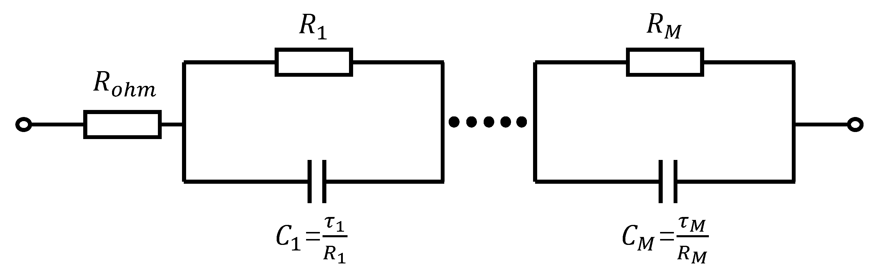
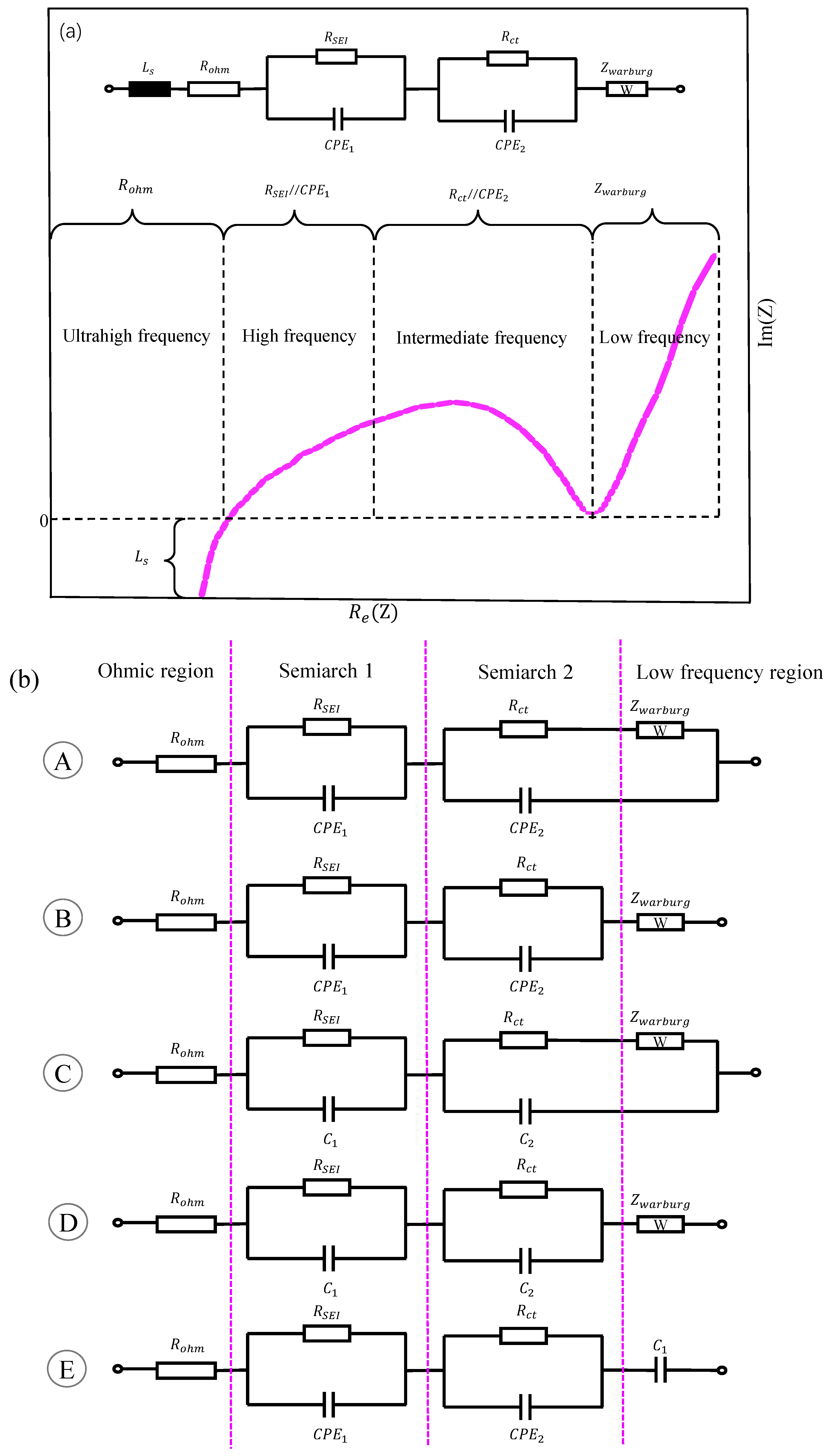
4.1. ECM of LIBs

The physical effects that occur in any electrochemical system can be associated to the electrical parameters of an ECM, useful to quantify the phenomena that occur inside the LIBs during charging, discharging and ageing processes. The internal process of LIBs during the cycle aging can be quantified by the electrical parameters. The relationship between general ECM and EIS is established and in Figure 5a.

The ultrahigh frequency segment, a vertical line below the real axis, is the inductive effects caused by the movement of electrons in the wire and the winding of internal electrodes, which is represented by an inductor $L_s$. The intersection of the vertical line and the X-axis is the ohmic resistance formed by the movement of electrons in the solid phase metal and ions in the electrolyte phase, which is represented by $R_{ohm}$. The high frequency segment is the first arc produced by the diffusion of lithium ions through the SEI film. A constant phase element (instead of ideal capacitors), $CP{E}_1$, is introduced to describe the film capacitance considering the dispersion effect and $R_{SEI}$ represents the SEI resistance. Where, the impedance expression of $CP{E}_1//R_{SEI}$ is:

$$Z_{CP{E}_1//R_{SEI}}=\frac{R_{SEI}}{1+R_{SEI}{C}_{PE1}{\left(j\omega \right)}^{{\alpha }_1}}$$

(12)

where ${\alpha }_1$ at the denominator of the expressions denotes an angle that rotates in the complex plane relative to a pure capacity behavior. If ${\alpha }_1=1$, the impedance is a pure capacitor, if ${\alpha }_1=0$, the result is a pure resistance. The intermediate frequency segment is the second arc that describes the charge transfer process in electrode reaction. Another constant phase element $CP{E}_2$ is used to describe the double-layer capacitance. The low frequency segment is the diffusion tail.

There is no definite for ECM of LIBs. Using EIS to estimate the ECM can be a good solution to this problem. With the aging of the LIBs, its internal structure may change, the ECM will also change accordingly. Five different ECMs were proposed to adapt to the variations, which have been verified to have good accuracy. It analyzes different models for fitting the EIS data by comparing their precision. In order to ensure the veracity of ECM, adopted ECM with the highest fitting accuracy (Figure 5b).

(1)

ECM (a) is modelled by exploiting two-time constants (parallel $CPE//\mathrm{R}$) for the intermediate frequency region. The Warburg element is placed on the resistive branch of the second $CPE//\mathrm{R}$ element to describe the diffusive behavior of the LIBs and also fit the low frequency tail of the impedance curve. A warburg element is used to reproduce the diffusion phenomena of the ions in the electrolyte during the discharging and charging processes. The impedance expression of the element can be expressed as:

$$Z_{\mathrm{W}}=\frac{1}{C_{PEW}{\left(j\omega \right)}^{{\alpha }_w}}$$

(13)

(2)

Two-time constants (parallel $CPE//\mathrm{R}$) are used by ECM (b) to separate the intermediate frequency region and the Warburg element is placed in series with respect to the other circuital elements. The two-time constants respectively to describe SEI layer for anode-cell and the cathode electrolyte interface (CEI) layer for the cathode-cell.

(3)

ECM (c) modelled by exploiting RC elements for the intermediate frequency region, which is the only difference with ECM (a). The cathode ECM instead includes a modified RC element with a Warburg element in the capacitive branch; this choice allowed to a better description of the cathode EIS spectrum.

(4)

ECM (d) is a modified Randles model: an RC element is used to model the surface layer process; a second RC element is used to model charge transfer and double layer effects and a Warburg element in parallel to a capacitance is used to model the low frequency tail.

(5)

The ECM (e) presents an identical configuration to ECM (b), using C elements instead of Warburg to describe the diffusive behavior.

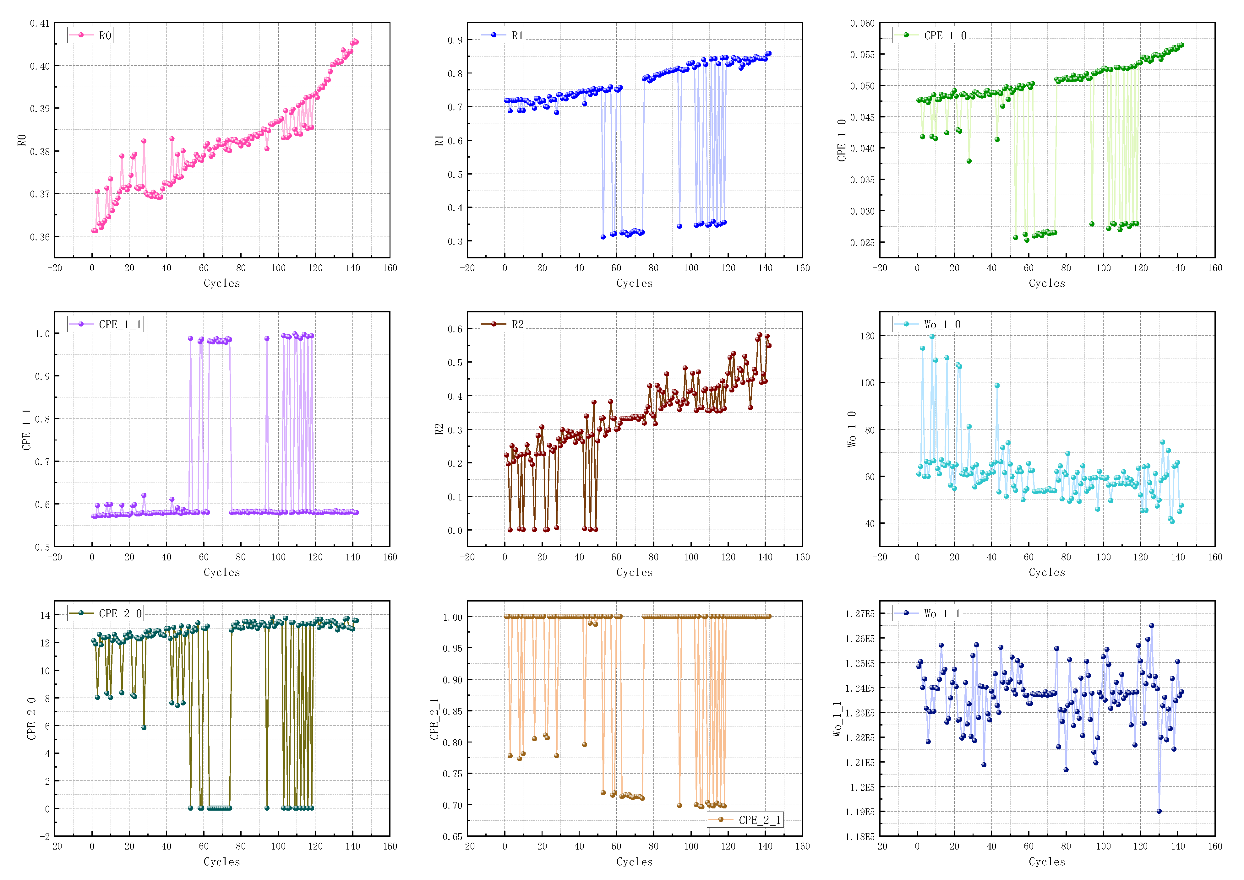
4.2. ECM Fitting

The fitting of ECM is performed by non-linear least squares regression of the circuit model to impedance data via curve fit from the scipy.optimize package. Real and imaginary components are fit simultaneously with uniform weighting, i.e., the objective function to minimize is:

$${\chi }^2={\displaystyle \sum }_{n=0}^N{\left[Z_{data}^{\prime }\left({\omega }_n\right)-Z_{model}^{\prime }\left({\omega }_n\right)\right]}^2+{\left[Z_{data}^{″}\left({\omega }_n\right)-Z_{model}^{″}\left({\omega }_n\right)\right]}^2$$

(14)

where $N$ is the number of frequencies and $Z^{\prime }$ and $Z^{″}$ are the real and imaginary components of the impedance, respectively.

By default, the high dimensionality of typical ECM. Basinhopping optimization algorithms used to attempt to search the entire parameter landscape to minimize the error. The fitting results of different ECM are as follows:

Where, the expression of RMSE is:

$$\mathrm{RMSE}=\sqrt{\frac{{{\displaystyle \sum }}_{i=1}^N{\left(Z_{\mathrm{fit}\left(\mathrm{i}\right)}-Z_{data\left(i\right)}\right)}^2}{N}}$$

(15)

As seen in

Table 4. The root mean square error (RMSE) of LIBs under different ECMs.

LIBs	ECM (a)	ECM (b)	ECM (c)	ECM (d)	ECM (e)
25C01	0.020008042	0.05372	0.02826916	0.028172482	0.023061876
25C02	0.026388823	0.012999786	0.034571499	0.035265693	0.026932343
35C01	0.016677489	0.032265334	0.02020132	0.022164251	0.023895306
35C02	0.016722439	0.014605039	0.018846951	0.018415463	0.024565196
45C01	0.015605166	0.014130575	0.016370651	0.016421256	0.021315892
45C02	0.012373409	0.013167452	0.013819581	0.034023868	0.022499835

, the fitting RMSE of ECM (a) and ECM (b) is relatively low than the other three models. However, the fitting error of ECM(b) fluctuates greatly. In this paper, the ECM (a) is used for SOH estimation. By taking 25C01 as an example, the parameters variation trend of ECM (a) components is shown in Figure 6:

The degradation of lithium-ion batteries is caused by many physical and chemical mechanisms, including different degradation mechanisms. There are three common degradation modes: the loss of lithium inventory, anodic active material loss and the loss of cathodic active material [48]. Due to the parasitic reactions, decomposition reactions (SEI layer decomposition, electrolyte decomposition), SEI layer growth, resulting in lithium-ion consumption [49]. Insufficient to support the cycle between cathode and anode, resulting in capacity fade. Structural disordering, particle cracking, graphite exfoliation, loss of electrical contact or blocking of the active sites, which can lead to the decline of active anode materials; this will also cause the battery capacity fade. Similarly, these damages will also occur at the cathode and cause the loss of cathode active material. At present, a large number of studies have described the most sensitive phenomenon of capacity loss in LIBs as the growth of SEI resistance and ohmic resistance. The growth of SEI resistance is mainly characterized by the impedance rise in the intermediate frequency region [50]. The growth of ohmic resistance is due to the decomposition of electrolyte during battery aging [51,52]. In addition, the cathode charge transfer velocity decreases during the aging process [53]. However, the change in the latter is less pronounced than in the first two; these conclusions are consistent with our experimental results.

With the aging of LIBs, the trend of $R_0$ (ohmic resistance) and $R_1$(SEI resistor) become big gradually. Because the capacity fade of LIB is principally due to the growth of an SEI layer on anode side of the battery during cycling, that results in an increase in the $R_{ohm}$ and a loss of capacity at the same time. Considering that much noise is generated when the $R_1$ increasing, $R_0$ is finally used as a feature index to estimate SOH.

4.3. SOH Estimation Model

The relationship between SOH and $R_0$ follows:

$$\mathrm{SOH}\left(R_0\right)=a_1\times \exp \left(-{\left(\frac{R_0-b_1}{c_1}\right)}^2\right)$$

(16)

where $a_1$, $b_1$, and $c_1$ are constant parameters.

The above model is used to fit the LIBs data at 25 °C, 35 °C, 45 °C and the results are listed in

Table 5. Model fitting results under different temperature.

Temperature	LIBs	Coefficients (with 95% Confidence Bounds)			RMSE	R-Square
		${\mathit{a}}_1$	${\mathit{b}}_1$	${\mathit{c}}_1$
25 °C	25C01	0.9542 (0.9345, 0.974)	0.3655 (0.3644, 0.3666)	0.02343 (0.02219, 0.02467)	0.0540	0.9678
25 °C	25C02	0.9496 (0.919, 0.9801)	0.2123 (0.2085, 0.2162)	0.05471 (0.05071, 0.05871)	0.0534	0.9071
35 °C	35C01	0.8651 (0.8386, 0.8916)	0.289 (0.2872, 0.2908)	0.02606 (0.02419, 0.02793)	0.0793	0.9227
35 °C	35C02	0.2541 (0.123, 0.3852)	1.698 (1.565, 1.832)	0.1751 (0.06872, 0.2815)	0.0691	0.9453
45 °C	45C01	0.9493 (0.929, 0.9696)	0.01734 (0.01717, 0.0175)	0.003553 (0.003402, 0.003705)	0.0541	0.9661
45 °C	45C02	1.003 (0.9383, 1.067)	0.06305 (0.0621, 0.06401)	0.008891 (0.008181, 0.009602)	0.0497	0.9693

. Accordingly, the SOH model of LIB with different temperatures is reached as:

$$\mathrm{SOH}\left(R_0,T\right)=\left\{\begin{array}{c}0.9542\times \exp \left(-{\left(\frac{R_0-0.3655}{0.02343}\right)}^2\right),T=25 °\mathrm{C}\\ 0.8651\times \exp \left(-{\left(\frac{R_0-0.289}{0.02606}\right)}^2\right),T=35 °\mathrm{C}\\ 0.9493\times \exp \left(-{\left(\frac{R_0-0.01734}{0.003553}\right)}^2\right),T=45 °\mathrm{C}\end{array}\right.$$

(17)

As seen in Table 5, both RMSE and $R^2$ showed acceptable ranges. The validity of the method is demonstrated. The $R^2$ represents the goodness of fit, which value has to be between 0 and 1. The closer that this value is to 1, the more significant goodness-of-fit is. In addition, the improvement model has fewer parameters than other models. Consequently, the estimation speed will improve significantly.

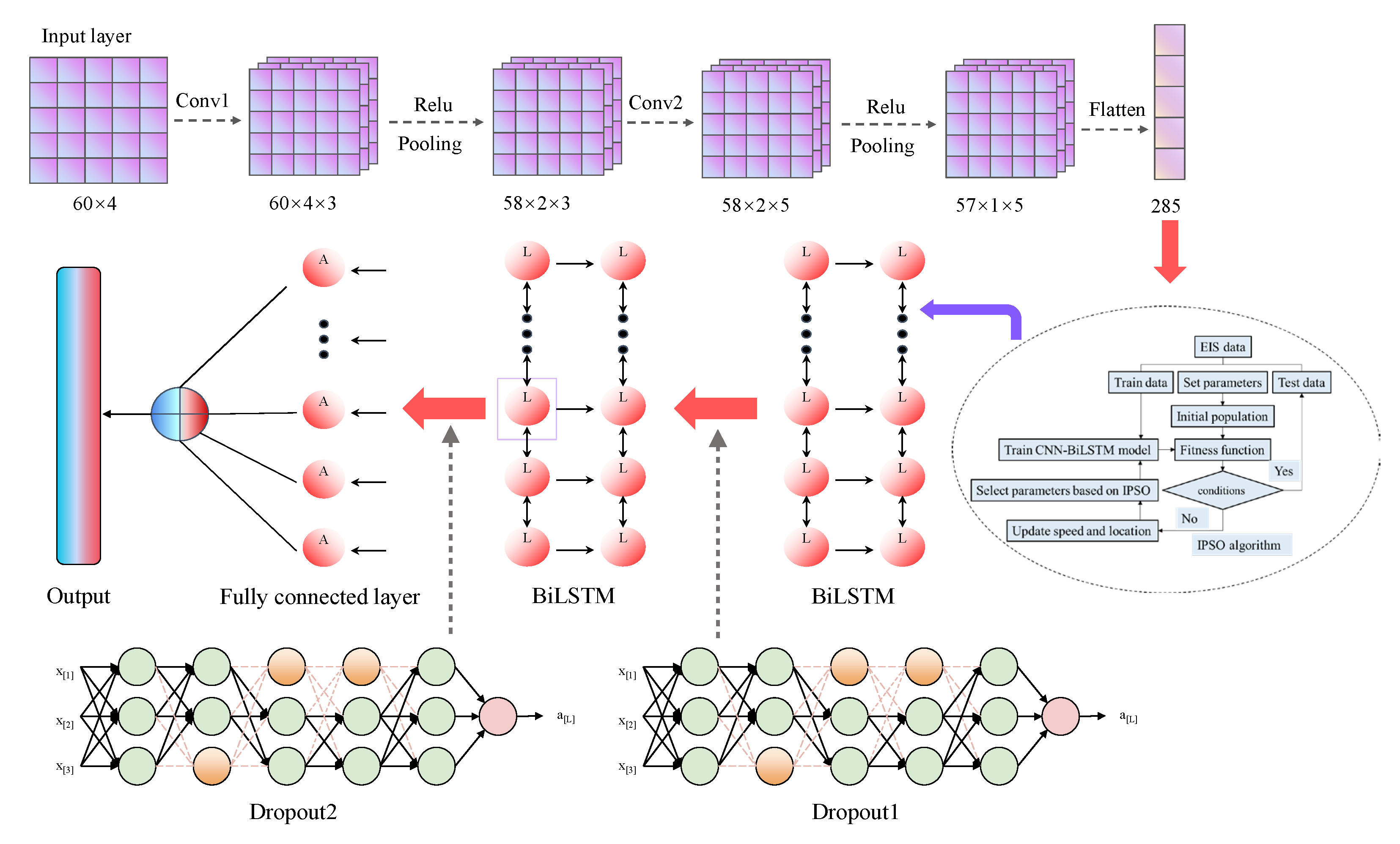
5. Based on the Improved IPSO-CNN-BiLSTM Model Method

5.1. Overview of CNN

The advantage of CNN is able to extract important features from data without any manual interactions. Because of the rich information content contained in EIS data, using CNN greatly reduce the complexity of processing data and ensures that no loss of important information. CNN includes input layer, convolution layer, activation layer and fully connected layer.

The input layer is used to perform preprocessing of the input EIS data, which includes the real part, imaginary part, modulus and phase at 60 different frequencies under each charge/discharge cycle. Normalization was performed firstly, and the formula is:

$$x_{normalization}=\frac{x-x_{Min}}{x_{Max}-x_{Min}}$$

(18)

where, the $x_{Max}$ and $x_{Min}$ is the maximum and minimum value of the sample data respectively. The same impedance plot can be represented in the form of a 60 × 4 shaped arrays with real, imaginary, module and phase values of the impedance after processing.

Filters are used to extract important features in the whole range of input data at the convolution layers. The convolution can be represented by Equation (20).

$$\mathrm{Convoluton} \mathrm{Layer}:\mathsf{\sigma }\left(\mathrm{W}\times \mathrm{x}+\mathrm{b}\right)$$

(19)

The nonlinear mapping on the output results of the convolution layer are implemented in the activation layers. Common excitation functions are as follows:

$$\mathrm{Sigmoid}\left(\mathrm{x}\right)=\frac{1}{1+e^{-x}}$$

(20)

$$\tanh \left(\mathrm{x}\right)=\frac{e^{2x}-1}{e^{2x}+1}$$

(21)

$$\mathrm{Relu}\left(\mathrm{x}\right)=\max \left(0,\mathrm{x}\right)=\left\{\begin{array}{c}0 \left(x\le 0\right)\\ x \left(x\ge 0\right)\end{array}\right.$$

(22)

Due to its quick convergence, find the gradient easily, the activation function of Relu are widely used in various fields. Therefore, the Relu activation function is selected in the excitation layer. The pooling layer sandwiched between different convolution layers, which is used in data compressing. Simulation experiments show that the algorithm can remove the noise and preserve EIS data’s original features effectively. The common method of pooling include max pooling and average pooling. The average pooling is adopted in this paper. The flatten layer is used to convert the two-dimensional image data to one-dimensional digital temporal signals, then input them to the regression neural network model.

In order not to skip important features, adding multiple CNN layers for feature extraction is necessary. The network structure is shown in

Table 6. Details of the CNN architecture.

Designation	Specifications
Input layer	60 × 4
Conv1	3 filters, filter size 2 × 1
Pooling	average pooling, 2 × 2
Conv2	5 filters, filter size 3 × 1
Pooling	average pooling, 3 × 3
Flatten	285

.

5.2. Overview of LSTM

Because the data of the EIS are collected between charging and discharging cycles, which are time series, the recurrent neural network (RNN) is suitable to process time series when making use of internal memory. Because the different neurons of simple RNN hidden layers have contacts. The output of the hidden layer is not merely determined by the current input, it is also about the previous time point; this makes the simple RNN memorizable. However, simple RNN cannot keep long memories because of the gradient explosion and gradient disappearance. The LSTM was created based on the Simple RNN. By adding the memory gating structure to the hidden layers of simple RNN, remembering and forgetting of previous and current information can be controlled and relative application in other field [54,55,56,57]. A new state c was added to the simple RNN to preserve the long-term state. There are three gating units in LSTM: forget gate, input gate and output gate. The previous state c_t−1 of units was entered into the current state c_t, which was controlled by forget gate. The input gate determines how much of the current input x_t goes into the current unit state x_t. The output gate was used to determine the output at the current moment, which combines the current memory and long-term state. The calculation formula for each gate function and state transfer process in the LSTM module is as follows:

$$f_t=\sigma \left(W_f\left[h_{t-1},x_t\right]+b_f\right)$$

(23)

$$i_t=\sigma \left(W_i\left[h_{t-1},x_t\right]+b_i\right)$$

(24)

$${\tilde{c}}_t=tanh\left(W_c\left[h_{t-1},x_t\right]+b_c\right)$$

(25)

$$o_t=\sigma \left(W_o\left[h_{t-1},x_t\right]+b_o\right)$$

(26)

$$c_t=f_t\times c_{t-1}+i_t\times {\tilde{c}}_t$$

(27)

$$h_t=o_t\times \tanh \left(c_t\right)$$

(28)

where, f_t, i_t and o_t are the outputs of forget gate, input gate and output gate respectively. h_t−1 and h_t are the previous value and current value in the network. c_t−1, c_t are the state of the previous and current time respectively. ${\tilde{c}}_t$ is the current memory of the network. W_f, b_f, W_i, b_i, W_o, b_o, W_c, b_c are the weight matrix and bias terms of forget gate, input gate, output gate and computing element, respectively. σ and tanh all are the nonlinear activation function.

The activation functions and derivatives adopted by LSTM are shown in formula 31 to 41:

$$\mathsf{\sigma }\left(\mathrm{z}\right)=\mathrm{y}=\frac{1}{1+{\mathrm{e}}^{-\mathrm{z}}}$$

(29)

$${\mathsf{\sigma }}^{\prime }\left(\mathrm{z}\right)=y\left(1-y\right)$$

(30)

$$tanh\left(z\right)=y=\frac{e^z-e^{-z}}{e^z+e^{-z}}$$

(31)

$${\mathit{tanh}}^{\prime \left(z\right)}=1-y^2$$

(32)

5.3. Overview of Bi-LSTM

Bi-LSTM can synthesize the output in both directions to adjust the weight values. Reading the time series data from both directions, then output the results with a comprehensive balance. The accuracy of training can be improved greatly. Having information between the past and the future for the features, which is the design philosophy of Bi-LSTM. The simulation proves that the performance of Bi-LSTM is better than LSTM. The state of forward and reverse hidden layer as shown in Formula (35) to (36).

$${\overrightarrow{H}}_t=\varphi (X_t{W}_{xh}^{\left(f\right)}+{\overrightarrow{H}}_{t-1}{W}_{hh}^{\left(f\right)}+b_h^{\left(f\right)})$$

(33)

$${\overleftarrow{H}}_t=\varphi (X_t{W}_{xh}^{\left(b\right)}+{\overleftarrow{H}}_{t+1}{W}_{hh}^{\left(b\right)}+b_h^{\left(b\right)})$$

(34)

The calculation formula of output layer as shown in below:

$$O_t=H_t{W}_{hq}+b_q$$

(35)

where, ${\overrightarrow{H}}_t\in {\mathrm{R}}^{n\times h}$, ${\overleftarrow{H}}_t\in {\mathrm{R}}^{n\times h}$ are the state of forward hidden layer and reverse hidden layer, which n and h are the number of samples and hidden units respectively. $X_t\in {\mathrm{R}}^{n\times h}$ is used to represent the input, which n and d are the number of samples and input. $\varphi$ is used to represent the activation function of the hidden layer. $W_{xh}^{\left(f\right)}\in {\mathrm{R}}^{d\times h}$, $W_{xh}^{\left(f\right)}\in {\mathrm{R}}^{d\times h}$, $W_{xh}^{\left(f\right)}\in {\mathrm{R}}^{d\times h}$, $W_{hh}^{\left(b\right)}\in {\mathrm{R}}^{h\times h}$, $W_{hq}\in {\mathrm{R}}^{2h\times q}, b_h^{\left(f\right)}\in {\mathrm{R}}^{1\times h}$, $b_h^{\left(b\right)}\in {\mathrm{R}}^{1\times h}$ and $b_q\in {\mathrm{R}}^{1\times q}$ are represent the magnitude of different weights and biases. O_t represents the output of output layer. $H_t(H_t\in {\mathrm{R}}^{n\times 2h})$ is the final state of hidden layer, combining with the $\overrightarrow{H_t}$ and $\overleftarrow{H_t}$.

5.4. Optimization Algorithm

Choosing optimal parameters for a deep learning can be a challenging task. There would bring noise and make the ability of algorithm weakly, when the initial parameters are not selected appropriately. Finally, an improved PSO algorithm is proposed in this paper, which can find out the optimal parameters automatically. IPSO can avoid the defect of reaching the part best value easily.

Improved PSO Algorithm

The position and speed update formulas of PSO are shown in Formula (36):

$$\left\{\begin{array}{l}{v}_i^{k+1}={\omega }_i^k{v}_i^k+c_{1}rand\left(pbes{t}_i-x_i^k\right)\\ +c_{2}rand\left(gbest-x_i^k\right)\\ x_i^{k+1}=x_i^k+v_i^{k+1}\end{array}\right.$$

(36)

where, c₁ and c₂ are learning factors, and rand is a random number. The scope of rand is [0, 1], $v_i^{k+1}$ consists of $v_i^k$ the memory item, $c_{1}rand\left(pbes{t}_i-x_i^k\right)$ the self-cognition item, and $c_{2}rand\left(gbest-x_i^k\right)$ the group cognition item. ${\omega }_i^k$ determines the optimization ability of the algorithm. The stronger of the global optimizing ability with the ${\omega }_i^k$ larger. Otherwise, it indicates that the local optimization ability is more vital. On this basis, ${\omega }_i^k$ is involved in the iteration, which is shown in Formula (37).

$${\omega }_i^k=\left\{\begin{array}{c}{\omega }_{max},f_i^k>f_{avg}^k\\ {\omega }_{min}-\frac{\left({\omega }_{max}-{\omega }_{min}\right)\left(f_i^k-f_{min}^k\right)}{f_{avg}^k-f_{min}^k},else\end{array}\right.$$

(37)

In PSO, $v_i^{k+1}$ considers the direction and steps size of particle search, which is challenging to ensure that the search step size of the most suitable particle is determined based on the optimal direction. In order to further improve the iterative convergence speed, an iterative time factor is added during position iteration. The IPSO is formed. The new iterative formulas are shown in (38) and (39).

$$\left\{\begin{array}{l}{v}_i^{k+1}={\omega }_i^k{v}_i^k+c_{1}rand\left(pbes{t}_i-x_i^k\right)\\ +c_{2}rand\left(gbest-x_i^k\right)\\ x_i^{k+1}=x_i^k+t_i^{k+1}{v}_i^{k+1}\end{array}\right.$$

(38)

$$t_i^{k+1}=\left\{\begin{array}{cc}1.5\left|ideal-f_i^k\right|& f_i^k>f_{avg}^k\\ \frac{\Vert pbes{t}_i-x_i^k\Vert +\Vert gbest-x_i^k\Vert }{2\Vert v_i^{k+1}\Vert }& else\end{array}\right.$$

(39)

$v_i^{k+1}$ and $t_i^{k+1}$ determine the next development direction of the particle the step size respectively. It also can be seen from (41) that $t_i^{k+1}$ is directly related to pbest, gbest, and $f_i^k$ $f_i^k>f_{avg}^k$ means that the particle is still far from the optimal position at this time, and it needs to be searched with a larger step. Here, ideal an idealized factor is introduced, which is close to the actual minimum value. At this time, the step is mainly determined by $\left|ideal-f_i^k\right|$; moreover, the larger step with it larger. Otherwise, it needs to be updated continuously according to the current position of the particle. The step of each particle should increase with $\Vert pbesti-x_i^k\Vert$ and $\Vert gbesti-x_i^k\Vert$ to reduce the number of iterations. In addition, since $v_i^{k+1}$ has a step change, standardized is needed before calculation. The two factors combined action to continuously change the iterative direction and step of the particle to explore the optimal position at a faster speed.

Finally, to prevent premature convergence, we abandon the individuals with poor fitness and replace them with the position of the remaining optimal individual after perturbation.

5.5. IPSO-CNN-BiLSTM Model

Combining the CNN-BiLSTM model with IPSO algorithm, which was used to find the best learning rate and the number of hidden layer units for SOH estimation. The IPSO-CNN-BiLSTM model was proposed in this paper, which the structure and algorithm as shown in Figure 7 and Algorithm 1.

Algorithm 1. IPSO-CNN-BiLSTM Algorithm

Step1: Set filters number and filter size

Step2: Set IPSO parameters: c1, c2, ωmax, ωmin

Step3: do           (a) Population initialization and determining global and individual optimal solutions.           (b) Calculation of ${\omega }_i^k$, $t_i^{k+1}$, $v_i^{k+1}$, and $x_i^{k+1}$ according to (39)–(41).           (c) I Over-limit location processing.           (d) $x=x_i^{k+1}$, $v=v_i^{k+1}$

Step4: While not satisfy termination condition           return Step3           else return x.

Step5: $x1,x2\to number of hidden layer units\left(M\right),learning rate$

Step6: Calculate $F_n=\frac{1}{n}{\displaystyle \sum }_{i=1}^m{w}_i{\left(y_i-{\widehat{y}}_i\right)}^2$           If $F_n<target\to output SOH$       else return Step1.

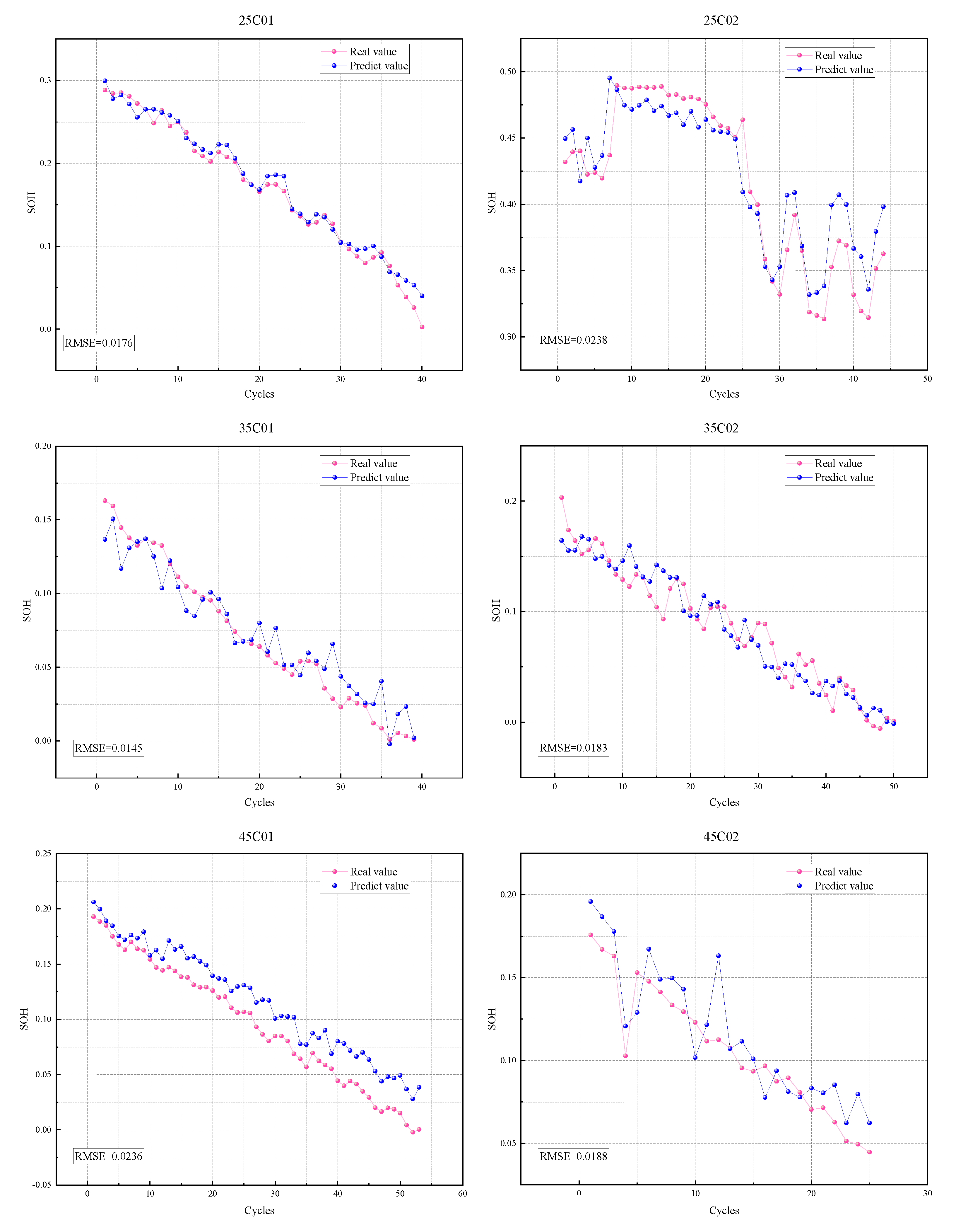
5.6. Prediction and Evaluation of SOH

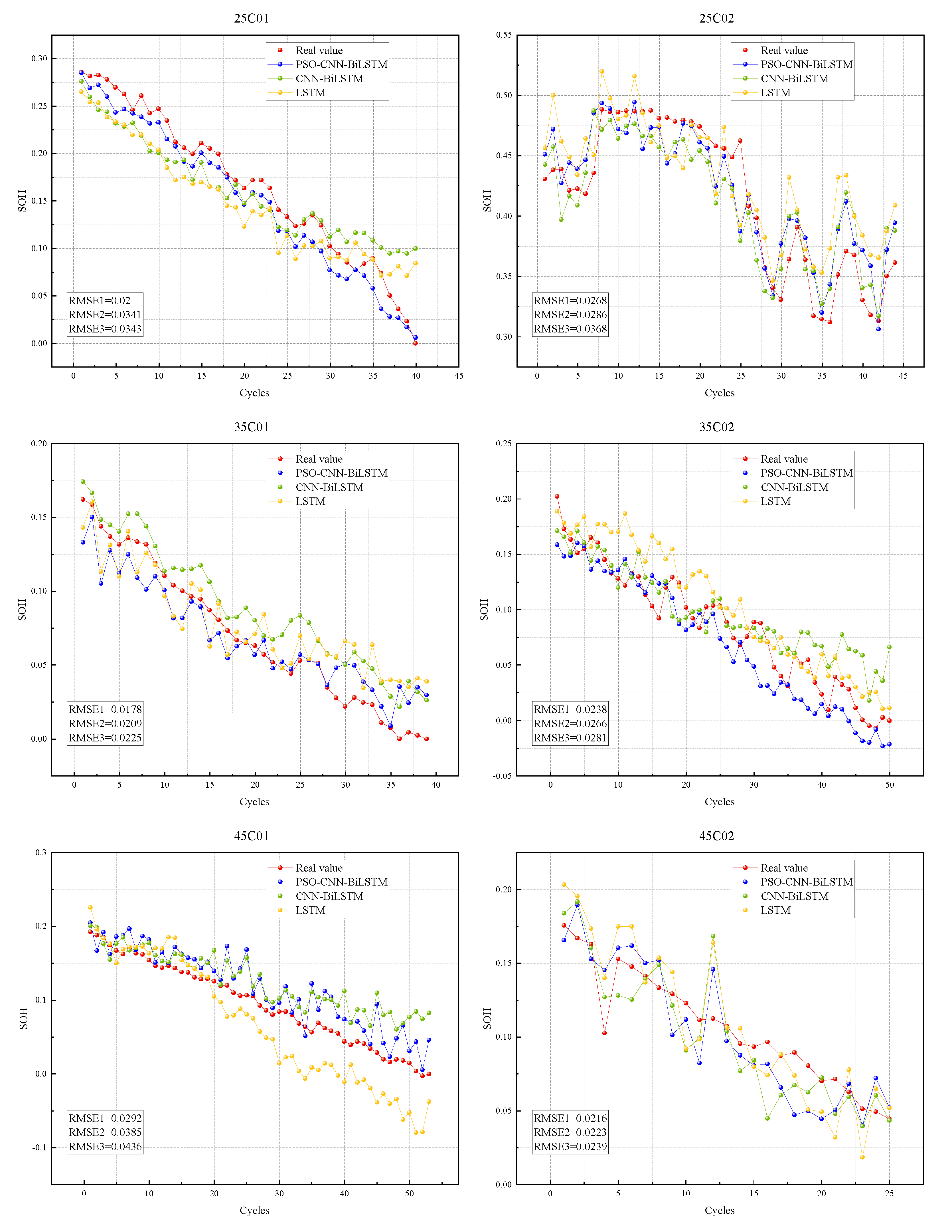
5.6.1. Analysis of Results

It utilizes the predicting models of IPSO-CNN-BiLSTM and estimates the SOH of LIBs at various temperatures. To enter the EIS data into the model, and the training set-to-testing set ratio was 6:4. The results displayed as shown in Figure 8.

From the experimental results, the SOH prediction results are satisfactory. The model results show that the models are not affected by temperature as well as more robustness, can effectively estimate the SOH of LIBs under different working environments. Additionally, the capacity regeneration phenomenon occurs in the process of the aging cycle, because of the indeterminacy of aging mechanism. The proposed model can also response with this phenomenon excellently.

5.6.2. Comparison with Other Models

In order to evaluate the performance of our model, we have compared experimental results with the other three methods (PSO–CNN–BiLSTM, CNN–BiLSTM, LSTM), using the same training and testing data. As shown in Figure 9, the IPSO–CNN–BiLSTM has better accuracy than the traditional PSO–CNN–BiLSTM. With not preprocess the data of LSTM, the noise in the EIS data greatly affects the estimation accuracy; this also indicated the necessity of using the CNN model.

As shown in

Table 7. The RMSE of different models for LIBs.

	25C01	25C02	35C01	35C02	45C01	45C02
IPSO-CNN-BiLSTM	0.0176	0.0238	0.0145	0.0183	0.0236	0.0188
PSO-CNN-BiLSTM	0.02	0.0268	0.0178	0.0238	0.0292	0.0216
CNN-BiLSTM	0.0341	0.0286	0.0209	0.0266	0.0385	0.0223
LSTM	0.0343	0.0368	0.0225	0.0281	0.0436	0.0239

, the comparison results demonstrate that IPSO–CNN–BiLSTM gives better accuracy than other models for LIBs SOH prediction. The improved PSO algorithm performs better than the traditional PSO and may avoid falling into the local optimum instead. Compared to the other three models, the estimation accuracy of IPSO–CNN–BiLSTM increased by 13.6%, 93.75% and 94.8%, respectively (25C01). The simulation results show the presented quick training algorithm can speed up the learning process of IPSO–CNN–BiLSTM and improve the learning properties on convergence and robust performance.

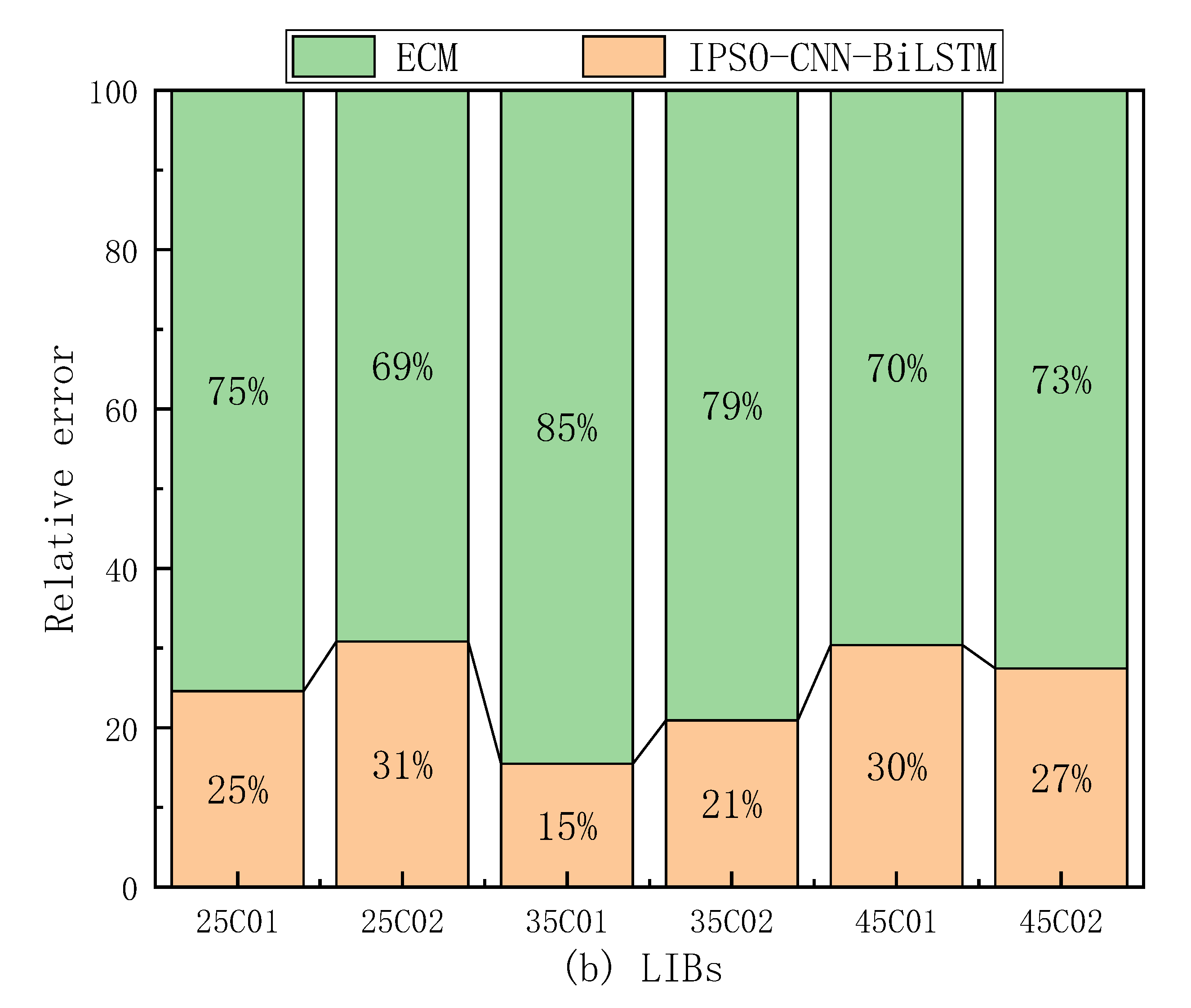
6. Comprehensive Analysis of Data-Driven Method and Model-Based Method

As shown in Figure 10a, improved ECM model and IPSO-CNN-BILSTM model are compared with the basic ECM and data driven method (GPR) [25,36]. The RMSE all showed obvious improvement. As compared with the traditional methods, the RMSE of improved method, which reduce by 17.9% and 63.6% respectively. The performance of the proposed approach is demonstrated by several examples. It is worth noting that the current basic methods only focus on the real and imaginary parts of EIS when extracting impedance features. In the GPR model, the imaginary part of impedance at low frequency is used; these methods ignore the important features of modulus value and phase in EIS data. When selecting the input of the neural network model, we take all the EIS data, which makes the feature extraction more comprehensive and is conducive to reducing the estimation error (RMSE). In addition, enhancing the robustness of the model is also crucial to reduce the estimation error. For the method based on ECM, scientific and accurate EIS data are crucial for model fitting. Once there is an error in the EIS data, double-layer errors will occur in ECM fitting and SOH prediction, which will lead to greater RMSE. In addition, the accurate ECM is also the most effective in reducing the RMSE.

But beyond that, IPSO-CNN-BiLSTM has better prediction accuracy than improved ECM model (Figure 10b). Because the ECM based on the chemical system, which has a very complex mechanism, it brings about relative high requirements on modeling, solving and optimizing models theoretically. During estimating SOH, the effect of this will lead to serious errors; that is to say, the data-driven models, which apparently had more advantages.

7. Conclusions and Outlook

As clean energy, the effect of LIBs in the new generation power is crucial. However, an important problem with LIBs is how to accurately predict their SOH. Aiming at the deficiencies of ECM and data-driven methods currently, this paper puts forward two improvement methods of estimating SOH based on EIS.

(1)

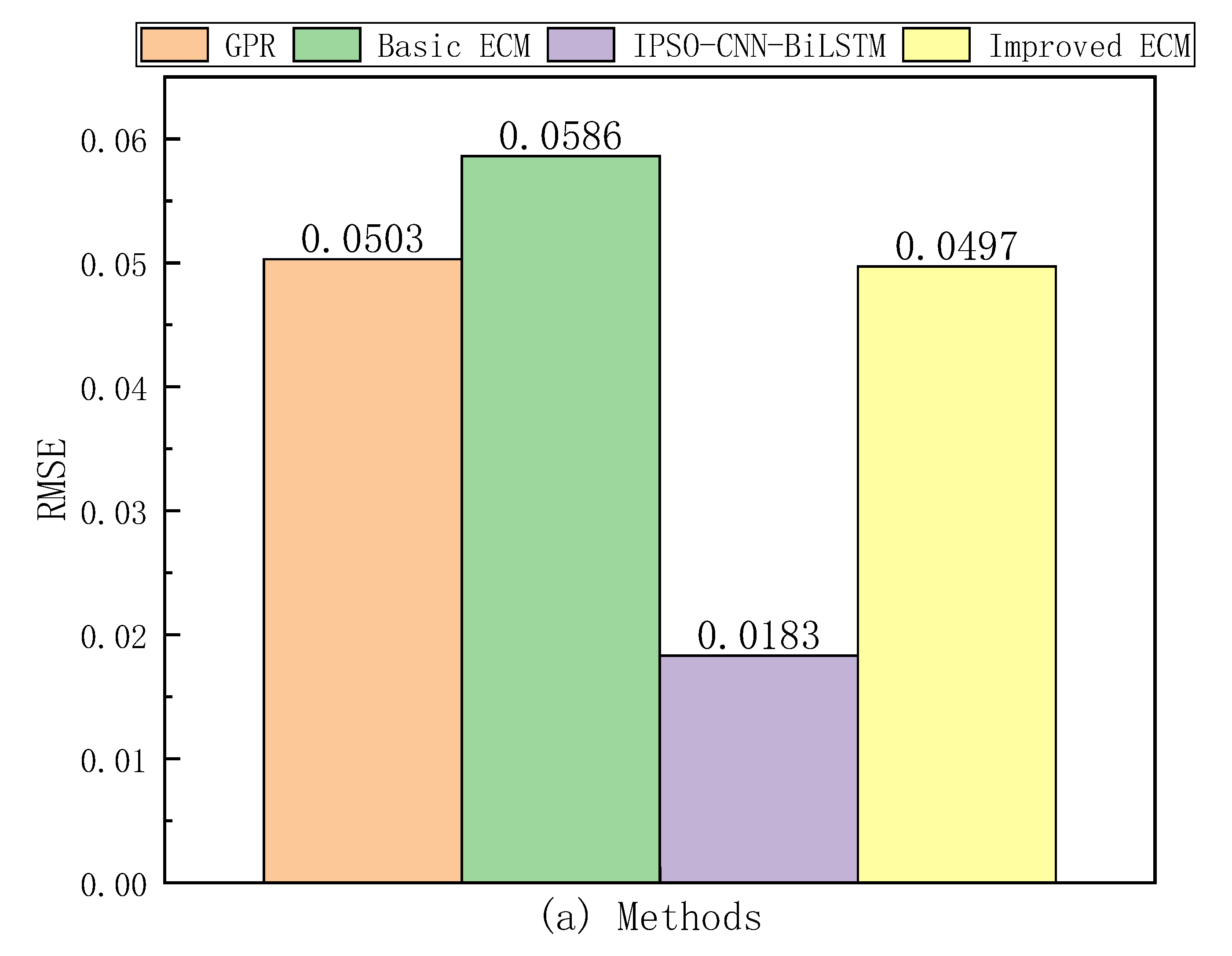
EIS data was used to estimate ECM, which can reduce the estimate error of SOH caused by the imperfect ECM. The method had greatly improved the accuracy for ECM. As compared with the GPR model, the R² coefficient, which increase 34.63%. The performance of the proposed approach is demonstrated.

(2)

CNN is used to process EIS data, it is proved his algorithm can not only extract the key points, but also guarantee the simplified of the feature extraction; moreover, it is prone to realize in fact with broad applicability. BiLSTM model was used for serial regression prediction, the time dependence of EIS data and SOH can be sufficient considered. Then, the CNN-BiLSTM model was optimized based on the IPSO algorithm. The estimation results indicated that compared with the GPR, PSO-CNN-BiLSTM, CNN-BiLSTM and LSTM models, the performance increased 27%, 23.7%, 63% and 84.7% respectively. The practice has proved that the method will improve the precision of SOH forecasting effectively and has excellent robusticity.

However, measuring the EIS of LIBs is still an important challenge. The aging mechanism still unclear, which is the essential cause of SOH estimation disabilities. Although the data-driven model has good performance, the amount of data are insufficient will bring large error. The main difficulties and the opening problems of the estimation of SOH as shown in below.

(1)

Simplified the measuring device of EIS and improved the measuring speed. Binary modules are used to obtain the EIS data will be the main direction for the next research step.

(2)

Numerical simulation of the dendritic growth process, SEI and capacity regeneration are still one of the most interested fields in the aging process of LIBs which is essential for accurate ECM establishment.

(3)

The application of the data-driven algorithm is restricted by the depends on historical data excessively. Under the circumstance of reducing the training data, ensure the model robustness and precision is precisely the challenge ahead.

References

1. Cui, Z.; Dai, J.; Sun, J.; Li, D.; Wang, L.; Wang, K. Hybrid methods using neural network and Kalman filter for the state of charge estimation of lithium-ion battery. Math. Probl. Eng. 2022, 2022, 9616124. [Google Scholar] [CrossRef]
2. Kang, L.; Du, H.; Deng, J.; Jing, X.; Zhang, S.; Znang, Y. Synthesis and Catalytic Performance of a New V-doped CeO2-supported Alkali-activated-steel-slag-based Photocatalyst. J. Wuhan Univ. Technol. Mater. Sci. Ed. 2021, 36, 209–214. [Google Scholar] [CrossRef]
3. Zhou, W.; Du, H.; Kang, L.; Du, X.; Shi, Y.; Qiang, X.; Li, H.; Zhao, J. Microstructure Evolution and Improved Permeability of Ceramic Waste-Based Bricks. Materials 2022, 15, 1130. [Google Scholar] [CrossRef] [PubMed]
4. Saha, B.; Goebel, K.; Poll, S.; Christophersen, J. Prognostics methods for battery health monitoring using a bayesian framework. IEEE Trans. Instrum. Meas. 2009, 58, 291–296. [Google Scholar] [CrossRef]
5. Mc Carthy, K.; Gullapalli, H.; Kennedy, T. Real-time internal temperature estimation of commercial Li-ion batteries using online impedance measurements. J. Power Sources 2022, 519, 230786. [Google Scholar] [CrossRef]
6. Liu, C.; Li, D.; Wang, L.; Li, L.; Wang, K. Strong Robustness and High Accuracy Remaining Useful Life Prediction on Supercapacitors. APL Mater. 2022, 10, 061106. [Google Scholar] [CrossRef]
7. Liu, C.; Zhang, Y.; Sun, J.; Cui, Z.; Wang, K. Stacked bidirectional LSTM RNN to evaluate the remaining useful life of supercapacitor. Int. J. Energy Res. 2022, 46, 3034–3043. [Google Scholar] [CrossRef]
8. Wu, K.; Gu, J.; Meng, L.; Wen, H.; Ma, J. An explainable framework for load forecasting of a regional integrated energy system based on coupled features and multi-task learning. Prot. Control Mod. Power Syst. 2022, 7, 24. [Google Scholar] [CrossRef]
9. Ran, H.; Du, H.; Ma, C.; Zhao, Y.; Feng, D.; Xu, H. Effects of A/B-Site Co-Doping on Microstructure and Dielectric Thermal Stability of AgNbO3 Ceramics. Sci. Adv. Mater. 2021, 13, 741–747. [Google Scholar] [CrossRef]
10. Liu, C.; Li, Q.; Wang, K. State-of-charge estimation and remaining useful life prediction of supercapacitors. Renew. Sustain. Energy Rev. 2021, 150, 111408. [Google Scholar] [CrossRef]
11. Xu, H.; Du, H.; Kang, L.; Cheng, Q.; Feng, D.; Xia, S. Constructing Straight Pores and Improving Mechanical Properties of Gangue-Based Porous Ceramics. J. Renew. Mater. 2021, 9, 2129–2141. [Google Scholar] [CrossRef]
12. Yi, Z.; Zhao, K.; Sun, J.; Wang, L.; Wang, K.; Ma, Y. Prediction of the Remaining Useful Life of Supercapacitors. Math. Probl. Eng. 2022, 2022, 7620382. [Google Scholar] [CrossRef]
13. Ma, C.; Du, H.; Liu, J.; Kang, L.; Du, X.; Xi, X.; Ran, H. High-temperature stability of dielectric and energy-storage properties of weakly-coupled relaxor (1-x)BaTiO3-xBi(Y1/3Ti1/2)O3 ceramics. Ceram. Int. 2021, 47, 25029–25036. [Google Scholar] [CrossRef]
14. Li, X.K.; Su, J.; Li, Z.H.; Zhao, Z.Q.; Zhang, F.L.; Zhang, L.Q.; Ye, W.N.; Li, Q.H.; Wang, K.; Wang, X.; et al. Revealing interfacial space charge storage of Li+/Na+/K+ by operando magnetometry. Sci. Bull. 2022, 67, 1145–1153. [Google Scholar] [CrossRef]
15. Chang, C.; Wang, S.; Jiang, J.; Gao, Y.; Jiang, Y.; Liao, L. Lithium-ion battery state of health estimation based on electrochemical impedance spectroscopy and cuckoo search algorithm optimized elman neural network. J. Electrochem. Energy Convers. Storage 2022, 19, 1–11. [Google Scholar] [CrossRef]
16. Nara, H.; Yokoshima, T.; Osaka, T. Technology of electrochemical impedance spectroscopy for an energy-sustainable society. Curr. Opin. Electrochem. 2020, 20, 66–77. [Google Scholar] [CrossRef]
17. Gaberscek, M. Understanding Li-based battery materials via electrochemical impedance spectroscopy. Nat. Commun. 2021, 12, 6513. [Google Scholar] [CrossRef]
18. Li, Q.; Li, D.; Zhao, K.; Wang, L.; Wang, K. State of health estimation of lithium-ion battery based on improved ant lion optimization and support vector regression. J. Energy Storage 2022, 50, 104215. [Google Scholar] [CrossRef]
19. Padhy, S.; Panda, S. Application of a simplified Grey Wolf optimization technique for adaptive fuzzy PID controller design for frequency regulation of a distributed power generation system. Prot. Control Mod. Power Syst. 2021, 6, 2. [Google Scholar] [CrossRef]
20. Cui, Z.; Kang, L.; Li, L.; Wang, L.; Wang, K. A combined state-of-charge estimation method for lithium-ion battery using an improved BGRU network and UKF. Energy 2022, 259, 124933. [Google Scholar] [CrossRef]
21. Cui, Z.; Wang, L.; Li, Q.; Wang, K. A comprehensive review on the state of charge estimation for lithium-ion battery based on neural network. Int. J. Energy Res. 2022, 46, 5423–5440. [Google Scholar] [CrossRef]
22. Pulido, Y.F.; Blanco, C.; Ansean, D.; Garcia, V.M.; Ferrero, F.; Valledor, M. Determination of suitable parameters for battery analysis by Electrochemical Impedance Spectroscopy. Measurement 2017, 106, 1–11. [Google Scholar] [CrossRef]
23. Galeotti, M.; Cina, L.; Giammanco, C.; Cordiner, S.; Di Carlo, A. Performance analysis and SOH (state of health) evaluation of lithium polymer batteries through electrochemical impedance spectroscopy. Energy 2015, 89, 678–686. [Google Scholar] [CrossRef]
24. Wang, X.Y.; Wei, X.Z.; Dai, H.F. Estimation of state of health of lithium-ion batteries based on charge transfer resistance considering different temperature and state of charge. J. Energy Storage 2019, 21, 618–631. [Google Scholar] [CrossRef]
25. Zhang, Q.; Huang, C.-G.; Li, H.; Feng, G.; Peng, W. Electrochemical impedance spectroscopy based state of health estimation for Lithium-ion battery considering temperature and state of charge effect. IEEE Trans. Transp. Electrif. 2022. [Google Scholar] [CrossRef]
26. Li, D.; Wang, L.; Duan, C.; Li, Q.; Wang, K. Temperature prediction of lithium-ion batteries based on electrochemical impedance spectrum: A review. Int. J. Energy Res. 2022, 46, 10372–10388. [Google Scholar] [CrossRef]
27. Kalyan, C.H.; Rao, G.S. Impact of communication time delays on combined LFC and AVR of a multi-area hybrid system with IPFC-RFBs coordinated control strategy. Prot. Control Mod. Power Syst. 2021, 6, 7. [Google Scholar] [CrossRef]
28. Saikrishna, R.; Rajalwal, N.K.; Ghosh, D. Adaptive relay co-ordination using a busbar splitting approach for a system integrity protection scheme. Prot. Control Mod. Power Syst. 2022, 7, 14. [Google Scholar] [CrossRef]
29. Sakthivel, V.P.; Sathya, P.D. Single and multi-area multi-fuel economic dispatch using a fuzzified squirrel search algorithm. Prot. Control Mod. Power Syst. 2021, 6, 11. [Google Scholar] [CrossRef]
30. Sun, H.; Sun, J.; Zhao, K.; Wang, L.; Wang, K. Data-driven ICA-Bi-LSTM-combined lithium battery SOH estimation. Math. Probl. Eng. 2022, 2022, 9645892. [Google Scholar] [CrossRef]
31. Li, D.; Li, S.; Zhang, S.; Sun, J.; Wang, L.; Wang, K. Aging state prediction for supercapacitors based on heuristic kalman filter optimization extreme learning machine. Energy 2022, 250, 123773. [Google Scholar] [CrossRef]
32. Hu, C.; Cai, Z.; Zhang, Y.; Yan, R.; Cai, Y.; Cen, B. A soft actor-critic deep reinforcement learning method for multi-timescale coordinated operation of microgrids. Prot. Control Mod. Power Syst. 2022, 7, 29. [Google Scholar] [CrossRef]
33. Hua, Y.; Wang, N.; Zhao, K. Simultaneous Unknown Input and State Estimation for the Linear System with a Rank-Deficient Distribution Matrix. Math. Probl. Eng. 2021, 2021, 6693690. [Google Scholar] [CrossRef]
34. Sun, H.L.; Yang, D.F.; Wang, L.C.; Wang, K. A method for estimating the aging state of lithium-ion batteries based on a multi-linear integrated model. Int. J. Energy Res. 2022. [Google Scholar] [CrossRef]
35. Cui, Z.; Kang, L.; Li, L.; Wang, L.; Wang, K. A hybrid neural network model with improved input for state of charge estimation of lithium-ion battery at low temperatures. Renew. Energy 2022, 198, 1328–1340. [Google Scholar] [CrossRef]
36. Zhang, Y.W.; Tang, Q.C.; Zhang, Y.; Wang, J.B.; Stimming, U.; Lee, A.A. Identifying degradation patterns of lithium ion batteries from impedance spectroscopy using machine learning. Nat. Commun. 2020, 11, 1706. [Google Scholar] [CrossRef]
37. Guo, Y.; Yu, P.; Zhu, C.; Zhao, K.; Wang, L.C.; Wang, K. A state-of-health estimation method considering capacity recovery of lithium batteries. Int. J. Energy Res. 2022. [Google Scholar] [CrossRef]
38. Messing, M.; Shoa, T.; Ahmed, R.; Habibi, S. Battery SOC estimation from EIS using neural nets. In Proceedings of the IEEE Transportation Electrification Conference and Expo (ITEC), Chicago, IL, USA, 23–26 June 2020; pp. 588–593. [Google Scholar]
39. Li, Y.G.; Dong, B.; Zerrin, T.; Jauregui, E.; Wang, X.C.; Hua, X.; Ravichandran, D.; Shang, R.X.; Xie, J.; Ozkan, M.; et al. State-of-health prediction for lithium-ion batteries via electrochemical impedance spectroscopy and artificial neural networks. Energy Storage 2020, 2, e186. [Google Scholar] [CrossRef]
40. Lyu, C.; Zhang, T.; Luo, W.L.; Wei, G.; Ma, B.Z.; Wang, L.X. SOH estimation of Lithium-ion batteries based on fast time domain impedance spectroscopy. In Proceedings of the 14th IEEE Conference on Industrial Electronics and Applications (ICIEA), Xi’an, China, 19–21 June 2019; pp. 2142–2147. [Google Scholar]
41. Che, Y.H.; Deng, Z.W.; Li, P.H.; Tang, X.L.; Khosravinia, K.; Lin, X.K.; Hu, X.S. State of health prognostics for series battery packs: A universal deep learning method. Energy 2022, 238, 121857. [Google Scholar] [CrossRef]
42. Rui, X.; Jinpeng, T.; Hao, M.; Chun, W. A system aticmodel-based degradation behavior recognition and health monitoring method for lithium-ion batteries. Appl. Energy 2017, 207, 372–383. [Google Scholar]
43. Eddahech, A.; Briat, O.; Bertrand, N.; Deletage, J.Y.; Vinassa, J.M. Behavior and state-of-health monitoring of Li-ion batteries using impedence spectroscopy and recurrent neural networks. Int. J. Electr. Power Energy Syst. 2012, 42, 487–494. [Google Scholar] [CrossRef]
44. Pradyumna, T.K.; Cho, K.; Kim, M.; Choi, W. Capacity estimation of lithium-ion batteries using convolutional neural network and impedance spectra. J. Power Electron. 2022, 22, 850–858. [Google Scholar] [CrossRef]
45. Ivers-Tiffee, E.; Weber, A. Evaluation of electrochemical impedance spectra by the distribution of relaxation times. J. Ceram. Soc. Jpn. 2017, 125, 193–201. [Google Scholar] [CrossRef]
46. Schonleber, M.; Klotz, D.; Ivers-Tiffee, E. A method for improving the robustness of linear kramers-kronig validity tests. Electrochim. Acta 2014, 131, 20–27. [Google Scholar] [CrossRef]
47. Talian, S.D.; Moskon, J.; Dominko, R.; Gaberscek, M. The pitfalls and opportunities of impedance spectroscopy of lithium sulfur batteries. Adv. Mater. Interfaces 2022, 9, 2101116. [Google Scholar] [CrossRef]
48. Feng, D.; Du, H.; Ran, H.; Lu, T.; Xia, S.; Xu, L.; Wang, Z.; Ma, C. Antiferroelectric stability and energy storage properties of Co-doped AgNbO3 ceramics. J. Solid State Chem. 2022, 310, 123081. [Google Scholar] [CrossRef]
49. Birkl, C.R.; Roberts, M.R.; McTurk, E.; Bruce, P.G.; Howey, D.A. Degradation diagnostics for lithium ion cells. J. Power Sources 2017, 341, 373–386. [Google Scholar] [CrossRef]
50. Pop, V.; Bergveld, H.J.; Regtien, P.P.; het Veld, J.O.; Danilov, D.; Notten, P.H.L. Battery aging and its influence on the electromotive force. J. Electrochem. Soc. 2007, 154, A744–A750. [Google Scholar] [CrossRef]
51. Kassem, M.; Delacourt, C. Postmortem analysis of calendar-aged graphite/LiFePO4 cells. J. Power Sources 2013, 235, 159–171. [Google Scholar] [CrossRef]
52. Dubarry, M.; Truchot, C.; Liaw, B.Y. Synthesize battery degradation modes via a diagnostic and prognostic model. J. Power Sources 2012, 219, 204–216. [Google Scholar] [CrossRef]
53. Agubra, V.; Fergus, J. Lithium-ion battery anode aging mechanisms. Materials 2013, 6, 1310–1325. [Google Scholar] [CrossRef] [PubMed] [Green Version]
54. Ren, L.; Dong, J.B.; Wang, X.K.; Meng, Z.H.; Zhao, L.; Deen, M.J. A Data-Driven Auto-CNN-LSTM prediction model for lithium-ion battery remaining useful life. IEEE Trans. Ind. Inform. 2021, 17, 3478–3487. [Google Scholar] [CrossRef]
55. Fu, Y.P.; Hou, Y.S.; Wang, Z.F.; Wu, X.W.; Gao, K.Z.; Wang, L. Distributed scheduling problems in intelligent manufacturing systems. Tsinghua Sci. Technol. 2021, 26, 625–645. [Google Scholar] [CrossRef]
56. Jiang, J.; Zhang, T.; Chen, D. Analysis, Design, and Implementation of a Differential Power Processing DMPPT With Multiple Buck–Boost Choppers for Photovoltaic Module. IEEE Trans. Power Electron. 2021, 36, 10214–10223. [Google Scholar] [CrossRef]
57. Fu, Y.P.; Wang, H.F.; Tian, G.D.; Li, Z.W.; Hu, H.S. Two-agent stochastic flow shop deteriorating scheduling via a hybrid multi-objective evolutionary algorithm. J. Intell. Manuf. 2019, 30, 2257–2272. [Google Scholar] [CrossRef]
Figure 1. (a) Aging and EIS impedance test diagram. (b) The capacity attenuation curves of LIBs at different temperatures. (c) Impedance curve as the number of battery cycles increases.
Energies 15 06665 g001
Figure 2. The ECM of measured EIS data.
Energies 15 06665 g002
Figure 3. Lin—KK test flow chart.
Energies 15 06665 g003
Figure 4. (a,b) Residual of EIS at different SOC, 25 °C under Lin–KK test. (c,d) Residual of EIS at different SOC, 35 °C under Lin–KK test. (e,f) Residual of EIS at different SOC, 45 °C under Lin–KK test.
Energies 15 06665 g004
Figure 5. ECM of LIBs (a) EIS curves and their corresponding ECM elements. (b) The different ECM models of LIBs.
Energies 15 06665 g005
Figure 6. Curves of different parameters as the number of cycles increases.
Energies 15 06665 g006
Figure 7. The diagram of IPSO-CNN-BiLSTM model.
Energies 15 06665 g007
Figure 8. Prediction results of IPSO–CNN–BiLSTM for LIBs.
Energies 15 06665 g008
Figure 9. Comparison prediction results of different models for LIBs.
Energies 15 06665 g009
Figure 10. (a) Comparison of RMSE coefficient between the proposed improved model and the traditional models. (b) Comparison of relative errors between ECM model and IPSO-CNN-BILSTM model.
Energies 15 06665 g010aEnergies 15 06665 g010b