Article

Performance and Efficiency Trade-Offs in Brazilian Passenger Vehicle Fleet

by
Rafael Fernandes Mosquim
1,† and
Carlos Eduardo Keutenedjian Mady
2,*,†
1
School of Mechanical Engineering, University of Campinas, Campinas 13083-970, Brazil
2
Department of Mechanical Engineering, Centro Universitário FEI, São Bernardo do Campo 09850-901, Brazil
*
Author to whom correspondence should be addressed.
These authors contributed equally to this work.
Energies 2022, 15(15), 5416; https://doi.org/10.3390/en15155416
Submission received: 5 July 2022 / Revised: 22 July 2022 / Accepted: 23 July 2022 / Published: 27 July 2022
(This article belongs to the Topic Energy Saving and Energy Efficiency Technologies)

Abstract

:
The rate of technological progress is an important metric used for predicting the energy consumption and greenhouse gas emissions of future light-duty fleets. A trade-off between efficiency and performance is essential due to its implications on fuel consumption and efficiency improvement. These values are not directly available in the Brazilian fleet. Hence, this is the main gap in knowledge that has to be overcome. Tendencies in all relevant parameters were also unknown, and we have traced them as well, established on several publications data and models. We estimate the three indicators mentioned above for the Brazilian fleet from 1990 to 2020. Although the rate of technological progress was lower in Brazil than that in developed countries, it has increased from 0.39% to 0.61% to 1.7% to 1.9% in subsequent decades. Performance improvements offset approximately 31% to 39% of these efficiency gains. Moreover, the vehicle market is shifting toward larger vehicles, thus offsetting some efficiency improvements. We predict the fleet fuel efficiency for the years 2030 and 2035 using the above-mentioned factors. The predicted values for efficiency can vary by a factor of two. Thus, trade-off policies play a vital role in steering toward the desired goals of reducing the transportation sector’s impact on the environment.

Graphical Abstract

1. Introduction

The transportation sector is one of the primary energy consumers globally. The sector’s share of total energy consumption represented 25% in 1990 and 33% in 2020 in Brazil. Fuel use increased by 83.3% between 2004 and 2018. Light-duty vehicles (LDVs), used for personal transportation, account for about half of the total energy consumed by the transportation sector; the remaining energy is consumed by heavy trucks and used for cargo transportation [1].
Due to technological advancements, LDVs have become faster, more powerful, larger, and heavier today. Furthermore, it is safer, causes less impact on the environment, and uses fuel more efficiently.
The first fundamental aspect considered in this study is to estimate the rate of technological improvement for the LDV fleet in Brazil for the period 1990–2020. The two main approaches to assess this are as follows: (1) to estimate the extra amount of fuel that would have been consumed if not for these advancements [2] or (2) to assess technological evolution in a broader sense, meaning either better efficiency or more performance [3,4]. The key insight is that efficiency has to be traded-off for performance; thus, theoretical technological gains are not always translated into more efficiency. If these trade-offs are not adequately considered, projections can be overly optimistic.
It should be noted that in this study, FE represents the number of kilometers that can be traveled by consuming one liter of fuel (km/L). This unity system is analogous to the miles per gallon (MPG) unit system used in the United States (10 km/L is equal to 23.52 MPG). In Europe, fuel efficiency is considered as the relationship between fuel consumed and distance traveled (i.e., liters per 100 km). The relationship between both metrics is not linear but curvilinear, and this may cause misconceptions regarding fuel savings [5]. In this study, improved FE and efficiency are used interchangeably, and both terms indicate an increase in km/L.
The second aspect considered in this study is the dynamic nature of the LDV market. Consumer preferences may shift toward heavier and more powerful vehicle categories, thereby offsetting some or all of the efficiency improvements that might have occurred in individual models. Recently, compact SUVs have gained market share at the expense of the traditional Brazilian vehicle categories: the subcompact and compact models. Such transformation is equivalent, to a lesser extent, to the light-truck reaching half of total sales in the USA from a few percent in the 1970s.
These factors have not been thoroughly studied for the transportation sector of Brazil, and future scenarios are usually predicted using the data from a limited set of years (there are insufficient government data in Brazil for these predictions as in the USA. From a study conducted by Mosquim and Mady [6], the following key insights into the technological developments between 1970 and 2020 were obtained. First, the rate of technological progress during this period and the changes in these rates between decades were observed. Second, the consequences of significant consumer preference shift were identified. These findings could help policymakers improve projections.
The final aspect considered in this study is the hybridization of LDVs. Electricity is a prospective fuel for LDVs. Hybrid-electric and electric vehicles are developed with various degrees of hybridization and by full electrification, respectively. As the market share of hybrid LDVs in Brazil is still low, accounting for 2% of total sales in 2021, internal combustion engines (ICEs) are expected to power a vast majority of vehicles in the near future [7]. In Brazil, the discussion about the transition of the vehicle fleet toward electrification is not straightforward [8] as there are numerous factors involved in the development of this technology. First, researchers agree that owing to the Brazilian reality of biofuels, the transition across regions may differ; thus, it must respect the regionalities and accommodate accordingly to avoid a higher carbon transportation system [9]. Second, the fuel production from second-generation biomass, i.e., from a different source of biomass [10]. Third, CO2 emissions during vehicle transportation for battery recycling [11,12]. There exist certain questions including whether any guarantee can be provided such that the biorefinery production occurs with minimum or negative carbon production [13]. Each country has its own characteristics, a case-by-case study may be conducted in order to achieve a more sustainable transportation sector and with correct transitions [12,14].
Thus, the objectives are to study the FE of Brazil’s LDV fleet and the factors that affect it. First, we applied regression analysis to estimate the rate of technological improvements during the 1990 to 2020 period. Next, we assessed the impact of certain vehicle features, such as weight and power, and certain engine and power-train technologies on FE. Furthermore, we evaluated the trade-offs between performance and efficiency and market evolution. Finally, we simulated a few scenarios for predicting the average fleet FE in 2030 and 2035 using the study’s findings.
The remainder of this study is structured as follows. A literature review is provided in Section 2 to discuss previous works and to identify the research gap and course of action. The methods are detailed in Section 3. A brief discussion on the Brazilian LDV market and the evolution of key LDV parameters is provided in Section 4. The regression analysis results and discussion are provided in Section 5.The possible future pathways for key variables that affect fleet FE are discussed in Section 6, and the possible future fleet-wide FE is presented in Section 7. Finally, the main conclusions, policy implications, and opportunities for future research are presented in Section 8.

2. Literature Review

A question researchers frequently ask in the field of transportation is “by how much can technology reduce fuel consumption compared to a baseline scenario?”. Green et al. [2] estimated two trillion gallons of gasoline for the USA from 1975 to 2018, which is approximately the total US LDV energy consumption from 2004 to 2018, or the total GHG emissions for the USA from 2016 to 2018. However, one caveat that the authors acknowledge as not realistic, taken only for illustrative purposes, is that the FE would remain at the 1975 levels. This kind of study can be categorised as “things could have been worse”, and credit technological progress for not allowing that to happen.
An opposite approach acknowledges this technological progress but tries to estimate by how much could efficiency be improved if performances were held to some baseline level. Knittel [3] found that MPG could have been improved by 60% in the period 1980–2006 in the US, if performances were held at 1980 levels. Actual improvements were in the order of 15%; thus, the majority of technological gains was spent in better performance and not efficiency. The quantification of this trade-off is useful in illustrating the choices made regarding where this technological budget was spent. This line of reasoning could be described as “things could have been better”.
Chea et al. [15] identified three main technological options to achieve factor-of-two reductions in fuel consumption in the USA by 2035 (from 2007). They are as follows: (i) to focus future technological developments in reducing fuel consumption, maintaining fixed performance; (ii) market penetration of alternative power trains, such as diesel, turbocharged gasoline, and hybrids; and (iii) weight and size reductions. Their findings suggest that only a combination of these three pathways can achieve the stated goal and that it would take “striking changes from the status quo”. For example, estimated values for 2020 would be approximately 32 MPG, whereas the actual values were 25.4 MPG, which is still record-high [16].
We revised a few works on the LDV fleet in Brazil, identified certain critical assumptions made, and compared them with actual developments. Certain simplifications are inevitable, particularly when trying to quantify the total GHG emissions, which are dependent on several variables (including the number of cars with better efficiency) and presented in Section 7.1. By decomposing the more significant problem and delving deeper into a few key variables, this study can improve future models. Here, the assumptions about the rates of efficiency improvements and market share by vehicle classes are given particular interest, both of which impact the fleet FE and, thus, affects the fuel consumption.
Schmitt et al. [17] used numerical simulation to estimate the fuel efficiency of future vehicles. Their approach was to represent the fleet by some vehicle categories, 26 in total, and evaluate the total fuel consumption in two scenarios by comparing it to the baseline. By using some modifications in the technological factor to improve the FE, the following values can be achieved: approximately 9% to 17% of total fuel consumption reductions, which represent a decline in GHG emissions by 9% to 20% and 0.9 to 1.8 million hectares of land spared for other uses. Assumptions for achieving these numbers were as follows: subcompact and compact vehicles would represent approximately 60% of the fleet in 2030 compared to 45% in 2007. Incremental efficiency gains would be 15%. Drag and rolling coefficients would be reduced by 15% and 20%. Moreover, there would be a weight reduction by 10% or 20% in each category. Estimated travel per vehicle would remain constant. As was reported in [
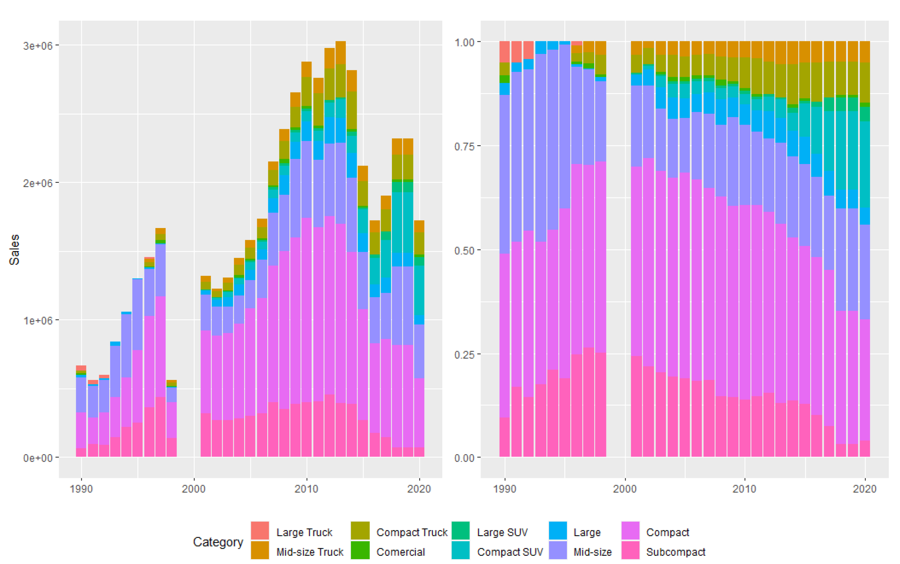
6], although the drag coefficient reduces slightly over time, the frontal area continues increasing as vehicles become larger. Moreover, the sales of subcompact and compact declined steadily from 75% in 2000 to 35% in 2020. In addition, a 1.0 L model year (MY) in 2020 is significantly different from one in 2000 because of improvements in technology and engine downsizing, as engineers can extract more performance today for the same level of power than in the past [4].
Other researchers, including Benvenutti et al. [18,19], estimated future GHG emissions by considering four main strategies for mitigating carbon footprint: improving energy efficiency, a modal shift towards public transport, a renovation of the fleet (older vehicles have higher emission factors), and the increased use of biofuels. Each main strategy had more than one assumption related to its degree of application. Thus, the efficiency scenario was divided into three pathways with variable improvement rates. The more conservative among them was a 2.2% and 2.0% improvement in efficiency per year until 2030 and 2050, respectively. The second had a 3.14% and 2.2%, whereas the third had a 3.8% and 2.0% improvement in efficiency, respectively. According to that study, even the most conservative rate of improvement was higher than the historical rate of 1.6%.
From the point of view of policymakers, De Melo et al. [20] argued about the necessity of mandatory fuel economy standards (MFES), in line with the practices established in the United States, European Union, Japan, China, South Korea, Canada, and Mexico. An extensive discussion about those standards is available in [21]; for an abridged version in English, refer to [22], which focuses on the Brazilian history.
Their method [20] was to estimate the improvements in efficiency exceeding baseline by the implementation of MFES. The average fuel efficiencies for compact and subcompact vehicles were approximately 1.85 MJ/km and 1.66 MJ/km, respectively, in 2017 (MJ/km is obtained by dividing the heating value of fuel in MJ/L by the fuel economy in km/L). The combined market share for these two classes was 65% and remained constant until 2035, the final year of the projections. The MFES was modeled as step-wise improvements by increasing the efficiency by 0.05 MJ/km and 0.08 MJ/km every four years. The results showed potential and avoided emissions of 62 Gg of CO2 compared to the baseline. In reality, the average values for subcompact (19 models) and compact (78 models) in 2020, according to [23], were 1.49 MJ/km and 1.67 MJ/km, which are close to the projected values. Nevertheless, the importance of the article is its reduction perspective. Unfortunately, the market shares of both classes reduced and reached 35% in 2020.
Wills and La Rovere [24] simulated three scenarios from 2000 to 2030, with yearly efficiency improvements of 0.25% (baseline), 1.12% (adjusted), and 2.38% (optimistic). Each scenario denoted 14.2% to 30.7% of energy consumption decrease in 2030. Emissions in 2019 were estimated to be in the range of (35–40) Mton CO2, which was approximately 50% below what was actually observed in Brazil in 2019 [25]. Moreover, the avoided CO2 emissions in 2030 for each scenario were predicted to be 1.3 to 2.6 compared to what was emitted in 2019.
Modeling future energy consumption and GHG emissions can be very tricky. De Andrade Junior et al. [26] employed a highly detailed partial equilibrium model to estimate ethanol demand for the year 2030, along with a sugarcane planted area required to meet such a demand for fuel. Variables used were gross domestic product (GDP), population growth, fuel blend directives, fuel prices, fleet composition, and efficiency gains. Ethanol demand could be 13% to 114% higher in 2030 than in 2018. Moreover, there are numerous known and unknown variables, which affect FE. One of the highest uncertainties is related to future fuel efficiency assumptions. With 2013 data as a baseline, a BAU scenario implies yearly improvements of 1.0%, a renewable fuel-oriented 1.53%, and a fossil fuel-oriented 0%.
De Salvo Jr. et al. [27,28] conducted extensive analyses of engine technology impacts on energy efficiency first for a single year, 2017, and subsequently, compared the evolution over the years 2013, 2015, and 2017. Based on the official labeling program [23], which has published FE for selected LDVs since 2009, they found that the overall efficiency improved by 3.5% from 2013 to 2017. The same observation can be obtained by dividing vehicle categories. Both papers further offer a review of engine technologies, quantify their impacts on efficiency, and trace their diffusion. The analysis focused on the models available in the market in that year; thus, those studies were not concerned with possible sales-weighted effects, such as consumers shifting preference toward a larger class of vehicles over time. However, even if efficiency improves on a class-by-class basis, this sales shift can impact overall efficiency, and Brazilians are showing a tendency to buy larger vehicles, which is discussed in Section 4.4.

Estimating Technological Progress and Trade-Offs

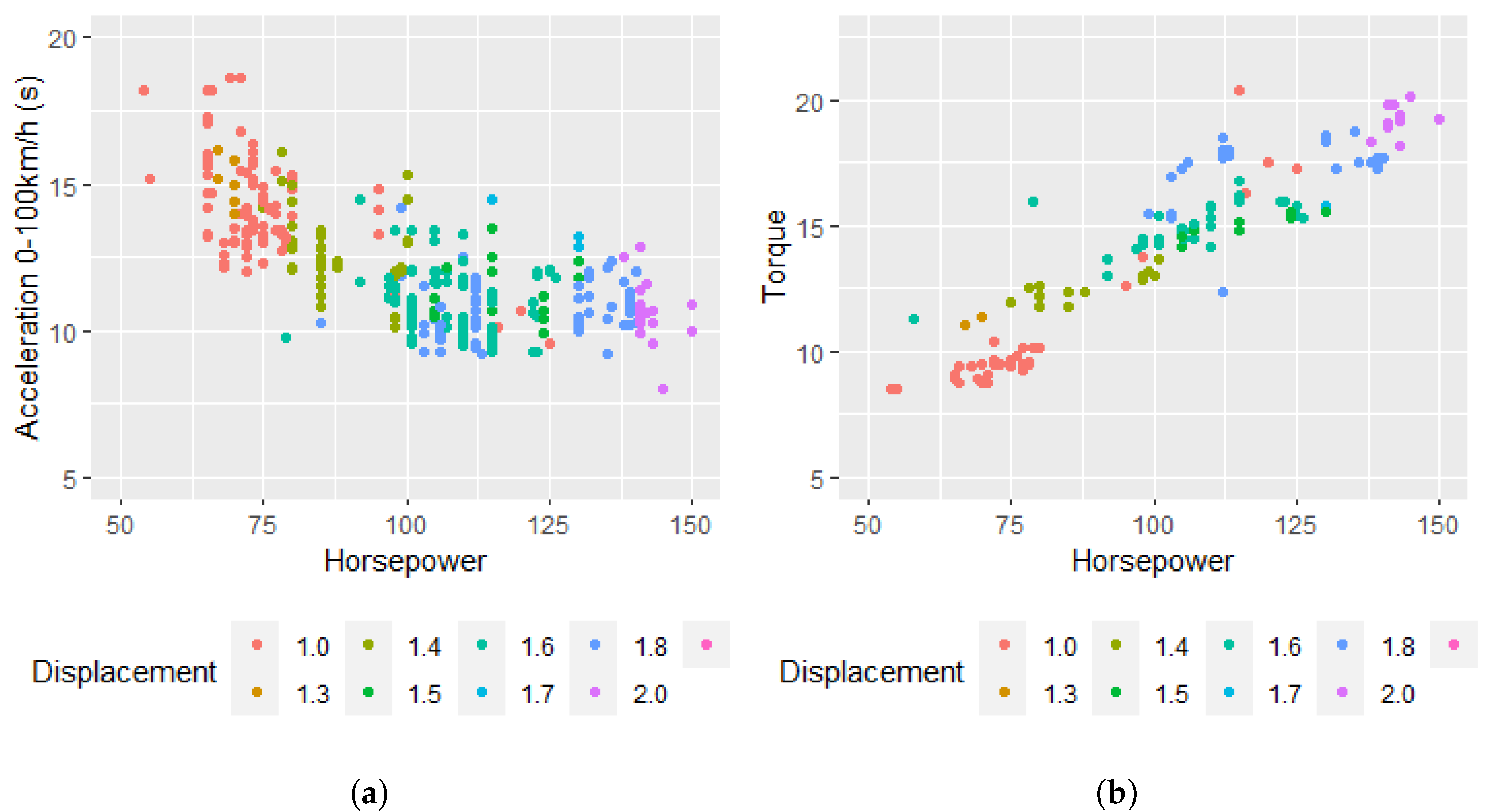
The United States’ Environmental Protection Agency (EPA) publishes vehicle data, as well as sales-weighted averages, going back to 1975. An efficiency metric, ton.mpg, is published as well. Because this metric fails to account for performance improvements and mass efficiency due to lightweight materials, studies based on this data-set tried to establish these efficiency and performance trade-offs [29,30]. The main vehicle features that offset efficiency gains from the use of energy-saving technologies are more performance, which can be modelled as either more torque, horsepower or faster acceleration, which tend to be highly correlated, and more weight, due to increases in size, on-board features, and/or more safety. Mackenzie estimates that features added 223 kg to a vehicle in 2010. Among these, 28% are related to safety, 11% for emission control, and 61% for comfort and convenience [4]. Lutsey and Sperling [29] considered that ton.mpg was insufficient as it does not account for improvements in drag and rolling coefficients or the deployment of drivetrain efficiency technologies. They defined engine and drivetrain efficiency relative to vehicle characteristics, such as mass, acceleration, drag coefficient, frontal area, and tire rolling resistance. Combined with FE data, they estimated the elasticities for the variables mentioned via regression analysis. Thus, it was subsequently possible to estimate trade-offs between efficiency, performance, and size. The FE for cars and light trucks could be 12% higher in 2004 compared with that in 1987 if all technological improvements were directed toward more efficiency. Actual values were 2% higher for LDVs and 3% lower for light trucks.
An and DeCicco [30] identified the same problem with ton.mpg as Lutsey and Sperling did, while using different vehicle attributes for analysis. Consequently, they developed a performance index that could capture trade-offs between size, performance, and FE. Equation (1) presents the performance-size FE index ( P S F I ) for light-duty vehicles. The term H P is the horse-power, L B is the weight in (lb), M P G is the engine consumption in miles per gallons, and F T 3 is the interior volume in cubic feet.
P S F I = P . S . F = H P L B × F T 3 × M P G
Their results [30] indicate that P S F I increased linearly from 1977 to 2005. Another inference was that no FE gains were realized in the period by keeping size and performance fixed, and a warn was made for prospective studies to consider this important fact. 
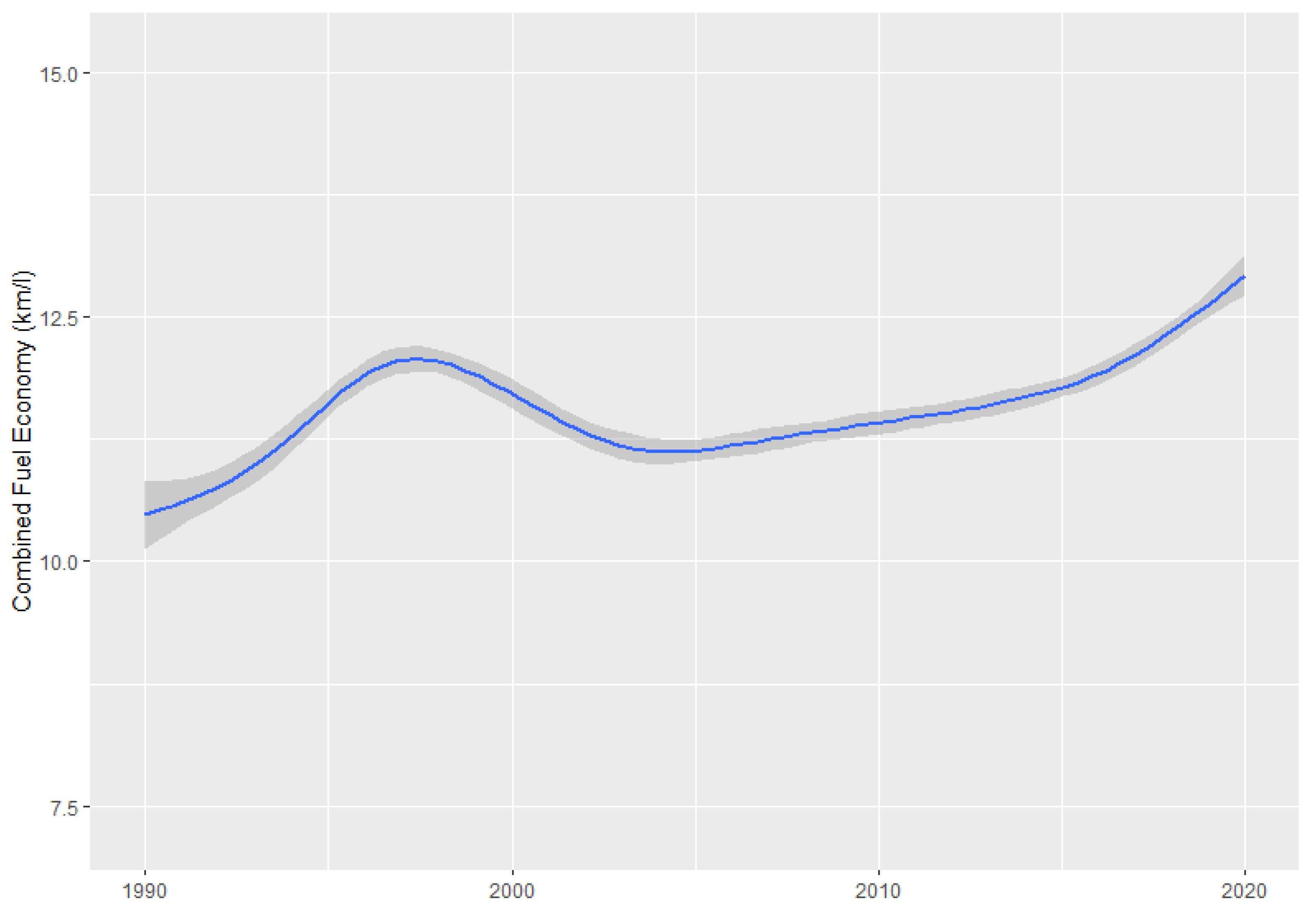
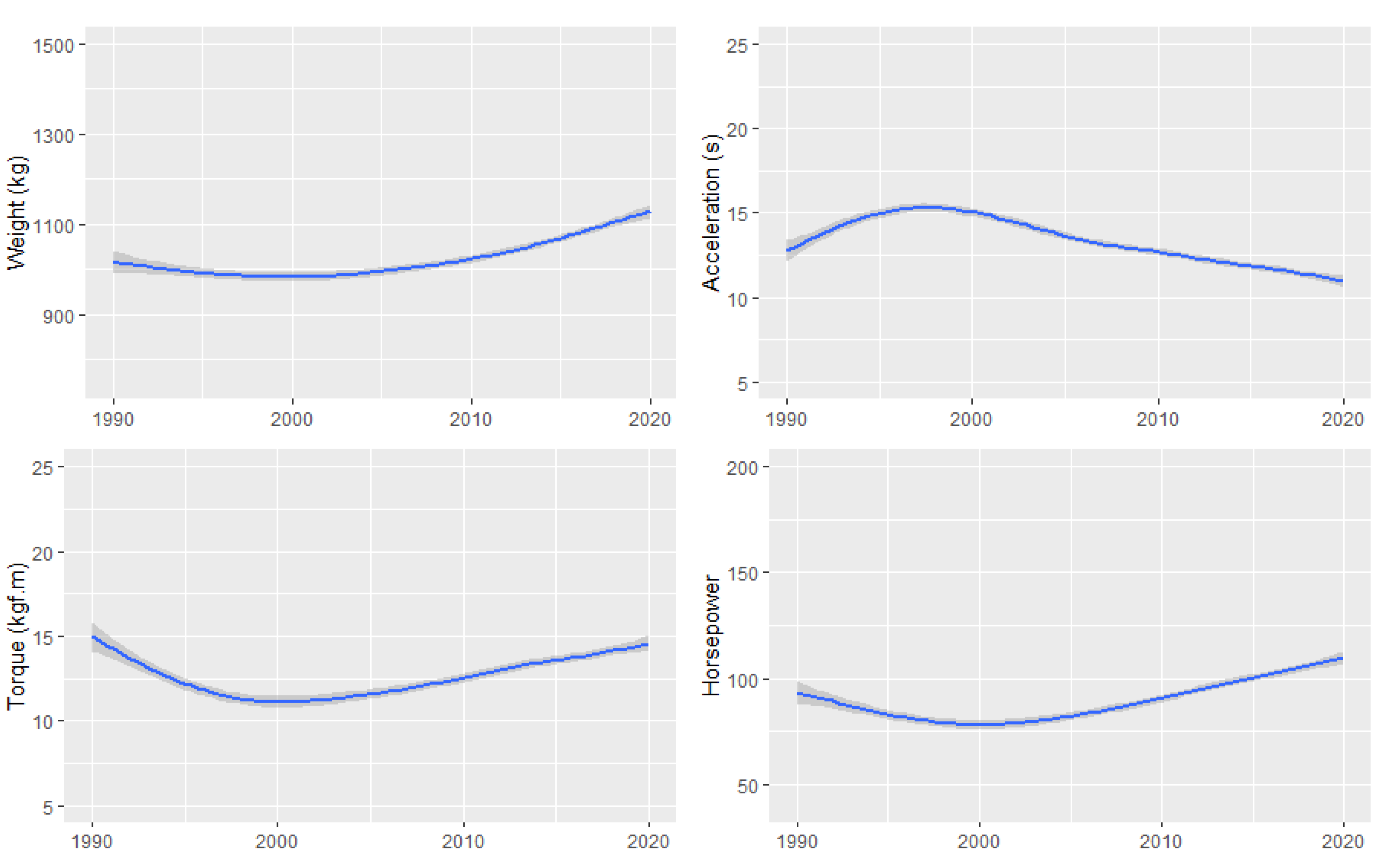
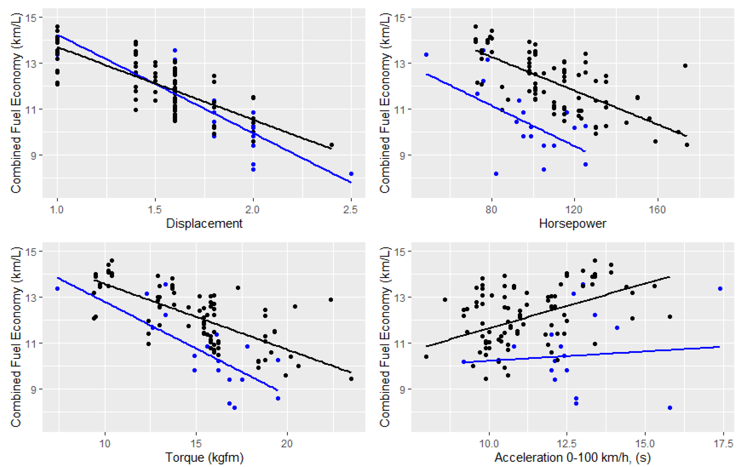
Figure 1a,b illustrates these tendencies for the Brazilian market. As with ton.mpg, these metrics will help dissect what happened to the LDV market in Brazil, although the method was not employed here. The P S F I for Brazil behaved better than ton.mpg. Apart from a slight dip in the beginning of the 1990s, the values increased constantly. Performance (P, in blue) reached a peak between 1993 and 1994, declined to a bottom in 1999, and then improved constantly. Herein, size (S, in purple) was measured, length × height × width, instead of interior volume, which decreased in the 1990s before increasing steadily. The FE (F, in red) decreased in this period, discussed in detail in Section 4, as the Brazilian market changed significantly.
Bandivadekar [31] further expanded on the rationale behind P S F I proposing the Emphasis on Reducing Fuel Consumption ( E R F C ) according to Equation (2). This simple concept allows the illustration of the magnitude of these trade-offs. A generic gasoline ICE 2035 model with 0% ERFC would see an increase in its power-to-weight ratio (HP/WT, in horsepower and lbs) from 0.059 to 0.087 (47.5%), with time to accelerate from 0 to 100 km/h reduced from 8.7 to 6.4 s while maintaining fuel consumption at 8.1 L/100 km. In contrast, if the power-to-weigh ratio and acceleration remained at 2008 levels (i.e., a 100% ERFC), FE would reach 5.5 L/100 km, which is a 47.3% reduction. From a GHG emissions perspective, a 35% reduction from a No Change scenario would be possible by 2035. However, “all current trends run counter to the required changes”. Note that E R F C does not need to stop at 100% as performance could reduce below baseline grades, thus reaching even more significant improvements in the FE.
E R F C = F C c u r r e n t F C r e a l i z e d F C c u r r e n t F C p o t e n t i a l
According to Mackenzie [4], there are two drawbacks to An and DeCicco’s approach. First, acceleration, and not the power-to-weight ratio, should be the preferred performance measure. Second, and most importantly, their approach assumes a 1:1:1 trade-off between size, power-to-weight ratio, and FE with no theoretical reason.
Knittel [3], which is extensively cited in this study, estimated that when all other parameters are equal, a 10% reduction in weight produced a 4.19% increase in FE. and a 10% increase in horsepower decreased FE by 2.62%. Thus, the 1:1:1 trade-off does not occur. Torque effects were not statistically significant. The econometric model used to reach these numbers is discussed in detail in Section 3. Another important conclusion was found: average FE could have increased by approximately 60% in the period 1980–2006 if vehicle attributes, such as weight, horsepower, and torque, were maintained at the 1980 levels. Actual realized improvements were 15%. This fact may raise questions about incentives to consumption trends, such as for household appliances [
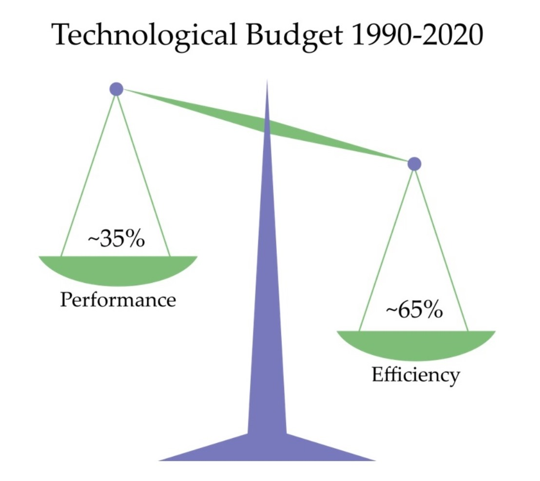
32]. Some of these are as follows: what kind of vehicles are suitable for urban, highway, and other different applications? Which policies may the exergy analysis contribute to the better end-use of exergy, considering technological gains and security parameters?
Mackenzie [4] followed this approach and modeled fuel consumption in gallons per mile (gpm) as a function of inertia weight (IWT) in kg, acceleration from 0 to 97 km/h (Z97), and other vehicle parameters. The authors used eight econometric models in their analyses and accounted for weight reductions that would have happened if not for changes in size, features, and functionality. This potential mass reduction was 650 kg or 40% for the average vehicle from 1975 to 2009 [33]. Additionally, they found that a 10% reduction in inertia weight resulted in a 6.9% decrease in fuel consumption for the same period. Furthermore, a 10% improvement in acceleration resulted in a 4.4% increase in fuel consumption without modifications in other variables. Moreover, it was estimated that per-mile fuel consumption could have been reduced by about 70% (3.4% per year) if not for improvements in acceleration, new features, and functionalities. The rate of technological progress was not uniform, averaging 5% and 2.1% per year during the periods 1975–1990 and 1990–2009, respectively.
Subsequently, an adapted version of Bandivadekar’s ERFC was used to calculate values for the period 1975–2009. The evolution follows a “V-shaped” curve, with ERFC exceeding 100% from 1975 to 1980 (when performance was reduced to increase efficiency), −25% in 1995–2000 (when performance improvements outpaced technological capability; thus, efficiency was reduced), before rebounding to 75% in 2005–2009 (a value between 0 and 1 implies both performance and efficiency improved simultaneously, but at compromised levels).
Hu and Chen [34] applied Knittel and Mackenzie’s method for the European market from 1975 to 2015. They found that the rates of technological progress were slightly lower than those in the USA. However, the most interesting finding was that engine size, weight, and power were actually reduced by 20%, 5%, and 2% respectively, from 2006 to 2015. Although torque and acceleration performance increased by 11% and 7%, respectively, these developments, combined with the increased penetration of diesel vehicles, increased FE by 32% in the period. This shift was also observed in the Swedish market, where 33% of technological development was used for improved FE in 1975–2007 and 77% in 2007–2010 [35]. Kwon [36] controlled the engine size for the Great Britain market from 1979 to 2000. FE improved by 0.9% per year but could have been 1.1% if not for the increased average engine capacity. Furthermore, performance offsetting better technological gains was observed in the Dutch market from 1990 to 1997 because of higher engine capacity and more weight [37]. J. Wu et al. [38] applied Knittel’s approach to the Chinese market from 2010 to 2019 and differentiated between indigenous, joint-venture, and foreign vehicle manufacturers. They found rates of yearly technological progress between 3.1% and 3.9%.
Drawbacks of this econometric approach are that it assumes constant elasticities and trade-offs for the entire period studied, which usually spans a few decades.This may not necessarily be the case, according to Moskalik [39]. By modeling individual engines, Moskalik found a general trend toward lower elasticity values for the trade-off between acceleration and fuel economy over time. This is because modern engines have broader efficiency islands. Another drawback is that this approach relies on FE from standardized tests, which could differ significantly from real-world conditions. Craglia and Cullen [40] used real-world FE data and further divided regression analysis on the basis of powertrain, petrol, diesel, and hybrid engines in Britain from 2001 to 2018. They found different elasticities for different powertrains by justifying the division. Additionally, they found that 60% of potential efficiency gains were offset by increasing size and power.

3. Methods

Knittel [3] empirically estimated the efficiency trade-offs and technological progress of the United States vehicle market by considering FE ( m p g ) as a function of attributes, such as weight ( w t ), horsepower ( h p ), torque ( t q ), and a vector of other vehicle characteristics X related to FE, for vehicle i in year t. A multiplicative term referred to as technological progress T, also called “year fixed effects”, and an average zero error term, ϵ , is expressed in Equation (3).
m p g i t = T t f ( w t i t , h p i t , t q i t , X i t , ϵ i t )
To apply the linear regression analysis, a natural logarithm is applied to both sides of (3), which results in the following.
ln m p g i t = T t + β 1 × ln w t i t + β 2 × ln h p i t + β 3 × ln t q i t + X i t × B + ϵ i t
Mackenzie [4] followed this approach. However, the fuel consumption was modeled in gallons per mile ( g p m ) as a function of inertia weight ( I W T ) in kg, acceleration (from 0 km/h to 97 km/h) (Z97) in seconds, interior volume ( V O L ) in m3, a vector of other vehicle characteristics X , and the mean zero error term ϵ , according to (5).
ln g p m i t = T t + β 1 × ln I W T i t + β 2 × ln Z 97 i t + β 3 × ln V O L i t + X i t × B + ϵ i t

Model Specifications

FE here was modeled as a function of vehicle weight and a term related to performance (either torque, horsepower or acceleration, in Models 1–3, respectively) and vector X , which includes dummy variables for the powertrain and gearbox. Applying the natural logarithm to Equation (3) yields Equation (6). The objective is to estimate technological advancements, including these covariates related to technology such as fuel injection or turbo-compressors, and this would result in underestimating the year-fixed effects as these features absorb technological improvements. If the objective is to estimate the effects of each of these technologies on FE, they should be included in the models. The first approach was preferred in this study.
ln k m l i t = T t + β 1 × ln w t i t + β 2 × ln p e r f o r m a n c e i t + X i t × B + ϵ i t
The discussion presented in Section 4.3 describes the trends relating horsepower, torque, and acceleration. They are highly correlated with engine displacement, which is the combined volume swept by all cylinders. Thus, three models, corresponding to each performance variable, were estimated.

4. Brazilian LDV Market Evolution

This section provides an overview of specific LDV parameters pertinent to the models used and to the sales-mix during the 1990–2020 period. Data visualization is performed before performing regression analysis, which helps in understanding trends and trade-offs.

4.1. Establishing Data-Set

For creating a data-set, some assumptions were made. There is no available data-set, such as the one provided by EPA for the USA, for Brazil. Since 2009, the Brazilian National Institute of Metrology Standardization and Industrial Quality (INMETRO) has been publishing FE (FE values in Brazil are regulated by two technical standards: ABNT NBR 6601 and 7024 for urban and highway cycles, respectively. They are based on cycles FTP-75 and HWFET provided by the EPA) and certain vehicle parametric data, such as engine displacement and transmission, for the labelling program of Brazil. Manufactures can choose the model data that they want to publish, and there is an overlap between categories, which are based on size [21]. However, crucial data, such as vehicle weight, is not available. Thus, a data-set was established using values from the website [41]. These values were checked for consistency and compared with the data obtained from specialized research magazines to the greatest extent.
Because the data-set was established without a reference, it was not possible to compile data from more than 10,000 models, which is generally the norm observed in existing studies. To best represent an actual fleet, the best-selling models, targeting approximately 75% to 80% of sales in that year, were selected. Thus, the established data-set reflects neither all models available in that particular year nor are sales weighted, but it is a compromise between both. Including low-selling, high-price models, which are inherently more technologically advanced, could bias the results upwards, inflating the rate of technological improvement, which would not be reflected in the streets. Using sales as a guide may allow the results to reflect shifts in market-share.
Generally, LDVs are not allowed to operate on diesel fuel. Therefore, vehicles using diesel fuel, such as light trucks, were not considered in this study. The established data-set consists of 2615 vehicles from 1990 to 2020. Since 2003, flex-fuel vehicles, which can operate on either ethanol or gasoline (by government decree, gasoline in Brazil has anhydrous ethanol mixed in it, with values fluctuating between 18% and 27.5% in volume) or a mixture of both, rapidly gained market share (approximately 90% of vehicle licensing). The FE values of ethanol in flex-fuel vehicles are not reported here because it would only double the amount of data presented. The average FE value for ethanol is 0.7 times that of gasoline owing to its lower heating value.
The R-environment and R-Studio [42] were used for data processing and analysis. Graphics were generated using the ggplot2 package [43]. The technical details and steps to perform the regression in R were obtained using [44].

4.2. Evolution of Key Parameters

The evolution of certain key parameters used in the regression analyses is illustrated here to understand their developments. As observed in Figure 2, FE undergoes three distinct phases. First, it improved from 1990 to 1998, then regressed slightly until 2004, and finally improved again.
Acceleration, horsepower, torque, and displacement are highly correlated; therefore, their trajectories exhibit resemblance. Average torque and horsepower initially decreased until 2003, and subsequently increased. Consequently, acceleration time initially increased from 1990 to 2002. However, it is currently below its value in 1990. Average weight (Figure 3 exhibited a stable trend until 2003; however, it is currently exhibiting an upward trend. This loss of power throughout the 1990s may be related to the mandatory inclusion of catalytic converters in 1997, which was already introduced in 1992, or the entry-level, compact, and low-powered popular gaining market share.

4.3. Performance Parameters and Fuel Economy

Both Knittel [3] and Mackenzie [4] used weight in regression analyses as one of the main explanatory variables influencing FE, and Figure 4 illustrates the reason for using weight. By keeping other parameters constant, a heavier car consumes more fuel than a lighter car. Values represented in blue are for the year 1990 and those in black are for 2018 (although analyses were performed until 2020, the results from 2018 were used in the figures as there are slightly greater number of vehicles in the data-set of 2018). A straight trend line was added for illustrative purposes. The trend line shifting up from 1990 to 2018 indicates that when all other parameters are equal, a vehicle with the same weight today has better FE owing to technological improvements.
Knittel [3] employed both horsepower and torque as performance variables, whereas Mackenzie [4] employed acceleration time, in seconds, required for a vehicle to reach a speed of 97 km/h from 0 km/h.
In addition, torque, horsepower, and acceleration were highly correlated with displacement, as shown in Figure 5a. A higher value of displacement indicates higher values of torque and horsepower, but a lower value of acceleration time. Knittel [3] justified the inclusion of both horsepower and torque in the same model as the maximum values occur under different RPMs. For the data-set established and used in this study, models employing both of these variables resulted in estimators with opposing signals, which should not ideally happen. Therefore, they were considered separately.
Here, Figure 6 illustrates that the above-mentioned parameters are highly correlated with fuel consumption. When all other parameters are equal, higher torque, higher horsepower, and lower acceleration time imply that the vehicle requires more energy. The blue and black lines represent the results in year 1990 and 2018, respectively. The curves exhibit an increasing trend from 1990 to 2018. This indicates the improvements in FE for the same performance. In the case of displacement, the lines are more ambiguous as specific power and torque per liter of cylinder displacement steadily increased in this period by 44% and 15.3%, respectively. This indicates that a 1.6 L engine in 2020 exhibits better performance than that of its 1990 counterpart. Although a typical 1.6 L engine in 1990–1992 generated approximately 77 HP and 13 kgfm of power and torque, respectively, these values increased to approximately 113 HP (+46.7%) and 15.8 kgfm (+21.5%), respectively, in 2018–2020 (there is no turbocharged 1.6 L engine in the data-set; otherwise, the average HP and torque would have been even higher).

4.4. Relative Sales Categories

Vehicle registration increased from approximately 500,000 units to more than 3,000,000 units in 2013 (there is no sales model available for the years 1999 and 2000. The values for 1998 are for January–May only). Furthermore, the market is diversifying; it is moving away from the subcompact, affordable vehicles and toward larger, heavier, and more powerful units [6]. The appearance of the SUV, compact or large, is observed. One can compare this scenario with the scenario in the USA, wherein the advent of the light truck increased the market share from less than 2% in 1975 to 49% in 2009 [33]. This had significant impacts on sales-weighted FE averages. Figure 7 illustrates this diversification and tendency toward larger vehicle categories. Subcompact and compact cars accounted for approximately 75% of total sales in 2004, and this ratio dropped to approximately 35% in 2020. Compact and large SUVs occupied a majority of this market share during this period. Although FE improved during this period in every category, it was slightly lower for the compact SUV model than for a compact vehicle, as will be examined in the following sections.
Since 2003, the LDVs sold in Brazil are capable of operating on gasoline, ethanol, or on a mixture of both. These flex-fuel vehicles (FFVs) enable higher flexibility in terms of fuel usage to the consumer. However, this flexibility comes at a cost as engines cannot be optimized for either fuel, which typically requires different compression ratios; for example, 12:1 for ethanol and 8:1 for gasoline. As compression ratio is directly correlated to maximum theoretical efficiency [6,45], the result exhibits a slight decrease in FE when compared to the dedicated-fuel engines. Regression models included this variable to capture its effect on FE.
As no official published data regarding the sales-weighted average FE for Brazil were available, these values were estimated by making some simplifications. First, the best sales models were selected, which represented approximately 75% of the total sales. Some models featured more than one engine; for example, featuring both 1.0 L and 1.6 L engines. However, the sales figures do not show such details. Thus, the FE values of all models that were available in the chosen year were averaged. In addition, only the values of highway FE were shown. On average, the urban FE value was approximately 82% of the highway FE value. This implies that the average FE for an urban drive is 0.82 × 13.6 = 11.5 km/L and that for a combined 55/45 cycle, it is is 12.0 km/L. Using the average FE values of every vehicle category from [23] along with the sales-mix data, the sales-weighted average FE for the combined cycle was obtained, which was 12.2 km/L.

5. Results and Discussion

5.1. Trade-Offs

Results of the regression models are listed in Table 1, with standard errors provided within parenthesis. A 10% decrease in weight resulted in a 3.59–4.70% increase in FE, which is in good agreement with the previously reported results. The effects of performance generated a 0.97% decrease in FE for every 10% increase in torque, 0.59% decrease in horsepower, and 0.79% decrease in acceleration (value is positive as the metric is the number of seconds required to reach 100 km/h from idle. Reducing this time requires more energy). Effects for transmission causes a slight decrease in FE for automatic transmission (AT) vehicles than that for manual transmission (MT) vehicles. CVT and DCT provide FE benefits, but they are equipped in more expensive models, with more advanced technology, such as in fuel injection and variable valve timing.
As expected, the hybrid and pure-electric vehicles have significant impacts on FE (60% and 100%, respectively). The slight positive effect of dedicated gasoline engines was expected, as discussed above.
Two bestselling, long-running models were used to illustrate trade-offs. A typical subcompact MY1990 exhibited an acceleration, horsepower, torque, weight, and combined FE of 17.4 s, 48.5 HP, 7.2 kgfm, 798 kg, and 13.4 km/L, respectively. In contrast, MY2020 exhibited 12.5 s (+39.2%), 72 HP (+48.5%), 10.4 kgfm (+44.4%), 1025 kg (+28.4%), and 14.0 km/L (+4.5%), respectively.
For a typical 1.6 L compact vehicle, the acceleration time decreased from 13.0 s to 9.8 s, (+32.6%), power increased from 76 HP to 101 HP (+32.9%), torque increased from 13.3 kgfm to 15.4 kgfm (+15.8%), weight increased from 872 kg to 1036 kg (+18.8%), and FE decreased from 13.5 km/L to 12.1 km/L (−10%). If the performance analyses were conducted at the 1990 levels, FE would have been 17.7 km/L and 17.8 km/L for the 1990 and 2000 models, respectively.
A family-sized sedan (MY1992) gained 20% in HP, 33.5% in torque, and 10% in acceleration owing to the increase in engine displacement from 1.6 L to 2.0 L. It further gained 24.6% in weight when CVT replaced MT, whereas FE remained almost constant (11.4 km/L (1.6 L) vs. 11.5 km/L (2.0 L)).
As reducing weight is associated with improvements in FE, vehicle downsizing (Engine downsizing usually refers to reducing displacement and adding turbocharging to keep performance constant. Vehicle downsizing simply means making it smaller and lighter) is considered for reducing fuel consumption in the fleet. However, this implies that the trend of vehicles becoming larger and heavier, as shown in Figure 3 and discussed above, has to be reversed. There are a few more models in the data-set with 15 or more years on the market, and in none of them has weight or power reductions occurred, which is quite the opposite. Moreover, this is not taking into account that weight-saving technologies were probably employed in the period [4]. The same can be said for vehicle categories, all of which are more powerful and heavier.

5.2. Technological Progress

The logarithmic values of FE obtained from the year 2020 are 0.2607, 0.2825, and 0.2835 times greater than those from the year 1990 for Models 1–3, respectively. This translates to 29.8%, 32.6%, and 32.8% progress, respectively, or roughly 1.0% per year. These rates of progress are analogous to those observed in the P S F I index in Figure 1a. Table 2 summarizes the rates of technological progress for each year during 1991–2020 (1990 being equal to zero) and for each model. These rates are uneven in the period considered, approximately 0.39–0.61%, 0.85–0.89%, and 1.7–1.9% during 1990–2000, 2001–2010, and 2011–2020, respectively. The lower rates in the 1990s may be related to electronic injection systems replacing carburetors. The former operates with stoichiometric mixtures, whereas carburetors operates on lean mixtures. This causes slight reduction in efficiency. In 2012, the Brazilian government set guidelines for mandatory FE improvements of at least 12.08% by the year 2017 compared to that in 2011 (INOVAR-AUTO program). This was observed to have a positive effect on the rates, which improved to approximately 3% recently.
The overall rate of improvement was lower than that observed in the studies discussed above, which is usually at least 3%. The reasons may be that the Brazilian market was traditionally dominated by cheaper models, with inherently lower technological levels. Higher rates were observed during the period when the market started to diversify. Weiss et al. [46] applied the same method for model variants of the EU Volkswagen Golf, Opel Astra, and Ford Focus, considered compact vehicles in the EU. FE could be 23% higher in 2018 compared to 1980 if mass, power, and frontal area remained at the 1980 levels; thus, an 0.6% increase per year.
Furthermore, a hypothetical average FE value for year t can be obtained by multiplying the average FE of year 0 with the exponential of the difference between parameters T t and T 0 , according to (7).
ln k m l t ln k m l 0 = T t T 0 k m l t = k m l 0 × e ( T t T 0 )
The average combined FE values (across all models; not sales-weighted) in 1990 and 2020 were 10.43 km/L and 12.43 km/L, respectively, which indicates a 19.2% increase by 2020. The potential FE values in 2020, by applying the rates of technological progress according to Table 2, would be 13.36 km/L, 13.74 km/L, and 13.76 km/L. Thus, the E R F C values are, according to Equation (2), 69%, 61%, and 61%. This implies that approximately 31–39% of technological progress was spent in performance during the entire period.

6. The Future

The energy consumption variables of future transport are complex, such as energy production technology, economic and population growth, customer demands, industrial policy, air quality, alternative fuels, and technology trends [7]. Transport in 2020 is 99.8% powered by ICEs, with approximately 1.1 billion LDVs, a number that is expected to reach 1.7–2.0 billion in 2040. Even with the rapid expansion of alternative fuel vehicles (AFVs), it is expected that approximately 85–90% of transport energy will be obtained from liquid fuels powering ICEs [47]. This section presents a few possible pathways in technological progress rates and sales-mix evolution, including EVs. This enables building scenarios for fleet-wide FEs in 2030 and 2035, which are presented in Section 7.

6.1. Internal Combustion Engines

As discussed above, ICEs will still be the major prime movers for decades to come, regardless of AFVs penetration, because alternatives have to start from very low bases [7]. ICEs can still benefit from newer technologies and increase their efficiency and performance. Although no attempt is made here to discuss all possible future technologies, a brief discussion to illustrate these possible gains in efficiency is provided.
Improvements can be in the form of over-expanded cycles, such as the Atkinson and Miller cycles [48,49] replacing the traditional Otto cycle. Other areas of technological improvement include gasoline direct injection (GDI) with lean combustion, variable compression ratio, water injection, cylinder deactivation, external exhaust gas re-circulation (EGR), and multi-stage air charging [50]. Furthermore, GDI compression–ignition [51] can allow ICES to reach the efficiency levels of HEVs. Moreover, engines can be downsized and turbocharged to improve efficiency [52].
Middleton et al. [53,54] simulated the economic implications of technologies, from the perspectives of FE, in a baseline MY2012 Ford Fusion midsize sedan. The technologies included in their study were dual cam phasing, discrete variable valve lift (DVVL), engine friction reduction, GDI, downsizing with boosters, cooled EGR, and reductions in weight, drag and rolling resistances. By combining these technologies, fuel consumption could reduce by 35%, from 31.8 MPG to 48.8 MPG in the 55/45 cycle.

6.2. Electrification

Electrification of transport is one of the most common solutions suggested when the topic of mitigation of GHG emissions arise. Battery electric vehicles (BEVs) rely only on electricity. Their main concerns are the battery capacity, weight, cost, range, charging infrastructure, and emissions associated with power generation. In contrast, HEVs employ a combination of an ICE and electric motor. The latter may be used for powering short trips. When the battery range is exhausted, the battery is recharged using the ICE. A plug-in hybrid electric vehicle (PHEV) combines the advantages of both HEV and BEV, wherein the battery can be recharged with an appropriated power outlet. A mild hybrid electric vehicle (MHEV) allows its engine to be turned off while idling and may employ regenerative breaking, which recovers some energy that would otherwise be lost while braking. Electric mobility uptake may be improved by educating citizens about their advantages, such as environmental, economic and quality of life [55]. It is important to understand the specifics needs of each country as conducted by [12,14].
As discussed above, higher performance and sales-mix shifts could offset these technical gains partially or totally. The same could happen in the case of EVs. According to Galvin [56], EVs are still less powerful than ICEs in the US (254 HP vs. 284 HP on average); however, this gap may be closed by the emergence of super-powerful EVs, with power greater than 600 HP. It was estimated that a 5% increase in the weight of the smaller EVs results in a 4.7% increase in electricity demand, whereas for larger EVs, the increase is 10.5%. The latter gaining market-share would exert greater pressure on the rate of de-carbonization of electricity generation. While these findings should be kept in mind, this exercise in shifting EV market share is not attempted here, as this would create yet another layer of complexity. Thus, EVs here are employed in a somewhat optimistic light. EVs energy consumption are depended on travel time, distance and external temperature, but these refinements are not pursued here. Also not considered are the car-sharing services, which can play an important role in total energy consumption [57].
Some authors indicate the necessity of proper car-hailing and human mobility [58,59]; moreover, they show the need for policymakers to understand the specific characteristics of each kind of transportation toward a cleaner mobility sector. Another article [55] used the concept of “electric mobility education” to improve the effect and depth of the information and learning technologies, which is the basis for all policymakers.

6.3. Efficiency Pathways

The results listed in Table 2 suggests about 30% efficiency improvement in 30 years, or 1% per year. With an ERFC of approximately 60%, FE improved by 0.6% per year. Development was considerably uneven; accumulated improvements reached 10% only in 2007 or 2008. Thus, six scenarios were selected, from 0.0% to 3.0% yearly improvement with 0.5% increments. Recently, an improvement of 3% was observed. However, this would require maintaining constant performance, which is unlikely to happen for prolonged periods. An improvement of 0% does not necessarily imply zero technological progress. It indicates that all technological improvements were used for improving the performance. This scenario is slightly less unlikely. Every rate between 0% and 3% may indicate a combination of a specific rate of technological progress and ERFC between 0 and 1. Exploring every combination of these two factors is unnecessary as these scenarios are of the “what if?” nature.
The Brazilian government instituted a target of 11% reduction in sales-weighted fleet FC by 2022 compared to that in 2017. FC in 2017 was 1.75 MJ/km, and the target was 1.55 MJ/km. This translates to a 2.4% reduction in FC per year. These values were adjusted for real-world conditions, thereby resulting in lower values. The adjusted values were 2.46 MJ/km and 2.18 MJ/km, respectively. With the official E22 heating value at 28.99 MJ/L, FE should be 11.8 km/L in 2017. Applying a rate of improvement of 2.4% per year, FE values in 2030 and 2035 would be 16.2 km/L and 18.3 km/L, respectively. These values are used as references for the scenarios presented in the subsequent sections.

6.4. Establishing Baselines

To estimate possible efficiency pathways, first, it is necessary to establish a baseline. This is achieved by simplifying the actual fleet to correspond with a few representative models and dividing according to the vehicle category, as listed in Table 3, which further summarizes the market share during the years 2020 and 2001. These values were based on two different data-sets. The term sales-mix refers to the 50 best selling vehicles, which account for 88% of total registrations. FE values were obtained from [23], which contained 1034 models. FE values were not sales-weighted and corresponded to the combined 55/45 cycle. Extra-large (the size of Ford Fusion is categorized as an extra-large vehicle in Brazil, as opposed to it being in the mid-size category in the USA), off-road, and sports cars were discarded due to their negligible number of sales.

6.5. Sales-Mix

Shift in sales-mix is an important and often neglected aspect. Therefore, four scenarios were created to explore this aspect. The first scenario is called SUV, wherein compact and full-size SUVs attain 40% and 50% combined market share in 2030 and 2035 (continuing their recent trends). The second scenario combines subcompact and compact vehicles, corresponding to 70% and 80% market share in 2030 and 2035, respectively; herein, they reach and subsequently exceed the values observed in 2001. xEVs in both cases are 5% and 10% in 2030 and 2035, respectively.
The Brazilian National Association of Vehicle Manufacturers (ANFAVEA) partnered with the Boston Consulting Group (BCG) [60] to create two scenarios (Table 4) for the market penetration of hybrid and electric vehicles—xEVs (this term is used to refer to PHEVs, BEVs, HEVs, and MHEVs)—in Brazil for the years 2030 and 2035. The “Inertial” scenario projects aim for 12% and 32% xEVs market share in 2030 and 2035, respectively, whereas the “Global Convergence” scenario projects aim for 22% and 62%. With estimated rate of fleet turnover, xEVs are expected to make 2–4% of the fleet in 2030 and 10–18% in 2035. For simplification purposes, xEVs were considered HEV and BE.

7. Fe Scenarios in 2030 and 2035—Policy Implications

Results in Table 5 and Table 6 are for the sales-weighted FE in the 55/45 cycle. The baseline sales-weighted average FE was 12.2 km/L in 2020, as discussed in Section 4.4. Values for yearly technological improvements in both tables are in percentage. Values in bold indicate that they exceed 16.2 km/L and 18.3 km/L in 2030 and 2035, respectively, as discussed in Section 6.3. To obtain these values, the rate of technological improvement should exceed the values observed in the last decade, i.e., 1.7–1.9%. However, the estimated average values from 2017 to 2020 were 3–3.1%. If performance continues to improve at such historical rates, consuming approximately 31–39% of technological improvements, a 4% yearly rate would be needed. Shifting toward smaller, more fuel efficient, and compact xEVs would require a smaller rate of improvement as these categories are inherently more efficient.
Moreover, extreme scenarios produce extreme results. If 62% of the new vehicles sold in 2035 are xEVs, combined with 3% yearly improvements in FE, the average FE would more than double to 28.2 km/L. The likelihood of the fleet FE doubling in 15 years is low. According to the EPA, FE increased from approximately 12.5 MPG to 25 MPG in 45 years (1975 to 2020) in the USA.
However, if the compact and full-size SUVs continue to gain market share and all efficiency gains are used for performance, the average FE would reach 12.3 km/L and 12.6 km/L, and the xEVs market share in this scenario would be 5% and 10% in 2030 and 2035, respectively. This indicates that the higher efficiency of xEVs would be almost completely offset by the shift in sales toward larger and less efficient ICE vehicle categories. However, this is not likely to happen as ERFC would remain at 0% for an extended period.
Conversely, if sales were to be shifted toward subcompact and compact, i.e., to the 2001 levels (70% combined) and beyond (80% in 2035), then FE would actually be higher than its value in the moderate xEV scenario in 2030 and approximately 4% lower in 2035. Making this shift toward smaller, less powerful vehicles would possibly require a combination of factors. Vehicles today are subject to different taxes according to their displacement capacity. With engines producing more power per displacement over time, this taxation could move toward weight and horsepower.
These FE values should not be taken as forecasting but merely to translate into numbers some possible developments. Fleet FE could remain stagnant for years, if Brazilians show preference towards performance and size, and xEVs fail to penetrate the fleet in any significant manner. Dramatic FE improvements could be realized if efficiency is completely prioritized over performance.
The policy implications are that regulations can help steer toward higher fleet FE. Recently, the rate of technological improvements increased owing to the government instituting mandatory FE improvements. These mandates were revised and will be in place for another decade, but targets could be updated every five years. Recent targets are 2.4% improvements in fleet FE per year. Although this rate is higher than those observed thus far, it is still lower than those observed recently in China, or in the USA and Europe.

7.1. The Road Not Taken

If this study was focused on estimating the total GHG emissions, the following values would be required: (i) Total fleet per year; (ii) vehicle age distribution per year; (iii) kilometers travelled per vehicle, per age; (iv) possible rate of increase in kilometers travelled per year, per vehicle; (v) fuel sales-mix of ethanol and gasoline; (vi) average GHG emissions for producing electricity used in xEVs; (vii) possible difference in marginal rate of GHG emissions for accommodating the increasing demands for electricity for the xEVs; (viii) sales-mix per vehicle category; and (ix) average FE per vehicle category.
The average FE, as discussed above, can be varied by two or more factors. For other key variables listed above, the same possibilities exist. Holistic projections of such nature would require major assumptions/simplifications, which compound uncertainty as more variables are being considered. What this article attempted was to shed light on the evolution of some important variables: historical rates of technological improvement, trade-off between performance and efficiency, and shifts in vehicle sales-mix.

8. Conclusions and Policy Implications

Rates of technological progress were estimated for the LDV fleet in Brazil from 1990 to 2020. These rates were lower than the rates observed in the developed countries; however, improvements were observed, from approximately 0.39% to 0.61%, 0.85% to 0.89%, and 1.7% to 1.9% in successive decades. Not all of this progress was used for improving FE, approximately 31–39% was offset by better performance, defined by weight and power in this study. This trade-off between efficiency and performance has major implications as it directly affects fleet-wide fuel efficiency.
Furthermore, shifts in market share play an important role as heavier vehicles require more energy, which were estimated using regression models. In Brazil, the traditional compact and subcompact vehicles are gradually being replaced by compact and full-size SUVs. Another observation is that LDVs in Brazil are becoming bigger, heavier, and more powerful over time in every vehicle category. Thus, scenarios that consider vehicle downsizing, constant performance (or even regressing), and sales shifting toward smaller models must acknowledge that a reversal of trends would be necessary.
These rates of technological progress along with sales-mix shifts in favor of SUVs, compacts, or xEVs were explored under various scenarios for the years 2030 and 2035. Sales-weighted fleet-wide FE can range between 12.3 km/L and 18.3 km/L in 2030 and between 12.6 km/L and 28.2 km/L in 2035. This variability reflects the effects of the main factors studied here, including technological improvements, trade-offs, and sales-mix, on FE. If the market shifts toward heavier and more powerful vehicles and manufactures expend all technological progress to improve performance, FE would remain stagnant for years. However, if the rate of technological progress continues to improve and is geared completely toward achieving higher efficiency, combined with the market shifting toward xEVs, then FE can more than double compared to baseline in 15 years. These results were used to assess the feasibility of the recent government program for improving FE, with the mandated rates being reached in the last few years. However, these rates are already observed in other countries, such as the USA and China.
Limitations of this study include the data-set used for analyses, which was not as extensive as those used in similar studies. Although the values reported were statistically significant, and a more comprehensive data-set may not alter the study results significantly, more data could aid in conducting a more detailed analysis, such as estimating if elasticities varied yearly or can be considered constant. Furthermore, an extensive data-set could be used to obtain regressions for different power-trains, such as hybrids or electric vehicles. As discussed above, there are still significant gaps in our knowledge about the Brazilian fleet, and this research provided helpful figures, such as feasible rates of technological progress. These can be used to estimate better possible GHG emissions in the future, which is the ultimate research goal.

Author Contributions

Conceptualization, R.F.M. and C.E.K.M.; Formal analysis, R.F.M.; Methodology, R.F.M.; Supervision, C.E.K.M. All authors have read and agreed to the published version of the manuscript.

Funding

This study was supported by the National Council for the Improvement of Higher Education (CAPES), and the CNPq (Brazilian National Council for Scientific and Technological Development) (grant numbers 307405/2021-4, 304395/2018-8, and 400401/2016-9), and FAPESP (São Paulo Research Foundation) (grant number 2015/22883-7).

Institutional Review Board Statement

Not applicable.

Informed Consent Statement

Not applicable.

Data Availability Statement

Not applicable.

Conflicts of Interest

The authors declare no conflict of interest.

References

  1. de Pesquisa Energética, E. Brazilian Energy Balance 2020: Year 2019; EPE: Rio de Janeiro, Brazil, 2020. [Google Scholar]
  2. Greene, D.L.; Sims, C.B.; Muratori, M. Two trillion gallons: Fuel savings from fuel economy improvements to US light-duty vehicles, 1975–2018. Energy Policy 2020, 142, 111517. [Google Scholar] [CrossRef]
  3. Knittel, C.R. Automobiles on steroids: Product attribute trade-offs and technological progress in the automobile sector. Am. Econ. Rev. 2011, 101, 3368–3399. [Google Scholar] [CrossRef] [Green Version]
  4. MacKenzie, D.W. Fuel Economy Regulations and Efficiency Technology Improvements in US Cars Since 1975. Ph.D. Thesis, Massachusetts Institute of Technology, Cambridge, MA, USA, 2013. [Google Scholar]
  5. Larrick, R.P.; Soll, J.B. The MPG illusion. Science 2008, 320, 1593–1594. [Google Scholar] [CrossRef] [PubMed]
  6. Mosquim, R.F.; Mady, C.E.K. Design, performance trends, and exergy efficiency of the Brazilian passenger vehicle fleet: 1970–2020. J. Clean. Prod. 2021, 290, 125788. [Google Scholar] [CrossRef]
  7. Kalghatgi, G. Is it really the end of internal combustion engines and petroleum in transport? Appl. Energy 2018, 225, 965–974. [Google Scholar] [CrossRef]
  8. Falco, D.G.; Sacilotto, L.M.; Cavaliero, C.K.N. Urban Collective Mobility: Global Challenges Toward Sustainability. In Environmental Sustainability; CRC Press: Boca Raton, FL, USA, 2021; pp. 272–291. [Google Scholar]
  9. Malaquias, A.C.T.; Netto, N.A.D.; da Costa, R.B.R.; Langeani, M.; Baêta, J.G.C. The misleading total replacement of internal combustion engines by electric motors and a study of the Brazilian ethanol importance for the sustainable future of mobility: A review. J. Braz. Soc. Mech. Sci. Eng. 2019, 41, 1–23. [Google Scholar] [CrossRef]
  10. Nogueira, G.P.; McManus, M.C.; Leak, D.J.; Franco, T.T.; de Souza Dias, M.O.; Cavaliero, C.K.N. Are eucalyptus harvest residues a truly burden-free biomass source for bioenergy? A deeper look into biorefinery process design and Life Cycle Assessment. J. Clean. Prod. 2021, 299, 126956. [Google Scholar] [CrossRef]
  11. Velandia Vargas, J.E.; Seabra, J.E.; Cavaliero, C.K.; Walter, A.; Souza, S.P.; Falco, D.G. The new neighbor across the street: An outlook for battery electric vehicles adoption in Brazil. World Electr. Veh. J. 2020, 11, 60. [Google Scholar] [CrossRef]
  12. Tomanik, E.; Policarpo, E.; Rovai, F. Life Cycle Assessment of Vehicular Electrification; Technical Report; SAE Technical Paper; SAE: Warrendale, PA, USA, 2022. [Google Scholar]
  13. Ferrari, F.; Nogueira, G.; Franco, T.; Dias, M.; Cavaliero, C.; Witkamp, G.J.; Van Der Wielen, L.; Forte, M.B.S. The role of ionic liquid pretreatment and recycling design in the sustainability of a biorefinery: A sugarcane to ethanol example. Green Chem. 2021, 23, 9126–9139. [Google Scholar] [CrossRef]
  14. He, X.; Zhang, S.; Wu, Y.; Wallington, T.J.; Lu, X.; Tamor, M.A.; McElroy, M.B.; Zhang, K.M.; Nielsen, C.P.; Hao, J. Economic and climate benefits of electric vehicles in China, the United States, and Germany. Environ. Sci. Technol. 2019, 53, 11013–11022. [Google Scholar] [CrossRef] [PubMed]
  15. Cheah, L.; Evans, C.; Bandivadekar, A.; Heywood, J. Factor of two: Halving the fuel consumption of new US automobiles by 2035. In Reducing Climate Impacts in the Transportation Sector; Springer: Berlin/Heidelberg, Germany, 2008; pp. 49–71. [Google Scholar]
  16. Highlights of the Automotive Trends Report. Available online: https://www.epa.gov/automotive-trends/highlights-automotive-trends-report (accessed on 18 April 2022).
  17. Schmitt, W.F.; Szklo, A.; Schaeffer, R. Policies for improving the efficiency of the Brazilian light-duty vehicle fleet and their implications for fuel use, greenhouse gas emissions and land use. Energy Policy 2011, 39, 3163–3176. [Google Scholar] [CrossRef]
  18. Benvenutti, L.M.; Uriona-Maldonado, M.; Campos, L.M. The impact of CO2 mitigation policies on light vehicle fleet in Brazil. Energy Policy 2019, 126, 370–379. [Google Scholar]
  19. Benvenutti, L.M.M.; Ribeiro, A.B.; Uriona, M. Long term diffusion dynamics of alternative fuel vehicles in Brazil. J. Clean. Prod. 2017, 164, 1571–1585. [Google Scholar] [CrossRef]
  20. De Melo, C.A.; Jannuzzi, G.D.M.; Santana, P.H.D.M. Why should Brazil to implement mandatory fuel economy standards for the light vehicle fleet? Renew. Sustain. Energy Rev. 2018, 81, 1166–1174. [Google Scholar] [CrossRef]
  21. Smith, C.B. Análise da Difusão de Novas Tecnologias Automotivas em prol da Eficiência Energética na Frota de Novos Veículos Leves no Brasil. Ph.D. Thesis, Universidade Federal do Rio de Janeiro, Rio de Janeiro, Brazil, 2010. [Google Scholar]
  22. Bastin, C.; Szklo, A.; Rosa, L.P. Diffusion of new automotive technologies for improving energy efficiency in Brazil’s light vehicle fleet. Energy Policy 2010, 38, 3586–3597. [Google Scholar] [CrossRef]
  23. INMETRO. Programa Brasileiro de Etiquetagem. Available online: http://pbeveicular.petrobras.com.br (accessed on 24 July 2020).
  24. Wills, W.; La Rovere, E.L. Light vehicle energy efficiency programs and their impact on Brazilian CO2 emissions. Energy Policy 2010, 38, 6453–6462. [Google Scholar] [CrossRef]
  25. Sistema de Estimativas de Emissões e Remoções de Gases de Efeito Estufa (SEEG). Available online: https://plataforma.seeg.eco.br/sectors/energia (accessed on 19 April 2022).
  26. de Andrade Junior, M.A.U.; Valin, H.; Soterroni, A.C.; Ramos, F.M.; Halog, A. Exploring future scenarios of ethanol demand in Brazil and their land-use implications. Energy Policy 2019, 134, 110958. [Google Scholar] [CrossRef] [Green Version]
  27. de Salvo Junior, O.; de Almeida, F.G.V. Influence of technologies on energy efficiency results of official Brazilian tests of vehicle energy consumption. Appl. Energy 2019, 241, 98–112. [Google Scholar]
  28. de Salvo Junior, O.; de Souza, M.T.S.; de Almeida, F.G.V. Implementation of new technologies for reducing fuel consumption of automobiles in Brazil according to the Brazilian Vehicle Labelling Programme. Energy 2021, 233, 121132. [Google Scholar] [CrossRef]
  29. Lutsey, N.; Sperling, D. Energy efficiency, fuel economy, and policy implications. Transp. Res. Rec. 2005, 1941, 8–17. [Google Scholar] [CrossRef]
  30. An, F.; DeCicco, J. Trends in technical efficiency trade-offs for the US light vehicle fleet. SAE Trans. 2007, 116, 859–873. [Google Scholar]
  31. Bandivadekar, A.P. Evaluating the Impact of Advanced Vehicle and Fuel Technologies in US Light Duty Vehicle Fleet. Ph.D. Thesis, Massachusetts Institute of Technology, Engineering Systems Division, Cambridge, MA, USA, 2008. [Google Scholar]
  32. Keutenedjian Mady, C.E.; Reis Pinto, C.; Torelli Reis Martins Pereira, M. Application of the second law of thermodynamics in brazilian residential appliances towards a rational use of energy. Entropy 2020, 22, 616. [Google Scholar] [CrossRef]
  33. Cheah, L.W. Cars on a Diet: The Material and Energy Impacts of Passenger Vehicle Weight Reduction in the US. Ph.D. Thesis, Massachusetts Institute of Technology, Cambridge, MA, USA, 2010. [Google Scholar]
  34. Hu, K.; Chen, Y. Technological growth of fuel efficiency in european automobile market 1975–2015. Energy Policy 2016, 98, 142–148. [Google Scholar] [CrossRef] [Green Version]
  35. Sprei, F.; Karlsson, S. Energy efficiency versus gains in consumer amenities—An example from new cars sold in Sweden. Energy Policy 2013, 53, 490–499. [Google Scholar] [CrossRef]
  36. Kwon, T.H. The determinants of the changes in car fuel efficiency in Great Britain (1978–2000). Energy Policy 2006, 34, 2405–2412. [Google Scholar] [CrossRef]
  37. Van den Brink, R.M.; Van Wee, B. Why has car-fleet specific fuel consumption not shown any decrease since 1990? Quantitative analysis of Dutch passenger car-fleet specific fuel consumption. Transp. Res. Part D Transp. Environ. 2001, 6, 75–93. [Google Scholar] [CrossRef]
  38. Wu, J.; Posen, I.D.; MacLean, H.L. Trade-offs between vehicle fuel economy and performance: Evidence from heterogeneous firms in China. Energy Policy 2021, 156, 112445. [Google Scholar] [CrossRef]
  39. Moskalik, A.; Newman, K. Assessment of Changing Relationships between Vehicle Fuel Consumption and Acceleration Performance; Technical Report; SAE Technical Paper; SAE: Warrendale, PA, USA, 2020. [Google Scholar]
  40. Craglia, M.; Cullen, J. Do technical improvements lead to real efficiency gains? Disaggregating changes in transport energy intensity. Energy Policy 2019, 134, 110991. [Google Scholar] [CrossRef]
  41. Carrosnaweb. 2020. Available online: http://www.carrosnaweb.com.br (accessed on 1 December 2019).
  42. R Core Team. R: A Language and Environment for Statistical Computing; R Foundation for Statistical Computing: Vienna, Austria, 2017. [Google Scholar]
  43. Wickham, H. ggplot2: Elegant Graphics for Data Analysis; Springer: New York, NY, USA, 2009. [Google Scholar]
  44. Hanck, C.; Arnold, M.; Gerber, A.; Schmelzer, M. Introduction to Econometrics with R; University of Duisburg-Essen: Duisburg, Germany, 2019. [Google Scholar]
  45. Serrenho, A.C.; Sousa, T.; Warr, B.; Ayres, R.U.; Domingos, T. Decomposition of useful work intensity: The EU (European Union)-15 countries from 1960 to 2009. Energy 2014, 76, 704–715. [Google Scholar] [CrossRef]
  46. Weiss, M.; Irrgang, L.; Kiefer, A.T.; Roth, J.R.; Helmers, E. Mass-and power-related efficiency trade-offs and CO2 emissions of compact passenger cars. J. Clean. Prod. 2020, 243, 118326. [Google Scholar] [CrossRef]
  47. Leach, F.; Kalghatgi, G.; Stone, R.; Miles, P. The scope for improving the efficiency and environmental impact of internal combustion engines. Transp. Eng. 2020, 1, 100005. [Google Scholar] [CrossRef]
  48. Naber, J.D.; Johnson, J.E. Internal combustion engine cycles and concepts. In Alternative Fuels and Advanced Vehicle Technologies for Improved Environmental Performance; Elsevier: Amsterdam, The Netherlands, 2014; pp. 197–224. [Google Scholar]
  49. Toda, T.; Sakai, M. The New Toyota Inline 4-Cylinder 2.5 L Gasoline Engine; Technical Report; SAE Technical Paper; SAE: Warrendale, PA, USA, 2017. [Google Scholar]
  50. De Cesare, M.; Cavina, N.; Paiano, L. Technology comparison for spark ignition engines of new generation. SAE Int. J. Engines 2017, 10, 2513–2534. [Google Scholar] [CrossRef]
  51. Sellnau, M.; Foster, M.; Moore, W.; Sinnamon, J.; Hoyer, K.; Klemm, W. Pathway to 50% brake thermal efficiency using gasoline direct injection compression ignition. SAE Int. J. Adv. Curr. Pract. Mobil. 2019, 1, 1581–1603. [Google Scholar]
  52. Jono, M.; Taguchi, M.; Shonohara, T.; Narihiro, S. Development of a New 2.0 L I4 Turbocharged Gasoline Direct Injection Engine; Technical Report; SAE Technical Paper; SAE: Warrendale, PA, USA, 2016. [Google Scholar]
  53. Middleton, R.J.; Gupta, O.G.H.; Chang, H.Y.; Lavoie, G.; Martz, J. Fuel Efficiency Estimates for Future Light Duty Vehicles, Part A: Engine Technology and Efficiency; Technical Report; SAE Technical Paper; SAE: Warrendale, PA, USA, 2016. [Google Scholar]
  54. Middleton, R.J.; Harihara Gupta, O.G.; Chang, H.Y.; Lavoie, G.; Martz, J. Fuel Efficiency Estimates for Future Light Duty Vehicles, Part B: Powertrain Technology and Drive Cycle Fuel Economy; Technical Report; SAE Technical Paper; SAE: Warrendale, PA, USA, 2016. [Google Scholar]
  55. Turoń, K.; Kubik, A.; Chen, F. When, What and How to Teach about Electric Mobility? An Innovative Teaching Concept for All Stages of Education: Lessons from Poland. Energies 2021, 14, 6440. [Google Scholar] [CrossRef]
  56. Galvin, R. Are electric vehicles getting too big and heavy? Modelling future vehicle journeying demand on a decarbonized US electricity grid. Energy Policy 2022, 161, 112746. [Google Scholar] [CrossRef]
  57. Turoń, K.; Kubik, A.; Chen, F. Operational aspects of electric vehicles from car-sharing systems. Energies 2019, 12, 4614. [Google Scholar] [CrossRef] [Green Version]
  58. Zeng, I.Y.; Chen, J.; Niu, Z.; Liu, Q.; Wu, T. The GHG Emissions Assessment of Online Car-Hailing Development under the Intervention of Evaluation Policies in China. Sustainability 2022, 14, 1908. [Google Scholar] [CrossRef]
  59. Li, Y.; Yang, Y.; Luo, G.; Huang, J.; Wu, T. The Economic Recovery from Traffic Restriction Policies during the COVID-19 through the Perspective of Regional Differences and Sustainable Development: Based on Human Mobility Data in China. Sustainability 2022, 14, 6453. [Google Scholar] [CrossRef]
  60. O Caminho da Descarbonização do Setor Automotivo no Brasil. Available online: https://acervo.anfavea.com.br/AcervoDocs/APRESENTA%C3%87%C3%83O_ANFAVEA_E_BCG.pdf (accessed on 20 April 2022).
Figure 1. P S F I and its parameters for the Brazilian LDV market, 1990 to 2020, adapted from [30]. (a) An and DeCicco’s P S F I for Brazil, 1990 to 2020. (b) P, S, and F for Brazil, 1990 to 2020.
Energies 15 05416 g001
Figure 2. Combined FE in Brazilian transportation sector from 1990 to 2020 (horizontal axis).
Energies 15 05416 g002
Figure 3. Evolution of key LDV parameters used in the regression models from 1990 to 2020 (horizontal axis).
Energies 15 05416 g003
Figure 4. FE vs. weight (1990 in blue and 2018 in black).
Energies 15 05416 g004
Figure 5. Torque, horsepower, and acceleration as a function of displacement. (a) Acceleration vs. Horsepower; (b) Torque vs. Horsepower.
Energies 15 05416 g005
Figure 6. Performance parameters and FE (1990 in blue and 2018 in black).
Energies 15 05416 g006
Figure 7. Vehicle registration categories from 1990 to 2020 (horizontal axis).
Energies 15 05416 g007
Table 1. Regression results for FE, where models 1, 2, and 3 indicate the elasticity of each explanatory variable, bearing in mind that torque, horsepower, and acceleration are linearly dependent.
Model 1Model 2Model 3
Weight−0.359 ***−0.423 ***−0.470 ***
(0.023)(0.025)(0.018)
Torque−0.097 ***--
(0.010)
Horsepower-−0.059 ***-
(0.012)
Acceleration--0.079 ***
(0.011)
Electric-vehicle1.076 ***1.045 ***1.062 ***
(0.033)(0.034)(0.033)
Gasoline0.042 ***0.046 ***0.041 ***
(0.010)(0.010)(0.010)
Hybrid0.571 ***0.569 ***0.581 ***
(0.016)(0.016)(0.016)
AT−0.003−0.004−0.010 **
(0.005)(0.005)(0.005)
CVT0.0070.0110.002
(0.010)(0.011)(0.011)
DCT0.348 ***0.328 ***0.319 ***
(0.087)(0.088)(0.088)
Constant5.047 ***5.487 ***5.353 ***
(0.141)(0.138)(0.137)
Observations262126222622
R20.6010.5900.593
Adjusted R20.5950.5840.587
Note: ** p < 0.05; *** p < 0.01.
Table 2. Accumulated rates of technological progress estimated for Models 1–3 (Percentage).
YearModel 1Model 2Model 3
19911.71.31.2
19920.90.90.8
19933.33.93.7
19943.23.73.6
19956.37.16.8
19966.16.86.9
19976.47.57.5
19986.97.97.9
19998.09.59.5
20005.67.37.3
20013.65.35.1
20020.42.02.0
20033.34.84.8
20045.57.07.0
20055.16.56.4
20068.210.210.0
20078.510.510.4
200811.713.913.6
200911.213.413.0
201012.114.213.8
201112.414.514.2
201212.915.014.8
201315.317.417.3
201415.818.318.0
201517.820.220.3
201618.020.420.6
201722.324.925.0
201826.128.728.9
201925.928.728.7
202029.832.632.8
Table 3. Baseline.
Table 3. Baseline.
Category2020 avg. FE2020 Market Share2001 Market Share
Subcompact13.84.023.8
Compact13.029.144.5
Mid-size13.122.819.0
Large11.44.12.5
Compact SUV11.520.6
SUV9.63.60.4
Compact Truck11.29.64.3
Truck (Diesel)9.75.13.2
Table 4. Sales-mix scenarios.
ScenarioxEV I xEV II SUV CPT
Year20302035203020352030203520302035
Subcompact0000002530
Compact201015515104550
Mid-size15101352020153
Large55555431
Cpt. SUV28202510354000
Full-size SUV585551000
Cpt. Truck101010510343
Truck55535333
xEV12322262510510
Table 5. 2030 FE scenarios.
Scenario3.02.52.01.51.00.50.0
SUV16.415.614.914.113.512.812.3
xEV I17.116.315.514.814.113.412.8
CPT17.917.016.215.514.714.013.4
xEV II18.317.516.615.815.114.313.7
Table 6. 2035 FE scenarios.
Scenario3.02.52.01.51.00.50.0
SUV19.618.216.915.714.613.612.6
xEV I22.420.819.418.016.715.514.4
CPT21.519.918.617.316.014.913.8
xEV II28.126.124.322.621.019.518.3
Publisher’s Note: MDPI stays neutral with regard to jurisdictional claims in published maps and institutional affiliations.

