A Novel Coordination Mechanism for Connected and Automated Vehicles in the Multi-Intersection Road Network

Abstract

In recent years, connected automated vehicles (CAVs) have attracted much attention, and the coordination strategy of CAVs in isolated intersections has been widely discussed. However, these algorithms for isolated intersections cannot be directly applied in a multi-intersection road network (MiRN). The coordination strategy in the MiRN requires further investigation. This paper proposes a two-tier strategy for CAV coordination in the MiRN. First, we analyze the coordination problem in isolated intersections and formulate it as a mixed-integer programming problem. Then, for the MiRN, we propose a consensus prediction method to estimate the travel time for CAVs with different paths. Finally, a novel coordination approach is given, showing how to determine the optimal path for CAVs. The experimental results demonstrate the efficiency of the proposed strategy under various traffic flow rates. Compared with the fixed signal time assignment method and the actuated signal time assignment method, our method reduces the average travel time by about 74–83% under different flow rates. We also evaluate the impact of parameters on the strategy’s performance and provide some suggestions for setting these parameters.

1. Introduction

Globally, 55% of the world’s population resided in urban areas in 2018, which was forecasted to increase to 68% by 2050 [1]. However, the growing population in urban areas, without a corresponding increase in road capacity, results in traffic congestion. Traffic congestion grew persistently from 1982 to 2019 in U.S. urban areas [2]. To address the grand challenges urbanization brings, the “smart city” has become a ubiquitous concept, attracting increasing attention from academia, industry, and government [3]. Many major cities, such as Amsterdam, Zurich, Berlin, Singapore, New York, Beijing, etc., have established smart city initiatives or projects [4].

Smart mobility is an essential paradigm within the smart city concept, setting the foundation for various urban activities. The intelligent transportation system (ITS) is considered one of the primary building blocks of any smart city [5]. The ITS widely utilizes information and communications technology (ICT) to improve mobility, alleviate traffic congestion, and enrich and enhance urban services [6]. Next-generation ITS technologies, such as connected and automated vehicles (CAVs), are finishing their last phase toward large-scale worldwide deployment [7]. A CAV is supposed to be a vehicle capable of fulfilling the operational functions of a conventional vehicle on its own and of communicating with nearby vehicles and infrastructures for safer driving [8]. Studies show that about 94% of traffic accidents are related to driver behaviors, such as the driver’s cognitive errors, poor decision making, and improper handling [9]. CAVs can perceive the environment and react more quickly than humans through their advanced sensors and controllers, reducing the likelihood of collisions in the transportation system. This makes CAVs a feasible option for solving the current traffic problems [10,11]. The CAV is going to revolutionize the movement of people and goods; it is more than the automated car itself; it is a connected and automated system. Its existence dramatically depends on ITS technologies, including transport telematics, intelligent vehicles and infrastructures, and traffic control and coordination strategies.

For transport telematics, new technologies, such as IoT, Wi-Fi, 5G, and 6G, provide reliable support for vehicle-to-vehicle (V2V) communication to ensure its safety and real-time performance. Agarwal discussed V2V communication based on IoT and highlighted the Li-Fi technologies used in V2V communication systems [12]. Ezenwa emphasized that V2V communication is crucial for exchanging data seamlessly and securely between traffic participants via Wi-Fi (Wlan) or 4G/5G. He suggested that the DSRC technology is a viable solution due to its demonstrated capacity for safety-critical applications [13]. Shah K. et al. presented a survey on the adoption of BlockChain (BC) technology in the underlying 6G communication of IoVs. They discussed various privacy and security concerns in IoVs, which can be addressed via BC technology [14].

For intelligent vehicles and infrastructures, the research on vehicle construction, the control system for vehicles, and the safety guarantee system make the CAV a possible option in solving the current traffic problems in the future. The Society of Automotive Engineers (SAE) defined six levels of vehicle automation, from Level 0 (no automation) to Level 5 (full automation), which were adopted by the NHTSA and USDOT in 2016 [15]. Levels 1–3 require a driver to operate the vehicle with a license, whereas Levels 4–5 allow driverless operations. Companies have implemented Level 4 pilot projects to test AVs under certain circumstances, such as specific road types, areas, and weather. For example, Waymo and Uber evaluated driverless taxis in Phoenix and Arizona in 2017 [16,17]. For the vehicle infrastructures, C. Dong et al. proposed an Intelligent Vehicle Infrastructure Cooperative System (IVICS), based on Zigbee, which contained a roadside unit and an on-board unit [18]. J Gao et al. discussed the risk prevention methods for commercial vehicles based on intelligent vehicle and infrastructure systems. They summarized the prevention functions, which included Forward Vehicle Collision Warning (FCW), Advanced Emergency Braking (AEBS), and roll control [19]. Chu W. et al. investigated the concept of the cloud control system from cloud-related applications for intelligent and connected vehicles, as well as cloud control system architecture designing and its core technology development [20]. Molina et al. proposed a design strategy used at the architecture design level of autonomous vehicles that may facilitate the development, analysis, and, consequently, safety level assurance [21].

For traffic control and strategies in ITS, many scholars focused on strategies for merging traffic flows and traffic light management. Hari et al. proposed a novel approach to increasing the traffic flow near divergences, weavings, and bottlenecks with a mixed traffic of human-driven vehicles (HDVs) and CAVs. Their strategies can lead to an increase in throughput by several percent, thereby decreasing delays significantly [22]. Tachet et al. proposed a slot-based strategy for making traffic decisions, and it reasonably utilized adaptive vehicle platooning [23]. Mahhub A. et al. proposed a novel computational framework for real-time control to optimize energy consumption with the associated benefits. In addition, it works in corridors, including on-ramp merging, a speed reduction zone, and a roundabout [24]. Jiang Z. et al. proposed a two-stage CAV trajectory optimization strategy to improve fuel economy and reduce delays through a joint framework. They employed Pontryagin’s minimum principle (PMP) to smooth the vehicle trajectory under the vehicle dynamics and safety requirements. They designed a targeted method to avoid driving backward and to ensure an optimal vehicle gap [25]. Lei Chai and V. Garg et al. tried to generate traffic light signals to minimize congestion. Their solutions can detect congestion online and can consider the cumulative sum of the weights corresponding to vehicles on the road lanes to determine the time duration for each phase [26,27].

In the past decade, scholars have studied many relevant topics about ITS, including transport telematics, intelligent vehicles and infrastructures, and traffic control and coordination strategies. These works have made the CAV a viable solution that can alleviate traffic pressure and ensure safety. However, the research mentioned above only works in intersections with traffic lights. It still needs more work and remains challenging in signal-free intersections.

The previous cooperative driving research in signal-free intersections has focused on isolated intersections [28,29,30,31,32,33,34,35,36,37]. Based on different algorithms, such as the reservation scheme method [28,29,30], game theory [31,32], and the heuristic methods [33,34,35,36,37], different coordinative strategies have been proposed for the scene of isolated intersections. However, many isolated intersection algorithms cannot be directly applied to multi-intersection road networks because they lack optimal path selection for CAVs. This paper discusses how to deal with the optimal path selection problem and proposes a novel two-tier coordination strategy for CAVs passing through the multi-intersection road network (MiRN) efficiently and safely.

The coordination strategies for CAVs within the MiRN appear promising but remain challenging. Saber et al. and Chin et al. tried to find traffic signal optimization within the MiRN using machine learning methods [38,39]. However, their work does not work at signal-free intersections. Pei et al. proposed a distributed coordination driving strategy that decomposes the problem into small-scale sub-problems [39]. However, they assumed that CAVs drove along the trajectory given before the algorithm was triggered and did not explore the problem of optimal path selection. Wang et al. investigated the optimal path selection and proposed a complete traffic organization method for CAVs in MiRNs [40,41]. However, their approach only selected the shortest paths as candidate paths. Although more than one shortest path with the same path length may exist, the shortest path length is not necessarily the shortest travel time.

This paper proposes a novel coordination strategy for CAVs in the MiRN. First, we find the possible optimal paths for the CAVs from their origins to their destinations using the k-shortest paths algorithm. Next, we evaluate the time consumption of all possible paths using the average delays of all intersections within each path. Finally, we propose a comprehensive central control coordination strategy. The main contributions of this paper are as follows:

• We provide a complete coordination mechanism for CAVs passing through the MiRN to minimize their traveling time;
• We develop a consensus prediction method to estimate the travel time of CAVs with different paths and propose a new strategy to solve the optimal path selection problem.

The paper is organized as follows. Section 2 gives the description of the problem. Section 3 discusses the coordination strategy for CAVs in the MiRN in detail. Then, we provide the simulation results in Section 4. Finally, the conclusion and further works are presented in Section 5.

2. Problem Formulation

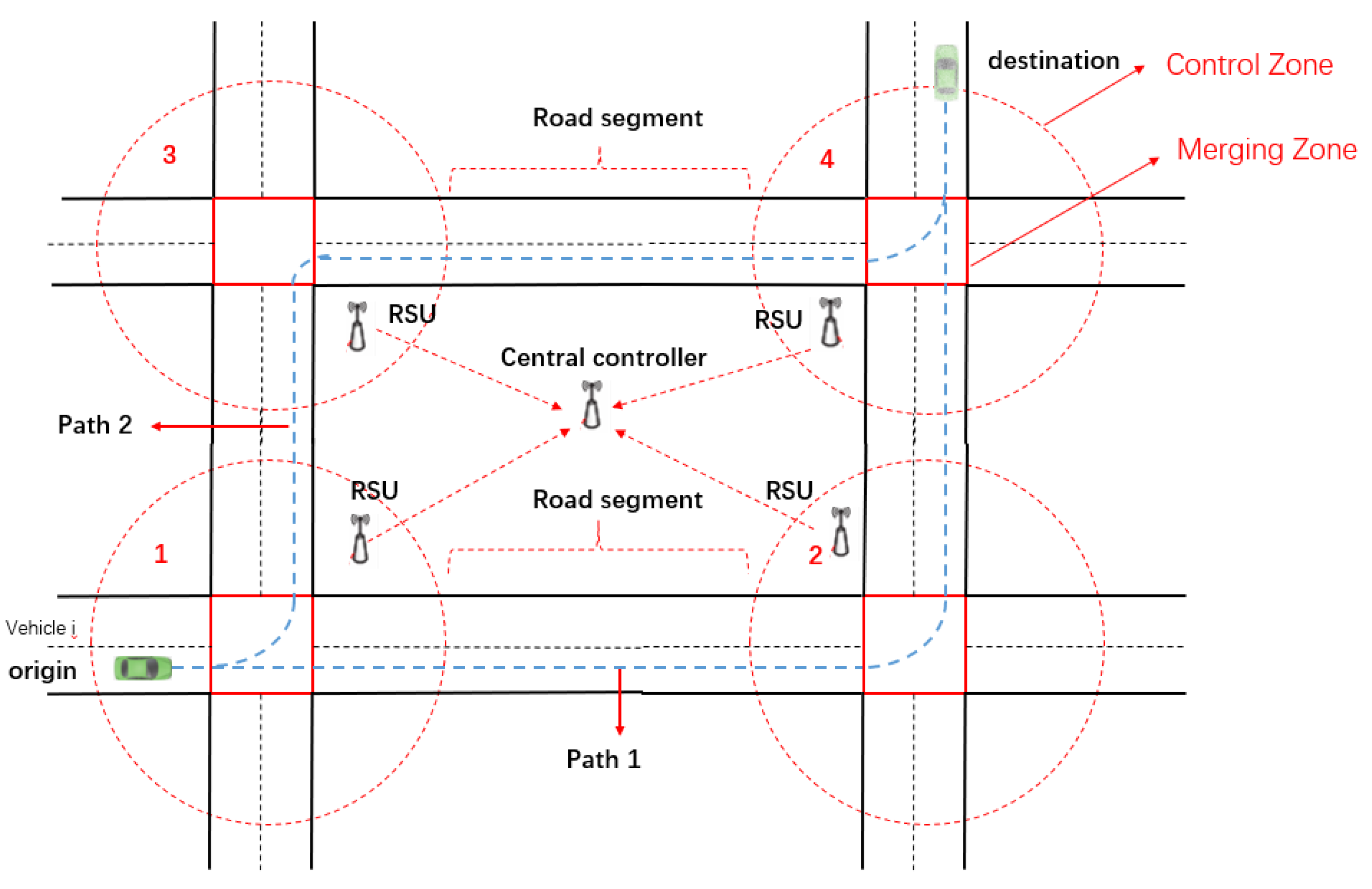
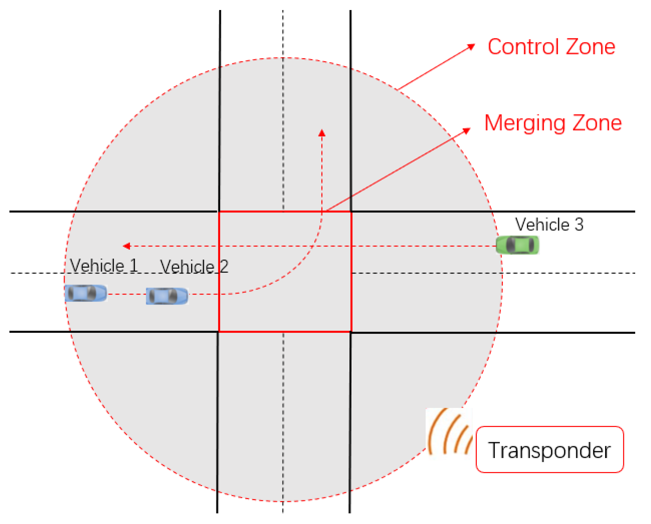
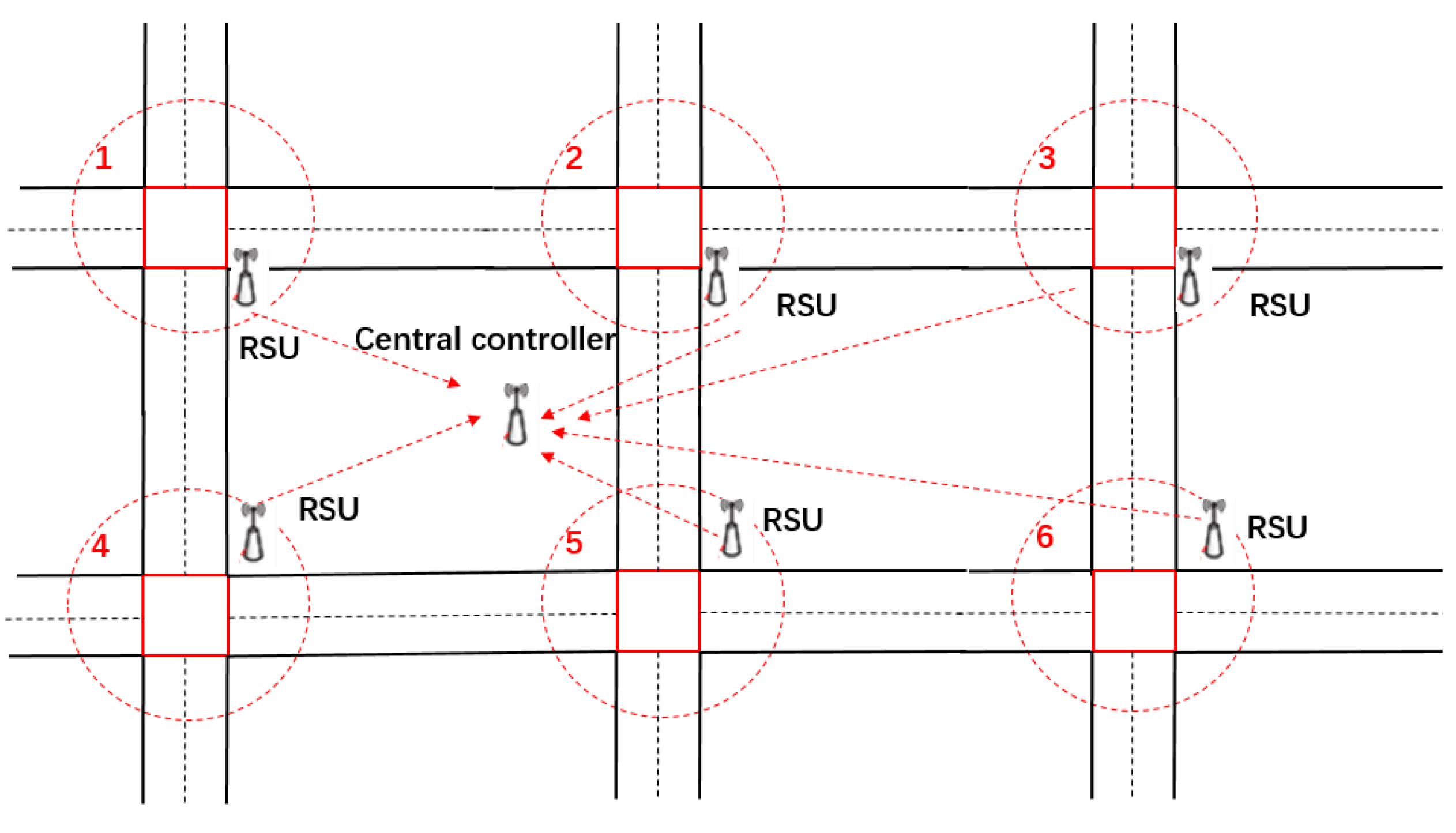
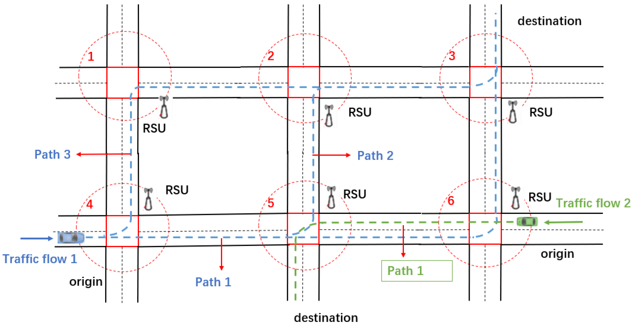
2.1. Scenario, Assumptions, and Notations

In this paper, we take a typical road network with four signal-free intersections as an illustration to explain our method, which is shown in Figure 1. We divide the area around the isolated intersection into the following two sections: the Control Zone (CZ) and the Merging Zone (MZ). The Control Zone is the circular area around the intersection where we can control the movement of the vehicles to avoid collisions. The Merging Zone is where the vehicles congregate. A roadside unit (RSU) is assigned as the local controller to schedule the CAVs within the intersection and exchange information with the central controller for each isolated intersection. Let $\mathrm{I}$ represent the set of intersections index, $\mathrm{I}=\left\{1,2,3,4\right\}$. There are multiple feasible paths for the CAVs in the MiRN, from their origins to their destinations. The coordination strategy aims to find the optimal path with minimum travel time and to let the CAVs pass each isolated intersection without collision.

Furthermore, several assumptions are made as follows:

• All vehicles in the network are CAVs;
• Once the path for a CAV has been determined, lane changes are not permitted.
• The CAVs move with a constant velocity $v_c$ outside intersections.

The main notations introduced in this paper are summarized in

Table 1. Main notations in this paper.

Notations	Meaning
$\mathrm{d}>0$	the width of each lane
$\mathrm{L}>0$	the distance from the entrance of the CZ
$\mathrm{l},\mathrm{w}>0$	the length and width of each vehicle
$v_{min},v_{max}>0$	the minimum and maximum speed
$a_{min}<0,a_{max}>0$	the minimum and maximum acceleration
$p_i\left(t\right)\in ℝ$	the position of the middle of vehicle $i$
$v_i\left(t\right)\in ℝ$	the speed of vehicle $i$
$t_i^{*}$	the time when vehicle $i$ enters MZ
$t_i^{min}$	the minimal time when vehicle $i$ enters MZ
$L_i$	the path set for vehicle $i$ from origin to destination
$h_{ik}$	one of the paths for vehicle $i$ from its origin to destination
$T_{i,h_{ik}}^1$	the time consumed in the road segment within the path $h_k$
$T_{i,h_{ik}}^2$	the delay time passing intersections within the path $h_k$
$t_{i,j}^{*}$	the assigned arrival time of vehicle $i$ in intersection $j$
$T_{j,t}^{*}$	the average delay in isolated intersection $j$ at time t
$C_{j,t}$	the set of CAVs in the intersection $j$ at time $t$
$t_{i,k}^{min}$	the minimal arrival time of vehicle $i$ to reach intersection k
$D_i$	the candidate path set for the vehicle i
T	the cycle time of exchanging information
M	the percent of rerouting CAVs
K	the number of the candidate path

.

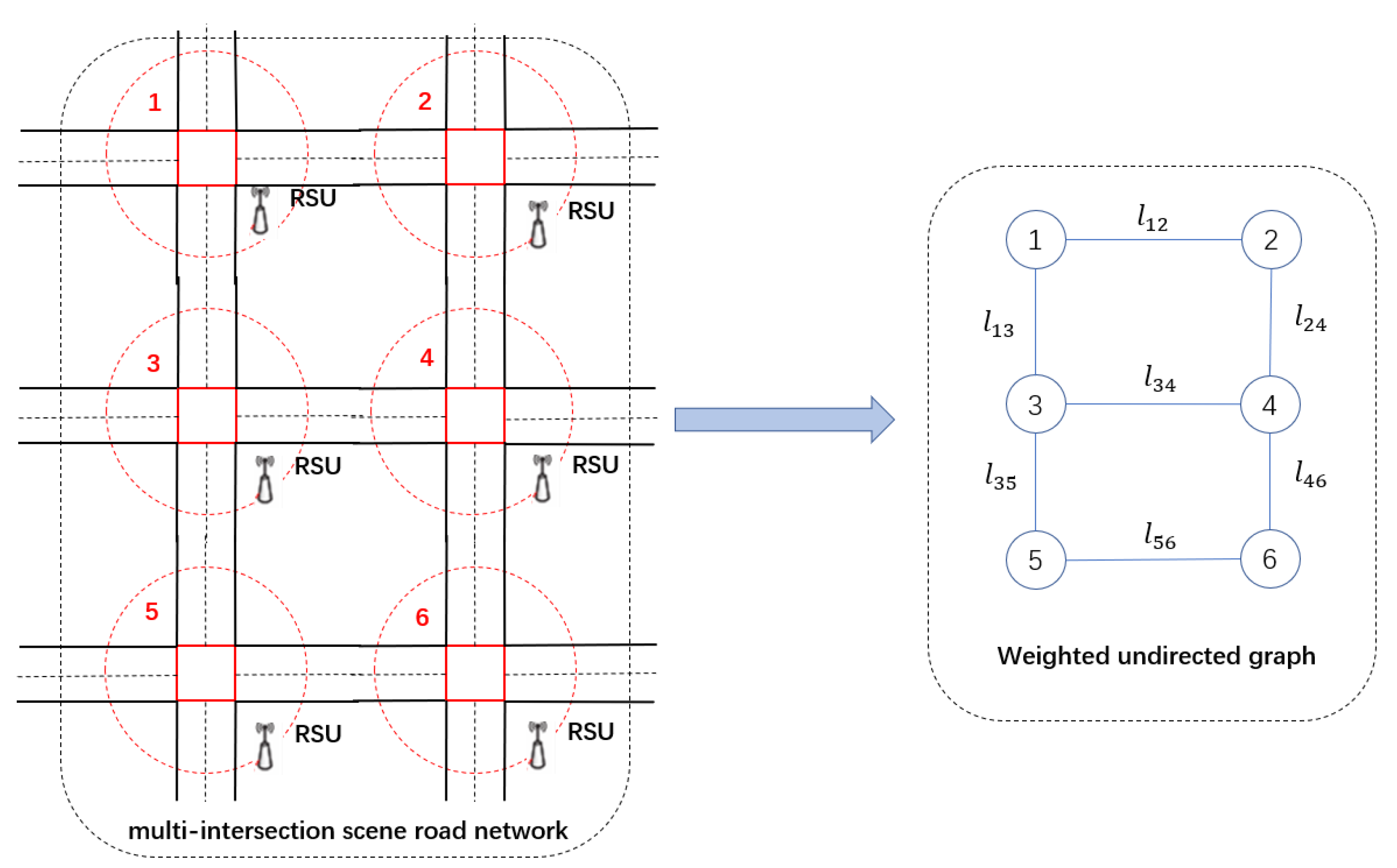
2.2. Path Planning Problem in the Road Network

To minimize the time of the vehicles passing through the MiRN, we must address two key issues. First, we choose the optimal paths for the CAVs with their corresponding origins and destinations. Different paths cost the CAVs different travel times and affect the traffic of the intersections in reverse. Second, we need to make the CAVs travel safely to avoid lateral and rear-end collisions.

The coordination strategy for the CAVs in the road network is a two-tier one. The central controller selects the optimal path for the CAVs to minimize the travel time. The RSU in each intersection is responsible for coordinating the CAVs to pass through each intersection safely and efficiently.

The MiRN can be described as a weighted, undirected graph, as shown in Figure 2. The weight $l_{j_1{j}_2},j_1,j_2\in I$ in the undirected graph represents the path length between intersections $j_1$ and $j_2$. For vehicle $i$, we use $o_i$ and $d_i$ to represent its origin and destination in the road network and $L_i$ to denote the feasible path set from $o_i$ to $d_i$, i.e., $L_i=\left\{h_{ik},k\ge 1\right\}$, where $h_{ik}$ is one of the possible paths.

The total travel time for a CAV includes the time spent on the road segments and intersections along the selected path. Let $T_{i,h_{ik}}^1$ stand for the time vehicle $i$ travels in the road segment and $T_{i,h_{ik}}^2$ denote the time for vehicle $i$ passing each isolated intersection, respectively, as:

$$T_{i,h_k}^1=\frac{dis(h_{ik})}{v_c},$$

(1)

$$T_{i,h_k}^2={\sum }_{j\in h_k}(t_{i,j}^{*}-t_{i,j}^{min}),$$

(2)

where $dis\left(h_{ik}\right)$ denotes the length of the feasible path $h_{ik}$ and j denotes the number of intersections within the path $h_{ik}$; $t_{i,j}^{*}$ is the assigned arrival time of vehicle $i$ in intersection $j$ and $t_{i,j}^{min}$ denotes the minimal arrival time of vehicle $i$ to reach the MZ area in intersection $j$.

The objective of the path planning for a CAV in the MiRN can be described as follows:

$$\begin{array}{l}\min \frac{dis\left(h_{ik}\right)}{v_c}+{{\displaystyle \sum }}_{j\in h_k}(t_{i,j}^{*}-t_{i,j}^{min}),\\ \hspace{1em}\mathrm{subject}\mathrm{to}:h_{ik}\in L_i\mathrm{and}\mathrm{safety}\mathrm{constraints}.\end{array}$$

(3)

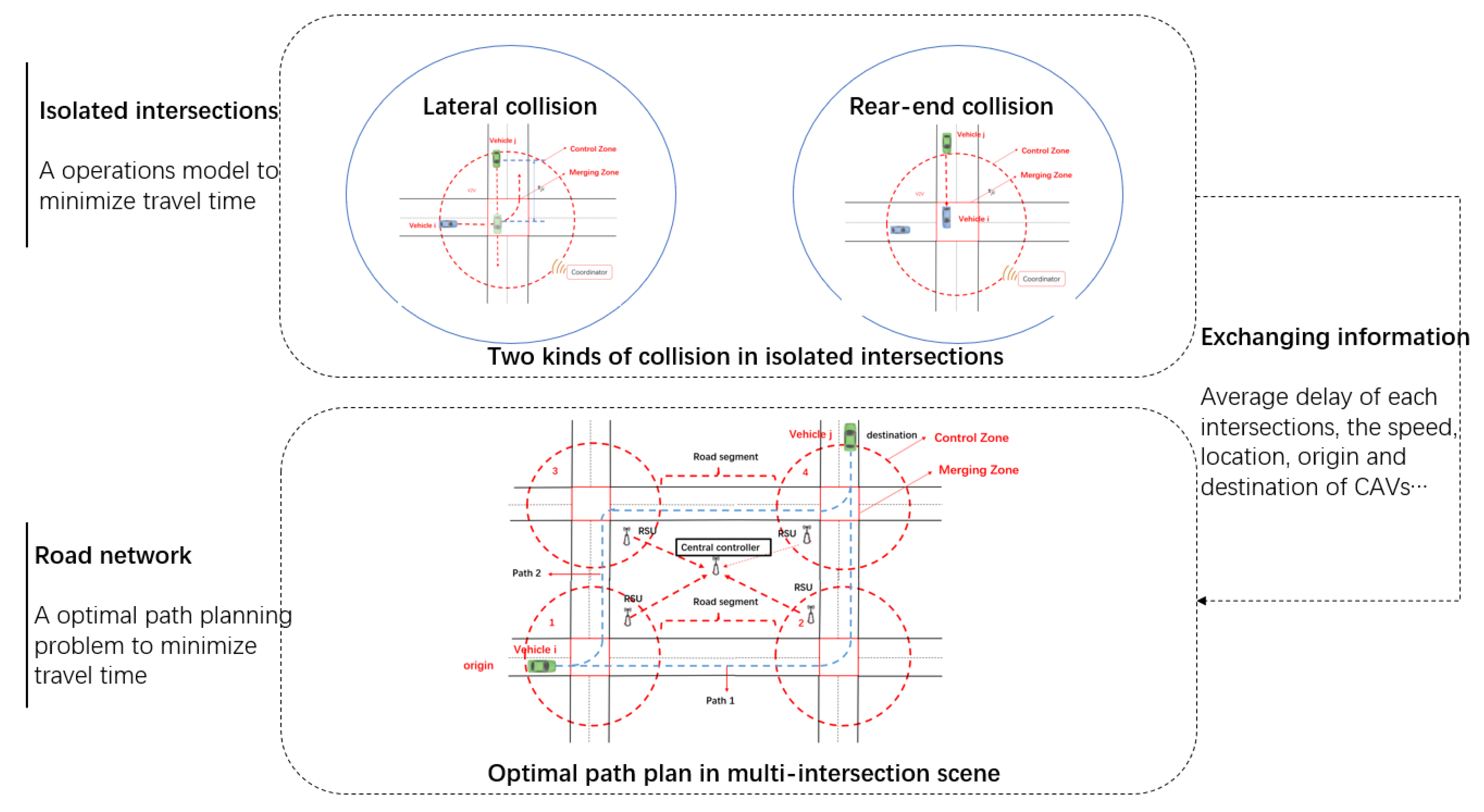
2.3. Constraints for CAVs in an Isolated Intersection

As is shown in Figure 3, there are two kinds of collisions for CAVs in isolated intersections. Lateral collisions are possible when vehicles traveling in different lanes pass through the MZ zone, such as vehicle 2 and vehicle 3. The rear-end collision happens when vehicles travel in the same lane, such as vehicles 1 and 2.

The coordination of the CAVs in the isolated intersection can be divided into two phases [32,34]. Firstly, we must optimize the sequence of the CAVs; then, we need to compute the trajectories in reverse, based on the sequence of the CAVs.

To formulate the problem from the view of the operational research, we introduce decision variables and constraints as follows:

• Decision variables: to decide the sequence of the CAVs, we define a binary variable $b_{ij}$ for each pair of CAVs that has a potential collision risk. If $b_{ij}=1$, vehicle $i$ has priority over vehicle $j$ to pass the intersections and vice versa;
• Lateral collision constraints: to avoid the lateral collision of the CAVs, $t_i^{*}$ represents the time when vehicle $i$ reaches the MZ area, $t_{safe}$ denotes the safe time interval, and M is a positive and sufficiently large number [40]; the constraints for avoiding lateral collisions can thus be written as:

  $$t_i^{*}-t_j^{*}+M\times b_{ij}\ge t_{safe},$$

  (4)

  $$t_j^{*}-t_i^{*}+M\times (1-b_{ij})\ge t_{safe}.$$

  (5)
• Rear-end collision constraints: for constraints of rear-end collision, let $f\left(i\right)$ represent the vehicle immediately preceding vehicle i in the same lane; $p_i\left(t\right)$ denotes the location of vehicle $i$ at time t, $\delta$ denotes the safety distance, and $l$ denotes the length of the vehicle. The constraints can be expressed as:

  $$p_{f(i)}(t)-p_i(t)\ge \delta +l.$$

  (6)
• Acceleration and speed constraints: furthermore, the longitudinal acceleration and speed should be within acceptable ranges as follows:

  $$a_{\min }\le {\dot{v}}_i(t)\le a_{\max },0<v_{\min }\le v_i(t)\le v_{\max },$$

  (7)

  where $a_{\min }$ and $a_{\max }$ denote the minimum and maximum accelerations and $v_{\min }$ and $v_{\max }$ are the minimum and maximum speeds, respectively.

2.4. The Optimal Model and Solution

In an isolated intersection, the objective is to minimize the time taken for vehicles to cross the intersection, as shown below:

$$\begin{array}{l}\min t_{i,j}^{*}-t_{i,j}^{\min },\\ \mathrm{subject}\mathrm{to}:\mathrm{constraints}\left(4\right),\left(5\right),\left(6\right),\left(7\right).\end{array}$$

(8)

The assigned arrival times of the CAVs involved in the intersection, i.e., $t_{i,j}^{*}$, are jointly determined by the sequence and constraints imposed on the CAVs. It is a typical MILP problem that can be solved using both exact [42] and heuristic methods [43].

Furthermore, the coordination strategy in the MiRN can be formulated as follows:

$$\begin{array}{l}\min \frac{dis\left(h_{ik}\right)}{v_c}+{{\displaystyle \sum }}_{j\in h_{ik}}(t_{i,j}^{*}-t_{i,j}^{\min }),\\ \hspace{1em}\mathrm{subject}\mathrm{to}:h_{ik}\in L_i\mathrm{and}\mathrm{safety}\mathrm{constraints}\left(4\right),\left(5\right),\left(6\right),\left(7\right).\end{array}$$

(9)

This problem can also be transformed into a large-scale MILP problem. However, the dimension and number of constraints in this situation are many times larger than those in a single intersection, making solving the optimization problem difficult [40]. The challenge stems from two aspects:

• It is not easy to find an optimal path for the CAVs. In the worst case, we must enumerate every possible path for each CAV to search for its global optimality;
• It makes the CAVs’ travel time calculation more complex and complicated. The CAVs pass through multiple intersections, which means we must deal with collisions at all intersections simultaneously.

3. Coordination Driving Strategy

To coordinate the CAVs to pass through the MiRN safely and efficiently, we propose a two-tier strategy consisting of (a) a central controller coordinating the CAVs with specific origin–destination pairs, and (b) RSUs connected with the central controller and responsible for coordinating the CAVs in the corresponding intersection. The central controller uses a consensus prediction method to estimate the travel times of the CAVs using different paths and a greedy algorithm to determine the optimal path.

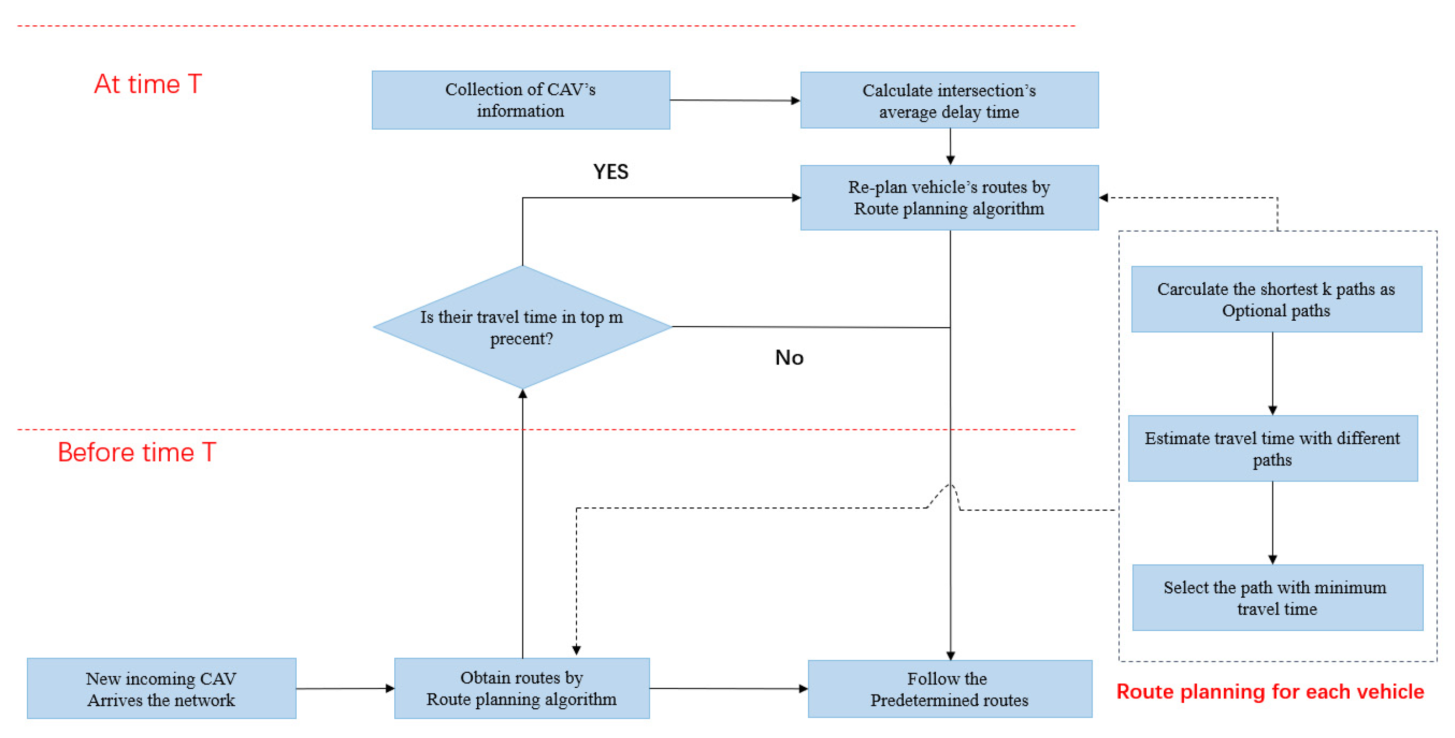
3.1. The Coordination Strategy in the MiRN

The time delay of a vehicle is related to the state of the intersection. As the arrival time of each vehicle is assigned by the RSU, we can estimate the delay for an approaching vehicle, i.e., vehicle $i$, by calculating the average delay of the vehicles in the intersection directly. $T_{j,t}^{*}$ represents the average delay of the CAVs in intersection $j$ at time $t$, and $C_{j,t}$ denotes the set of CAVs at the same time. Thus, we have:

$$T_{j,t}^{*}=\frac{1}{m}{\sum }_{i\in C_{j,t}}\left(t_{i,j}^{*}-t_{i,j}^{\min }\right).$$

(10)

Once the path of vehicle i is determined, the travel time for it to pass through the road network can be formulated as:

$$T_{i,h_{ik}}=T_{i,h_{ik}}^1+T_{i,h_{ik}}^2=\frac{dis\left(h_{ik}\right)}{v_c}+{\sum }_{j\in h_{ik}}{T}_{j,t}^{*}, h_{ik}\in L_i.$$

(11)

By calculating each intersection’s average delay time, we can estimate the travel time for the CAVs passing the selected path.

The CAVs in the MiRN are coordinated hierarchically, as shown in Figure 4. The RSU exchanges status and event information with the central controller in each cycle T, including the average delay time and the information on the new-coming CAVs. The central controller plans the path to minimize the travel time of the new-coming CAVs and sends it back to the corresponding RSU.

As the RSUs exchange information with the central controller periodically, the status information held by the central controller remains unchanged within one cycle, which results in an information updating delay. There is a chance that too many CAVs will be routed through the same intersections within the cycle, significantly changing the status of these intersections. A partial rerouting mechanism is employed to lessen the effect of the delay.

After the information exchange is conducted in cycle T, the central controller will choose a subset of CAVs to reroute their paths. The selection is based on the estimated travel time of each CAV; the longer the travel time, the greater the chance of being selected. Figure 5 shows the whole process.

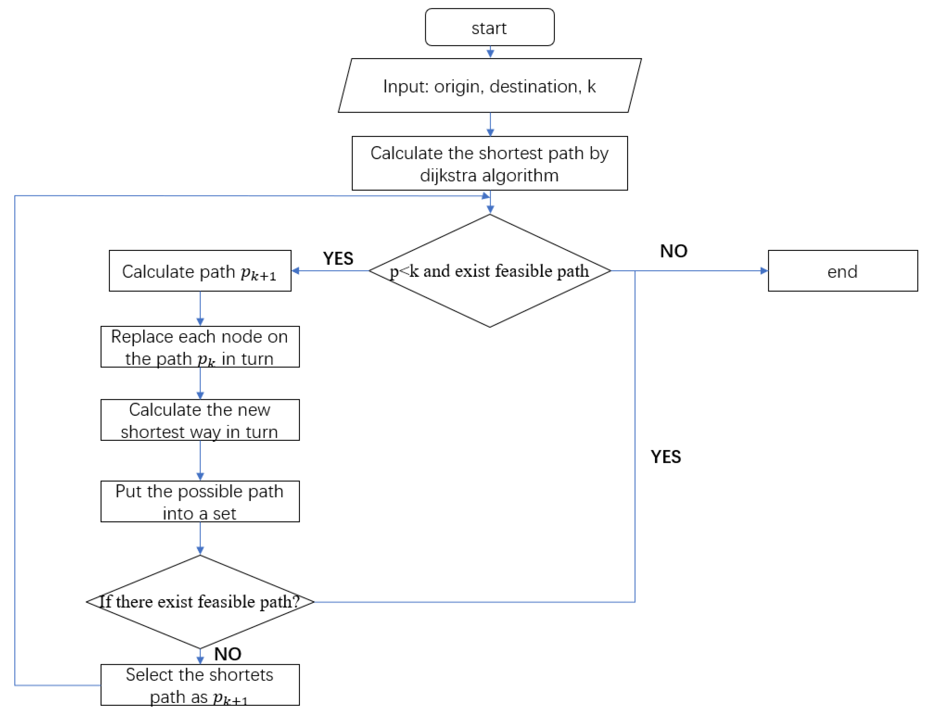
3.2. The Optimal Path Selection Algorithm

One possible method to find the optimal path is to enumerate all the shortest paths and calculate the corresponding travel times [33]. However, the shortest distance is not necessarily the shortest travel time. We introduce an adjustable parameter, k, as the number of candidate paths. We select the k-shortest paths as candidate paths through the greedy strategy.

The k-shortest paths problem in an undirected graph is a classical one in graph theory; it was first proposed by Hoffman and Pavley in 1959 [44] and was solved by Yen in 1971 [45]. We adopt Yen’s algorithm to find the k-shortest paths in the MiRN as optimal paths. Let $D_i$ stand for the candidate paths set and $P_i$ represent the k-shortest paths. Let $p_{mn}$ denote the n-th node on the m-th shortest path $h_{im}$. The process of finding the shortest k paths is shown in Figure 6.

The detailed steps are as follows: first, the shortest path for the CAVs can be calculated using the Dijkstra algorithm. Then, the other k − 1 shortest paths are determined recursively. When we obtain the shortest m paths, the (m + 1)-th shortest path can be calculated by the following four steps:

• Replace the node $p_{mn}$ with another feasible node $P_{mn}^{\prime }$ on the path $h_{im}$ and calculate the shortest path between $o_i$ and $p_{mn}^{\prime }$, $p_{mn}^{\prime }$ and $d_i$; then, we obtain an alternative path $h_{i\left(m+1\right)}^n$;
• Put $h_{i\left(m+1\right)}^n$ into the set $D_i$;
• Repeat 1 and 2 until all intersections are calculated;
• Calculate the lengths of the paths in the set $D_i$ and select the shortest one as the (m + 1)-th shortest path $h_{im+1}$. Remove $h_{im+1}$ from $D_i$ and put $h_{im+1}$ into $P_i$.

The algorithm terminates when the number of selected paths reaches k, or no more viable paths are available for the given origin and destination pair.

When the optimal paths are obtained, the travel time for CAVs with different paths can be estimated by Equations (11) and (12). Moreover, the path with minimum travel time is selected as the optimal path.

In summary, the optimal path selection Algorithm 1 is shown as follows:

Algorithm 1: A greedy algorithm to optimize the path for CAVs.

input: origin and destination of vehicle i; the number k of the alternative path

output: the optimal path 1: Calculate the shortest path with the Dijkstra algorithm 2: Put $h_{i1}$ into $P_i$ 3: while length($P_i$) < k and there exist feasible path do: 4:   for the last path $h_{im}^n$ in $P_i$ do: 5:     for each node $p_{mn}$ on the path $h_{im}^n$ do: 6:        replace the node $p_{mn}$ with $p_{mn}^{\prime }$ on the path $h_{im}^n$ 7:        calculate the shortest path between $o_i$ and $p_{mn}^{\prime }$, $p_{mn}^{\prime }$ and $d_i$ 8:       get the new alternative path $h_{i\left(m+1\right)}^n$ and put it in $D_i$ 9:     end for 10:   end for 11:   calculate the length of each path in $D_i$ 12:   put the shortest path $h_{im+1}$ into $P_i$ and remove it from $D_i$ 13: end while 14: estimate the travel time for the vehicle i using (11),(12) 15: select the path with minimal travel time as the optimal path

3.3. Scalability Discussion

To avoid searching all possible paths for each CAV, we prioritize the shorter paths over others through a greedy strategy. Then, we select the shortest $k$ paths as optimal paths. Moreover, as mentioned in Section 3.1, we use the average delay for each intersection to estimate the travel time for CAVs passing the intersection. In those two ways, we significantly reduced the computational complexity.

We also adjust the cycle time T to meet the computing and algorithm efficiency balance. The smaller the cycle time T is, the more often the intersection information is updated.

Furthermore, as traffic conditions change in real time, we reroute a certain percentage of CAVs with longer travel times to improve traffic efficiency. The higher the reroute rate, the lower the vehicle’s average delay time.

4. Simulation and Discussion

To validate the proposed algorithm, we implement our algorithm using Matlab R2016a on an Intel Core i7 CPU at 2.20 GHz with 16 GB RAM under a Windows 10 operating system. We use the intlinprog function in Matlab to solve the MILP problem (8) in isolated intersections. We reproduced the Yen’s algorithm for traffic scenarios and realized the coordination strategy in the MiRN through programming in MATLAB.

4.1. Simulation Settings

For simplicity and clarity, the simulation is carried out in a typical MiRN with six intersections, as shown in Figure 7. Two typical traffic flows are designed with a potential collision risk to verify the effectiveness of the path optimization algorithm proposed. We also compare our proposed method with the fixed signal time assignment method (STA) and the actuated STA [46] under the same settings, i.e., the road network and the traffic, as our proposed method. We reproduce the above two methods in the traffic simulation software SUMO v0.19.0 from Germany. Furthermore, the influence of varying parameters is also evaluated with different traffic, from sparse to crowded.

In our simulation, the lane’s width d is 3.5 m. Without loss of generality, for all vehicles, the length $\mathrm{l}=2.5\mathrm{m}$ and $\mathrm{w}=1.5\mathrm{m}$. The boundaries of the speed and acceleration are $v_{\max }=25\mathrm{m}$/s, $v_{\min }=5\mathrm{m}/\mathrm{s}$, $a_{\max }=5\mathrm{m}/{\mathrm{s}}^2$, and $a_{\min }=-5\mathrm{m}/{\mathrm{s}}^2$. The length of the CZ is ${\mathrm{L}}_1=90\mathrm{m}$. The length of the road segment between intersections is ${\mathrm{L}}_2=500\mathrm{m}$. The constant velocity of the CAVs traveling in the road segment is $v_c=15\mathrm{m}/\mathrm{s}$.

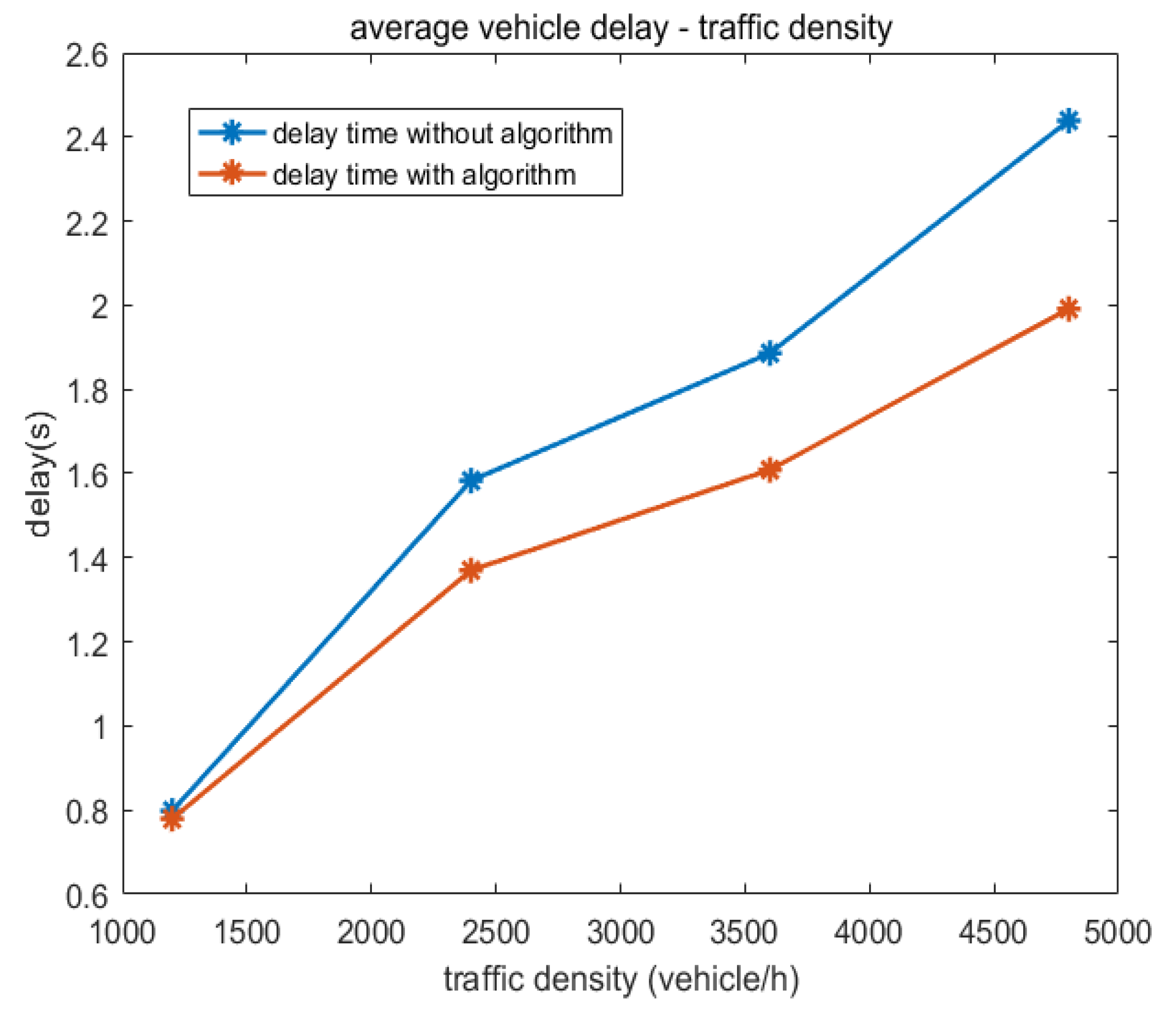
4.2. The Performance under Different Flow Rates

As is shown in Figure 8, we design two typical traffic flows with a potential collision risk in the simulation. We use the set of intersection numbers to represent the path of the CAVs. For traffic flow 1, there are three paths from the origin to the destination: $k_1^1=\left\{4,5,6,3\right\}$, $k_2^1=\left\{4,5,2,3\right\}$, $k_3^1=\left\{4,1,2,3\right\}$. The length of the three paths is the same. For traffic flow 2, there are also three paths from the origin to the destination: $k_1^2=\left\{6,5\right\}$, $k_2^2=\left\{6,3,2,5\right\}$, $k_3^2=\left\{6,3,2,1,4,5\right\}$. The length of the different paths varies greatly. Traffic flows 1 and 2 have potential collision risks at intersections 5 and 6. The simulation is carried out in four different flow rates, from sparse to crowded: $f_1=1200\mathrm{veh}/\mathrm{h}$, $f_2=2400\mathrm{veh}/\mathrm{h}$, $f_3=3600\mathrm{veh}/\mathrm{h}$, $f_4=4800\mathrm{veh}/\mathrm{h}$; we assume the cycle time $T=25\mathrm{s}$, the percent of replanning vehicles $\mathrm{m}=0.1,$ and the number of alternative paths $k=3$.

To evaluate the performance of our proposed optimal path selection algorithm, we compare it with the random path selection in the overall delays through the MiRN, as illustrated in Figure 8. In the compared strategy, the CAVs will select the shortest path as the optimal path, and when there are several shortest paths, the CAVs will randomly select one of them. According to Figure 9, our coordination algorithm can lower the average delay of the CAVs passing through the intersections in the MiRN. The greater the traffic density, the more effective our algorithm is. As an example, our strategy can reduce the overall delay by about 20% when the traffic density is $f_4=4800\mathrm{veh}/\mathrm{h}$.

Figure 10 compares the average intersection delay time using our algorithm against those without using our algorithm. It shows that the coordination strategy can effectively reduce the average delay in the intersection. With the traffic density $f_4=4800\mathrm{veh}/\mathrm{h}$, our algorithm lowered the average delays in intersections 5 and 6 by 15% and 28%, respectively.

4.3. Comparison among Three Coordination Strategies in MiRN

We compared our proposed method with the fixed and actuated STA methods frequently applied in the current transportation system. We reproduced the above two methods in SUMO, a free, open-source traffic simulation software. SUMO, it should be noted, does not support the controlling of the speed of each vehicle in detail. By editing the road network to be the same as that in the Matlab experiment, importing the vehicle occurrences and their origins and destinations exported from the Matlab experiment into SUMO, and setting up the traffic light strategies, we obtained the same settings as our proposed method to carry out the fixed STA method and actuated the STA experiments.

The cycle time of the fixed STA with four phases is set as 40 s. In the actuated STA, the minimum green time, maximum green time, and the maximum time gap between successive vehicles that will cause the current phase to be prolonged are 5 s, 45 s, and 5 s, respectively, and the yellow time is set as 3 s to ensure safety.

Table 2. Comparison results of different strategies in MiRN under different flow rates.

Flow Rate (veh/h)	Coordination Strategy	Average Travel Time (s)	Average Speed (m/s)
1200	The Proposed Method	52.963	24.413
	Fixed STA	325.750	3.991
	Actuated STA	203.565	6.39
2400	The Proposed Method	55.108	23.590
	Fixed STA	348.415	3.731
	Actuated STA	229.393	5.67
3600	The Proposed Method	57.813	22.486
	Fixed STA	355.723	3.655
	Actuated STA	232.048	5.602
4800	The Proposed Method	59.362	21.899
	Fixed STA	359.445	3.617
	Actuated STA	242.025	5.371

shows the three strategies’ average travel time and speed when passing through the road network.

The proposed strategy outperformed the other two STA-like methods greatly. Compared with the fixed STA, the proposed strategy reduced the average travel time by 83% under different flow rates. Compared with the actuated STA, the proposed approach reduced the average travel time by about 74% under different flow rates. The simulation results illustrate that the proposed method can improve the efficiency of CAVs in the MiRN.

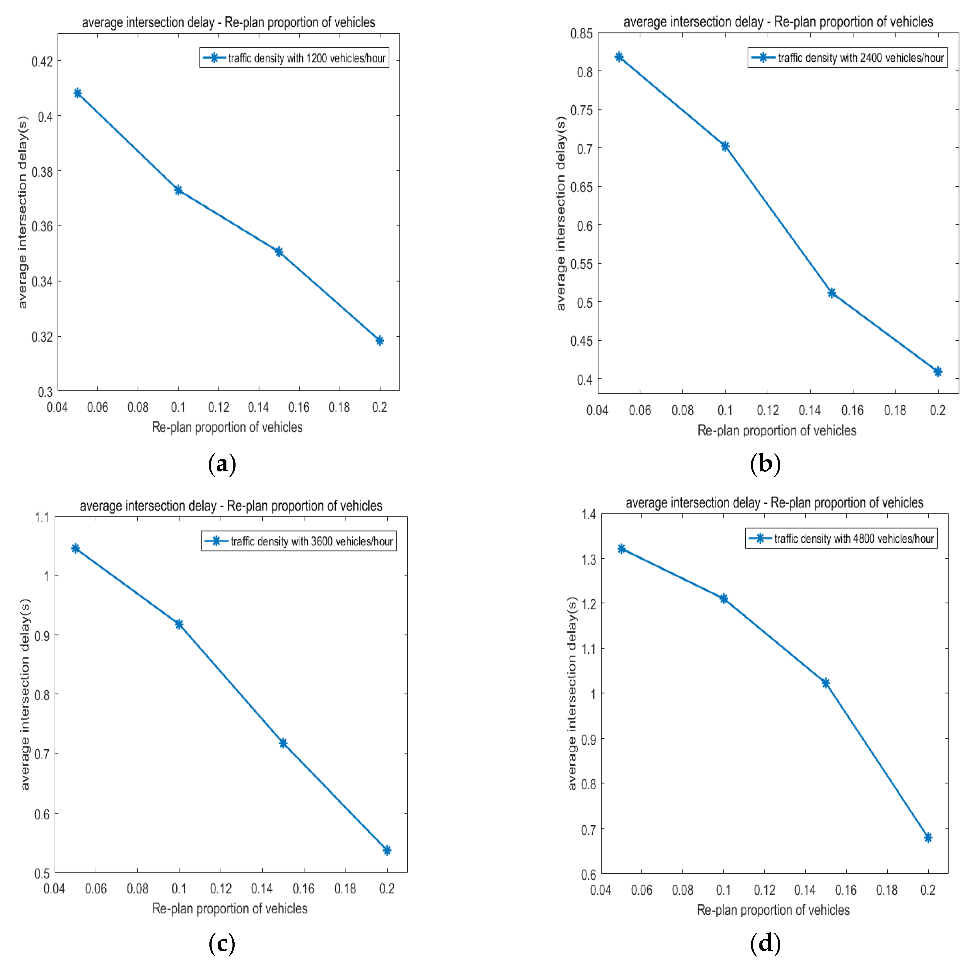
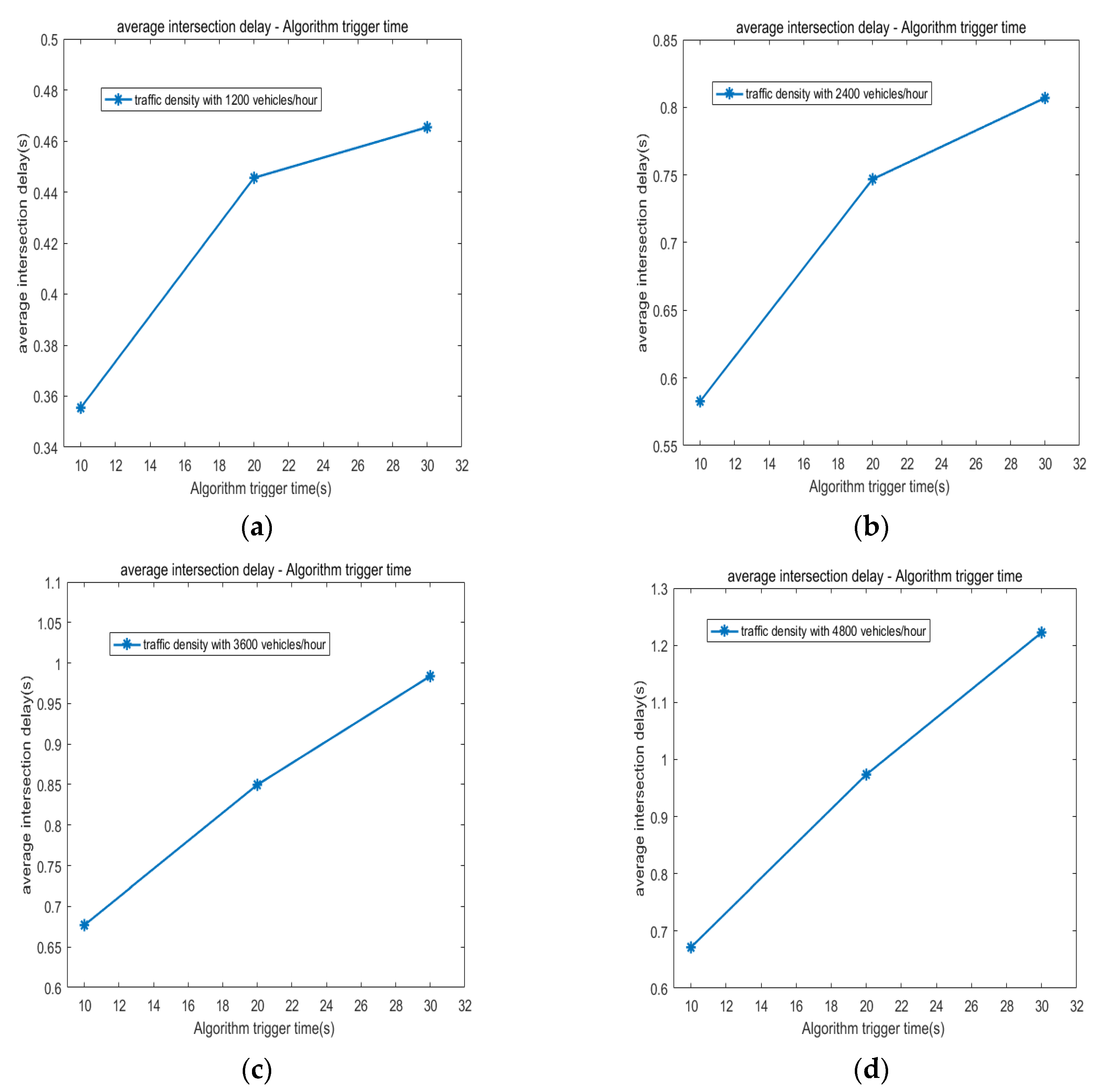
4.4. The Influence of Parameters under Different Flow Rates

The influence of the varying parameters on our algorithm performance is illustrated in Figure 11 and Figure 12.

With $T=25\mathrm{s}$ and k = 3, Figure 11 shows that the higher the proportion of vehicles rerouted, the lower the average delay time of the intersection is. The average delay time of the intersection with m set to be 0.2 is reduced by about 40–50%, compared with 0.05.

With $\mathrm{m}=0.1$ and $k=3$, Figure 12 shows that the smaller the cycle time T is, the lower the average delay time of the intersection is. The average delay time of the intersection with T set to be 10 s is reduced by 20–40% compared with the setting of $T=30\mathrm{s}$.

5. Conclusions

This paper proposes a novel vehicle coordination strategy in a multi-intersection road network. The suggested strategy includes an approach for efficiently estimating the travel time of CAVs and an optimal path selection algorithm that balances the computing and the effectiveness. The simulations demonstrate that the proposed strategy can approach sufficiently optimal solutions with different traffic densities. The impact of the parameters on our algorithm was also analyzed, both theoretically and experimentally.

Future work can extend the scenario to a more complex one, such as one with a mixed traffic environment consisting of CAVs and HDVs [47].

References

1. DESA, U. World Urbanization Prospects: The 2018 Revision Population Division; The United Nations: New York, NY, USA, 2019; pp. 1–104.
2. David, S.; Luke, A.; Bill, E.; Tim, L. 2021 Urban Mobility Report; Texas A&M Transportation Institute: College Station, TX, USA, 2021; (Online).
3. Batty, M.; Axhausen, K.W.; Giannotti, F.; Pozdnoukhov, A.; Bazzani, A.; Wachowicz, M.; Ouzounis, G.; Portugali, Y. Smart cities of the future. Eur. Phys. J. Spec. Top. 2012, 214, 481–518. [Google Scholar] [CrossRef] [Green Version]
4. Yang, K. Real-Time Urban Traffic Control in a Connected and Automated Vehicle Environment. Ph.D. Thesis, ETH Zurich, Zurich, Switzerland, 2018. [Google Scholar]
5. Xiong, Z.; Sheng, H.; Rong, W.; Cooper, D.E. Intelligent transportation systems for smart cities: A progress review. Sci. China Inf. Sci. 2012, 55, 2908–2914. [Google Scholar] [CrossRef] [Green Version]
6. Law, K.H.; Lynch, J.P. Smart City: Technologies and Challenges. IT Prof. 2019, 21, 46–51. [Google Scholar] [CrossRef]
7. Menouar, H.; Guvenc, I.; Akkaya, K.; Uluagac, A.S.; Kadri, A.; Tuncer, A. UAV-Enabled Intelligent Transportation Systems for the Smart City: Applications and Challenges. IEEE Commun. Mag. 2017, 55, 22–28. [Google Scholar] [CrossRef]
8. Ahmed, H.U.; Huang, Y.; Lu, P.; Bridgelall, R. Technology Developments and Impacts of Connected and Autonomous Vehicles: An Overview. Smart Cities 2022, 5, 382–404. [Google Scholar] [CrossRef]
9. Huang, Y.; Wang, H.; Khajepour, A.; Ding, H.; Yuan, K.; Qin, Y. A novel local motion planning framework for autonomous vehicles based on resistance network and model predictive control. IEEE Trans. Veh. Technol. 2020, 69, 55–66. [Google Scholar] [CrossRef]
10. Singh, S. Critical reasons for crashes investigated in the national motor vehicle crash causation survey. (No. DOT HS 812 115); In Traffic Facts–Crash Stats; US Department of Transportation: Washington, DC, USA, 2015. [Google Scholar]
11. Rios-Torres, J.; Malikopoulos, A.A. A Survey on the Coordination of Connected and Automated Vehicles at Intersections and Merging at Highway On-Ramps. IEEE Trans. Intell. Transp. Syst. 2017, 18, 1066–1077. [Google Scholar] [CrossRef]
12. Agarwal, V.; Sharma, S.; Agarwal, P. IoT Based Smart Transport Management and Vehicle-to-Vehicle Communication System. In Computer Networks, Big Data and IoT; Springer: Singapore, 2021; pp. 709–716. [Google Scholar]
13. Ezenwa, L. Wireless V2V Communication with DSRC Technology in Comparison to C-V2X. ATZ Worldw 2022, 124, 40–43. [Google Scholar] [CrossRef]
14. Shah, K.; Chadotra, S.; Tanwar, S.; Gupta, R.; Kumar, N. Blockchain for IoV in 6G environment: Review solutions and challenges. Clust. Comput. 2022, 25, 1927–1955. [Google Scholar] [CrossRef]
15. National Highway Traffic Safety Administration. Automated Driving Systems 2.0: A Vision for Safety; US Department of Transportation, DOT HS: Washington, DC, USA, 2017; Volume 812, p. 442.
16. Bergen, M. Alphabet Launches the First Taxi Service with No Human Drivers. Retrieved from Bloomberg Technology. 2017. Available online: https://bloom.bg/2Ea2dml (accessed on 22 April 2022).
17. Lee, T.B. Fully Driverless Cars Could be Months Away. Ars Tech. 2017, 3. (Online). [Google Scholar]
18. Dong, C.; Chen, X.; Dong, H.; Yang, K.; Guo, J.; Bai, Y. Research on Intelligent Vehicle Infrastructure Cooperative System Based on Zigbee. In Proceedings of the 2019 5th International Conference on Transportation Information and Safety (ICTIS), Liverpool, UK, 14–17 July 2019; pp. 1337–1343. [Google Scholar]
19. Gao, J.; Cao, C.; Li, W.; Li, X. Research and Verification of Risk Prevention Methods for Commercial Vehicles Based on Intelligent Vehicle and Infrastructure System. In Proceedings of the 2020 4th Annual International Conference on Data Science and Business Analytics (ICDSBA), Changsha, China, 5–6 September 2020; pp. 191–194. [Google Scholar]
20. Chu, W.; Wuniri, Q.; Du, X.; Xiong, Q.; Huang, T.; Li, K. Cloud Control System Architectures, Technologies and Applications on Intelligent and Connected Vehicles: A Review. Chin. J. Mech. Eng. 2021, 34, 139. [Google Scholar] [CrossRef]
21. Molina, C.B.S.T.; Almeida, J.R.d.; Vismari, L.F.; González, R.I.R.; Naufal, J.K.; Camargo, J. Assuring Fully Autonomous Vehicles Safety by Design: The Autonomous Vehicle Control (AVC) Module Strategy. In Proceedings of the 2017 47th Annual IEEE/IFIP International Conference on Dependable Systems and Networks Workshops (DSN-W), Denver, CO, USA, 26–29 June 2017; pp. 16–21. [Google Scholar]
22. Subraveti, H.H.S.N.; Srivastava, A.; Ahn, S.; Knoop, V.L.; van Arem, B. On lane assignment of connected automated vehicles: Strategies to improve traffic flow at diverge and weave bottlenecks. Transp. Res. Part C: Emerg. Technol. 2021, 127, 103126. [Google Scholar] [CrossRef]
23. Tachet, R.; Santi, P.; Sobolevsky, S.; Reyes-Castro, L.I.; Frazzoli, E.; Helbing, D.; Ratti, C. Revisiting Street Intersections Using Slot-Based Systems. PLoS ONE 2016, 11, e0149607. [Google Scholar] [CrossRef] [PubMed] [Green Version]
24. Mahbub, A.; Karri, V.; Parikh, D.; Jade, S.; Malikopoulos, A.A. A Decentralized Time- and Energy-Optimal Control Framework for Connected Automated Vehicles: From Simulation to Field Test. arXiv 2019, arXiv:1911.01380. [Google Scholar]
25. Jiang, Z.; Yu, D.; Zhou, H.; Luan, S.; Xing, X. A Trajectory Optimization Strategy for Connected and Automated Vehicles at Junction of Freeway and Urban Road. Sustainability 2021, 13, 9933. [Google Scholar] [CrossRef]
26. Chai, L.; Shen, G.; Ye, W. The Traffic Flow Model for Single Intersection and Its Traffic Light Intelligent Control Strategy. In Proceedings of the 2006 6th World Congress on Intelligent Control and Automation, Dalian, China, 21–23 June 2006; pp. 8558–8562. [Google Scholar]
27. Garg, V.; Sachan, A.; Kumar, N.; Mittal, S. Congestion Control Utilizing Software Defined Control Architecture at the Traffic Light Intersection. In Proceedings of the 2021 IEEE 18th International Conference on Mobile Ad Hoc and Smart Systems (MASS), Denver, CO, USA, 4–7 October 2021; pp. 597–602. [Google Scholar]
28. Meng, Y.; Li, L.; Wang, F.; Li, K.; Li, Z. Analysis of cooperative driving strategies for Nonsignalized intersections. IEEE Trans. Veh. Technol. 2018, 67, 2900–2911. [Google Scholar] [CrossRef]
29. Huang, S.; Sadek, A.W.; Zhao, Y. Assessing the mobility and environmental benefits of reservation-based intelligent intersections using an integrated simulator. IEEE Trans. Intell. Transp. Syst. 2012, 13, 1201–1214. [Google Scholar] [CrossRef]
30. Zhang, Y.; Malikopoulos, A.A.; Cassandras, C.G. Decentralized optimal Control for connected automated vehicles at intersections including left and right turns. In Proceedings of the 2017 IEEE 56th Annual Conference on Decision and Control (CDC), Melbourne, VIC, Australia, 12–15 December 2017; pp. 4428–4433. [Google Scholar]
31. Rahmati, Y.; Talebpour, A. Towards a collaborative connected, automated driving environment: A game theory based decision framework for unprotected left turn maneuvers. In Proceedings of the IEEE Intelligent Vehicles Symposium (IV), Los Angeles, CA, USA, 11–14 June 2017. [Google Scholar]
32. Dong, H.; Dai, Z. A multi intersections signal coordinate control method based on game theory. In Proceedings of the 2011 International Conference on Electronics, Communications and Control (ICECC), Ningbo, China, 9–11 September 2011; pp. 1232–1235. [Google Scholar]
33. Miculescu, D.; Karaman, S. Polling-Systems-Based Autonomous Vehicle Coordination in Traffic Intersections With No Traffic Signals. IEEE Trans. Autom. Control. 2020, 65, 680–694. [Google Scholar] [CrossRef]
34. Ahn, H.; del Vecchio, D. Safety Verification and Control for Collision Avoidance at Road Intersections. IEEE Trans. Autom. Control. 2018, 63, 630–642. [Google Scholar] [CrossRef]
35. Li, L.; Wang, F. Cooperative driving at adjacent blind intersections. In Proceedings of the 2005 IEEE International Conference on Systems, Man and Cybernetics, Waikoloa, HI, USA, 12 October 2005. [Google Scholar]
36. Ashtiani, F.; Fayazi, S.A.; Vahidi, A. Multi-intersection traffic management for autonomous vehicles via distributed mixed-integer linear programming. In Proceedings of the 2018 Annual American Control Conference (ACC), Milwaukee, WI, USA, 27–29 June 2018; pp. 6341–6346. [Google Scholar]
37. Chalaki, B.; Malikopoulos, A.A. An optimal coordination framework for connected and automated vehicles in two interconnected intersections. In Proceedings of the 2019 IEEE Conference on Control Technology and Applications (CCTA), Hong Kong, China, 19–21 August 2019; pp. 888–893. [Google Scholar]
38. Darmoul, A.S.; Elkosantini, S.; Louati, A.; Said, L.B. Multi-agent immune networks to control interrupted flow at signalized intersections-ScienceDirect. Transp. Res. Part C: Emerg. Technol. 2017, 82, 290–313. [Google Scholar] [CrossRef]
39. Chin, Y.K.; Kow, W.Y.; Khong, W.L.; Tan, M.K.; Teo, K.T.K. Q-Learning Traffic Signal Optimization within Multiple Intersections Traffic Network. In Proceedings of the 2012 Sixth UKSim/AMSS European Symposium on Computer Modeling and Simulation, Malta, Malta, 14–16 November 2012; pp. 343–348. [Google Scholar]
40. Pei, H.; Zhang, Y.; Tao, Q.; Feng, S.; Li, L. Distributed Cooperative Driving in Multi-Intersection Road Networks. IEEE Trans. Veh. Technol. 2021, 70, 99. [Google Scholar] [CrossRef]
41. Wang, Y.; Cai, P.; Lu, G. Cooperative autonomous traffic organization method for connected automated vehicles in multi-intersection road networks. Transp. Res. Part C Emerg. Technol. 2020, 111, 458–476. [Google Scholar] [CrossRef]
42. Li, L.; Wang, F. Cooperative driving at blind crossings using intervehicle communication. IEEE Trans. Veh. Technol. 2006, 55, 1712–1724. [Google Scholar] [CrossRef]
43. Boukouvala, F.; Misener, R.; Floudas, C.A. Global optimization advances in Mixed-Integer Nonlinear Programming, MINLP, and Constrained Derivative-Free Optimization, CDFO. Eur. J. Oper. Res. 2016, 252, 701–727. [Google Scholar] [CrossRef] [Green Version]
44. Hoffman, W.; Pavley, R. A method of solution of the Nth best path problem. J. ACM 1959, 6, 506–514. [Google Scholar] [CrossRef]
45. Yen, J.Y. Finding the k shortest loopless paths in a network. Manag. Sci. 1971, 17, 712–716. [Google Scholar] [CrossRef]
46. Chen, L.; Hu, T. Flow Equilibrium Under Dynamic Traffic Assignment and Signal Control—An Illustration of Pretimed and Actuated Signal Control Policies. IEEE Trans. Intell. Transp. Syst. 2012, 13, 1266–1276. [Google Scholar] [CrossRef]
47. Mahbub, A.M.I.; Le, V.-A.; Malikopoulos, A.A. Safety-Aware and Data-Driven Predictive Control for Connected Automated Vehicles at a Mixed Traffic Signalized Intersection. arXiv 2022, arXiv:2203.05739. [Google Scholar]
Figure 1. A typical road network with four intersections.
Energies 15 05168 g001
Figure 2. The weighted undirected graph describes the road network. Numbers 1–6 indicate the intersection number.
Energies 15 05168 g002
Figure 3. Illustration of two kinds of collisions in the isolated intersection.
Energies 15 05168 g003
Figure 4. Illustration of exchanging information between RSUs and the central controller at an isolated intersection. Numbers 1–4 represent the intersection number.
Energies 15 05168 g004
Figure 5. The process of the coordination strategy.
Energies 15 05168 g005
Figure 6. Flowchart to find the k-shortest paths in MiRN.
Energies 15 05168 g006
Figure 7. A typical road network with six intersections. Numbers 1–6 stand for the intersection number.
Energies 15 05168 g007
Figure 8. Illustration of two typical traffic flows in a road network. Numbers 1–6 indicate the intersection number.
Energies 15 05168 g008
Figure 9. Comparison of vehicle’s delay with coordination strategy and without coordination strategy in different traffic densities.
Energies 15 05168 g009
Figure 10. Comparison of delay with coordination strategy and without coordination strategy in different traffic densities: (a) intersection 5 and (b) intersection 6.
Energies 15 05168 g010
Figure 11. The relation between the parameter m and the average intersection delay with different traffic densities: (a) f 1 = 1200   veh / h , (b) f 2 = 2400   veh / h , (c) f 3 = 2400   veh / h , (d) f 4 = 4800   veh / h .
Energies 15 05168 g011
Figure 12. The relation between the parameter T and the average intersection delay with different traffic densities: (a) f 1 = 1200   veh / h , (b) f 2 = 2400   veh / h , (c) f 3 = 2400   veh / h , (d) f 4 = 4800   veh / h .
Energies 15 05168 g012