
The Dynamic Spillover between Renewable Energy, Crude Oil and Carbon Market: New Evidence from Time and Frequency Domains

1
School of Economics and Management, North China Electric Power University, Beijing 102206, China
2
School of Environment, Education & Development, The University of Manchester, Manchester M13 9PL, UK
*
Author to whom correspondence should be addressed.
Energies 2022, 15(11), 3927; https://doi.org/10.3390/en15113927
Submission received: 21 April 2022
/
Revised: 17 May 2022
/
Accepted: 18 May 2022
/
Published: 26 May 2022
(This article belongs to the Special Issue Behavioral Models for Energy with Applications)
Abstract
:To obtain the price return and price volatility spillovers between renewable energy stocks, technology stocks, oil futures and carbon allowances under different investment horizons, this paper employs a frequency-dependent method to study the dynamic connectedness between these assets in four frequency bands. The results show that, first, there is a strong spillover effect between these assets from a system-wide perspective, and it’s mainly driven by short-term spillovers. Second, in the time domain, technology stocks have a more significant impact on renewable energy stocks compared to crude oil. However, through the study in the frequency domain, we find renewable energy stocks exhibit a more complex relationship with the other two assets at different time scales. Third, renewable energy stocks have significant spillover effect on carbon prices only in the short term. On longer time scales, other factors such as energy prices, climate and policy may have a greater impact on carbon allowance prices. Fourth, the spillover effect of the system is time-varying and frequency-varying. During the European debt crisis, the international oil price decline and the COVID-19 pandemic, the total spillover index of the system has experienced a substantial increase, mainly driven by medium, medium to long or long term spillovers.
1. Introduction
Growing concerns about energy security, climate change, and energy shortage have aroused people’s awareness of increasing the proportion of low-carbon energy in total energy consumption, and the renewable energy sector has become one of the fastest-growing energy sectors. As of the end of 2018, the estimated share of renewable energy power generation in the total global power generation exceeded 26%, and renewable energy accounted for more than one-third of the global installed power generation capacity [1]. The renewable energy sector has attracted remarkable investment, with more than $280 billion invested in renewable power and fuels each year during 2015–2018, and with more renewable energy net capacity additions than fossil and nuclear energy combined [1]. In addition, renewable energy sources will play an increasingly important role in meeting the world’s growing energy needs [2]. According to the International Energy Agency’s (IEA) 2019 World Energy Outlook, under the Stated Policies Scenario, more than half of the increase in global energy demand by 2040 will be met by low-carbon energy sources [3].
The rapid development and promising prospects of the renewable energy industry have stimulated the interest of private investors in renewable energy stocks. Research on the relationship between renewable energy stocks and other assets has grown in recent years, focusing on issues such as interdependence, causality, or spillover effect between renewable energy stocks, crude oil, or technology stocks. First, as crude oil plays an important role in global energy supply and substitutes with renewable energy, many studies have been conducted on the relationship between crude oil and renewable energy stocks. Henriques and Sadorsky, Kumar et al. and Ahmad et al., stated that rising oil prices have a positive impact on renewable energy stock prices [4,5,6]. Reboredo and Ugolini and Song et al., studied the relationship between various fossil energies and renewable energy stocks, and found that crude oil price is the main factor affecting the price fluctuation of renewable energy [7,8]. Pham further analyzed the relationship between the stock performance of clean energy subsectors and the prices of crude oil, and they came to conclusion that the correlation between different sub-sectors and the price of crude oil varies. It is worth noting that some scholars have found that the correlations between crude oil prices and renewable energy stock prices or technology stocks have different features in different time periods or time scales. Managi and Okimoto introduced Markov-switching framework and found that there is a structural break in the system composed of crude oil, clean energy stocks and technology stocks at the end of 2007. Before the structural break, crude oil price had no significant impact on clean energy stocks, but the oil price shock after the structural change has a significant positive impact on renewable energy stocks [9]. By employing Detrended Cross-Correlation Analysis (DCCA) framework, Paiva et al. found that crude oil and renewable energy are highly correlated only from mid-2008 to mid-2012 [10]. Reboredo et al. used wavelet method to find that the interactions between crude oil prices and renewable energy stock prices are weak in the short term, and there is no linear Granger causality, but the dependence between the two increases in the longer time scale [11].
Second, some scholars use different econometric methods and find that compared with the price of crude oil, there is a stronger correlation or spillover effect between technology stocks prices and renewable energy stock prices. Henriques and Sadorsky built a four-variable VAR model and found that the volatility of technology stocks has a greater impact on renewable energy stocks than that of crude oil prices [4]. By constructing a multivariate GARCH model, Sadorsky found that the dynamic correlation between clean energy stocks and technology stocks is higher than that between clean energy and oil prices [12]. Ahmad took more asset types into account based on Sadorsky’s research and came to a similar conclusion [13]. Inchauspe et al., constructed an asset pricing model with time-varying parameters and found that the price returns of renewable energy stocks are much less affected by oil prices than those of technology stocks [14]. Zhang and Du established a TVP-SV-VAR model to study the dynamic relationship between the stock prices of renewable energy, high-tech and fossil fuel companies, and found that renewable energy companies stock prices have a stronger correlation with high-tech stocks [15]. Tiwari et al., investigated the tail dependence between crude oil, clean energy and technology stocks in different market scenarios and discovered that oil price volatility is not a key factor affecting the profitability of clean energy and technology companies, while clean energy and technology companies are strongly correlated [16]. In addition, some scholars further find that there are differences in the correlations between crude oil, renewable energy stocks and technology stocks at different time scales. Ferrer et al., believed that the correlation between crude oil prices and renewable energy stock prices is low in both the short and long term, while there is a significant volatility spillover effect between technology stock prices and renewable energy stock prices in the short term [17]. Through threshold cointegration test, Bondia et al., found that in the short run, alternative energy stocks are affected by technology stocks, oil prices, and interest rates; in the long run, alternative energy stocks are not affected by these factors [18]. By constructing a cointegrating nonlinear auto-regressive distributed lag (NARDL) model, Kocaarslan and Soytas found that a rise in oil prices in the short term leads to an increase in clean energy investment, but in the long run, the price of crude oil has a negative impact on clean energy; in both the short and long term, there is a significant two-way positive effect between technology stocks and clean energy stocks [19].
Third, carbon pricing policies aimed at mitigating climate change can also stimulate interest in renewable energy, but only a small number of studies have taken the carbon allowances price into account when exploring the volatility of renewable energy stock prices. Dutta et al., found that, by building the VAR-GARCH model, in Europe, the correlation between carbon allowances and the price return of clean energy stocks is not significant, but there is a significant volatility correlation between them [20]. Xia et al., stated that electricity, coal or oil prices contribute more to changes in renewable energy earnings than carbon allowance prices [21]. Lin and Chen, Jiang et al., took China’s carbon emission trading (CET) market as an example to study the correlation between carbon prices and renewable energy stock prices. Lin and Chen found that there is no significant volatility spillover effect between China’s carbon market and renewable energy stocks market, while Jiang et al., believed that renewable energy stocks have an impact on carbon allowance prices in the short and middle term [22,23].
Despite the growing body of research on the relationship between renewable energy stocks and assets such as crude oil, technology stocks or carbon allowances, there are still some research gaps. One of them is that few scholars pay attention to the interaction between renewable energy stocks and other assets in different frequency domains. However, given that different institutions differ in how they respond to and pay attention to information over different time horizons, we believe it is important to understand the frequency dynamics between renewable energy stocks and other assets. For market investors, due to different goals, preferences and risk tolerance, they often have different investment horizons. Specifically, short-term investors, such as day traders or hedge funds, will pay more attention to the short-term performance of the market, while long-term investors, such as large investment institutions, will more focus on the long-term performance of the market and adjust their investment strategies. Another research gap is that there are few studies on the relationship between carbon allowance prices and renewable energy stock prices. However, as the importance of global carbon emission reduction becomes increasingly prominent, it is of theoretical and practical significance to study the relationship between carbon allowance and renewable energy stocks. This paper introduces a recently developed connectedness approach to study the price return and price volatility among renewable energy stocks, global stock index, technology stocks, crude oil futures, carbon allowances, and the 10-year US Treasury note both in time domain and frequency domain.
The contributions of this research are mainly lie in the following four points:
First, this paper may be the first study to examine the spillover effect between renewable energy stocks, crude oil, technology stocks, and carbon allowances from a systematic perspective. To our knowledge, there are no studies on renewable energy spillovers that consider both technology stocks and carbon allowances. We believe it’s necessary to consider both assets because: (i) some studies show a stronger correlation or spillover effect between technology stocks and renewable energy stocks compared to crude oil; (ii) carbon pricing policies can stimulate interest in renewable energy, and some studies have shown that there is a positive correlation between carbon allowances and clean energy stocks.
Second, this paper uses a newly developed network connectedness approach to study the dynamic spillovers among renewable energy stocks and other assets over different investment horizons. Investors tend to choose different horizons due to their different objectives, preferences, and risk tolerance, yet there is a lack of research on the frequency dynamics between renewable energy stocks and other assets. The connectedness method proposed by Barunik and Krehlik, which adds the investigation on the frequency dynamics of connectedness on the basis of the connectedness network method proposed by Diebold and Yilmaz, and has been gradually applied to the fields of energy and finance in recent years [17,24,25,26]. Many existing studies on the relationship between renewable energy stocks and other assets use VAR and GARCH models and investigate the relationship between variables in the time domain through these types of econometric models, while this paper investigates the interactions between renewable energy stocks and other assets in both time and frequency domains.
Third, this paper studies both price return and price volatility spillovers, and research on these two channels can help investors and policy makers better understand the interactions between markets. In theory, renewable energy stocks can be linked to other financial markets, energy markets or carbon allowance markets through two ways. One is price return spillovers that occur during price discovery process, during which a price change in one market has an impact on the value of an asset in other markets, resulting in changes in their prices [27,28,29]. The other is price volatility spillovers, in which the willingness of market participants to hold assets in other markets may change when one market fluctuates. To our knowledge, the spillovers of these assets under both channels have not been studied.
Fourth, this paper covers the period from the 2008 financial crisis to the 2021 COVID-19 pandemic, and separately studies the dynamic spillovers between renewable energy stocks and other assets during European debt crisis, oil price drop, and COVID-19 pandemic.
This paper can provide some implications to policy makers and investors for market or asset management, which will be conducive to maintain the stability of energy market or financial market, promote the development of renewable energy industry, and improve the risk management strategies of market investors. For policy makers, first, by studying the connectedness between the volatility of the renewable energy sector and the crude oil market at different scales, it is possible to assess the risk spillovers between markets and improve the price mechanism to prevent the market from violent turmoil. Second, by investigating the strength of the spillover effect between the returns of the renewable energy sector and crude oil and technology industries, it helps policy makers to evaluate the impact of other industries on the asset value of the renewable energy industry and to formulate corresponding policies to promote the development of the renewable energy industry. Third, studying the dynamic spillover effect between carbon allowances prices and the renewable energy sector is conducive to measuring the impact of carbon trading on the renewable energy sector in a quantitative and dynamic manner, and helps to assess the role of emission trading scheme in promoting the development of renewable energy. For market investors, the study of returns and volatility spillovers between various assets such as renewable energy stocks, crude oil, technology stocks and carbon allowances over different investment horizons will help investors to adjust the asset allocation of their portfolios in a timely manner. Investors can effectively reduce the market risk of investment by selecting assets with a certain hedging effect in an investment portfolio. In addition, portfolio management by investors is more difficult in times of turmoil in financial or energy markets. This paper analyzes the interactions between a large set of assets during the European debt crisis, the international oil price decline and the COVID-19 pandemic, which can provide a reference for investors in developing an asset diversification strategy. The remainder of the paper is organized as follows: The Section 2 introduces the connectedness network approach proposed by Barunik and Krehlik; The Section 3 describes the variables and makes a preliminary analysis of the data; In the Section 4, we represent the empirical results of the connectedness analysis in time and frequency domain; The Section 5 summarizes the main findings and makes implications for market investors and policy makers.
2. Empirical Methodology
This study applies the frequency-dependent connectedness methodology given by Barunik and Krehlik to estimate the spillovers among renewable energy stock prices, technology stock price, world stock market price, oil price, carbon price, and bond price [26]. By extending the connectedness approach proposed by Diebold and Yilmaz in 2014, this technique can measure the connectedness both in the time and frequency domains [25].
2.1. Measuring Connectedness in the Time Domain
The connectedness network approach recently proposed by Diebold and Yilmaz in 2014 is based on a VAR model approach and has been widely used to measure the linkages between financial or energy markets in time domain [30,31,32,33,34,35,36]. Within the vector autoregressive (VAR) framework, all variables are assumed to be endogenous, and the dynamics of each variable are affected by the lags of all variables and an error term. In our analysis, we assume the price series are modeled as a VAR model of order p,
where is an vector of endogenous variables, and is an vector of independently distributed errors. is an matrix of regression coefficients to be estimated and with is an identity matrix. Given the assumption of stationarity of the VAR model, Equation (1) can be converted into an infinite order vector moving average (VMA) representation as,
where matrix lag-polynomial can be calculated recursively from . Based on the generalized variance decomposition framework proposed by Koop et al., and Pesaran and Shin, Diebold and Yilmaz define the contribution of the jth variable to the variance of forecast error of the element i at horizon h as [37,38],
where , is the forecast horizon and is an matrix of moving average coefficients at lag . Thus, a connectedness matrix can be constructed with elements. The contributions of in the matrix can be normalized as,
and and .
The total spillover in the whole system can be measured as,
To determine how much one variable contributes to the system and how much information it gains from the system, the total directional connectedness is computed as,
Furthermore, the net directional connectedness can be constructed as,
If , it means variable i contributes more than it gains from the system and variable i is a net information transmitter of the system, otherwise, variable i is a net information receiver of the system.
Similarly, the net pairwise connectedness between variable i and variable j can be written as,
If , it means variable i contributes more than it gains from variable j and variable i is a net information transmitter to j, otherwise, variable i is a net information receiver from j.
2.2. Measuring Connectedness in the Frequency Domain
Barunik and Krehlik extend the connectedness network model proposed by Diebold and Yilmaz by adopting spectral methods to investigate the spillover effect in the frequency domain.
Consider a frequency response function , , which can be obtained as a Fourier transform of the coefficients , with . The spectral density of at frequency can then be described as,
The power spectrum is a key quantity for understanding frequency dynamics since it describes how the variance of the is distributed over the frequency components . Then, the generalized causation spectrum over frequencies is defined as,
where measures how much the spectrum of the ith variable at a given frequency due to shocks in the jth variable. To study economic problems in different time horizons, it is more convenient to work with frequency bands that we define as the amount of forecast error variance created on a convex set of frequencies. Given an arbitrary frequency band , , , the generalized variance decompositions on frequency band d are defined as,
where . Suppose is wide-sense stationary with , . Then,
The scaled generalized variance decomposition on the frequency band is defined as,
Denote by an interval on the real line from the set of intervals that from a partition of the interval , such that , and , we have . Based on the spillover measures proposed by Diebold and Yilmaz in 2014, the overall spillover on frequency band can be computed as,
where is the trace operator, and denotes the sum of all elements of the matrix. only gives us the spillovers that occurs within the frequency band, and we refer to as “within spillover”. To measure the contribution of a given frequency band to the aggregate measure, the “frequency spillover” is defined as,
The “frequency spillover” decomposes the overall connectedness defined in Equation (5) into distinct parts such that . Similarly, we can define for each variable i a measure of variance contributed by variable j as,
The directional connectedness on the spectral band can be constructed as,
and the net directional connectedness and net pairwise connectedness can be computed as,
3. Data
This paper uses daily prices of renewable energy stocks, high-technology stocks, global stock index, crude oil futures, EUA carbon futures and 10-year US Treasury note. Except for the global stock index, which is obtained from the DataStream database, all other data are obtained from the Bloomberg database. The total sample period is from 25 June 2008 to 9 June 2021, containing a total of 3261 observations.
3.1. Data Description
This paper selects The Wilder Hill New Energy Global Innovation Index (NEX) for renewable energy stock prices. NEX is an equal-dollar-weighted index to track important companies whose innovative technologies and services focus on generation and use of cleaner energy, decarbonization, and efficiency. The NEX is the first and leading global index for clean, alternative, and renewable energy. As of the second quarter of 2021, NEX covers 125 stocks from a variety of countries in the Americas, Europe, Asia, and other regions. These companies operate in a variety of renewable energy sectors with the following weights: Energy Conversion (16%), Energy Efficiency (13%), Energy Storage (16%), Biofuels and Biomass (9%), Solar Energy (4%), Wind Energy (24%), and Others (18%) [39]. NEX is widely used in research on renewable energy stocks performance [5,14,18]. We believe that NEX is a good proxy for the financial performance of global renewable energy companies due to its extensive coverage area and diversified sectors.
Some existing studies have found that the technology company stock is an important factor influencing the stocks of renewable energy companies [4,5,9,12]. This paper considers that the stock prices of technology companies is a factor that cannot be ignored in the research of renewable energy companies. For the stock prices of technology companies, we select The NYSE Arca Tech 100 Index (PSE). The NYSE Arca Tech 100 Index is designed to provide a benchmark for measuring the performance of technology-related companies operating across a broad spectrum of industries. The index is a price-weighted index comprised of common stocks and American Depository Receipts (ADRs) of technology-related companies listed on US exchanges. Companies from different industries that produce or deploy innovative technologies to conduct their business are considered for inclusion. Leading companies are selected from several industries, including computer hardware, software, semiconductors, telecommunications, data storage and processing, electronics, media, aerospace and defense, health care equipment, and biotechnology [40].
As for carbon price, this paper selects the future prices of European Union Allowances (EUAs) of European Union (EU) Emission Trading Scheme (ETS). ETS is a cap-and-trade scheme first introduced in EU to promote carbon emission mitigation and the development of renewable energy technology, and has received attention in recent years on the research of renewable energy stock prices [5,6,21].
For global stock price index, this paper selects the MSCI World index. The MSCI World index is a broad global equity benchmark designed to represent performance of the full opportunity set of stocks. As of July 2021, It covers more than 1559 securities across large and mid-cap size segments and across style and sector segments in 23 developed [41]. As of 30 June 2020, the MSCI World index includes countries and their respective weights as follows, the US (65.53%), Japan (7.96%), the UK (4.41%), France (3.41%), Switzerland (3.32%), Canada (3.13%), Germany (2.90%), Australia (2.11%), Netherlands (1.35%) and Others (Austria, Belgium, Denmark, Finland, Hong Kong, Ireland, Israel, Italy, New Zealand, Norway, Portugal, Singapore, Spain, Sweden, and etc., accounting for 5.96%) [42].
Oil futures are the world’s most widely traded physical commodity and form the benchmark for the oil market. Abundant studies have shown that there is a close relationship between crude oil prices and renewable energy stock prices. This paper selects The West Texas Intermediate (WTI) Crude oil Futures Contract and The Brent Crude Oil Futures Contract. They are currently the two most important benchmarks in international crude oil trade, and financial participants and corporate traders in the United States and Europe are very active in the Brent and WTI crude oil futures markets.
3.2. Preliminary Analysis
All price data are converted to returns by taking log differences. Referring to previous studies, price volatility is calculated as the absolute values of returns [29,44,45,46].
Table 1 shows the descriptive statistics of the price returns and price volatility, respectively. It can be seen from Table 1 Panel A that the expected value of NEX price return is positive, but close to 0, indicating that the renewable energy stock price generally shows a slight upward trend. The standard deviation of carbon futures price returns is the largest, which indicates that the carbon market is more volatile. The standard deviations of oil futures, bond prices and carbon futures are higher than those of the NEX, MSCI World and PSE indices, suggesting that investing in the former three assets is riskier than the latter three assets. Table 1 Panel B shows that the volatility of crude oil futures, bond prices, and carbon futures prices have higher expectations than the remaining three assets, which is consistent with the higher risk of investment in crude oil futures, bonds and carbon futures shown in Table 1 Panel A. The Jarque–Bera test indicates that all sample variables are deviating significantly from normality.
4. Empirical Results
4.1. Connectedness Analysis in Time Domain
4.1.1. Static Connectedness Analysis
Using the empirical methodology in Section 2, we obtain the connectedness matrix of price return and price volatility system exhibited in Table 2.
The total spillover index of the return system is 53.32% as presented in Table 2 Panel A, which indicates that on average, 53.32% of the return changes of variables in the system are caused by other variables. A higher spillover index indicates that the system has a strong spillover effect of price returns, and the price returns of these markets are closely correlated. By comparing the data of the From column and To row corresponding to each market, it can be seen that the directional spillover of NEX, MSCI World index and PSE rank the top three, indicating that these three markets interact with the system more actively and have stronger information spillover in the system. According to the results of net spillovers, NEX, PSE and Brent crude oil markets are net information transmitters, but Brent has a low net spillover, while WTI crude oil market and carbon trading market are net information receivers. According to Table 2 Panel B, the total spillover index of price volatility system is 46.68%, which is slightly lower than that of price return system, but it shows that price volatility system still has strong risk spillover effect. The directional spillovers received by NEX, MSCI, PSE, WTI, and Brent from the price volatility system are 53.88%, 61.54%, 59.67%, 55.08% and 55.7%, respectively, which are all lower than the spillovers they receive in the price return system. NEX, MSCI, PSE, WTI, and Brent all receive more than 50% of directional spillovers from the price volatility system, meaning that the volatility spillover effect is relatively strong among these markets, which indicates from a system perspective, the contagion of investor sentiment between these markets is relatively strong. NEX and PSE remain net information transmitters, while Brent oil market, WTI oil market and carbon trading market are net information receivers.
As shown in Table 2 Panel A, the self-explanatory power of NEX is low at 36.01%. The volatility of NEX price returns is mainly explained by other variables, among which the MSCI World index makes the largest contribution at 25.88%. Second is PSE at 20.94%, which is much higher than WTI and Brent, which contribute 5.20 and 6.30%, respectively. This is consistent with the findings of Henriques and Sadorsky et al., that renewable energy stocks are more closely correlated with technology stocks than crude oil prices [4,12]. 19.94% of the price return changes of PSE can be explained by NEX, second only to MSCI World index, which also shows the close relationship between renewable energy stocks and technology stocks. The contributions of EUA to the price changes of both NEX and PSE are the lowest at 1.77 and 1.10%, respectively. For EUA, its self-explanatory power is high at 79.97%, meaning that only 20.03% is explained by other variables. The largest contributor is Brent at 4.26%, probably because Brent crude oil in Europe has a greater impact on companies in the European carbon trading market. The next contributors are NEX and MSCI World index, which is consistent with the conclusion of Berta et al. on the financialization of carbon trading markets [47]. Table 2 Panel B shows that for NEX, its self-explanatory power is higher than it in the price return system. MSCI and PSE are the two variables that contribute the most to the NEX spillover with 24.07 and 17.13%, respectively, indicating that there are high risk spillovers between MSCI and NEX, as well as between PSE and NEX. The connectedness between WTI and NEX and the connectedness between Brent crude oil futures and NEX are 2.41 and 3.19%, respectively. This is much lower than the connectedness between PSE and NEX, indicating that the volatility in the crude oil market creates much less uncertainty in the renewable energy stock market than technology stock prices. Compared with the price return system, EUA has higher self-explanatory power in the price volatility system, and only 7.28% of its price volatility can be explained by the changes in the price volatility of other variables. This suggests that the uncertainty in the carbon trading market stems mainly from the volatility of the carbon price, rather than the renewable energy stocks, technology stocks or crude oil market.
The net pairwise spillover between variables is calculated according to Equation (9), and the results are shown in Figure 1. As shown in Figure 1a, MSCI is an information transmitter for all other variables, which indicates that it has some leading effect on other variables. NEX is a net information receiver for PSE, but a net information transmitter for WTI as well as Brent, indicating that the impact of technology stocks on renewable energy stocks is greater than the impact of renewable energy stocks on technology stocks, and the impact of renewable energy stocks on crude oil futures is greater than the impact of crude oil futures on renewable energy stock companies. This means that renewable energy companies need to pay more attention to the overall stock market and technology company stocks than to crude oil futures. Renewable energy stocks and technology stocks are net information transmitters for the carbon trading market. The net spillover of renewable energy stocks to the carbon trading market is larger, and this slight difference may be due to the fact that the PSE index is not able to cover a sufficient number of companies participating in the European carbon trading market. As shown in Figure 1b, the NEX remains a net information transmitter for WTI and Brent crude oil futures in the price volatility system. In contrast with the price return system, the NEX becomes a net information transmitter for PSE, suggesting that risks in the renewable energy stocks market can affect uncertainty in the crude oil futures market and the technology stocks market.
4.1.2. Dynamic Connectedness Analysis
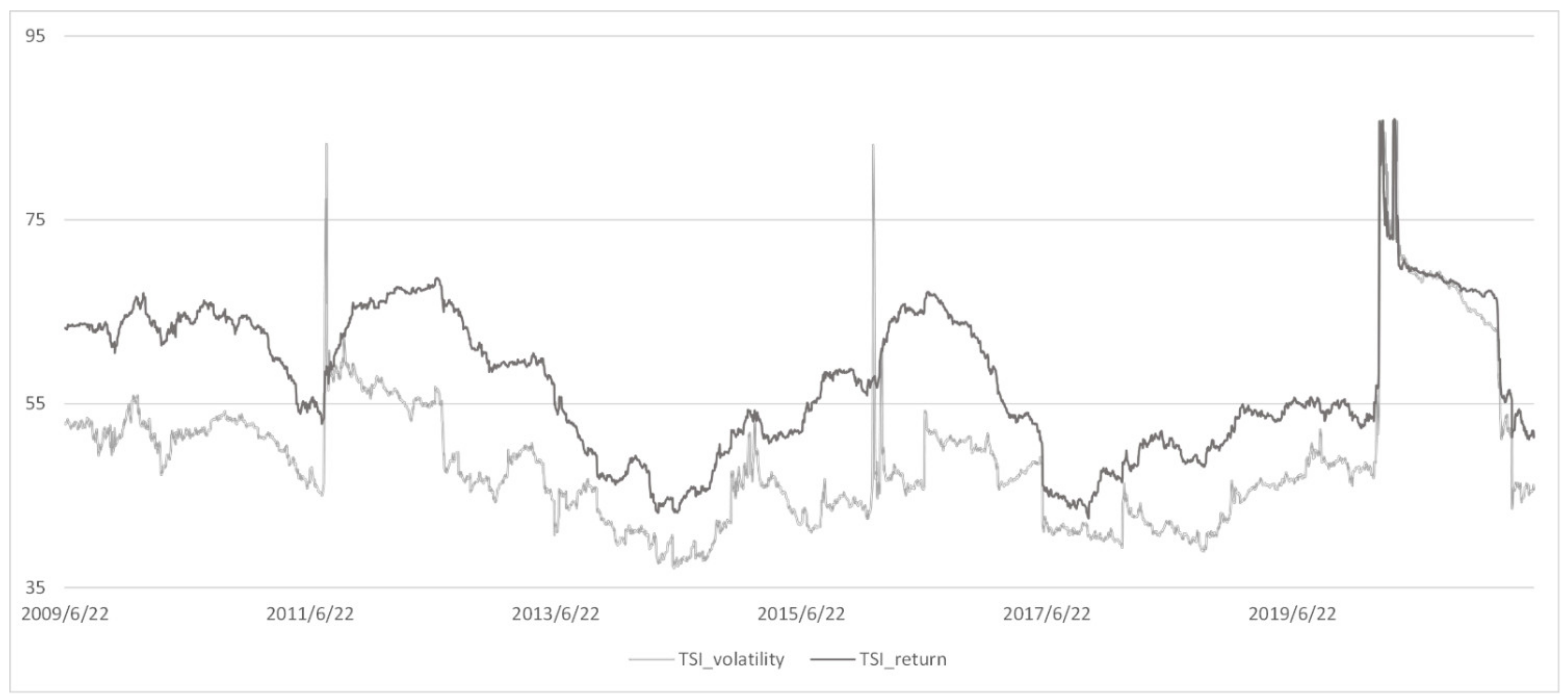
To study how the system connectedness changes over time, we introduce the rolling window method to research the connectedness of price return system and price volatility system, respectively. We select a window length of 250 observations, because 250 observations roughly correspond to one natural year. In subsequent robustness tests, we prove that the selection of window length does not change the results of the empirical study. The total spillover indices of the price return system and the price volatility system are shown in Figure 2. The date in the figure is the last day of each subsample. Taking the data corresponding to 23 June 2009 as an example, it represents the total spillover index from 25 June 2008 to 23 June 2009. Figure 2 suggests that the total spillover indices for both the return and volatility systems have time-varying features. The range of the spillover indices for both systems is relatively close and both are at a high level, which indicates a strong information spillover effect between variables. The difference is that in most cases, the total spillover index of the return system is slightly higher than that of the volatility system, and the total spillover index of the return system is smoother, while the total spillover index of the volatility system sometimes rises or falls sharply in a short period of time.
Figure 2 shows that the indices of the two systems have similar trends. From the second half of 2009 to the end of 2010, the total spillover index is at a high level, which may be caused by the global financial crisis of 2008–2009. During the financial crisis, investors in the stock market, bond market, and energy market believed that the market was full of uncertainty, and thus became more sensitive to the news they received. This leads to stronger information spillovers in the system. After that, the total spillover index experiences a short-term decline, until the second half of 2011, the index begins to climb continuously, and reaches a higher level in July 2012. The rising index at this stage may be caused by the European debt crisis from 2010 to 2012. The European Debt Crisis began with the Greek debt crisis at the end of 2009 and then spread to the entire Europe. As a result, investors were not optimistic about the prospects of the European economy, and the level of risk spillovers between markets is greatly increased. Our finding that the spillover indices increase significantly during the recession of 2007–2009 and the European debt crisis of 2010–2012 supports the view of Li and Yin, Krehlik and Barunik et al., that when financial markets are in turmoil, the interaction between commodity markets and financial markets will be dramatically enhanced [48,49]. After the European debt crisis, the spillover index shows a trend of gradual decline in the following two years.
From the second half of 2014 to the second half of 2016, there is long-term increase in the spillover index. This is because starting from the second half of 2014, global crude oil prices fell sharply due to factors such as the increase in global crude oil supply, the slowdown in crude oil demand growth, the appreciation of the US dollar, and the weakening of speculative demand. One possible explanation is that volatility in the oil market risk to financial markets. This is in line with the previous research of Salisu and Oloko, Du and He et al., that the oil market volatility will produce spillovers to the stock market [50,51]. The spillover index begins to decline in the second half of 2016 and reaches a lower level in the second half of 2017. This may be because the world economy has been recovering, but at a slower pace. Starting from the second half of 2017, the total spillover index indicates a moderate upward trend, which may be due to the overall good recovery trend of the global economy in 2017–2018.
In February 2020, the COVID-19 pandemic has gradually spread around the world, causing a huge impact on the global economy. The financial markets and commodity markets were full of uncertainty and fear, and the transmission of information between markets has become more active. The total spillover index also increases rapidly from this period and remains at a high level until early 2021. Starting in 2021, due to strong policy support, effective vaccination and the gradual recovery of economic activities, the global economy has begun to slowly recover, and the total spillover index has fallen to a low level.
To acquire more findings from the study of dynamic connectedness, we analyze the data of dynamic connectedness in the price return system and price volatility system, respectively, and the results are shown in Table 3. We calculate the expected value and standard deviation of received spillover, transmitted spillover, and net spillover for each market, respectively, as well as the percentage of net spillover when it is positive. In Table 3 Panel A and Panel B, the proportions of net connectedness of NEX, MSCI and PSE all exceed 50%, indicating that these three are net information transmitters of the system in most cases, which is also in line with the conclusion of static connectedness analysis.
The summary statistics of the pairwise connectedness between renewable energy stocks with other markets are shown in Table 4. Table 4 Panel A shows that in the price return system, the proportion of NEX as net information transmitter for PSE is only 23.44%, which means PSE is a net information transmitter to NEX in most of the time, and the change of returns in the technology stocks market have a great impact on the returns in the renewable energy stocks market. The proportions of NEX as net information transmitter to WTI and Brent reach 83.37 and 85.03%, respectively, indicating that crude oil market basically does not play a leading role in the renewable energy stocks market, which is consistent with the conclusion of our static research. As shown in Table 4 Panel B, PSE is also a net information transmitter for NEX in most cases under the price volatility system, indicating that uncertainty in the technology stocks market generates a risk spillover to the renewable energy stocks market. In the price volatility system, for crude oil markets, the percentage of NEX being a net information transmitter is slightly over 50% (56.91 and 58.47%, respectively). It shows that although renewable energy stocks have a certain leading role in the crude oil markets, the crude oil market is a key risk source that the renewable energy stocks market needs to focus on.
4.2. Connectedness Analysis in the Frequency Domain
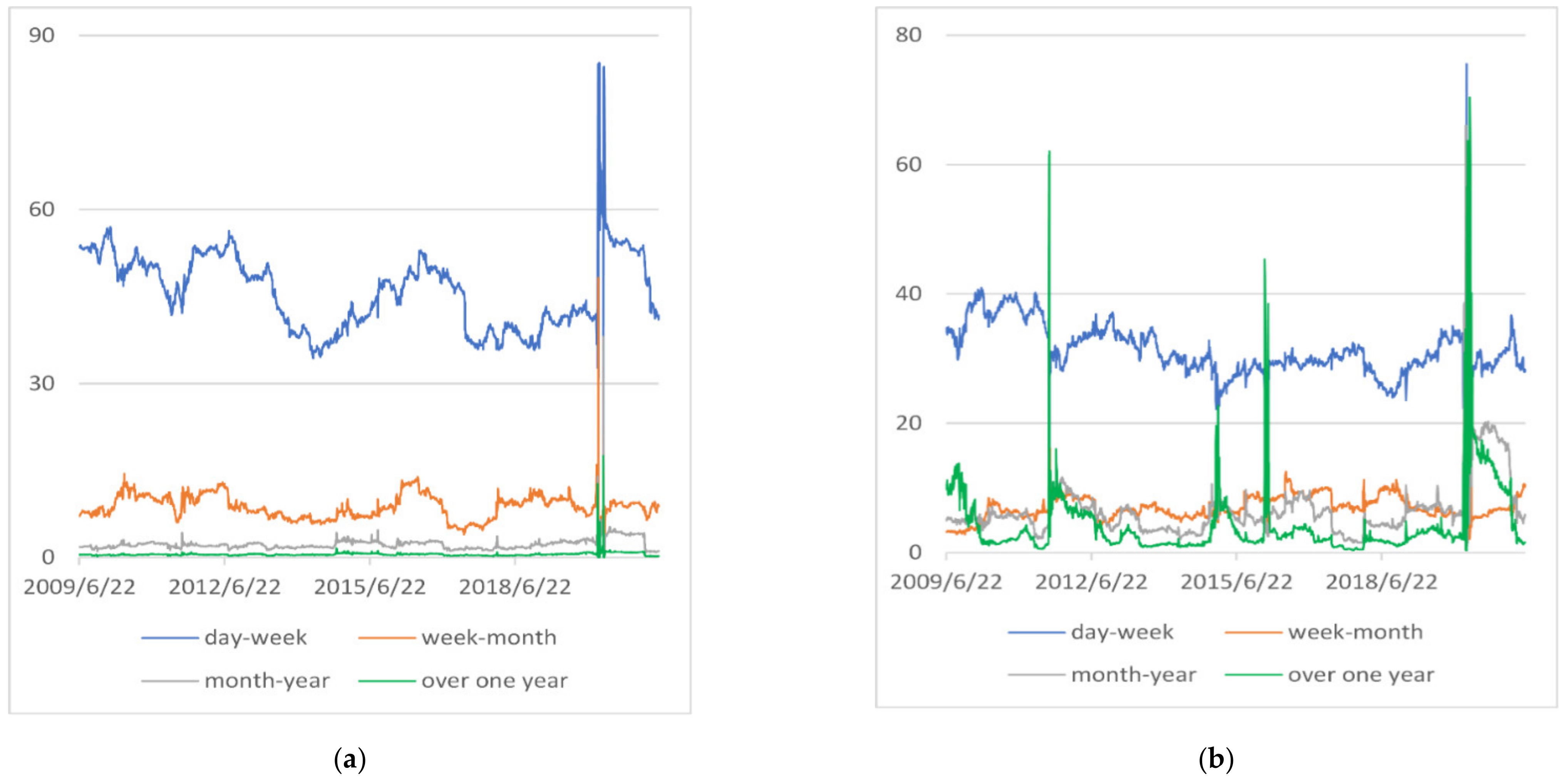
To study the frequency dynamics of the connectedness, we set four frequency bands , , , from high to low, and they correspond to time spans of one day to one week (short term), one week to one month (medium term), one month to one year (medium to long term), and over one year (long term).
4.2.1. Total Return and Volatility Connectedness
The total connectedness of return system and volatility system in different frequency bands is shown in Figure 3a and Figure 3b, respectively. We choose a rolling window with a width of 250 observations and a forecast horizon of 100 observations. As shown in Figure 4, the connectedness of the two systems in different frequency bands is time-varying. Figure 3a shows that for price return system, the connectedness in the highest frequency band () is the highest. This shows that during the full sample period, the spillovers between markets are mainly driven by information about price changes in the short term. However, the spillover index during the COVID-19 pandemic has a different situation, and we will examine this phase separately in the following. Figure 3b shows that, compared with the price return system, the connectedness gap between different frequency bands in the price volatility system is not as large as that in the price return system, and the connectedness in the price volatility system is more volatile. This suggests that information related to price volatility is more actively transmitted in the system between different markets than information related to price return. In the price volatility system, the connectedness in the highest frequency band () is the highest. There are three periods in the figure where the connectedness in , or exceeds that in . According to Figure 2, we find that these three periods are exactly the periods when the total spillover index increases substantially in a short period. Next, we will analyze these three time periods separately.
To take full advantage of the frequency decomposition method, we focus on the connectedness decomposition during the European debt crisis from 2010 to 2012, the international oil price decline from 2015 to 2016, and the COVID-19 pandemic in 2020.
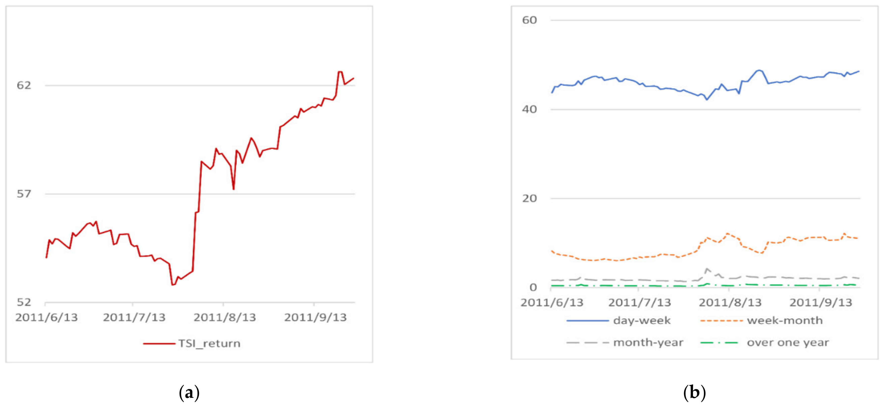
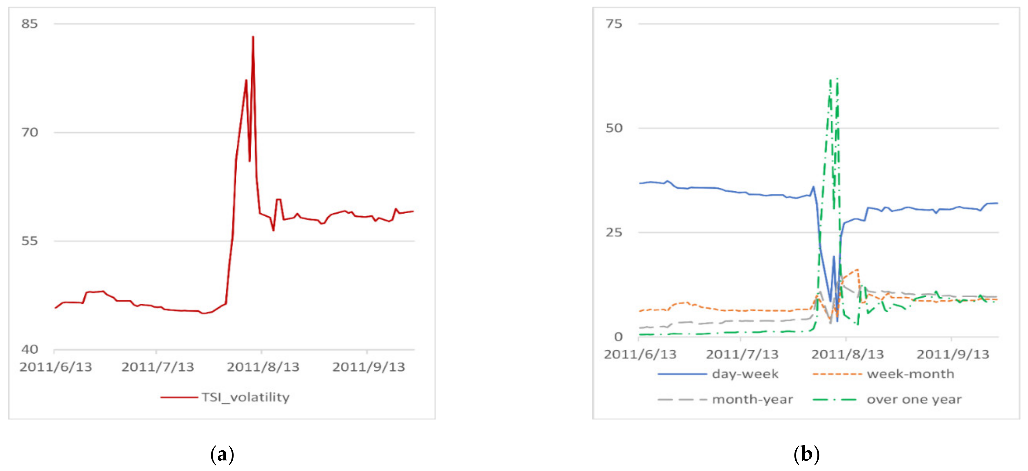
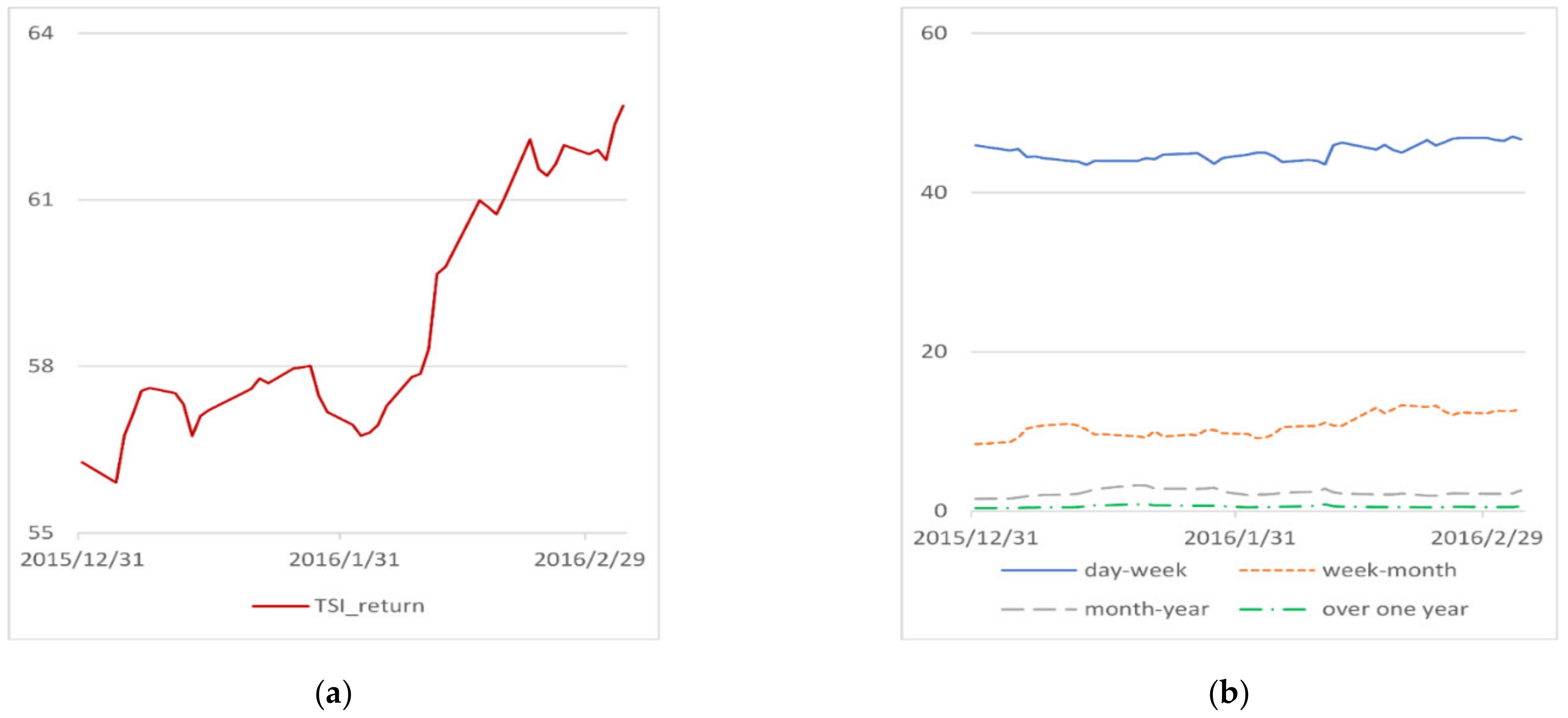
The total connectedness of the return system and the volatility system during the European debt crisis from 2010 to 2012 are shown in Figure 4 and Figure 5, respectively. Figure 4b shows that in the price return system, the connectedness at is higher than that of other bands, which indicates that during the European debt crisis, investors pay more attention to the short-term information, that is, information about price returns within a week. As shown in Figure 5b, connectedness within one year all shows varying degrees of decline, while connectedness beyond one year increases sharply. Combined with Figure 5a, we find that the growth of total connectedness during this period is mainly due to the growth of long-term spillovers. This suggests that European debt crisis has changed investors’ long-term expectations of systemic volatility.
The total connectedness of the return system and the volatility system during the international oil price decline in 2015–2016 are shown in Figure 6 and Figure 7, respectively. Figure 6b shows that in the price return system, the connectedness at is the highest. which suggests that the high-frequency price return information was a major concern for investors during the 2015–2016 international oil price decline. Figure 7b shows that in the price volatility system, the spillovers generated within one week experience two sharp declines. In the period corresponding to these two declines, spillovers generated over a period of one month to one year, or more than one year, have experienced significant increases. This indicates that the sharp increase in the total spillover index shown in Figure 7a is mainly driven by medium to long term and long-term connectedness. This may be because the uncertainty in the oil market during the oil price crash significantly increased the long-term volatility of the system.
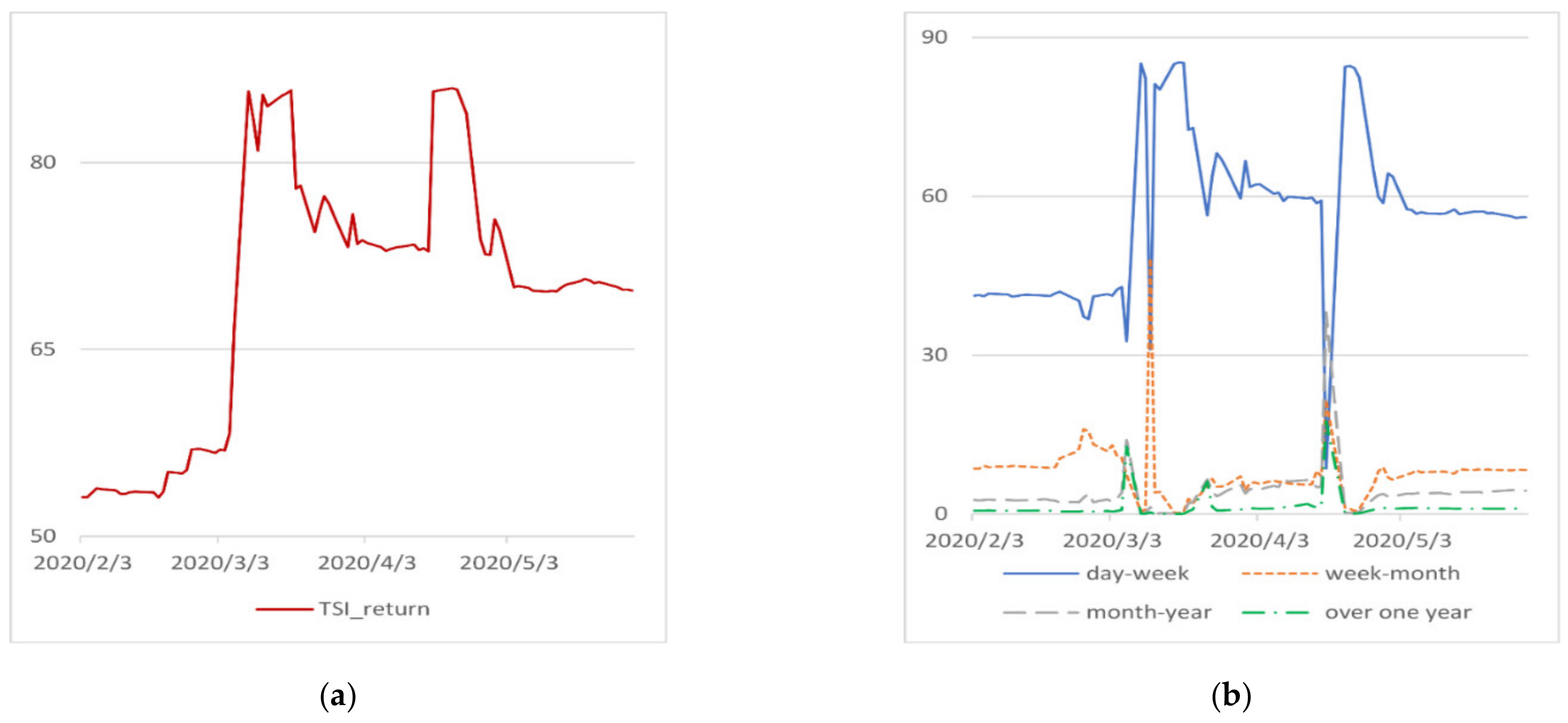
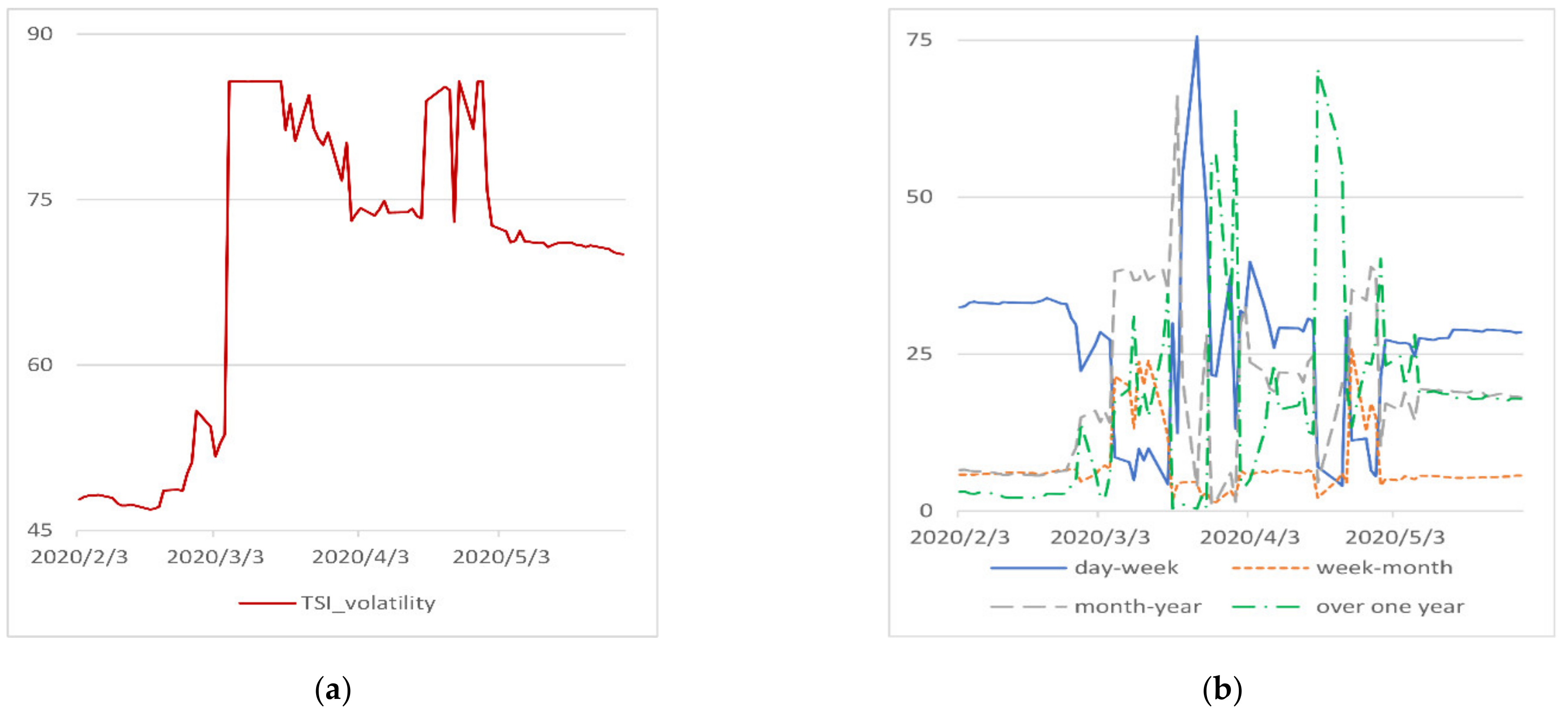
The total connectedness of the return system and the volatility system during COVID-19 pandemic are shown in Figure 8 and Figure 9, respectively. By comparing Figure 8a,b, we observe that most of the total spillovers of the price return system during this period occur within one week. As shown in Figure 8b, the spillovers generated over a period of more than a week all rise to varying degrees, which is due to the change in market investors’ expectations of price returns over a period of more than a week as a result of the impact of the pandemic. Comparing Figure 9a with Figure 9b, we see that the total spillover index experiences two increases in early March and mid-April, during which connectedness at falls significantly, while connectedness at all other bands increases to varying degrees. This shows that the increases of total spillovers in these two time periods are mainly caused by spillovers in more than one week. This is because the pandemic has had a far-reaching impact on the uncertainty of the market.
4.2.2. Net Directional Return and Volatility Connectedness
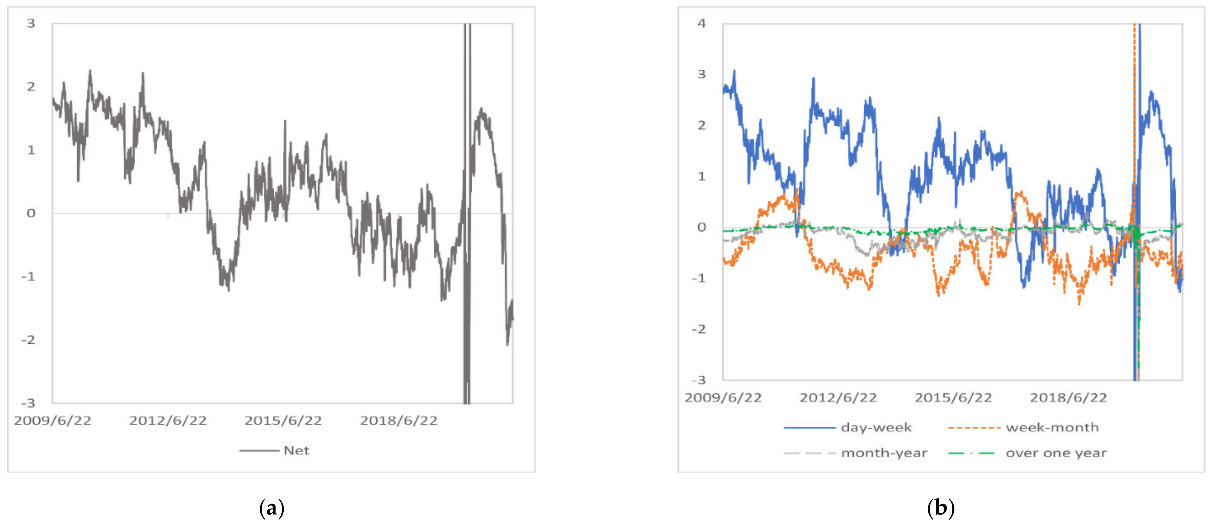
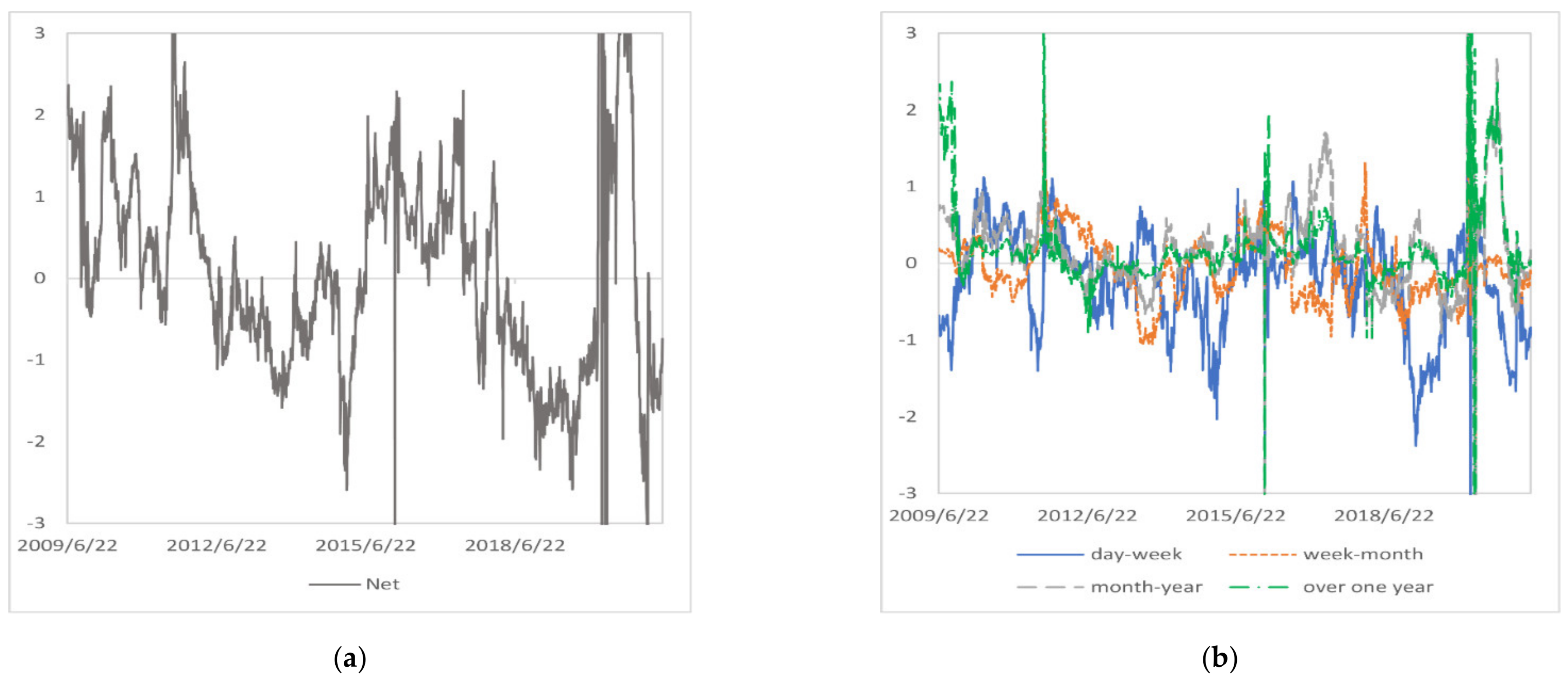
We present summary statistics on the net connectedness in price return and price volatility system in different frequency bands, as shown in Table A1. It is worth noting that in the price return system, NEX plays different roles in different frequency bands. The proportion of NEX as the net information transmitter of the system is 81.71% at , much higher than the 17.96, 21.85 and 25.46% at , and . This shows that at the high frequency band, NEX is the net information transmitter, while in other lower frequency bands, NEX is the net information receiver. By comparing Figure 10a,b, it can also be found that the net connectedness of NEX is mainly driven by short-term net connectedness. This may be because investors tend to take renewable energy stocks as a short-term investment asset, as investors are more concerned about the change in returns of renewable energy stocks within the week. In the price volatility system, NEX also plays different roles at different frequency bands. At and , the proportion of NEX as the net information transmitter of the system is 65.77 and 67.30%, respectively, while at and , the proportion of NEX as the net information transmitter of the system is 38.71 and 41.27%, respectively. By comparing Figure 11a,b, we observe that during the 2007–2009 financial crisis, European debt crisis, oil price decline and COVID-19, net connectedness is mainly driven by connectedness at , which suggests that macroeconomics or financial markets have a profound effect on the net connectedness of NEX in price volatility system.
4.2.3. Pairwise Return and Volatility Connectedness
We analyze the pairwise connectedness between variables and summarize the statistical results as shown in Table 5.
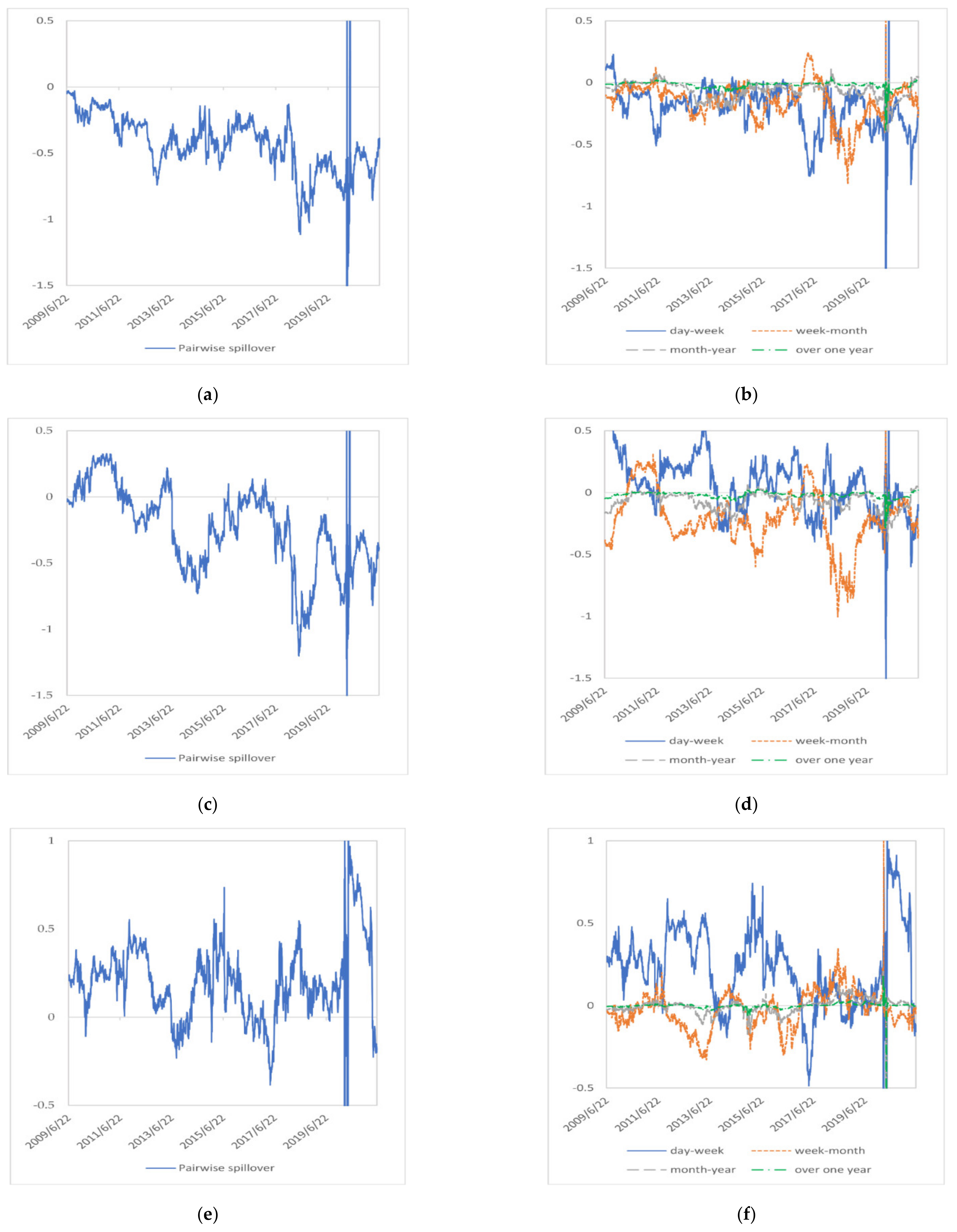
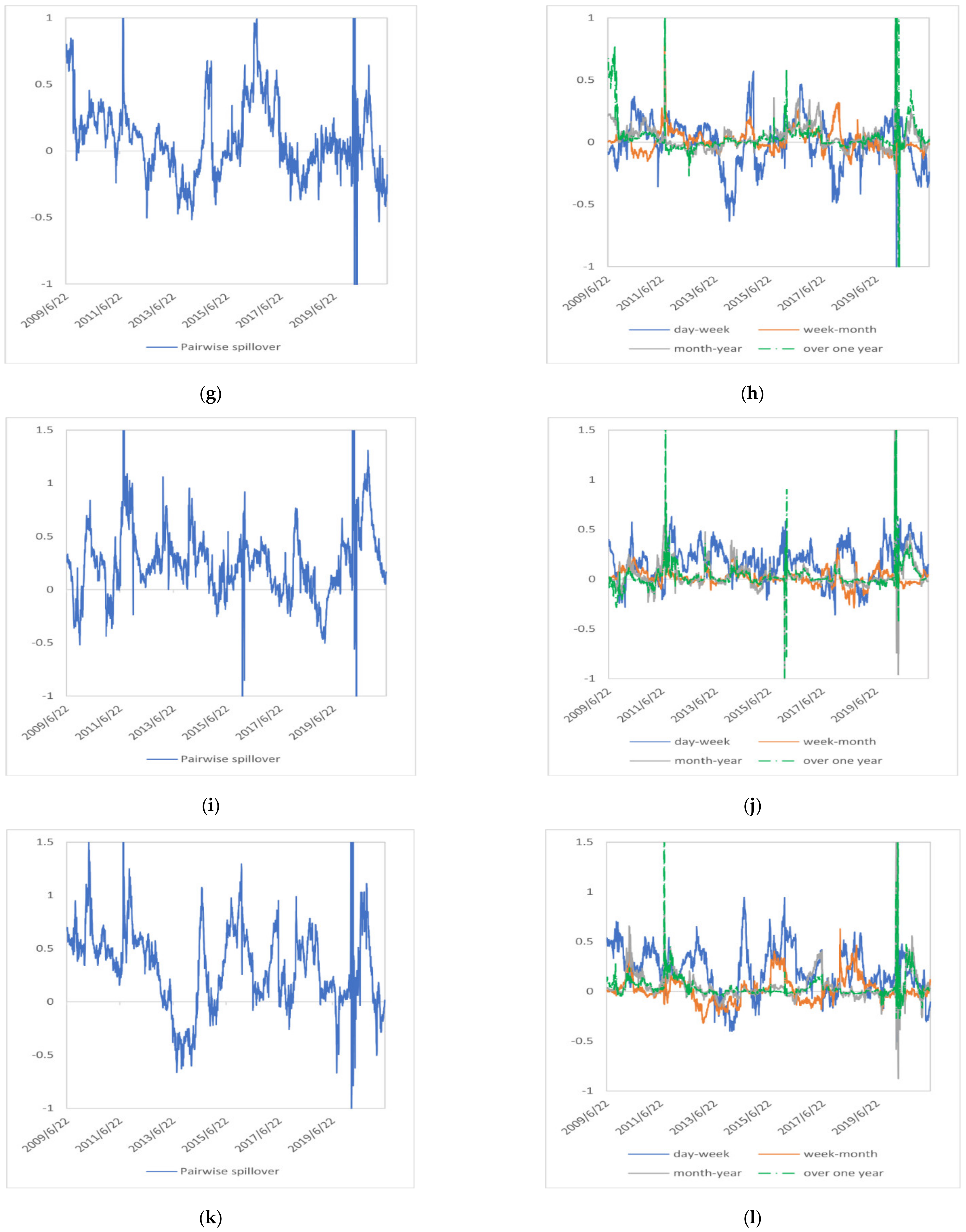
In the price return system, the pairwise connectedness and frequency decomposition between NEX and other variables are shown in Figure 12. MSCI is a net information transmitter for NEX at all frequency bands, because the price return of renewable energy stocks is closely related to the overall performance of the stock market. In the short term, NEX is mostly a net information transmitter for PSE, while in the medium and medium to long term, technology stocks are net information transmitters for renewable energy stocks. This may be because in the short term, as an investment asset, the price return information of renewable energy stocks has a greater impact on technology stocks, while in the medium to long and long term, the development of renewable energy industry depends on the development of related technologies. For WTI and Brent, in the short term, the proportion of NEX as a net information transmitter exceeds 80%, while in the medium, medium to long, and long term, the proportion of NEX as a net information transmitter reaches about 50%. This shows that in the short term, the price return of crude oil futures hardly plays a leading role in the price return of renewable energy stocks, but in the horizon of more than one week, the price of crude oil futures still has a certain influence on the price of renewable energy stocks. The connectedness between renewable energy stocks and carbon trading markets is similar to that between renewable energy stocks and crude oil futures, which means that within a week, the carbon price have a limited impact on renewable energy stocks, while over a period longer than a week, the carbon price have some impact on renewable energy stocks.
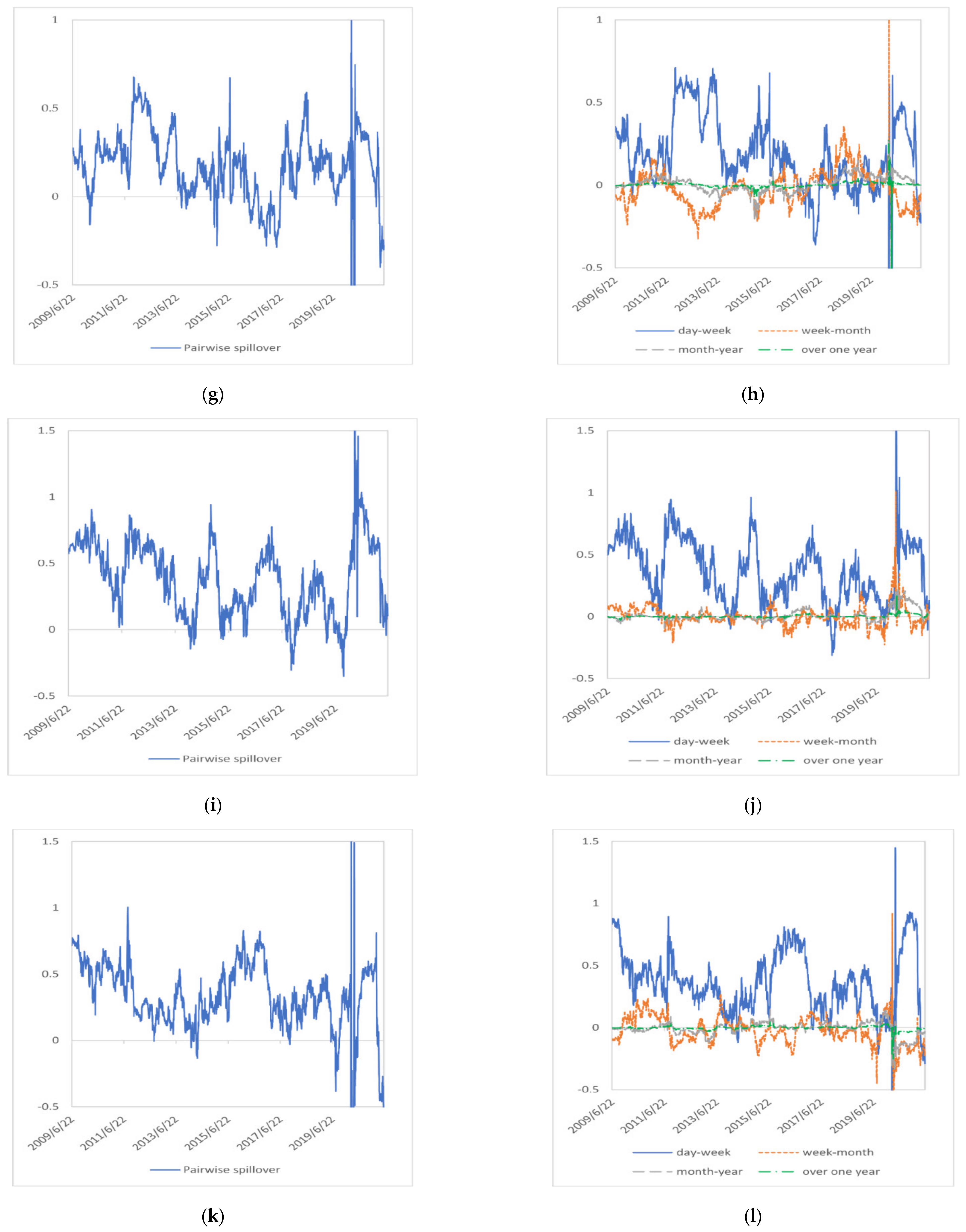
Figure 13 depicts the pairwise connectedness and frequency decomposition between NEX and other variables in a price volatility system. As shown in Table 5 Panel B, in the short term, MSCI is NEX’s net transmitter in more than 90% of the cases, and as the time horizon increases, the proportion of NEX as a net transmitter increase. This shows that with the increase of time range, the impact of the volatility of the renewable energy stocks market on the global stock market cannot be ignored. The interaction between the renewable energy stocks market and the technology stocks market is quite different in the price volatility system and the price return system. In the short term, the volatility of the renewable energy stocks market has a small impact on the technology stock market in the price volatility system. As the time horizon expands, the proportion of renewable energy stocks as net information transmitters for technology stocks gradually increases, and the proportion of NEX as net information transmitters even exceeds 50% in the time horizon of more than one month, which indicates that the uncertainty of the renewable energy stocks market has a more significant impact on technology stocks as the time horizon increases. For both WTI and Brent, the proportion of NEX as a net messenger is around 50% at all frequency bands, suggesting that the uncertainty in the crude oil market is having a non-negligible impact on the renewable energy stocks market. For the carbon trading market, the proportion of NEX as a net transmitter exceeds 80% for a time horizon of one week and is around 50% for a time horizon of more than one week, which indicatesthat the volatility of the renewable energy stocks market has an important impact on the carbon trading market.
4.3. Robustness Check
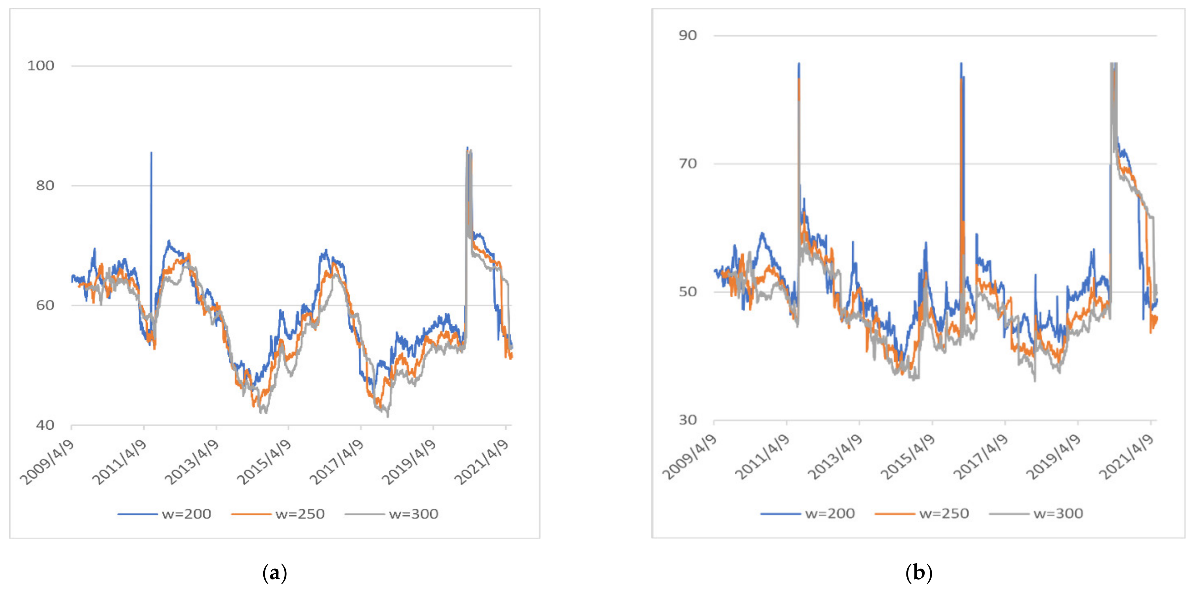
To test the robustness of our empirical results, we examine the sensitivity of the total spillover index to different rolling window widths. Figure 14a,b depict the time-varying total spillover indices for rolling window lengths of 200, 250, and 300 observations in the price return system and price volatility system, respectively. From the figures, we can see that with the increase of the window lengths, the total spillover indices lines become smoother and the values become smaller, which may be because some spillovers in the short term cannot be captured as the window lengths increase, but the time-varying trends of the total spillover indices are consistent. We conduct robustness tests on connectedness in the four frequency bands, respectively, and obtain the same results, indicating that the empirical results of this paper are unaffected by window size selection.
5. Conclusions and Discussion
The renewable energy sector has grown substantially over the past decades, which makes the renewable energy stocks become an investment asset attracting growing attention. Thus, the relationship between renewable energy stocks and other investment assets has aroused wide interest of scholars, policy makers and market investors. To obtain the frequency dynamics of spillovers between renewable energy stocks and other energy or financial assets, this paper employs the connectedness method proposed by Barunik and Krehlik (2018) to study the price return and price volatility connectedness among renewable energy stocks, global stock index, technology stocks, crude oil futures, carbon allowances, and the 10-year US Treasury note both in time and frequency domains. Through empirical research, this paper has the following main findings:
First, in the system composed of renewable energy stocks, technology stocks, crude oil futures, and carbon allowances, both price return spillovers and price volatility spillovers are high and are mainly driven by short-term (within one week) spillovers. This shows that the information about price return and price volatility in the system is transmitted quickly, and market participants process the information efficiently. On a longer time horizon (more than one week), the markets in the system may be mainly affected by its own fundamentals, rather than by prices of other markets in the system. Scholars such as Wang and Wang, Cui et al., and Umar et al., who also adopted the approach proposed by Barunik and Krehlik (2018) to study the volatility spillover in the system consisting of energy and financial markets, have different views on whether the overall risk spillover occurs mainly in the short run or in the long run [24,52,53]. We believe that this may be related to the type of energy sources selected and the different regions studied. However, these studies all point out that the overall volatility spillover level of the energy market or financial market increases significantly during periods of economic or financial market turbulence, which is consistent with the findings of this paper.
Second, we find something new about renewable energy’s relationship with crude oil or technology stocks, respectively. We find that we cannot simply generalize to which asset renewable energy stocks are more strongly associated with but should instead consider the frequency dynamics of the relationship between assets. Our study in the time domain has similar finding to that of Sadorsky, Ahmad, Inchauspe et al. in that technology stocks have a more significant impact on renewable energy stocks compared to crude oil [12,13,14]. However, through the study in the frequency domain, we find that renewable energy stocks show a more complex relationship with the two at different time scales.
- i.
- In the price return system, only in the short term, renewable energy has a significant spillover effect on the price of crude oil. In longer time scales, the impact of crude oil on renewable energy stocks is enhanced. In the price volatility system, crude oil has certain influence on the risk of renewable energy stock market in all frequency bands, which means that renewable energy stock investors need to pay attention to the volatility of crude oil prices and adjust the asset allocation in their portfolios in a timely manner. In addition, policy makers should improve the price mechanism of the crude oil market to prevent the violent fluctuation of crude oil prices from having a huge impact on the renewable energy financial market.
- ii.
- In the price return system, renewable energy stocks have a significant spillover effect on technology stocks in the short term, while technology stocks have a significant spillover effect on the renewable energy over a time scale of more than a week. This may mean that the long-term return of renewable energy is more strongly influenced by the return of the technology industry, and it’s an effective way to achieve sustainable development of the renewable energy industry by promoting the progress of science and technology. In the price volatility system, only in the short term, technology stocks have a significant impact on renewable energy stocks. In longer time scales, the dominant role of technology stocks diminishes. For short-term investors, including technology stocks and renewable energy stocks in the same portfolio may increase investment risk.
Third, only in the short term, renewable energy stock prices have significant price return spillover effect and price volatility spillover effect on carbon allowance prices. In longer terms, renewable energy stock prices have limited influence on carbon allowances prices while other factors such as energy prices, climate and policies may have a greater impact. Therefore, short-term investors in carbon markets should pay more attention to renewable energy stocks, while other investors may need to focus more on other energy prices, climate, or policies. In addition, over a time scale of more than a week, the carbon price has a certain impact on the return and risk of renewable energy stocks.
There are few studies on the relationship between the price of carbon allowances and the volatility of renewable energy stock prices, such as those by Dutta et al., Xia et al., Lin and Chen and Jiang et al., among which only Jiang et al. consider the time scale factor. Different from the wavelet method used by Jiang et al., by introducing a frequency-dependent connectedness network model, we not only consider different time scales, but also study the dynamic relationship between carbon prices and renewable energy stock prices.
Fourth, during the turmoil in the financial market, macro economy or energy market, the price return and price volatility spillover effect of the system composed of renewable energy stocks and other assets will become stronger, especially the volatility spillover effect. This is consistent with previous finding that major crisis events enhance the risk transmission between energy and financial markets [24,30,52,53]. During the European debt crisis, the international oil price decline and the COVID-19 pandemic, the total volatility spillover of the system has increased substantially, which is not caused by spillovers within one week, but by spillovers in longer time scales. This suggests that risk transmission between renewable energy stocks and other assets has been profoundly affected.
This research has made new findings on the relationship between the renewable energy and investment assets such as technology stocks, crude oil futures and carbon allowances, which can not only provide reference for investors to manage risks and optimize asset allocation strategies, but also provide suggestions for policy makers to promote the development of renewable energy industry and maintain market stability. The limitation of this paper is that it only analyzes the spillover results between renewable energy stocks and other investment assets in different frequency domains, and lacks research on the hedging ratio between different assets, which will be the focus of our further research.
Author Contributions
D.N. put forward the idea of the article, conducted the empirical analysis, and wrote the original manuscript; Y.L. gave some important support and guidance; X.L. provided some key advice and revised the manuscript; X.Z. made some contributions to the original manuscript; F.Z. offered some advice and help. All authors have read and agreed to the published version of the manuscript.
Funding
This research was supported by Beijing Natural Science Foundation (9224037) and Fundamental Research Funds for the Central Universities (2022FR004).
Institutional Review Board Statement
Not applicable.
Informed Consent Statement
Not applicable.
Data Availability Statement
The study did not report any data.
Conflicts of Interest
The authors declare no conflict of interest.
Appendix A

Table A1.
Summary statistics of net pairwise connectedness between NEX and other variables.
| Mean | Std. Dev. | Proportion | ||||||||||
|---|---|---|---|---|---|---|---|---|---|---|---|---|
| Panel A: price return system | ||||||||||||
| day-week | week-month | month-year | over one year | day-week | week-month | month-year | over one year | day-week | week-month | month-year | over one year | |
| NEX | 1.00 | −0.44 | −0.13 | −0.03 | 1.01 | 0.49 | 0.19 | 0.07 | 81.71% | 17.96% | 21.85% | 25.46% |
| MSCI | 2.18 | 0.15 | 0.10 | 0.03 | 1.09 | 0.31 | 0.20 | 0.09 | 99.80% | 65.80% | 72.08% | 73.41% |
| PSE | 0.52 | 0.46 | 0.16 | 0.04 | 0.94 | 0.44 | 0.18 | 0.07 | 73.44% | 86.75% | 90.90% | 86.85% |
| WTI | −0.31 | 0.09 | 0.02 | 0.01 | 1.52 | 0.38 | 0.50 | 0.23 | 40.07% | 63.31% | 57.24% | 58.80% |
| Brent | −0.09 | 0.00 | −0.05 | −0.01 | 0.92 | 0.29 | 0.18 | 0.08 | 56.74% | 48.54% | 42.86% | 42.20% |
| EUA | −1.66 | −0.19 | −0.08 | −0.02 | 1.04 | 0.31 | 0.24 | 0.08 | 1.23% | 24.07% | 34.59% | 37.72% |
| 10 YTN | −1.63 | −0.07 | −0.03 | −0.01 | 1.18 | 0.41 | 0.25 | 0.08 | 2.16% | 40.54% | 41.24% | 44.09% |
| Panel B: price volatility system | ||||||||||||
| day-week | week-month | month-year | over one year | day-week | week-month | month-year | over one year | day-week | week-month | month-year | over one year | |
| NEX | −0.23 | −0.07 | 0.21 | 0.20 | 0.63 | 0.43 | 0.69 | 0.77 | 38.71% | 41.27% | 65.77% | 67.30% |
| MSCI | 1.20 | 0.26 | 0.32 | 0.21 | 0.70 | 0.33 | 0.64 | 0.59 | 93.86% | 82.64% | 77.62% | 77.46% |
| PSE | 0.50 | −0.05 | −0.08 | −0.03 | 0.64 | 0.31 | 0.54 | 0.55 | 78.15% | 39.31% | 45.92% | 49.20% |
| WTI | 0.08 | 0.09 | 0.00 | 0.00 | 0.80 | 0.50 | 0.93 | 1.15 | 55.38% | 64.24% | 44.65% | 46.68% |
| Brent | 0.07 | −0.07 | −0.11 | −0.10 | 0.67 | 0.33 | 0.47 | 0.68 | 57.40% | 43.29% | 48.57% | 45.32% |
| EUA | −0.70 | −0.08 | −0.16 | −0.09 | 0.93 | 0.32 | 0.63 | 0.96 | 18.43% | 37.78% | 36.19% | 37.98% |
| 10 YTN | −0.92 | −0.09 | −0.20 | −0.19 | 0.66 | 0.34 | 0.63 | 0.56 | 10.33% | 42.70% | 39.74% | 34.03% |
Note: “Proportion” refers to the share of positive value of net pairwise connectedness between NEX with another variable in the total net pairwise connectedness between these two variables.
References
- The Renewables 2019 Global Status Report. Available online: https://www.ren21.net/gsr-2019/chapters/chapter_01/chapter_01/ (accessed on 6 October 2021).
- The 2020 Edition of Energy Outlook. Available online: https://www.bp.com/content/dam/bp/business-sites/en/global/corporate/pdfs/energy-economics/energy-outlook/bp-energy-outlook-2020.pdf (accessed on 6 October 2021).
- The 2019 Edition of World Energy Outlook. Available online: https://iea.blob.core.windows.net/assets/98909c1b-aabc-4797-9926-35307b418cdb/WEO2019-free.pdf (accessed on 7 October 2021).
- Henriques, I.; Sadorsky, P. Oil Prices and the Stock Prices of Alternative Energy Companies. Energy Econ. 2008, 30, 998–1010. [Google Scholar] [CrossRef]
- Kumar, S.; Managi, S.; Matsuda, A. Stock Prices of Clean Energy Firms, Oil and Carbon Markets: A Vector Autoregressive Analysis. Energy Econ. 2012, 34, 215–226. [Google Scholar] [CrossRef]
- Ahmad, W.; Sadorsky, P.; Sharma, A. Optimal Hedge Ratios for Clean Energy Equities. Econ. Model. 2018, 72, 278–295. [Google Scholar] [CrossRef]
- Reboredo, J.C.; Ugolini, A. The Impact of Energy Prices on Clean Energy Stock Prices. A Multivariate Quantile Dependence Approach. Energy Econ. 2018, 76, 136–152. [Google Scholar] [CrossRef]
- Song, Y.; Ji, Q.; Du, Y.J.; Geng, J.B. The Dynamic Dependence of Fossil Energy, Investor Sentiment and Renewable Energy Stock Markets. Energy Econ. 2019, 84, 104564. [Google Scholar] [CrossRef]
- Managi, S.; Okimoto, T. Does the Price of Oil Interact with Clean Energy Prices in the Stock Market? Japan World Econ. 2013, 27, 1–9. [Google Scholar] [CrossRef] [Green Version]
- Paiva, A.S.S.; Rivera-Castro, M.A.; Andrade, R.F.S. DCCA Analysis of Renewable and Conventional Energy Prices. Phys. A Stat. Mech. Its Appl. 2018, 490, 1408–1414. [Google Scholar] [CrossRef]
- Reboredo, J.C.; Rivera-Castro, M.A.; Ugolini, A. Wavelet-Based Test of Co-Movement and Causality between Oil and Renewable Energy Stock Prices. Energy Econ. 2017, 61, 241–252. [Google Scholar] [CrossRef]
- Sadorsky, P. Correlations and Volatility Spillovers between Oil Prices and the Stock Prices of Clean Energy and Technology Companies. Energy Econ. 2012, 34, 248–255. [Google Scholar] [CrossRef]
- Ahmad, W. On the Dynamic Dependence and Investment Performance of Crude Oil and Clean Energy Stocks. Res. Int. Bus. Financ. 2017, 42, 376–389. [Google Scholar] [CrossRef]
- Inchauspe, J.; Ripple, R.D.; Trück, S. The Dynamics of Returns on Renewable Energy Companies: A State-Space Approach. Energy Econ. 2015, 48, 325–335. [Google Scholar] [CrossRef]
- Zhang, G.; Du, Z. Co-Movements among the Stock Prices of New Energy, High-Technology and Fossil Fuel Companies in China. Energy 2017, 135, 249–256. [Google Scholar] [CrossRef]
- Tiwari, A.K.; Nasreen, S.; Hammoudeh, S.; Selmi, R. Dynamic Dependence of Oil, Clean Energy and the Role of Technology Companies: New Evidence from Copulas with Regime Switching. Energy 2021, 220, 119590. [Google Scholar] [CrossRef]
- Ferrer, R.; Shahzad, S.J.H.; López, R.; Jareño, F. Time and Frequency Dynamics of Connectedness between Renewable Energy Stocks and Crude Oil Prices. Energy Econ. 2018, 76, 1–20. [Google Scholar] [CrossRef]
- Bondia, R.; Ghosh, S.; Kanjilal, K. International Crude Oil Prices and the Stock Prices of Clean Energy and Technology Companies: Evidence from Non-Linear Cointegration Tests with Unknown Structural Breaks. Energy 2016, 101, 558–565. [Google Scholar] [CrossRef]
- Kocaarslan, B.; Soytas, U. Asymmetric Pass-through between Oil Prices and the Stock Prices of Clean Energy Firms: New Evidence from a Nonlinear Analysis. Energy Rep. 2019, 5, 117–125. [Google Scholar] [CrossRef]
- Dutta, A.; Bouri, E.; Noor, H. Return and Volatility Linkages between CO 2 Emission and Clean Energy Stock Prices. Energy 2020, 164, 803–810. [Google Scholar] [CrossRef]
- Xia, T.; Ji, Q.; Zhang, D.; Han, J. Asymmetric and Extreme Influence of Energy Price Changes on Renewable Energy Stock Performance. J. Clean. Prod. 2019, 241, 118338. [Google Scholar] [CrossRef]
- Lin, B.; Chen, Y. Dynamic Linkages and Spillover Effects between CET Market, Coal Market and Stock Market of New Energy Companies: A Case of Beijing CET Market in China. Energy 2019, 172, 1198–1210. [Google Scholar] [CrossRef]
- Jiang, C.; Wu, Y.; Li, X.; Li, X. Time-Frequency Connectedness between Coal Market Prices, New Energy Stock Prices and CO2 Emissions Trading Prices in China. Sustainability 2020, 12, 2823. [Google Scholar] [CrossRef] [Green Version]
- Wang, X.; Wang, Y. Volatility Spillovers between Crude Oil and Chinese Sectoral Equity Markets: Evidence from a Frequency Dynamics Perspective. Energy Econ. 2019, 80, 995–1009. [Google Scholar] [CrossRef]
- Diebold, F.X.; Yilmaz, K. On the Network Topology of Variance Decompositions: Measuring the Connectedness of Financial Firms. J. Econom. 2014, 182, 119–134. [Google Scholar] [CrossRef] [Green Version]
- Baruník, J.; Křehlík, T. Measuring the Frequency Dynamics of Financial Connectedness and Systemic Risk. J. Financ. Econom. 2018, 16, 271–296. [Google Scholar] [CrossRef]
- Kodres, L.E.; Pritsker, M. A Rational Expectations Model of Financial Contagion. J. Financ. 2002, 57, 769–799. [Google Scholar] [CrossRef] [Green Version]
- Acharya, V.V.; Pedersen, L.H. Asset Pricing with Liquidity Risk. J. Financ. Econ. 2005, 77, 375–410. [Google Scholar] [CrossRef] [Green Version]
- Tan, X.; Sirichand, K.; Vivian, A.; Wang, X. How Connected Is the Carbon Market to Energy and Financial Markets? A Systematic Analysis of Spillovers and Dynamics. Energy Econ. 2020, 90, 104870. [Google Scholar] [CrossRef]
- Zhang, D. Oil Shocks and Stock Markets Revisited: Measuring Connectedness from a Global Perspective. Energy Econ. 2017, 62, 323–333. [Google Scholar] [CrossRef]
- Aromi, D.; Clements, A. Spillovers between the Oil Sector and the S&P500: The Impact of Information Flow about Crude Oil. Energy Econ. 2019, 81, 187–196. [Google Scholar] [CrossRef]
- Maghyereh, A.I.; Awartani, B.; Bouri, E. The Directional Volatility Connectedness between Crude Oil and Equity Markets: New Evidence from Implied Volatility Indexes. Energy Econ. 2016, 57, 78–93. [Google Scholar] [CrossRef] [Green Version]
- Ma, Y.R.; Zhang, D.; Ji, Q.; Pan, J. Spillovers between Oil and Stock Returns in the US Energy Sector: Does Idiosyncratic Information Matter? Energy Econ. 2019, 81, 536–544. [Google Scholar] [CrossRef]
- Apergis, N.; Baruník, J.; Lau, M.C.K. Good Volatility, Bad Volatility: What Drives the Asymmetric Connectedness of Australian Electricity Markets? Energy Econ. 2017, 66, 108–115. [Google Scholar] [CrossRef]
- Zhang, D.; Ji, Q.; Kutan, A.M. Dynamic Transmission Mechanisms in Global Crude Oil Prices: Estimation and Implications. Energy 2019, 175, 1181–1193. [Google Scholar] [CrossRef]
- Restrepo, N.; Uribe, J.M.; Manotas, D. Financial Risk Network Architecture of Energy Firms. Appl. Energy 2018, 215, 630–642. [Google Scholar] [CrossRef]
- Koop, G.; Pesaran, M.H.; Potter, S.M. Impulse Response Analysis in Nonlinear Multivariate Models. J. Econom. 1996, 74, 119–147. [Google Scholar] [CrossRef]
- Pesaran, H.H.; Shin, Y. Capital Taxation and Production Efficiency in an Open Economy. Econ. Lett. 1999, 62, 85–90. [Google Scholar] [CrossRef]
- The Index Report of the WilderHill New Energy Global Innovation Index (NEX). Available online: https://cleanenergyindex.com/pdf/NEX%20for%20website%20for%20Start%20of%20Q2%202021.pdf (accessed on 22 October 2021).
- The Website of Intercontinental Exchange (ICE). Available online: https://www.theice.com/publicdocs/data/NYSE_Arca_Tech_100_Index_Methodology.pdf (accessed on 22 October 2021).
- The Website of the MSCI World Index. Available online: https://www.msci.com/documents/10199/149ed7bc-316e-4b4c-8ea4-43fcb5bd6523 (accessed on 29 October 2021).
- The Website of the MSCI World Index. Available online: https://www.msci.com/developed-markets (accessed on 22 October 2021).
- Ciner, C.; Gurdgiev, C.; Lucey, B.M. Hedges and Safe Havens: An Examination of Stocks, Bonds, Gold, Oil and Exchange Rates. Int. Rev. Financ. Anal. 2013, 29, 202–211. [Google Scholar] [CrossRef]
- Antonakakis, N.; Cunado, J.; Filis, G.; Gabauer, D.; Perez, F.; Gracia, D. Oil Volatility, Oil and Gas Firms and Portfolio Diversification. Energy Econ. 2018, 70, 499–515. [Google Scholar] [CrossRef] [Green Version]
- Wang, G.; Xie, C.; Jiang, Z.; Stanley, H.E. Who Are the Net Senders and Recipients of Volatility Spillovers in China ’ s Financial Markets ? Financ. Res. Lett. 2016, 18, 255–262. [Google Scholar] [CrossRef]
- Antonakakis, N.; Kizys, R. International Review of Financial Analysis Dynamic Spillovers between Commodity and Currency Markets. Int. Rev. Financ. Anal. 2015, 41, 303–319. [Google Scholar] [CrossRef] [Green Version]
- Berta, N.; Gautherat, E.; Gun, O. Transactions in the European Carbon Market: A Bubble of Compliance in a Whirlpool of Speculation. Cambridge J. Econ. 2017, 41, 575–593. [Google Scholar] [CrossRef] [Green Version]
- Li, L.; Yin, L.; Zhou, Y. Exogenous Shocks and the Spillover Effects between Uncertainty and Oil Price. Energy Econ. 2016, 54, 224–234. [Google Scholar] [CrossRef]
- Krehlik, T.; Barunik, J. Cyclical Properties of Supply-Side and Demand-Side Shocks in Oil-Based Commodity Markets. Energy Econ. 2017, 65, 208–218. [Google Scholar] [CrossRef] [Green Version]
- Salisu, A.A.; Oloko, T.F. Modeling Oil Price-US Stock Nexus: A VARMA-BEKK-AGARCH Approach. Energy Econ. 2015, 50, 1–12. [Google Scholar] [CrossRef]
- Du, L.; He, Y. Extreme Risk Spillovers between Crude Oil and Stock Markets. Energy Econ. 2015, 51, 455–465. [Google Scholar] [CrossRef]
- Cui, J.; Goh, M.; Li, B.; Zou, H. Dynamic Dependence and Risk Connectedness among Oil and Stock Markets: New Evidence from Time-Frequency Domain Perspectives. Energy 2021, 216, 119302. [Google Scholar] [CrossRef]
- Umar, M.; Farid, S.; Naeem, M.A. Time-Frequency Connectedness among Clean-Energy Stocks and Fossil Fuel Markets: Comparison between Financial, Oil and Pandemic Crisis. Energy 2022, 240, 122702. [Google Scholar] [CrossRef]
Figure 1.
The net pairwise connectedness over the full sample. (a) Price Return System. (b) Price Volatility System. (Note: In the figure, blue nodes represent net information receivers, and orange nodes represent net information transmitters. The heavier the color is, the stronger the overflow is. The bands between the nodes represent the direction of pairwise connectedness, with orange representing the outflow of spillovers and blue representing the inflow of spillovers. If the width of the band is larger, the connectedness is higher.).

Figure 2.
Total connectedness with rolling windows in price return system and price volatility system.
Figure 2.
Total connectedness with rolling windows in price return system and price volatility system.

Figure 3.
Total connectedness at different frequency bands in price return system and price volatility system. (a) Price Return System. (b) Price Volatility System.
Figure 3.
Total connectedness at different frequency bands in price return system and price volatility system. (a) Price Return System. (b) Price Volatility System.

Figure 4.
Total spillover of the price return system during the European debt crisis. (a) total return spillover. (b) frequency decomposition of return spillover.
Figure 4.
Total spillover of the price return system during the European debt crisis. (a) total return spillover. (b) frequency decomposition of return spillover.

Figure 5.
Total spillover of the price volatility system during the European debt crisis. (a) total volatility spillover. (b) frequency decomposition of volatility spillover.
Figure 5.
Total spillover of the price volatility system during the European debt crisis. (a) total volatility spillover. (b) frequency decomposition of volatility spillover.

Figure 6.
Total spillover of the price return system during the 2015–2016 oil price decline. (a) total return spillover. (b) frequency decomposition of return spillover.
Figure 6.
Total spillover of the price return system during the 2015–2016 oil price decline. (a) total return spillover. (b) frequency decomposition of return spillover.

Figure 7.
Total spillover of the price volatility system during the 2015–2016 oil price decline. (a) total volatility spillover. (b) frequency decomposition of volatility spillover.
Figure 7.
Total spillover of the price volatility system during the 2015–2016 oil price decline. (a) total volatility spillover. (b) frequency decomposition of volatility spillover.

Figure 8.
Total spillover of the price return system during COVID-19. (a) total return spillover. (b) frequency decomposition of return spillover.
Figure 8.
Total spillover of the price return system during COVID-19. (a) total return spillover. (b) frequency decomposition of return spillover.

Figure 9.
Total spillover of the price volatility system during COVID-19. (a) total volatility spillover. (b) frequency decomposition of volatility spillover.
Figure 9.
Total spillover of the price volatility system during COVID-19. (a) total volatility spillover. (b) frequency decomposition of volatility spillover.

Figure 10.
Net directional connectedness of NEX in the price return system. (a) net directional connectedness. (b) frequency decomposition of net connectedness.
Figure 10.
Net directional connectedness of NEX in the price return system. (a) net directional connectedness. (b) frequency decomposition of net connectedness.

Figure 11.
Net directional connectedness of NEX in the price volatility system. (a) net directional connectedness. (b) frequency decomposition of net connectedness.
Figure 11.
Net directional connectedness of NEX in the price volatility system. (a) net directional connectedness. (b) frequency decomposition of net connectedness.

Figure 12.
Pairwise connectedness between NEX and other variables in price return system. (a) pairwise connectedness between NEX and MSCI. (b) frequency decomposition of pairwise connectedness between NEX and MSCI. (c) pairwise connectedness between NEX and PSE. (d) frequency decomposition of pairwise connectedness between NEX and PSE. (e) pairwise connectedness between NEX and WTI. (f) frequency decomposition of pairwise connectedness between NEX and WTI. (g) pairwise connectedness between NEX and Brent. (h) frequency decomposition of pairwise connectedness between NEX and Brent. (i) pairwise connectedness between NEX and EUA. (j) frequency decomposition of pairwise connectedness between NEX and EUA. (k) pairwise connectedness between NEX and 10YTN. (l) frequency decomposition of pairwise connectedness between NEX and 10YTN.


Figure 13.
Pairwise connectedness between NEX and other variables in price volatility system. (a) pairwise connectedness between NEX and MSCI. (b) frequency decomposition of pairwise connectedness between NEX and MSCI. (c) pairwise connectedness between NEX and PSE. (d) frequency decomposition of pairwise connectedness between NEX and PSE. (e) pairwise connectedness between NEX and WTI. (f) frequency decomposition of pairwise connectedness between NEX and WTI. (g) pairwise connectedness between NEX and Brent. (h) frequency decomposition of pairwise connectedness between NEX and Brent. (i) pairwise connectedness between NEX and EUA. (j) frequency decomposition of pairwise connectedness between NEX and EUA. (k) pairwise connectedness between NEX and 10YTN. (l) frequency decomposition of pairwise connectedness between NEX and 10YTN.


Figure 14.
Dynamic total connectedness with window widths of 200, 250, 300 observations. (a) Price Return System. (b) Price Volatility System.
Figure 14.
Dynamic total connectedness with window widths of 200, 250, 300 observations. (a) Price Return System. (b) Price Volatility System.

Table 1.
Descriptive statistics of price returns and price volatilities.
| NEX | MSCI | PSE | WTI | Brent | EUA | 10 YTN | |
|---|---|---|---|---|---|---|---|
| Panel A: Descriptive statistics of price returns | |||||||
| Mean | 0.003143 | 0.022832 | 0.054781 | −0.01991 | −0.0189 | 0.020422 | −0.03222 |
| Median | 0.084921 | 0.076576 | 0.107949 | 0.06152 | 0.060356 | 0 | −0.0912 |
| Max. | 12.07055 | 9.096657 | 10.0988 | 31.96337 | 19.0774 | 23.92297 | 40.59273 |
| Min. | −12.5407 | −10.4412 | −12.7364 | −60.1676 | −37.3399 | −43.2421 | −34.1459 |
| Std. Dev. | 1.555478 | 1.136851 | 1.379505 | 3.022231 | 2.485705 | 3.171374 | 3.037656 |
| Skewness | −0.59983 | −0.81959 | −0.4746 | −2.22029 | −1.3013 | −0.8433 | 0.157663 |
| Kurtosis | 11.82942 | 15.47495 | 11.83082 | 66.39399 | 27.25795 | 18.09607 | 34.4649 |
| Jarque-Bera | 10,788.19 | 21,510.56 | 10,718.41 | 548,733.5 | 80,875.71 | 31,351.25 | 134,535.2 |
| Panel B: Descriptive statistics of price volatilities | |||||||
| Mean | 1.026961 | 0.720181 | 0.921661 | 1.815187 | 1.615483 | 2.181937 | 1.987256 |
| Median | 0.691197 | 0.464433 | 0.623592 | 1.205132 | 1.037256 | 1.583906 | 1.449854 |
| Max. | 12.54068 | 10.44119 | 12.73636 | 60.16758 | 37.33993 | 43.24209 | 40.59273 |
| Min. | 0 | 0.000229 | 0 | 0 | 0 | 0 | 0 |
| Std. Dev. | 1.168139 | 0.879848 | 1.027773 | 2.41627 | 1.889048 | 2.301244 | 2.297389 |
| Skewness | 3.29492 | 3.788933 | 3.218894 | 7.933581 | 4.88873 | 3.998018 | 6.243861 |
| Kurtosis | 20.35099 | 26.07892 | 21.16342 | 135.0959 | 60.18791 | 43.82444 | 78.66341 |
| Jarque-Bera | 46,806.62 | 80,174.46 | 50457.83 | 2405138 | 457362.8 | 235141.4 | 799,066.6 |
Table 2.
Static connectedness matrix over the full sample period.
| NEX | MSCI | PSE | WTI | Brent | EUA | 10 YTN | From | |
|---|---|---|---|---|---|---|---|---|
| Panel A: price return system | ||||||||
| NEX | 36.01 | 25.88 | 20.94 | 5.20 | 6.30 | 1.77 | 3.90 | 63.99 |
| MSCI | 22.93 | 31.87 | 25.23 | 5.57 | 6.73 | 1.42 | 6.25 | 68.13 |
| PSE | 19.94 | 28.33 | 35.58 | 3.90 | 4.88 | 1.10 | 6.28 | 64.42 |
| WTI | 6.05 | 7.59 | 4.73 | 43.05 | 32.78 | 1.87 | 3.92 | 56.95 |
| Brent | 6.90 | 8.55 | 5.44 | 31.86 | 41.48 | 1.90 | 3.86 | 58.52 |
| EUA | 4.22 | 3.96 | 2.72 | 3.79 | 4.26 | 79.97 | 1.08 | 20.03 |
| 10 YTN | 7.06 | 12.57 | 10.52 | 4.81 | 5.56 | 0.67 | 58.82 | 41.18 |
| To | 67.1 | 86.88 | 69.58 | 55.13 | 60.51 | 8.73 | 25.29 | TSI = 53.32% |
| Net | 3.11 | 18.75 | 5.16 | −1.82 | 1.99 | −11.3 | −15.89 | |
| Panel B: price volatility system | ||||||||
| NEX | 46.12 | 27.82 | 15.56 | 2.41 | 3.19 | 0.45 | 4.43 | 53.88 |
| MSCI | 24.07 | 38.46 | 23.47 | 3.06 | 4.13 | 0.46 | 6.34 | 61.54 |
| PSE | 17.13 | 28.67 | 40.33 | 2.80 | 3.51 | 0.43 | 7.13 | 59.67 |
| WTI | 5.04 | 8.02 | 5.59 | 44.92 | 30.04 | 0.39 | 6.00 | 55.08 |
| Brent | 5.79 | 8.69 | 5.46 | 31.11 | 44.30 | 0.26 | 4.39 | 55.7 |
| EUA | 1.08 | 1.86 | 1.37 | 0.64 | 0.52 | 92.72 | 1.82 | 7.28 |
| 10 YTN | 5.06 | 9.96 | 8.64 | 4.19 | 5.30 | 0.42 | 66.42 | 33.58 |
| To | 58.17 | 85.02 | 60.09 | 44.21 | 46.69 | 2.41 | 30.11 | TSI = 46.68% |
| Net | 4.29 | 23.48 | 0.42 | −10.87 | −9.01 | −4.87 | −3.47 | |
Table 3.
Summary statistics of dynamic connectedness.
| From | To | Net | Proportion | ||||
|---|---|---|---|---|---|---|---|
| Panel A: price return system | |||||||
| Mean | Std. Dev. | Mean | Std. Dev. | Mean | Std. Dev. | ||
| NEX | 9.34 | 0.97 | 9.75 | 1.74 | 0.40 | 0.99 | 67.20% |
| MSCI | 9.81 | 0.73 | 12.27 | 1.55 | 2.46 | 1.13 | 99.90% |
| PSE | 9.37 | 0.74 | 10.54 | 1.28 | 1.17 | 1.07 | 92.10% |
| WTI | 8.76 | 1.11 | 8.57 | 2.01 | −0.19 | 1.83 | 44.12% |
| Brent | 8.72 | 1.10 | 8.56 | 1.32 | −0.15 | 0.84 | 45.39% |
| EUA | 4.84 | 2.04 | 2.89 | 1.15 | −1.95 | 1.26 | 1.16% |
| 10 YTN | 6.72 | 1.89 | 4.97 | 2.07 | −1.74 | 1.25 | 2.99% |
| Panel B: price volatility system | |||||||
| Mean | Std. Dev. | Mean | Std. Dev. | Mean | Std. Dev. | ||
| NEX | 7.61 | 1.37 | 7.73 | 2.37 | 0.12 | 1.62 | 50.07% |
| MSCI | 8.68 | 1.01 | 10.68 | 2.02 | 1.99 | 1.56 | 96.08% |
| PSE | 8.20 | 1.18 | 8.55 | 1.56 | 0.35 | 1.27 | 63.18% |
| WTI | 7.62 | 1.10 | 7.80 | 2.46 | 0.17 | 2.45 | 49.34% |
| Brent | 7.64 | 1.05 | 7.43 | 1.42 | −0.21 | 1.29 | 40.31% |
| EUA | 3.84 | 1.66 | 2.81 | 1.61 | −1.03 | 1.93 | 18.56% |
| 10 YTN | 5.49 | 1.91 | 4.10 | 2.00 | −1.40 | 1.30 | 6.21% |
Note: “Proportion” refers to the share of positive value of net connectedness in the total net directional connectedness.
Table 4.
Summary statistics of pairwise connectedness between renewable energy stocks and other variables.
Table 4.
Summary statistics of pairwise connectedness between renewable energy stocks and other variables.
| NEX-MSCI | NEX-PSE | NEX-WTI | NEX-Brent | NEX-EUA | NEX-10YTN | |
|---|---|---|---|---|---|---|
| Panel A: price return system | ||||||
| Mean | −0.43 | −0.24 | 0.19 | 0.17 | 0.38 | 0.33 |
| Std. Dev. | 0.24 | 0.33 | 0.34 | 0.20 | 0.28 | 0.30 |
| Proportion | 0.23% | 23.44% | 83.37% | 85.03% | 91.93% | 94.02% |
| Panel B: price volatility system | ||||||
| Mean | −0.48 | −0.12 | 0.06 | 0.09 | 0.25 | 0.33 |
| Std. Dev. | 0.34 | 0.35 | 0.51 | 0.36 | 0.38 | 0.40 |
| Proportion | 2.06% | 32.20% | 56.91% | 58.47% | 81.57% | 82.14% |
Note: “Proportion” refers to the share of positive value of net pairwise connectedness between NEX with another variable in the total net pairwise connectedness between these two variables.
Table 5.
Summary statistics on the pairwise connectedness of renewable energy stocks with other variables at different frequency bands.
Table 5.
Summary statistics on the pairwise connectedness of renewable energy stocks with other variables at different frequency bands.
| NEX-MSCI | NEX-PSE | NEX-WTI | NEX-Brent | NEX-EUA | NEX-10YTN | ||
|---|---|---|---|---|---|---|---|
| Panel A: price return system | |||||||
| Proportion | day-week | 5.44% | 62.32% | 83.80% | 82.01% | 95.39% | 95.15% |
| week-month | 8.93% | 16.43% | 40.04% | 42.80% | 46.38% | 41.27% | |
| month-year | 13.75% | 12.02% | 50.73% | 56.91% | 45.25% | 49.04% | |
| over one year | 15.47% | 14.84% | 51.73% | 57.93% | 46.61% | 48.37% | |
| Panel B: price volatility system | |||||||
| Proportion | day-week | 8.03% | 18.19% | 52.89% | 52.66% | 82.64% | 83.20% |
| week-month | 31.37% | 46.02% | 45.78% | 50.27% | 56.51% | 50.07% | |
| month-year | 53.62% | 59.16% | 59.56% | 62.95% | 55.21% | 61.85% | |
| over one year | 55.35% | 60.82% | 59.66% | 61.89% | 52.09% | 64.84% | |
Note: “Proportion” refers to the share of positive value of net pairwise connectedness between NEX with another variable in the total net pairwise connectedness between these two variables.
Publisher’s Note: MDPI stays neutral with regard to jurisdictional claims in published maps and institutional affiliations. |
© 2022 by the authors. Licensee MDPI, Basel, Switzerland. This article is an open access article distributed under the terms and conditions of the Creative Commons Attribution (CC BY) license (https://creativecommons.org/licenses/by/4.0/).
Share and Cite
MDPI and ACS Style
Nie, D.; Li, Y.; Li, X.; Zhou, X.; Zhang, F. The Dynamic Spillover between Renewable Energy, Crude Oil and Carbon Market: New Evidence from Time and Frequency Domains. Energies 2022, 15, 3927. https://doi.org/10.3390/en15113927
AMA Style
Nie D, Li Y, Li X, Zhou X, Zhang F. The Dynamic Spillover between Renewable Energy, Crude Oil and Carbon Market: New Evidence from Time and Frequency Domains. Energies. 2022; 15(11):3927. https://doi.org/10.3390/en15113927
Chicago/Turabian StyleNie, Dan, Yanbin Li, Xiyu Li, Xuejiao Zhou, and Feng Zhang. 2022. "The Dynamic Spillover between Renewable Energy, Crude Oil and Carbon Market: New Evidence from Time and Frequency Domains" Energies 15, no. 11: 3927. https://doi.org/10.3390/en15113927
Note that from the first issue of 2016, this journal uses article numbers instead of page numbers. See further details here.