Flexibility Quantification and the Potential for Its Usage in the Case of Electric Bus Depots with Unidirectional Charging

Abstract

One of the crucial steps for a successful integration of electric bus fleets into the existing electric power systems is the active and intelligent usage of their flexibility. This is important not only for reducing the eventual negative effects on the power grid but also for reducing energy and infrastructure costs. The first step in the optimal usage of flexibility is its quantification, which allows the maximum provision of flexibility without any negative effects for the fleet operation. This paper explores the available flexibility of large-scale electric bus fleets with a concept of centralized and unidirectional depot charging. An assessment of available positive and negative flexibility was conducted based on the data from two real bus depots in the city of Hamburg, Germany. The analysis shows the biggest flexibility potential was in the period from 16:00 h to 24:00 h, and the smallest one was in the periods from 08:00 h to 16:00 h, as well as from 02:00 h to 08:00 h. The paper also gives an overview of the possible markets for flexibility commercialization in Germany, which can provide an additional economic benefit for the fleet operators. A further analysis of the impact of parameters such as the timeline (working day or weekend), charging concept, ambient temperature, and electrical preconditioning provides an additional understanding of available flexibility.

1. Introduction

The advanced electrification of the public transportation sector in the recent years has brought new challenges to existing electric power systems. The growing number of electric buses can pose issues such as grid congestion, grid instability, or power quality problems, depending on the characteristics of the local grid infrastructure [1,2,3]. The operators of electric bus fleets can also face challenges since uncontrolled charging can lead to higher energy and infrastructure costs [4]. However, with the development of different kinds of charging management concepts, these challenges can be tackled [5]. The crucial step hereby is the transition from uncontrolled charging, considering electric buses as inflexible, and unpredictable loads, towards intelligent management systems considering them as controllable, flexible, and predictable loads.

Load flexibility is the ability of consumers to adjust their consumption, either in a positive (increase) or in a negative (decrease) direction for a specific amount of time. The gained flexibility can be used for different purposes, from market-oriented use cases focusing on energy costs to grid-oriented use cases providing different types of support or ancillary services to the power grid. The consumer, considered in this case as the provider of the flexibility, can either utilize it directly or communicate the available flexibility to an external party such as an aggregator or grid operator. In this case, the external parties send signals to the provider of the flexibility with the requested adjustment of the load, depending on their use cases, and the provider receives a reimbursement.

With the intelligent charging management, electric buses offer a great potential for active usage of their flexibility, as has been shown in many studies so far. Charging management can be used for purposes such as load peak minimization [6,7], minimization of energy costs by considering variable electricity prices [8,9,10,11,12,13], or battery lifetime optimization [14]. Some of the proposed management concepts also consider the local grid limitations [15,16], whereas some consider the operation of electric bus fleets within virtual power plants [17]. An additional review of recent studies regarding charging management for electric bus depots with different optimization goals can be found in [18,19]. The mentioned studies do not calculate the available total flexibility of the bus fleet prior to its usage, but rather schedule the charging events based on the forecasted loading and according to their optimization goal. They consider the fact that buses can charge flexibly without actually quantifying this flexibility in advance. However, the quantification of flexibility is important for several reasons. When knowing the exact flexibility in advance, the provider can maximize its usage without any risks of negative effects on the fleet operation. Exact quantification of the flexibility therefore leads to profit maximization. This is especially important in cases where the flexibility is used for intra-day or day-ahead handle, where an exact forecast of flexibility in the next hours or the next day is crucial for optimal purchases. In the case of providing grid services, it is equally important to quantify and forecast the current and future positive and negative flexibility in order to be able to provide services without negative effects on the fleet. Additionally, a quantification of flexibility can assist the provider when performing cost analysis and choosing an appropriate business model. When knowing the exact time and power flexibility, it is possible to estimate if the technical requirements for participation in certain markets can be fulfilled or not.

To the best knowledge of the authors, there is only a limited number of studies published so far that calculate the available flexibility of electric bus fleets. Lymperopoulos et al. propose a method for the secondary frequency control in the power grid using electric buses and an infrastructure of fast-charging stations with the opportunity-charging concept [20]. They develop a three-stage control mechanism consisting of (1) calculating the available reserves and their flexibility, (2) adjusting the consumption based on the intraday trades on the energy spot-market, and (3) delivering the reserves upon request from the grid operator. Their analysis shows that providing this service can decrease the energy costs by about 37%. However, they focus on the opportunity-charging concept with fast charging stations, which is not applicable to the centralized depot-charging concept analyzed in this paper. Chapman et al. analyze the provision of flexibility for implicit and explicit purposes for different charging concepts, including depot and opportunity-charging [21]. They use a fleet of 100 buses and a randomly generated driving schedule to show that, depending on the charging concept, the buses have the potential to provide both positive and negative flexibility. However, they provide only the currently available flexibility, without information on its duration, which is equally important.

This paper proposes a method for flexibility quantification for centralized electric bus depots with unidirectional charging, based on the fact that the charging processes can be shifted in time. The proposed method enables maximum utilization of the flexibility potential without any negative effects on the fleet operation, as opposed to other studies focusing on the flexibility calculation. This work analyzes not only the amount of currently available power flexibility but also its duration. Taking the flexibility duration into account is important not only for the bus fleet operator but also for communicating the flexibility to external parties, such as aggregators, virtual power plant operators, or grid operators. The proposed flexibility quantification method allows a first simple assessment of the available flexibility on centralized, unidirectional bus depots, and can therefore support decisions regarding design of the system, potential business cases, or potential impact on the electrical grid. This is supported by an additional sensitivity analysis investigating the effects of timeline (working day or weekend), ambient temperature, charging management concepts, and electrical preconditioning on the available flexibility. Knowing these effects can also support the decision process, especially when analyzing appropriate business cases for the utilization of the available flexibility. For these purposes, the paper also provides an overview of possible use cases, with a special focus on the markets available in Germany. Real data from two different bus depots in the city of Hamburg, Germany, was used for the analysis.

The contributions of the paper can be summarized as follows:

• A method for flexibility quantification including not only the power bus also the time aspect of flexibility (its duration).
• An assessment of available flexibility on centralized bus depots with unidirectional charging.
• Sensitivity analyses giving an insight into the effects of parameters such as timeline (working day or weekend), charging management, ambient temperature, and electrical preconditioning on the available flexibility.
• Analysis of possible markets available in Germany for the commercialization of available flexibility.
• Quantification of flexibility based on the data from two real bus depots in Hamburg.

After an introduction, the modeling principle of the two analyzed depots, the load profile calculation, as well as the charging management are explained in Section 2. The flexibility calculation method is provided in Section 3. The results showing the flexibility for different scenarios are shown in Section 4. Section 5 presents a sensitivity analysis providing an insight into the impact of different parameters on the flexibility. Section 6 gives an overview of the commercial usage of flexibility in Germany. It provides the analysis of the requirements for the participation in different markets as well as the conclusion if the analyzed depots fulfill these requirements. A summary of the paper as well as future work are presented in Section 7.

2. Modeling Electric Bus Depots

2.1. The Analyzed Depots

The applicability of the proposed method for flexibility quantification in this paper was demonstrated on the models of two bus depots (BD). The modeled depots represent real depots in the city of Hamburg, Germany, with their timetable, trip information, and installed charging infrastructure. Real depots have already begun with the electrification of their fleets and the installation of charging infrastructure. For the purposes of this paper however, it is assumed that the electrification process has been completed and that the two depots operate with a purely electrical fleet. The cumulative distribution of the trip length and duration on the two BDs is given in Figure 1. As it can be seen, the majority of the trips has a length between 50 and 200 km, with the longest trip having a length of 297 km on BD1 and 295 km on BD2. The majority of the trips has a duration of 5 to 10 h on BD1 and 5 to 17 h on BD2. The longest trip on BD1 lasts approximately 18 h and 21 h on BD2. The trips are circular, meaning that the buses always come back to the same depot. The charging infrastructure is installed only at the depots and there is no opportunity for charging during the trip itself. The timetable differs depending on the day of the week. Working days from Monday to Friday have the same timetable, whereas Saturdays and Sundays have fewer trips. Additionally, on some depots, the Friday timetable can have a small difference compared to other working days. Figure 2 shows the number of buses arriving and departing the two BDs for the period of one whole week. As it can be seen, Sundays have significantly fewer departures compared to working days. On a typical working day, a significant number of the buses have only one trip per day, leaving the depot in the morning hours and arriving back in the late afternoon or in the evening.

2.2. Modeling the Load Profile

Two different types of buses were used for the analysis, rigid (12 m) and articulated (18 m). Additionally, in order to represent the real depots with heterogeneous fleets of different kind of electric buses, the analysis includes buses with four different ranges, as shown in

Table 1. Bus types used for the analysis with their range and battery capacity. Reprinted with permission from Ref. [4]. Copyright 2021, IEEE.

	150 km	200 km	250 km	300 km
Capacity of rigid bus in kWh	351.67	468.89	586.11	703.33
Capacity of articulated bus in kWh	441.67	588.89	736.11	883.33

. For the purposes of this paper, the available ranges were assumed, since the exact composition of the fleet upon the end of the electrification process is not known at this point. The capacities are calculated based on the assumed ranges and the average energy consumption of the buses observed so far. The energy consumption is temperature dependent, as shown in Figure 3, for a temperature range from −15 °C to 20 °C. It is based on the analysis of energy consumption of electric buses used by the public transportation companies in Hamburg so far.

The charging power for the buses can have a maximum value of 150 kW. The exact value depends on the chosen charging management concept. The simulation has a time step of one minute. The State of Charge (SoC) of the battery is therefore calculated for every simulated minute t in the total observed time period T. SoC at a minute t for a bus with a battery capacity C is calculated based on Equation (1):

$$So{C}_t=So{C}_{t-1}+\frac{E_t}{C}, \{\begin{array}{c}{E}_t>0, if charging\\ E_t<0, if driving \end{array}$$

(1)

where E_t is the energy consumed in the observed minute t when the bus is driving, or energy gained when the bus is charging. An additional parameter affecting the charging power is the preconditioning, meaning the heating or cooling of the passenger cabin before the bus leaves the depot. The electrical preconditioning is temperature dependent as shown in Figure 3, for a temperature range from −15 °C to 20 °C. The power for the preconditioning and charging together cannot exceed 150 kW, since this is the maximum power provided by the charging infrastructure. For example, in the case that the preconditioning consumes 30 kW, there is only 120 kW left for charging.

The first step in creating the load profile is creating the driving schedule, meaning assigning the buses to the trips. A simple First-In-First-Out principle is used for this purpose. The first bus that arrived at the depot would take the next trip, under the following conditions:

• Appropriate bus type and bus range.
• Enough SoC to cover the forecasted energy consumption of the route.

The driving schedule is further used to create the load profile, depending on the chosen charging management concept. Figure 4 shows an example of load profile for the two analyzed depots for a period from Thursday to Tuesday for the case of uncontrolled charging. In order to exclude the effects of ambient temperature, the load profile in this example is calculated with a constant temperature of −15 °C, assumed to be the worst case scenario in this paper. Figure 4 also shows the portion of the load profile caused by the electrical preconditioning of the buses. Although there is preconditioning throughout the whole day, it can be seen that the biggest loads occur during the early morning hours. This is expected since the majority of the buses leaves the depot exactly in these hours and need to be preconditioned. The load profile on the weekend is significantly smaller compared to working days, with a load peak on Sunday representing 67% of the load peak on Monday for BD1 and 62% for BD2.

2.3. Charging Management

Two different scenarios for charging management were considered in this paper:

• Uncontrolled charging with max. available charging power.
• Controlled charging with the aim of load peak minimization.

The uncontrolled charging does not interfere with the charging process of the buses. They charge as soon as they arrive at the depot until they are fully charged or until they have to leave the depot again. Charging with the aim of load peak minimization considers charging scheduling. A charging schedule is created for a chosen time range in advance based on the forecasted energy consumption of the buses on the trips. The algorithm used for load peak minimization is presented in [6]. Each bus b in the set of buses B has an arrival time a_b, departure time d_b, charging start s_b and charging duration l_b. The bus b can charge in the interval [a_b, d_b], which is by definition larger or equal to the charging duration l_b, as shown in Equation (2).

$$d_b-a_b\ge l_b$$

(2)

The scheduling algorithm chooses a charging start s_b for each bus with the goal to minimize the load peak H_max during the whole observed time period T, as shown in Equations (3)–(5). The charging start s_b, as well as the charging end, defined as s_b + l_b, need to be between arrival and departure of the bus, as shown in Equation (3). The variable H_t represents the sum of loads caused by charging and preconditioning of buses at a specific minute t, defined as P_b,t, as shown in Equation (4). The highest load H_t in the whole observed time period T represents the maximum load peak that needs to be minimized, as defined in Equation (5). Figure 5 shows the load profile for the two analyzed charging management scenarios on both analyzed depots from Thursday to Tuesday.

$$a_b<s_b<s_b+l_b<d_b$$

(3)

$$H_t={\displaystyle \sum }_{b\in B}{P}_{b,t}, \forall t if t\in \left[s_b, s_b+l_b\right]$$

(4)

$$H_{\max }=\underset{t\in T}{\max }{H}_t$$

(5)

An average delay of 5 min is considered for each bus, representing the possible delay when arriving back to the depot. In the case that the delay is bigger than the default 5 minutes, a new schedule with adjusted charging times for that particular bus is calculated. Another reason for a new schedule is a deviation in the forecasted SoC. If the bus cannot take the next scheduled trip, a new driving schedule is calculated. This is the case when the energy consumption on the previous trip was bigger than forecasted and the bus does not have enough SoC. This kind of approach is possible due to two facts. Firstly, scheduling the algorithms is a very simple approach with a computation time of only a few seconds [6]. Secondly, a significant number of buses have only one trip per day, meaning that within 24 h they come back to the depot only once. Due to this limited number of arrivals at the depot per bus, the rescheduling is not triggered often and has no negative effect regarding the computation time.

3. Flexibility Quantification Method

Different methods are used in the literature to describe flexibility. Neupane et al. define flexibility in the form of the so-called flex-offers as the potential to amend the energy profile and the time when some action occurs [22]. The authors define energy flexibility as a time slice of energy consumption, with the minimum amount of energy that a flexible resource needs to provide and an interval within which it can adjust its consumption. Additionally, they define time flexibility as an earliest start time at which a flexible resource can start the consumption and the latest end time at which it should be done [23]. Schlund et al. build on the idea of flex-offers and propose the so-called FlexAbility, a method for determining flexibility of electric vehicles while taking into account the time, power, and energy dimension [24]. These studies emphasize the importance of observing flexibility when taking the variables of time, power, and energy into account. Depending on the purpose of the flexibility quantification, it is not enough to determine only the power flexibility, meaning the instant possible power increase or decrease. The time aspect, or defining when exactly this flexibility is available and for how long (energy), has the same relevance.

Whereas the studies [22,23,24] focus on theoretical and methodological flexibility quantification, other studies use real world data and concrete study cases to analyze the flexibility of different fleets of electric vehicles [25,26,27,28]. Common ways of flexibility visualization used in these studies, such as the flex bars, profiles with positive and negative flexibility over time, or accumulated flexibility profile with time categories, are shown in Figure 6.

The flexibility quantification method proposed in this paper considers both power and time flexibility (resulting in the energy flexibility), as well as the following aspects:

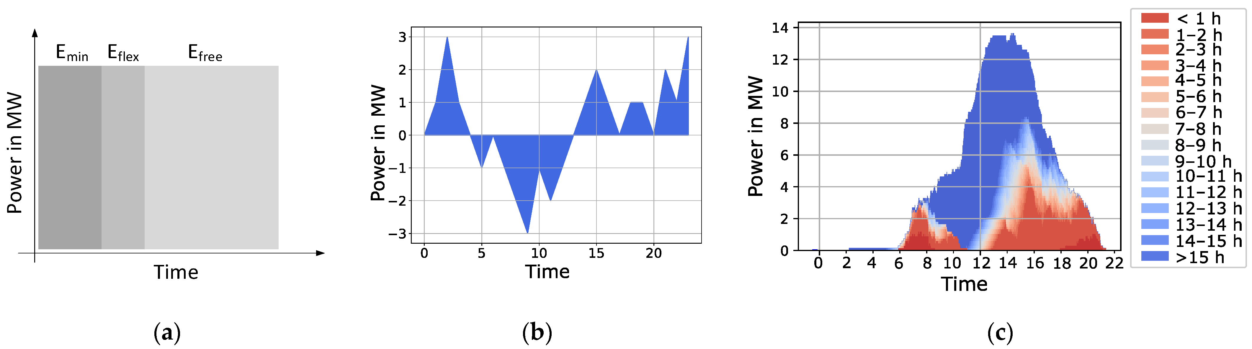
• The base load is added to the flexibility calculation. The base load consists of two types of loads. One is the buses that arrive at the bus depot during the day, charge for a short period of time to reach the minimum SoC needed for the next trip, and then take the next planned trip immediately. The charging of these buses has no shifting potential and is therefore considered as a base load. Another type of base load is electrical preconditioning. The preconditioning cannot be shifted for any of the buses at the depot since they always need to be preconditioned before departure.
• Flexibility is presented for a fixed amount of time into the future and in time categories based on time blocks of 15 min. This compressed way of flexibility quantification brings benefits regarding flexibility communication, data exchange, and the eventual application of optimization methods. Both the amount of time in the future as well as the time blocks can be adjusted depending on the needs of the flexibility provider and aggregator, or the requirements of specific markets where the flexibility is used.
• In order to incorporate the aspect of time in the best possible manner, meaning the duration of the flexibility, the visualization approach presented in [26], in Figure 6c, is used and extended by adding the base load.

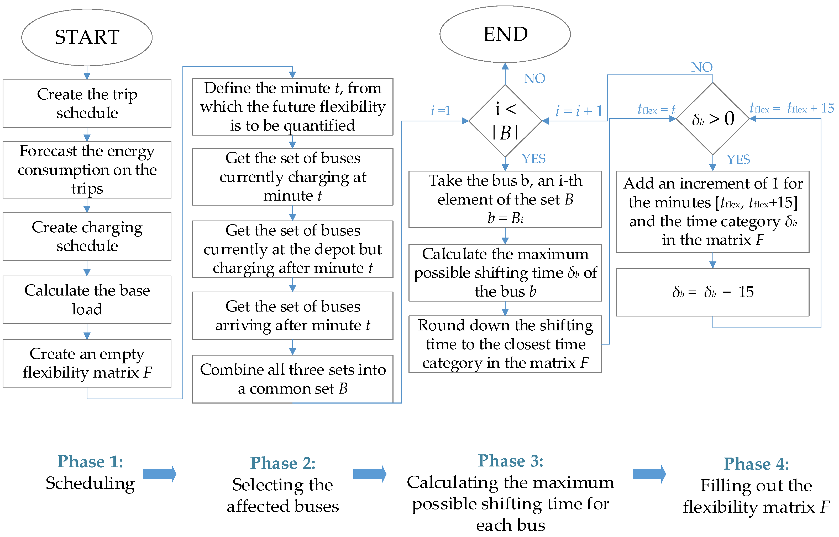
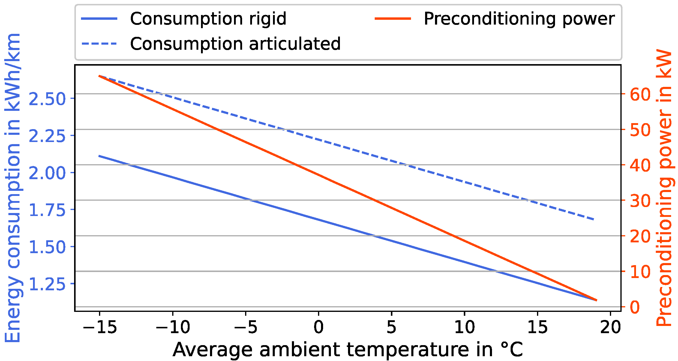
The block diagram in the Figure 7 shows the process of the flexibility quantification in this paper. The process follows four distinguished phases. In the first phase, the trip and charging schedule are created for a chosen period of time. The basis for the creation of these schedules is the forecast of the expected energy consumption during the trips, based on the average energy consumption shown in Figure 3. In this phase, an empty flexibility matrix F is also created in a form defined in Equation (6):

$$F=\left[\begin{array}{ccc}{F}_{t, cat0}& \cdots & F_{t,catn}\\ ⋮& \ddots & ⋮\\ F_{t+m,cat0}& \cdots & F_{t+m,catn}\end{array}\right]$$

(6)

The rows of the matrix represent the flexibility for different minutes, starting with a chosen initial minute t and ending after m minutes, with an increment of one minute. The columns of the matrix represent flexibility in different time categories, starting with the category “cat0” and ending with an n-th category “catn”. The categories in this paper are defined in 15 min time blocks, inspired by the flexibility calculation in [29]. A total period of 4 h is observed. The first category “cat0” represents the loads with shifting potential from 0 to 15 min. On the other hand, the last category “cat240” represents the loads with shifting potential of more than 240 min. For example, the flexibility $F_{1,225}$, per this definition, represents the total amount of load in the first analyzed minute that has a time flexibility of at least 225 min. However, the proposed method can be implemented with any other time categories as well. In the second phase, the foundation for further flexibility calculation is set. First a minute t is chosen, representing the time from which flexibility is going to be calculated. After choosing t, the set of buses B is defined, containing the buses that are currently charging at minute t, buses that are going to charge after the minute t, and the buses that are arriving after the minute t. The buses in the set B are the ones that are relevant for further flexibility calculations. In phase 3, each of these buses is looked at individually. For each bus, b the maximum possible shifting time and δ_b is defined. The shifting time δ_b represents the amount of time that is available after the end of charging and until the next planned departure, as defined in Equation (7):

$${\delta }_b=d_b-a_b-l_b$$

(7)

The shifting time is rounded down to the nearest available time category defined in the flexibility matrix F. In the fourth and final phase, the flexibility matrix is filled from the minute t until the last possible minute to which the load can be shifted. Hereby, for each minute, the appropriate time category is chosen defining how long into the future the load can be shifted.

4. Flexibility Quantification for the Analyzed Bus Depots

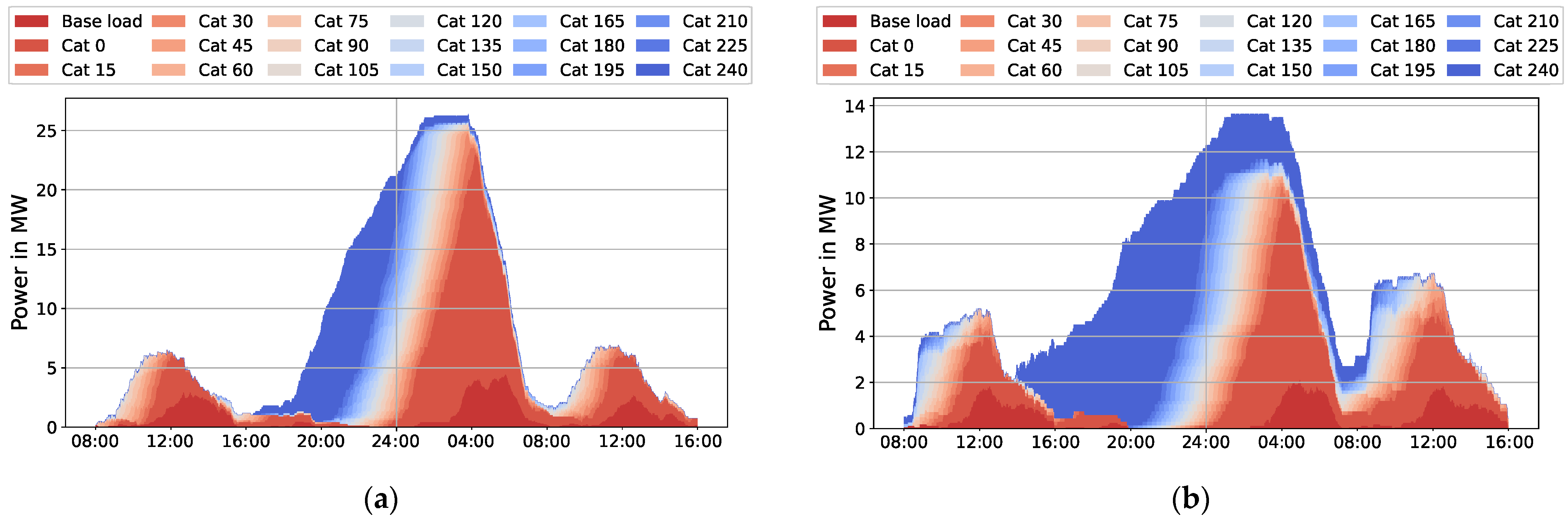
Figure 8 shows the calculated flexibility for the two analyzed depots, calculated at 08:00 h for a period of 36 h in advance for a typical working day. As it can be seen, the BD1 can reach a theoretical maximum possible power of 26.3 MW, whereas BD2 can reach 13.6 MW. Both of the depots reach this maximum possible power in the period from 02:00 h to 04:00 h. Regarding the duration of the flexibility, both of the depots show the biggest potential in the period from 16:00 h to 24:00 h. In this period, the majority of the load is in the category “cat240”, meaning that it can be shifted for 4 h or more in the future. The least flexible load is also similar for both of the depots, which is the load in the period from 08:00 h to 16:00 h, as well as the period in the early morning hours from 02:00 h to 08:00 h. This behavior is expected. In the period from 08:00 h to 16:00 h, the vast majority of the buses is on a trip and not at the depot. The buses that do come back to the depot during this period do not stay long, since the majority of them have their next scheduled departures on the same day. The lack of flexibility in the early morning hours from 02:00 h to 08:00 h can be explained by the fact that the buses need to depart soon. Additionally, in this period there is a significant preconditioning load representing a base load that cannot be shifted.

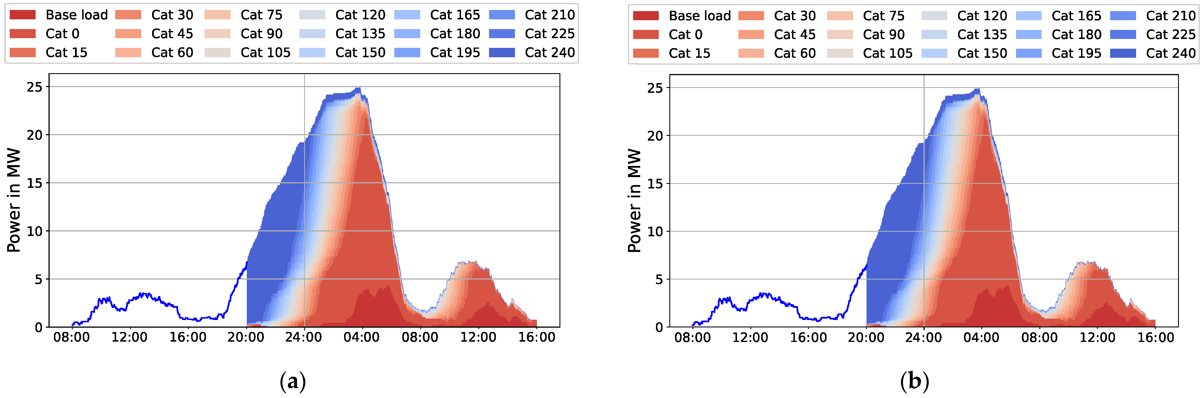
The flexibility shown in Figure 8 is observed for the next 36 h and from the perspective at 08:00 h. However, as the day progresses, the flexibility is going to change. This is because the buses are going to charge. Depending on the chosen charging concepts, they charge either directly upon their arrival at the depot or as scheduled for load peak minimization. As soon as they have finished with charging, they are no longer available for load shifting and cannot contribute to the flexibility provision. If the same period of 36 h (as shown in Figure 8) is observed, but at a later standpoint, the available flexibility decreases. 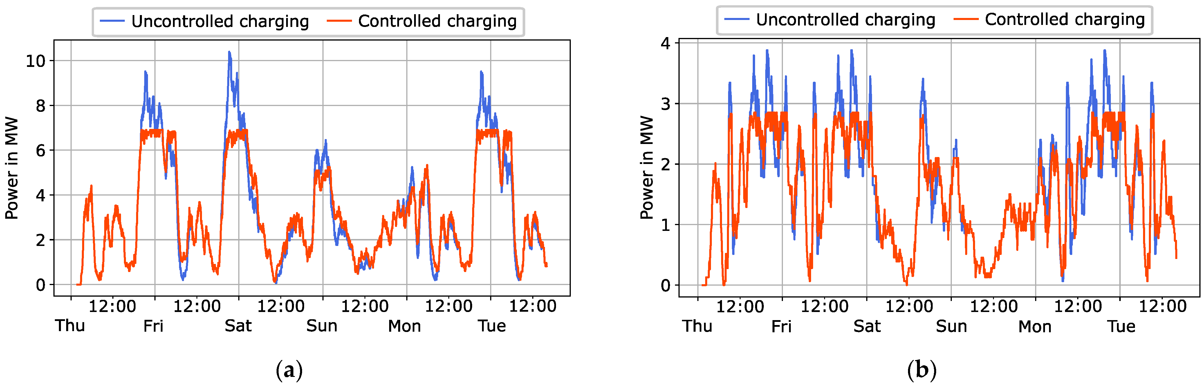This is shown in Figure 9, for flexibility calculated at 20:00 h and 24:00 h, as well as 04:00 h and 08:00 h on the following day, respectively. The figure shows flexibility for both controlled and uncontrolled charging. At 20:00 h (Figure 9a), the majority of the load can be shifted for more than 4 h. If all of the charging events are postponed until the latest possible point, the diagram shows approximately 23 MW of load peak at 04:00 h that cannot be further shifted or has a flexibility of less than 15 min. At 24:00 h (Figure 9c), the situation has changed. Since a large portion of buses has already fully charged, or at least started charging, the potential for load shifting is lower. If all of the remaining charging events at this point would be postponed until a further feasible time, there would be approximately 10.4 MW of load peak at 04:00 h that cannot be further shifted or has a flexibility less than 15 min. At 04:00 h and 08:00 h (Figure 9e,g), there is only a limited amount of flexibility left because the majority of the buses has already charged.

With uncontrolled charging there is only negative flexibility. This means that when necessary, the load can be reduced. This is because all of the buses charge immediately upon their arrival at the depot. Since none of the buses postpone their charging in advance, there is no possibility to add load afterwards. With controlled charging on the other hand, it is possible to achieve both positive and negative flexibility at certain time slots. In this case, the buses charge according to the schedule, which is not necessarily immediately upon their arrival. This means that the buses can start charging at a later point if the positive flexibility is necessary. This is visible in Figure 9. At 20:00 h, there is no difference between controlled and uncontrolled charging, as Figure 9a,b show. This is due to the fact that even with the controlled charging (Figure 9b), all of the buses charge immediately upon their arrival. At 24:00 h, however, there is an obvious difference between controlled and uncontrolled charging. As shown in Figure 9d, with controlled charging, there is a possibility to not only reduce the currently available load (negative flexibility), but also to increase it (positive flexibility). Because the charging of some buses is scheduled for a later time slot, the total available flexibility is bigger compared to uncontrolled charging. If the maximum possible load at 04:00 h is observed, Figure 9d shows 2 MW more than Figure 9c. 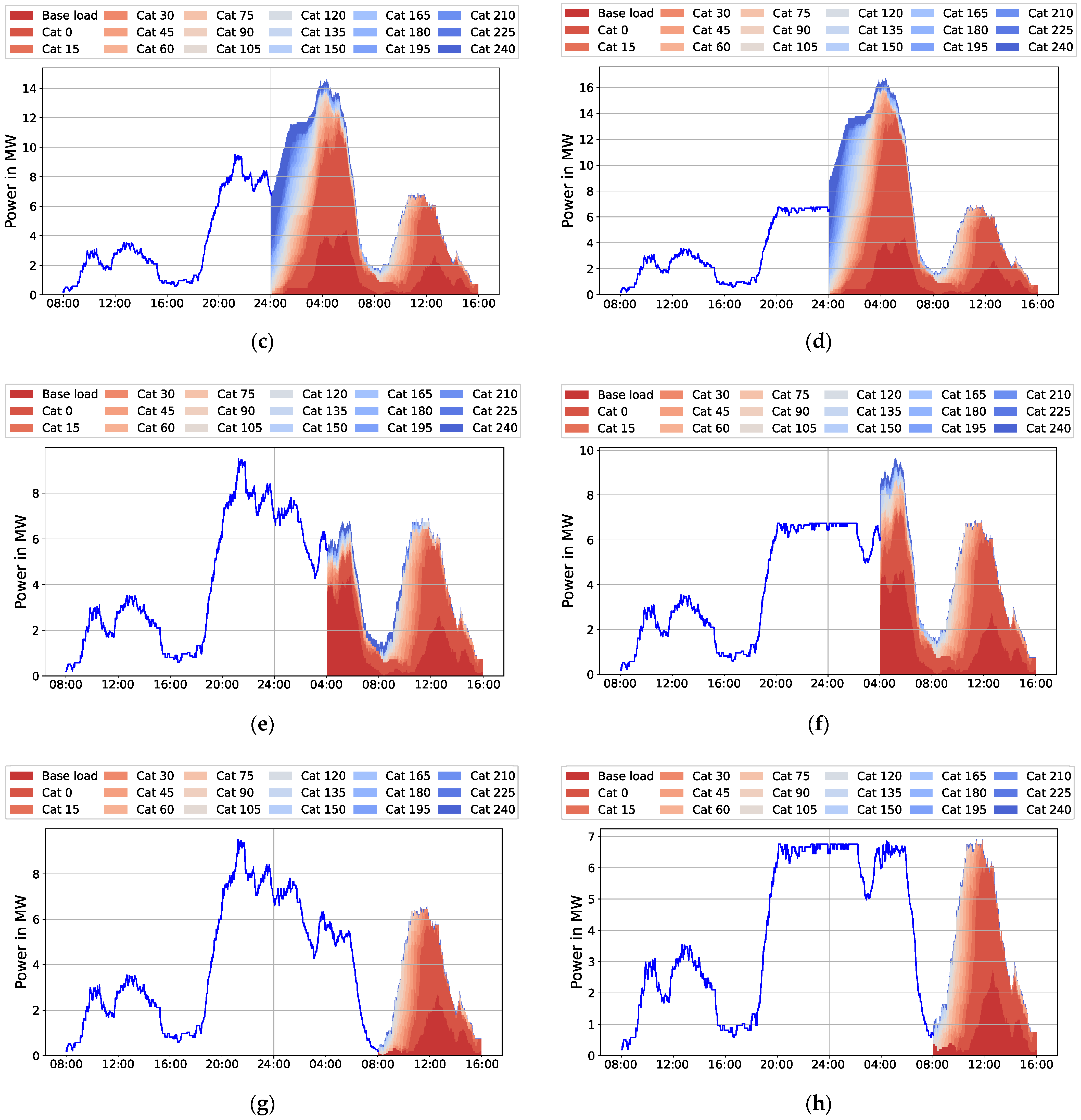Figure 9e,f show the flexibility with controlled and uncontrolled charging from the perspective of 04:00 h, as well as Figure 9g,h, which showing the flexibility from the perspective of 08:00 h, demonstrate similar behavior. The change in flexibility for different observed hours at the BD2 shows similar behavior to BD1, as shown in the Appendix A in the Figure A1.

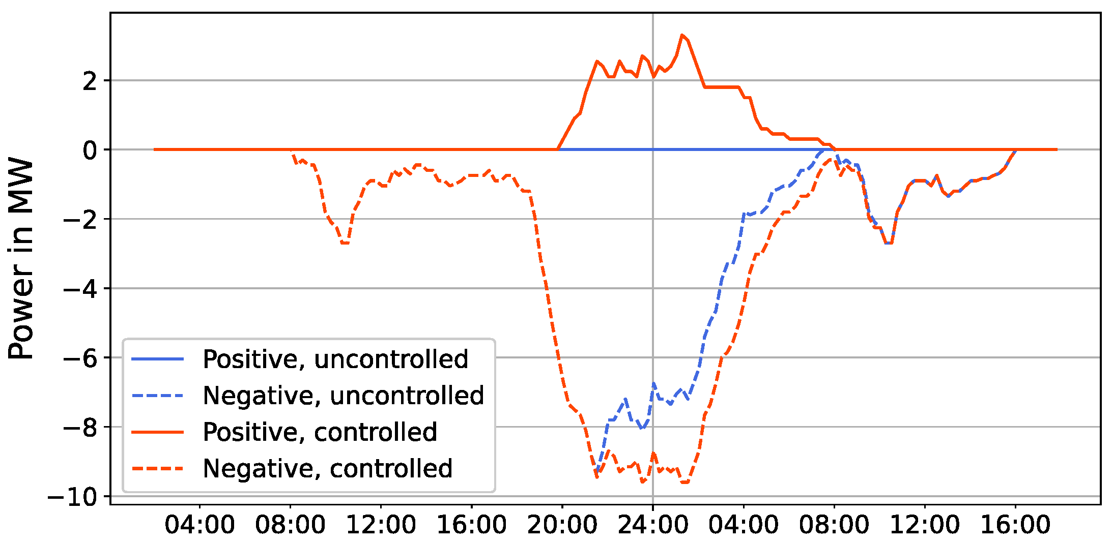
In order to emphasize the difference between uncontrolled and controlled charging, Figure 10 shows instant power flexibility for the BD1 for the period of 36 h. It is the same time range as shown previously in Figure 9. However, this time, only currently available power flexibility in the minute t is shown, without its duration. The positive instant flexibility is calculated as the difference between the current load at the minute t and the maximum possible load in the same minute. On the other hand, the negative instant flexibility shows the difference between the current load at the minute t and the base load in the same minute. As it can be seen, both controlled and uncontrolled charging offer instant negative flexibility during the observed time range of 36 h. With the uncontrolled charging however, in the time range from 20:00 h to 08:00 h on the following day, there is less available negative flexibility. If the positive flexibility is observed, the difference between controlled and uncontrolled charging is more significant, whereas the uncontrolled charging provides no positive flexibility at all. Furthermore, with the controlled charging, there is instant positive flexibility in the time range from 20:00 h to 08:00 h on the following day.

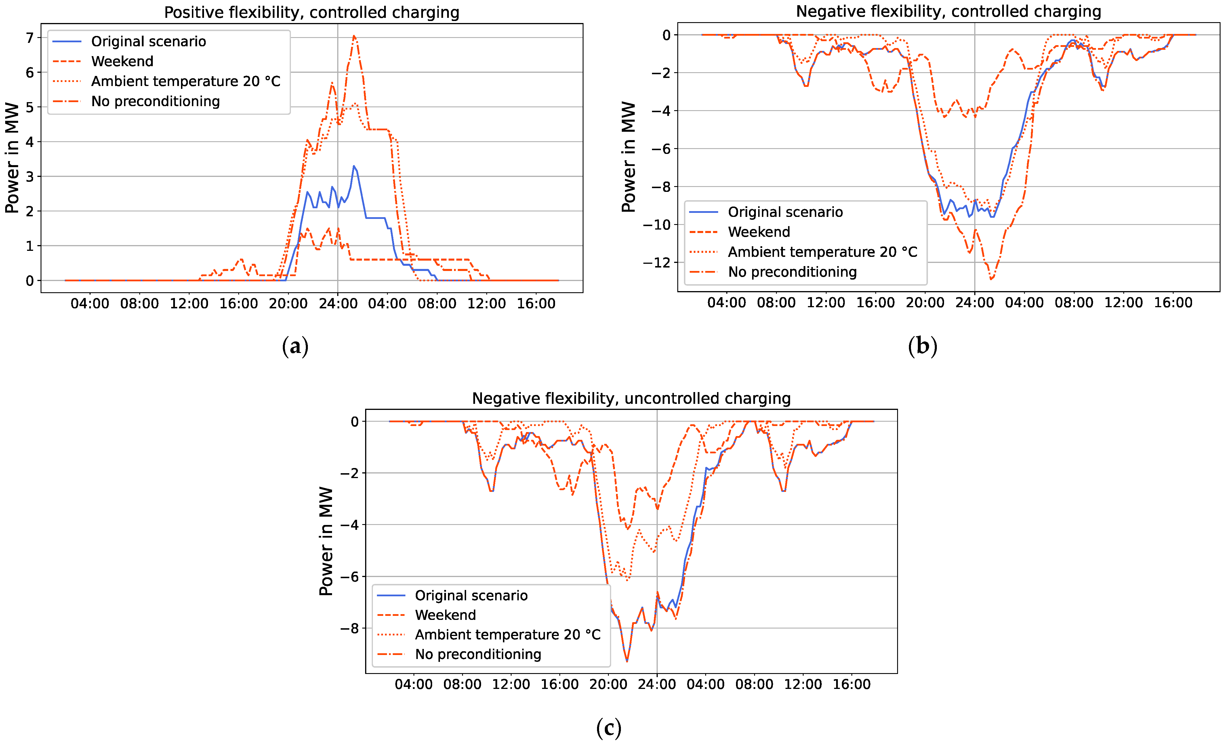
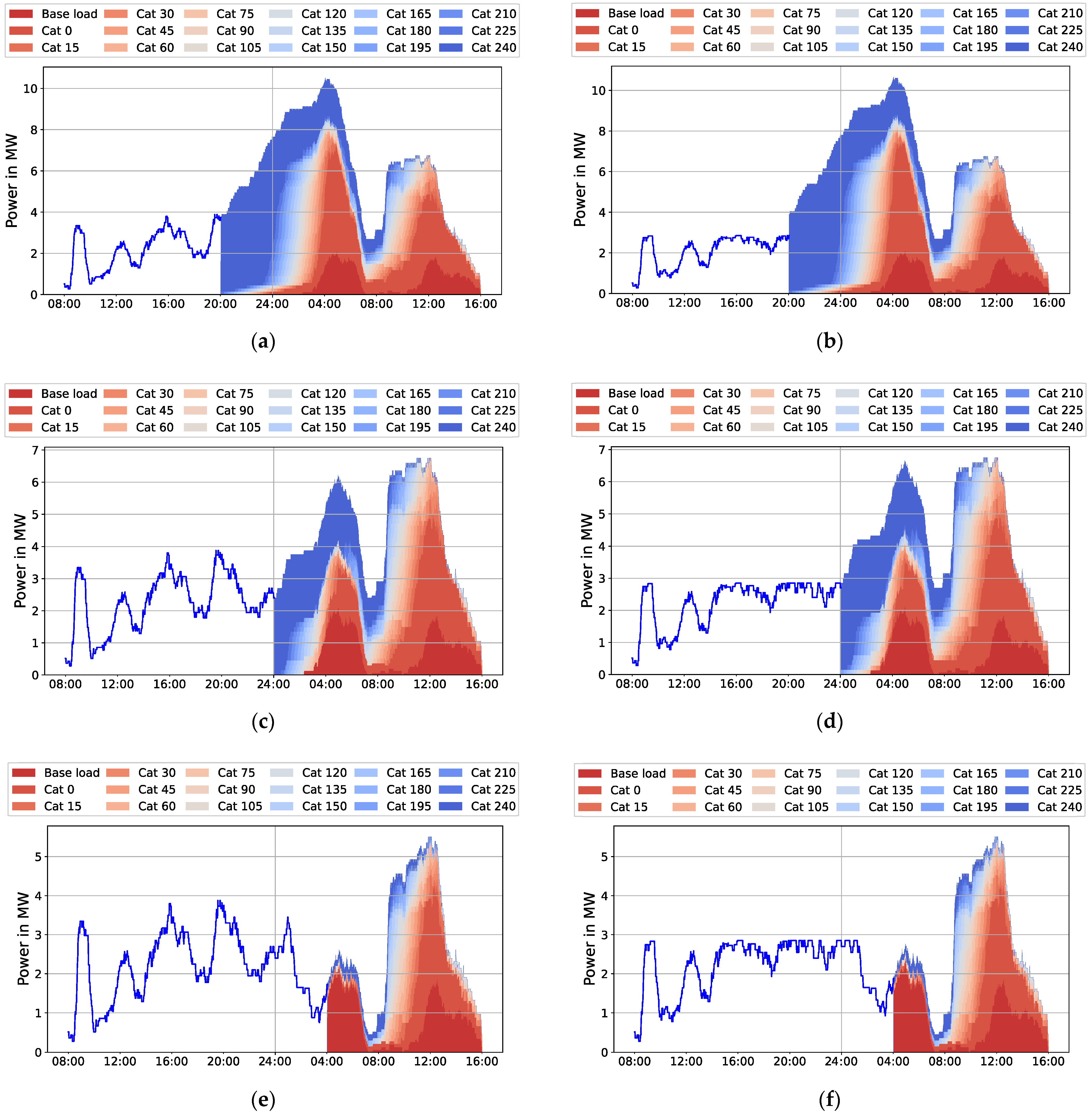
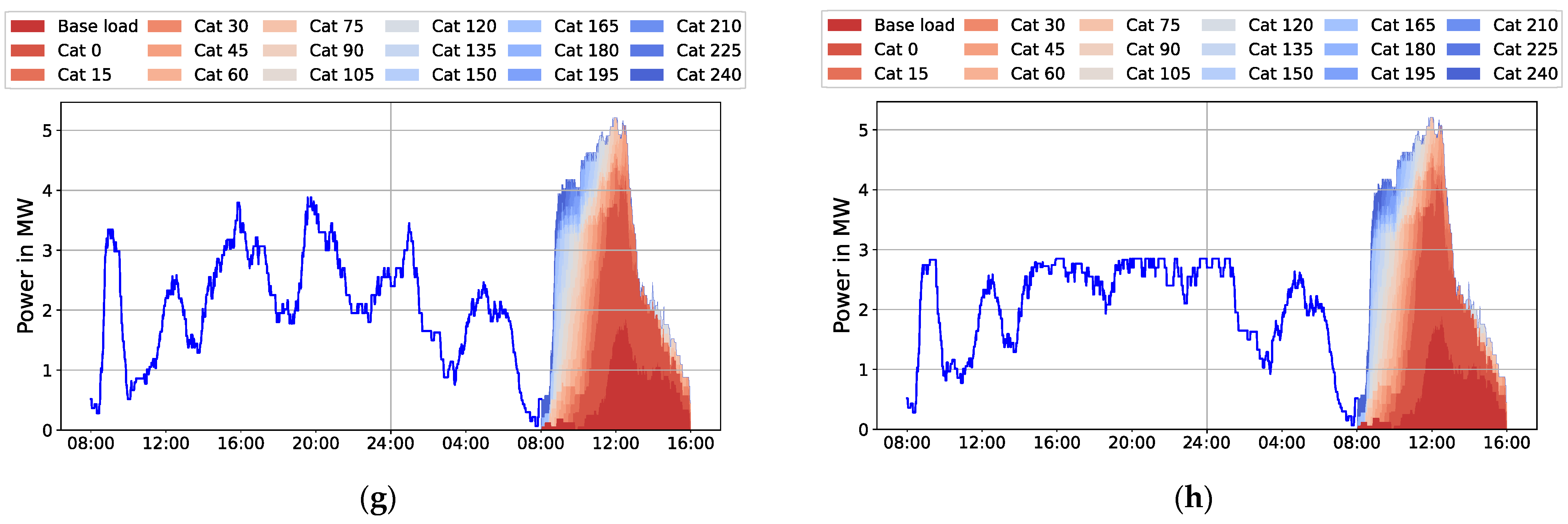
5. Sensitivity Analysis—Factors Affecting the Available Flexibility

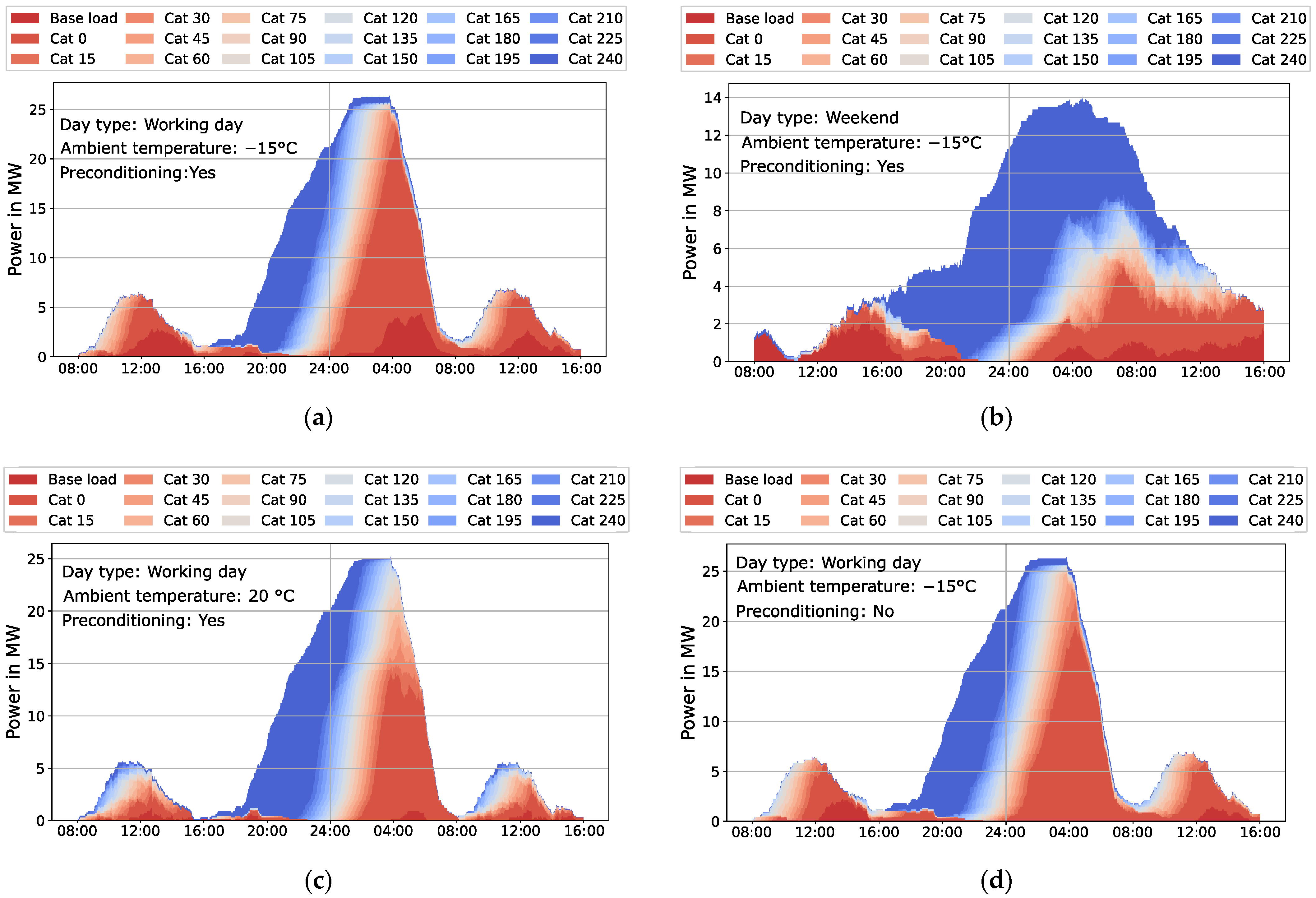
Multiple factors affect available flexibility on the bus depots. In this paper, three different factors are analyzed: the timeline (working day or weekend), ambient temperature, and electrical preconditioning, as shown in Figure 11. The impact of these parameters was analyzed based on the example of BD1. The original scenario demonstrates a working day, an ambient temperature of −15 °C, and electrical preconditioning of the buses, as shown in Figure 11a for comparison purposes. Figure 11b shows the flexibility on a weekend day. As it can be seen, there is a significant difference compared to a working day. The base load, as well as the load with flexibility smaller than 15 min (cat 0), is significantly smaller. On the other hand, there is more available load with flexibility over 4 h (cat 240). This behavior is expected. The load on the weekend is generally smaller since the buses have fewer trips to cover. Additionally, there is a significant number of buses with longer resting times at the depot during the weekend. The charging of these buses can generally be shifted for more than 4 h. This means that the flexibility potential on the weekends is higher than on the working days. Figure 11c shows the available flexibility for the case of an ambient temperature of 20 °C. Compared to the scenario shown in the Figure 11a, with a −15 °C ambient temperature, the buses in this case consume less energy and consequently need to charge less. Additionally, the preconditioning in this case occurs with a lower power. For this reason, the base load, as well as the load with flexibility under 15 min, is smaller compared to the original scenario at −15 °C. In addition, in this case there is more available load with flexibility over 4 h (cat 240), which can be observed throughout the whole analyzed time range of 36 h. This leads to a conclusion that more extreme weather conditions with higher energy consumption reduce flexibility potential. The last analyzed scenario, showing flexibility without electrical preconditioning, is demonstrated in Figure 11d. In this case, there is a smaller difference from the original scenario with preconditioning. The difference can be observed in the early morning hours between 04:00 and 08:00. In the case of electrical preconditioning, there is up to 4.5 MW base load during this time range, since the majority of the buses during these hours need to precondition before their scheduled trips. In the case without electrical preconditioning, this base load is not present.

Figure 11 shows a comparison for different analyzed scenarios for the flexibility power as well as its time duration. However, there is also a difference in the instantly available positive and negative flexibility between the analyzed scenarios, as shown in Figure 12. The instant positive flexibility in the case of controlled charging is shown in Figure 12a. Compared to the original scenario (working day, ambient temperature of −15 °C and electrical preconditioning), the cases with the ambient temperature of 20 °C and without preconditioning show a higher instant flexibility. On the other hand, the analyzed case with the weekend day indicates smaller flexibility. Figure 12b demonstrates negative instant flexibility in the case of controlled charging. In this case, the original and the case with an ambient temperature of 20 °C show similar behaviors. Higher flexibility occurs in the case without preconditioning, whereas on the weekend, a smaller flexibility can be observed once again. In the case of negative flexibility with the uncontrolled charging, as shown in Figure 12c, a different behavior can be observed. In this case, the original and the case without preconditioning have similar flexibility, whereas the case with the ambient temperature of 20 °C shows smaller flexibility. The smallest available instant flexibility is again the case with the weekend scenario.

It is important to emphasize the difference between the calculated flexibility power and time duration, as shown in Figure 11, and the instant available flexibility shown in Figure 12. The difference can be well-explained using the analyzed “weekend” scenario. In Figure 11b, with high flexibility on the weekend and a significant amount of load that can be shifted for more than 4 h, can be observed. This means that on the weekend, there is high potential for the optimal usage of flexibility, if this usage is planned in advance. If the usage of flexibility is not planned in advance, and the fleet operator rather uses the instant available flexibility, as shown in Figure 12, there is significantly smaller flexibility potential on the weekend compared to the working days. The loss of flexibility is due to the fact that without advanced planning, the buses charge as soon as scheduled and are no longer available for flexibility provision.

6. Potential for Flexibility Usage in the Case of Electric Bus Depots

There are several markets available for the commercial usage of the available flexibility on the electric bus depots. The usage can be generally split into two main categories, grid-oriented and market-oriented use cases. An example of grid-oriented use cases in Germany are the frequency response reserves market, interruptible load market, or different types of flexibility markets. On the other hand, the electricity markets, such as the European Energy Exchange (EEX) or the European Power Exchange (EPEX) represent pure market-oriented use cases. All these markets have different legal and technical prerequisites for their participants. The frequency response reserves market is split into three main parts: primary containment reserve (FCR), frequency restoration reserve with automatic activation (aFRR), and frequency restoration reserve with manual activation (mFRR or minute reserves). A minimum bid size of 1 MW is a requirement for the participants for all of the three mentioned products. For aFRR and mFRR however, a minimum of 1 MW is allowed only as an exception in the case when the provider submits only one bid per product time slice in a specific regulation zone [30]. If the available flexibility on the analyzed bus depots in this paper is observed, it is obvious that there are time ranges in which the load does not reach 1 MW. This is for example the time range between 08:00 and 11:00, when the majority of buses is outside of the depot on their scheduled trips. This means, that depending on the size, the bus depots alone do not necessarily fulfill the requirements for the participation in the frequency response market, since individual depots do not provide enough reserves. However, pooling of multiple depots or integrating the bus depots in virtual power plants resolves this issue. An example of bus depots integrated in a virtual power plant was demonstrated in [17]. The market for interruptible loads also has high participation requirements with the minimum necessary availability of 5 MW [31]. The participation of electric bus depots in this case is also possible only with pooling. The transmission system operator (TSO) primarily uses the frequency response reserves market and the interruptible loads market. In recent years, there have been several pilot projects in Germany initiating the so-called flexibility markets, which are used by the distribution system operators (DSO) [32,33]. The flexibility markets allow usage of flexibility in the local distribution grid. Electric bus depots can be easily integrated in such markets. A further possibility for the commercial usage of flexibility is trading at the electricity markets EEX or the EPEX. In this case, the flexibility of electric bus depots can be used for optimal purchases, as demonstrated in [12].

7. Summary and Future Work

This paper proposes a method for flexibility quantification for centralized electric bus depots with unidirectional charging. The proposed method focuses on quantifying not only the available power flexibility but also its duration. The analysis based on two real bus depots in the city of Hamburg, Germany, shows a great flexibility potential, especially during the night when the majority of buses is at the depot. Both of the depots show the biggest flexibility potential in the period from 16:00 h to 24:00 h. In this period, the majority of the load can be shifted for 4 h or more in the future. The least flexible load is also similar for both of the depots. The analysis shows a limited flexibility potential in the period from 08:00 h to 16:00 h, as well as from 02:00 h to 08:00 h. Two scenarios with different charging management concepts were analyzed, uncontrolled charging where the buses charge immediately upon their arrival back to the depot and controlled charging with the goal of load peak minimization. With uncontrolled charging, it was possible to provide only negative flexibility, whereas with controlled charging, it was possible to have both positive and negative flexibility. This shows that, depending on the charging management, even the bus fleets with unidirectional charging can provide both positive and negative flexibility.

A sensitivity analysis observing additional parameters such as the day type (working day or weekend), ambient temperature, or the electrical preconditioning showed a great impact on the available flexibility. On the weekends, the analysis showed more flexible loads with longer durations compared to working days. The ambient temperature also made a great impact on the flexibility. The analyzed scenario with the temperature of 20 °C showed greater flexibility compared to the extreme weather condition of −15 °C. On the other hand, the electrical preconditioning led to smaller flexibility, since the load necessary for the electrical preconditioning can generally not be shifted.

The paper additionally provided a short summary of markets in Germany available for the utilization of flexibility, with the focus on the technical requirements for participation. The analysis showed that the participation in the frequency response reserves market or the market for interruptible loads is possible only when pooling multiple depots. In the case of the two analyzed depots, the participation in flexibility or electricity markets, on the other hand, would be possible, even for single depots.

The proposed flexibility quantification method allows a first simple assessment of available flexibility on centralized bus depots with unidirectional charging and can therefore support decisions regarding design of the system, potential business cases, or potential impact on the electrical grid. However, for a successful usage of the flexibility, the proposed method needs to be further developed. On one side it is necessary to extend the method with a detailed battery and vehicle model. This will allow a more comprehensive forecasting of the energy consumption during the trips. Furthermore, depending on the chosen optimization goal or business case, it is necessary to develop an intelligent charging concept with the optimal charging schedule taking all the requirements and characteristics of the desired market into account. These points are a part of the future work. Additionally, in this paper, only the unidirectional charging on big, centralized bus depots was considered, as this is the current case on the analyzed depots in Hamburg. In the case of bidirectional charging, the quantification method needs to be further developed, which is also a part of the future work. In this case, the developed charging concepts need to take battery ageing into account, as an additional factor.