Acceleration Feature Extraction of Human Body Based on Wearable Devices

Abstract

Wearable devices used for human body monitoring has broad applications in smart home, sports, security and other fields. Wearable devices provide an extremely convenient way to collect a large amount of human motion data. In this paper, the human body acceleration feature extraction method based on wearable devices is studied. Firstly, Butterworth filter is used to filter the data. Then, in order to ensure the extracted feature value more accurately, it is necessary to remove the abnormal data in the source. This paper combines Kalman filter algorithm with a genetic algorithm and use the genetic algorithm to code the parameters of the Kalman filter algorithm. We use Standard Deviation (SD), Interval of Peaks (IoP) and Difference between Adjacent Peaks and Troughs (DAPT) to analyze seven kinds of acceleration. At last, SisFall data set, which is a globally available data set for study and experiments, is used for experiments to verify the effectiveness of our method. Based on simulation results, we can conclude that our method can distinguish different activity clearly.

1. Introduction

In recent years, wearable devices provide great convenience for the collection of human body acceleration data. With the rapid development of pervasive computing, the research of human activity recognition and behavior monitoring have attracted more and more attention [1,2]. The study of human behavior monitoring mainly includes behavior perception, data collection, behavior modeling and behavior analysis [3,4,5,6]. Currently, there are two main forms of human body monitoring:

(1)

Video based body monitoring. The behavior monitoring method based on video images is used to recognize human activities by observing the image sequence taken by the camera [7,8,9]. However, visual tools such as cameras are usually fixed and are more suitable for indoor use. There are many limitations to the use of video image-based behavior monitoring for behaviors that penetrate indoors and outdoors and in different locations. For example, it is difficult to deploy and can be easily blocked by objects. Its identification and data processing methods rely heavily on the external environment and are highly intrusive to the privacy of human activities. In addition, if a more accurate identification rate is required, the requirements for data sources are higher.

(2)

Sensor based body monitoring [10,11]. With the development of micromachines, sensors can sense more and more content with low costs. Wearable devices can be attached to the human body and move with people, thus providing continuous monitoring without interfering with the normal activities of the wearer. Considering this advantage, many researchers are more inclined to use sensors as human body data acquisition tools. Wearable devices are favored by users because of their compactness, lightness, and ability to continuously monitor human behavior data.

Wearable devices are portable devices that can be attached to the human body, which can monitor the acceleration, position, heart rate and other parameters. It does not affect the wearer’s daily activities but can provide human parameters in real time. Ling B. et al. [12] recognized 20 human behaviors with the recognition rate 84% under unsupervised condition. This is the first use of multiple sensors for behavior recognition research work. Priyanka et al. [13] build a remote heart disease monitoring system. When the relevant indicators are abnormal, the patients can be rescued in time. Chao et al. [14] used distributed sensor networks for human motion recognition and proposes a linear settlement method to process sensor network data. However, there are many sensors and large amount of data, so the real-time performance is not satisfactory. Maekawa T. and Cheng J. [15,16] used the accelerometer and gyroscope sensor of mobile phone to collect human motion data, analyzes the time domain and frequency domain of the original data, and extracts the relevant eigenvalues. Then the J48 decision-maker combined with Markov model is used to get the recognition results. The method can identify people going upstairs, downstairs, running, walking, static and other states. However, the algorithm can only recognize a certain state of a person in a period of time, it can’t count the number of actions.

Feature extraction methods have direct impacts on the recognition accuracy [17]. Human behavior recognition can be considered as the classification of time-varying data. The methods of human behavior recognition can be divided into three types [18]: template matching, statistical pattern recognition and semantic description. The method based on template matching is an early method of human behavior recognition. It is a good choice when there is not a large number of samples for training [19]. Dynamic time warping algorithm (DTW) [20] is a common technology in template matching method which is applied to gait recognition. Compared with the template matching algorithm, the recognition accuracy of statistical pattern recognition method is higher. Statistical pattern recognition method is usually used for human behavior recognition based on acceleration sensor [21]. The commonly used statistical recognition methods include decision tree, k-nearest neighbor, Bayes, SVM, neural network and hidden Markov model (HMM) [22,23].

With the developments of behavior recognition technology, classification technology also develops, and different classification technologies correspond to different recognition performance. Foody G. M. et al. [24] adopts decision tree classification algorithm. The algorithm is suitable for processing non- numerical data, but not good at continuous data type. Moreover, the self-learning ability of the algorithm is poor [25], so it needs to customize different logic rules for each people, and the amount of calculation is also relatively large. When the number of recognition types increases, the rules will be more complex, which greatly increases the error rate of model recognition [26,27,28].

Although the feature extraction method has achieved good results, there are still many problems to be solved: (1) Even if the human body is performing the same activity, the data collected by wearable devices change with different locations. Therefore, it is necessary to understand the influence of their location on the data collection, which is important for the human behavior recognition; (2) Feature extraction is critical to human behavior recognition, and the extraction of effective feature values is based on a lot of prior experience. So far, most of the feature value extraction is still done manually and subjectively by researchers, which has low efficiency and reliability; (3) The data collection, processing and other tasks require great energy consumption. At present, many algorithms are still based on multi-sensor. Therefore, it is necessary to study the acceleration feature extraction based on single sensor.

This paper mainly studies the method of extracting the characteristic value of human motion acceleration. By extracting the characteristic value of the acceleration signal collected by the sensor, the preliminary preparation for human behavior recognition is made. We combine the genetic algorithm with the Kalman filtering algorithm. By using the genetic algorithm to encode the parameters in the Kalman filter, we proposed KGA algorithm. Then, we define Standard Deviation (SD), Interval of Peaks (IoP) and Difference between Adjacent Peaks and Troughs (DAPT) to distinguishing the feature value of different motions.

The rest of the paper is organized as follows: Datasets and acceleration feature extraction method are proposed in Section 2. In Section 3, some experiments have been done to verify the analysis results. In Section 4, we make some conclusions.

2. Methods

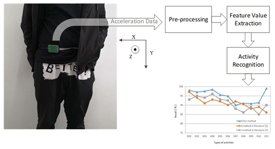
In the process of human behavior recognition, firstly, the original data of human body acceleration is obtained from the human body sensor, and then a series of processing is carried out on the original data to generate the behavior feature vector. The processing methods include filtering, smoothing, segmentation, data feature extraction, etc. Then the classifier is used to classify the behavior feature vector. Although the data processing methods of different recognition methods are different, their basic system framework is roughly the same from the macro perspective, and they are operated on the basis of sensor signal sequence.

2.1. Datasets

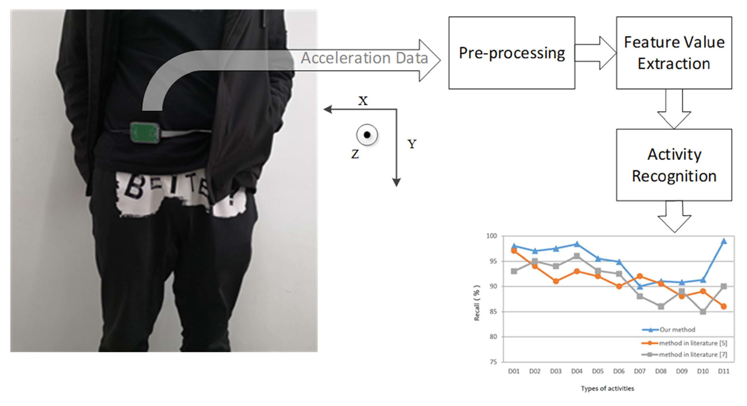
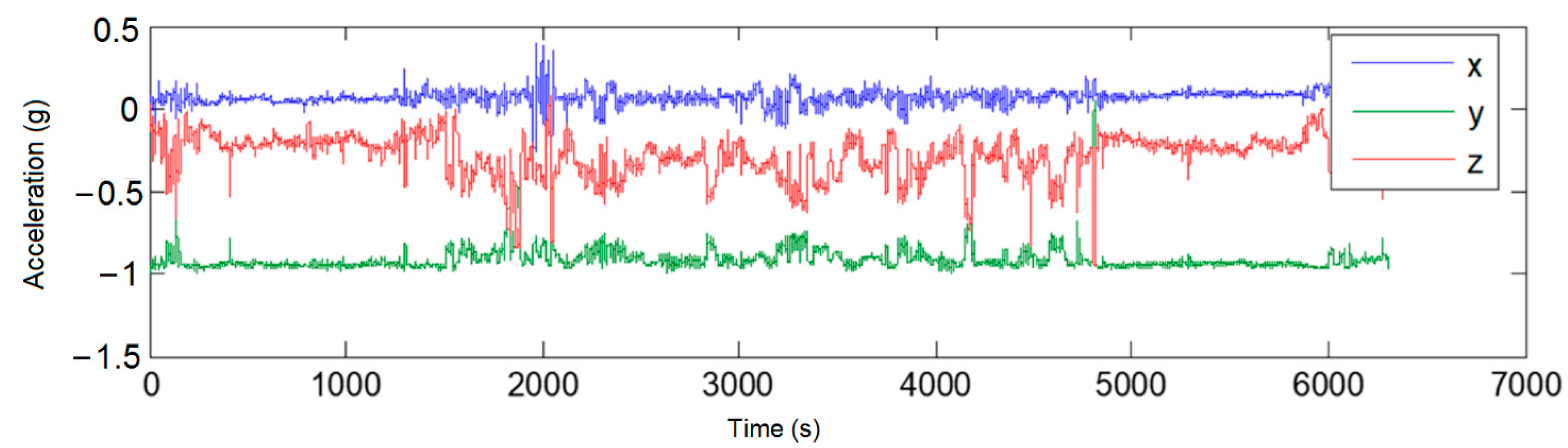
The difference of human body movements, number of sensor nodes and sensor placement produces different data sets. In order to facilitate the algorithm design and analysis, researchers have created some standard data sets for this issue. In this paper, we chose the globally available SisFall dataset for study and experiments. The SisFall dataset used a gyroscope and two acceleration sensors to obtain data from a sample of 4, 505 activities from 38 subjects. As shown in Figure 1, the wearable device is fixed at the waist of the tester, because the waist is easy to wear. The three-axis acceleration sensor can measure the acceleration in three directions, the front direction of the subject is the positive direction of X axis, the gravity direction is the positive direction of Y axis and the right side of the subject is the positive direction of Z axis. The data in SisFall are listed in

Table 1. Types of activities.

Number	Type	Number of Experiments	Duration (s)
D01	Walk slowly	1	100
D02	Walk quickly	1	100
D03	Run slowly	1	100
D04	Run quickly	1	100
D05	Go up and down the stairs slowly	5	25
D06	Go up and down the stairs quickly	5	25
D07	Sit→get up slowly in a half-high chair	5	12
D08	Sit→get up quickly in a half-high chair	5	12
D09	Sit→get up slowly in a low chair	5	12
D10	Sit→get up quickly in a low chair	5	12
D11	Jump up	5	12

[29].

2.2. Pre-Processing

The pre-processing of data is very important to the performance of the acceleration feature extraction method. The pre-processing must be simple and efficient. In order to remove the high frequency noise superimposed on the source data, we use the Butterworth filter to pre-processing the source data.

The system function $G\left(z\right)$ of the Butterworth filter can be calculated by Equation (1):

$$G\left(z\right)=\frac{{{\displaystyle \sum }}_{i=0}^M{b}_i{z}^{-i}}{1-{{\displaystyle \sum }}_{i=1}^N{a}_i{z}^{-i}}$$

(1)

The cut-off frequency is calculated by Equation (2):

$$\frac{F_p}{\sqrt[2N]{{10}^{0.1R_p}-1}}\le F_c\le \frac{F_p}{\sqrt[2N]{{10}^{0.1A_s}-1}}$$

(2)

where $R_p$ is the maximum allowable attenuation of the passband, $A_s$ is the minimum attenuation required for the stopband, and $F_p$ is the value after the precorrection of the passband cutoff frequency.

Then, according to the value of the filter order, the normalized system function $Gan\left(s\right)$ is calculated in Equation (3):

$$Gan\left(s\right)=\frac{d_0}{1+a_{1}s+a_2{s}^2+\dots +s^N}=\frac{d_0}{\left(s-s_1\right)\left(s-s_2\right)\dots \left(s-s_N\right)}$$

(3)

When $\Omega =0$, let $\left|Gan\left(s\right)\right|=1$ to determine the value of $d_0$, and when $a_0=1$, let $d_0=a_0=1$.

At last, let $s=s/F_c$, and convert it into a system function $Ga\left(s\right)$ of a low pass filter:

$$Ga\left(s\right)=Gan\left(s=s/F_c\right)=\frac{1}{1+a_1\frac{s}{F_c}+a_2{\left(\frac{s}{F_c}\right)}^2+\dots +{\left(\frac{s}{F_c}\right)}^N}$$

(4)

The process of filtering with Butterworth filters is the process of solving Equation (5):

$${\displaystyle \sum }_{k=0}^N{a}_{k}y\left(n-k\right)={\displaystyle \sum }_{m=0}^M{b}_{m}x\left(n-m\right)$$

(5)

In Equation (5), $a_k$ and $b_m$ are the system array of numerator and denominator of system function $G\left(z\right)$, sequence $x\left(n\right)$ is the signal sequence before filtering, and sequence $y\left(n\right)$ is the signal sequence after filtering. When $a_0=1,x\left(n\right)$ and $y\left(n\right)$ have the same length. The above equation is simplified as Equation (6):

$$y\left(n\right)={\displaystyle \sum }_{m=0}^M{b}_{m}x\left(n-m\right)-{\displaystyle \sum }_{k=1}^N{a}_{k}x\left(n-k\right)$$

(6)

When $k<0$, $x\left(k\right)=0$, $y\left(k\right)=0$, the value of the sequence $y\left(n\right)$ can be obtained after iteration. Parameter settings of Butterworth filter is shown in

Table 2. Parameter settings of Butterworth filter.

Parameters	Values
Sampling frequency $(Hz)$	25
Cut-off frequency $(Hz)$	5
Order	4

[29,30].

2.3. KGA Algorithm

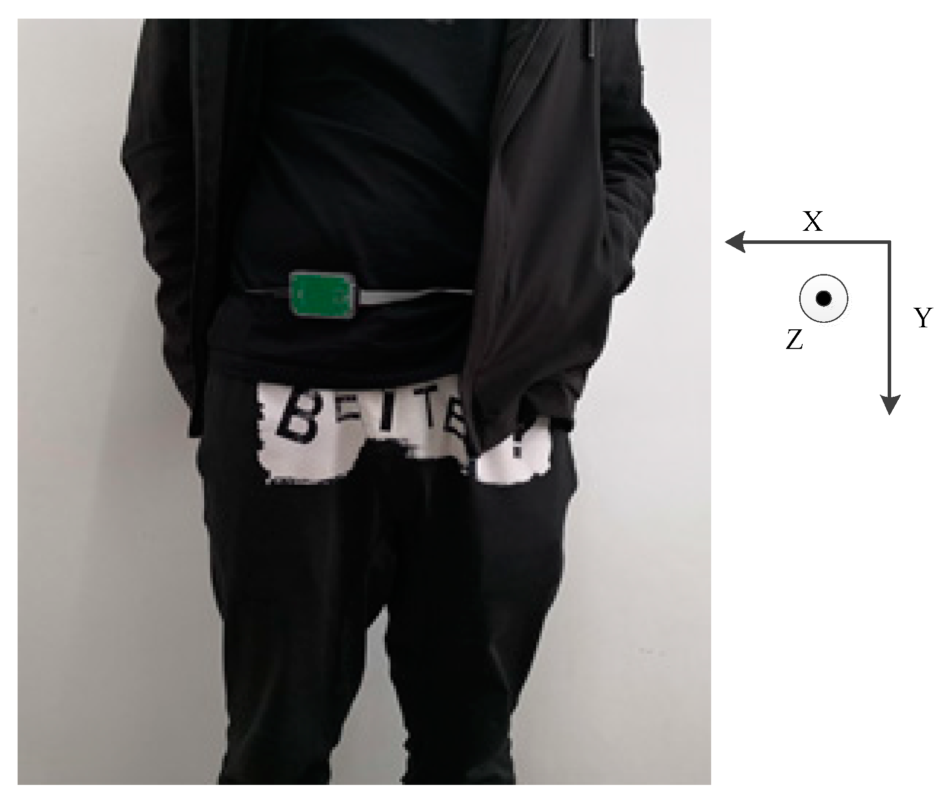
As the Butterworth filter cannot remove all noise points, to further smooth the source data, we combine the genetic algorithm with the Kalman filtering algorithm. By using the genetic algorithm to encode the parameters in the Kalman filter, we proposed KGA algorithm. This method consists of three steps: initialization stage, the optimization stage and the result output stage, and its flow is shown in Figure 2.

2.3.1. Initial Stage

In the initial operation of Kalman filtering algorithm, the parameters of Kalman filtering algorithm are generated in a random manner, which allows the subsequent genetic algorithm to encode the initial values. The calculation process of the Kalman filter algorithm [31] is as follows:

First of all, we introduce a linear stochastic differential equation, as shown in Equation (7):

$$Y(k)=MY(k-1)+NU(K)+\mathsf{\phi }(k)$$

(7)

where, $Y(k)$ is the system state at time $k$, $U(k)$ is the control quantity of system at $k$ time, $M,N$ is the system parameter value and $\mathsf{\phi }(k)$ represents process noise. The system measurement value $G(k)$ at $k$ time can be calculated by Equation (8):

$$G(k)=IY(k)+\mathsf{\theta }(k)$$

(8)

where, $I$ is the measurement system parameter, $\mathsf{\theta }(k)$ is the measurement noise. Let the covariance of $\mathsf{\phi }(k)$ and $\mathsf{\theta }(k)$ be $Q$ and $R$.

Suppose that the current system state is $k$, according to system model, the current system state can be predicted from the state of the system at the last moment, according to Equation (9),

$$Y(k|k-1)=MY(k-1|k-1)+NU(k)$$

(9)

where, $Y(k|k-1)$ is the predicted result using the previous state and $Y(k-1|k-1)$ is the optimal result of the previous state. $U(k)$ is the control quantity of the current state which can be set to zero if there is no control quantity.

The covariance $C$ corresponding to $Y(k|k-1)$ should also be updated after updating the system results, as shown in Equation (10):

$$C(k|k-1)=MC(k-1|k-1)M^{\prime }+Q$$

(10)

where, $C(k|k-1)$ is the covariance value of $Y(\mathrm{k}|k-1)$, accordingly, $C(k-1|k-1)$ is the covariance value of $Y(k-1|k-1)$ and $M^{\prime }$ is the transformation matrix of $M$.

Equations (9) and (10) are predicted values of the current system. The optimal estimates of the current state can be derived by combining the predicted values with the measured values of the current state:

$$Y(k|k)=Y(k|k-1)+Kg(k)(G(k)-IY(k|k-1))$$

(11)

where, $Kg\left(k\right)$ is the Kalman gain, as shown in Equation (12):

$$Kg(k)=C(k|k-1)I^{\prime }{[IC(k|k-1)I^{\prime }+R]}^{-1}$$

(12)

Finally, the covariance value needs to be updated so that the Kalman filter will keep running until the end of the system process. The updated equation is shown in Equation (13):

$$C(k|k-1)=[E-Kg(k)I]C(k|k-1)$$

(13)

where, $E$ is the unit matrix.

The prediction results of initial stage are taken as the input values of fitness function in the next stage.

2.3.2. Optimization Stage

In this stage, genetic algorithm is used to optimize each parameter of Kalman filtering algorithm, each individual in the population contains all the parameters of Kalman filtering algorithm. In this paper, the fitness value is represented by the difference between the source data and the output value of initial Kalman filter. The process of genetic algorithm [14] is as follows:

(a)

Selection operation. Select the best individuals from all the generated populations or generate new populations for inheritance, then evaluate them primarily by the fitness $F_i$ of each population. Make selection by method of roulette, so that the selection probability $P_i$ of each population individual can be expressed as:

$$P_i=\raisebox{1ex}{$F_i$}\!\left/ \!\raisebox{-1ex}{${\displaystyle \sum _{i=1}^N{F}_i}$}\right.$$

(14)

(b)

Crossover operation. Randomly select two population individuals for exchange and combination. Suppose the two populations are $x$ and $y$ respectively, and their crossing at $i$ position can be expressed as:

$$\{\begin{array}{l}{x}_i=x_i\ast rand()+y_i(1-rand())\\ x_i=y_i\ast rand()+x_i(1-rand())\end{array}$$

(15)

where, $rand()$ is a random number between 0 and 1.

(c)

Mutation operation. One individual population is selected randomly from all the generated populations for mutation operation. The variation of individual $x$ at $i$ position can be expressed as:

If rand() > 0.5

$$x_i=x_i+(x_i-x_{\max })\ast {(1-\raisebox{1ex}{$s$}\!\left/ \!\raisebox{-1ex}{$S$}\right.)}^2\ast rand()$$

(16)

If rand() = 0.5 or rand() < 0.5

$$x_i=x_i+(x_i-x_{\min })\ast {(1-\raisebox{1ex}{$s$}\!\left/ \!\raisebox{-1ex}{$S$}\right.)}^2\ast rand()$$

(17)

where, $x_{max}$ and $x_{min}$ represent the upper and lower bounds of an individual separately, s and S is the current hereditary algebra and the total hereditary algebra.

The genetic algorithm calculates the new fitness value after mutation operation. If the genetic algebra reached the setting values, the optimization result of Kalman filter can be got. Otherwise, the algorithm will continue the previous loop operation.

2.4. Feature Extraction

Feature extraction is very important in human behavior monitoring. Its goal is to extract parameters that can identify human behavior. Generally speaking, two methods have been proposed to extract features from time series data: statistical method and structural method. Statistical methods use quantitative features of data to extract features, while structural methods consider the relationship between data [29,30,32].

The feature values used in human behavior monitoring methods are extracted from accelerometers, gyroscopes, pressure sensors and so on, which are widely used in human behavior monitoring methods. However, it is still a problem that how to select the characteristic value to ensure the most convenient data processing and achieve the optimal recognition effect for the specific human activity to be monitored.

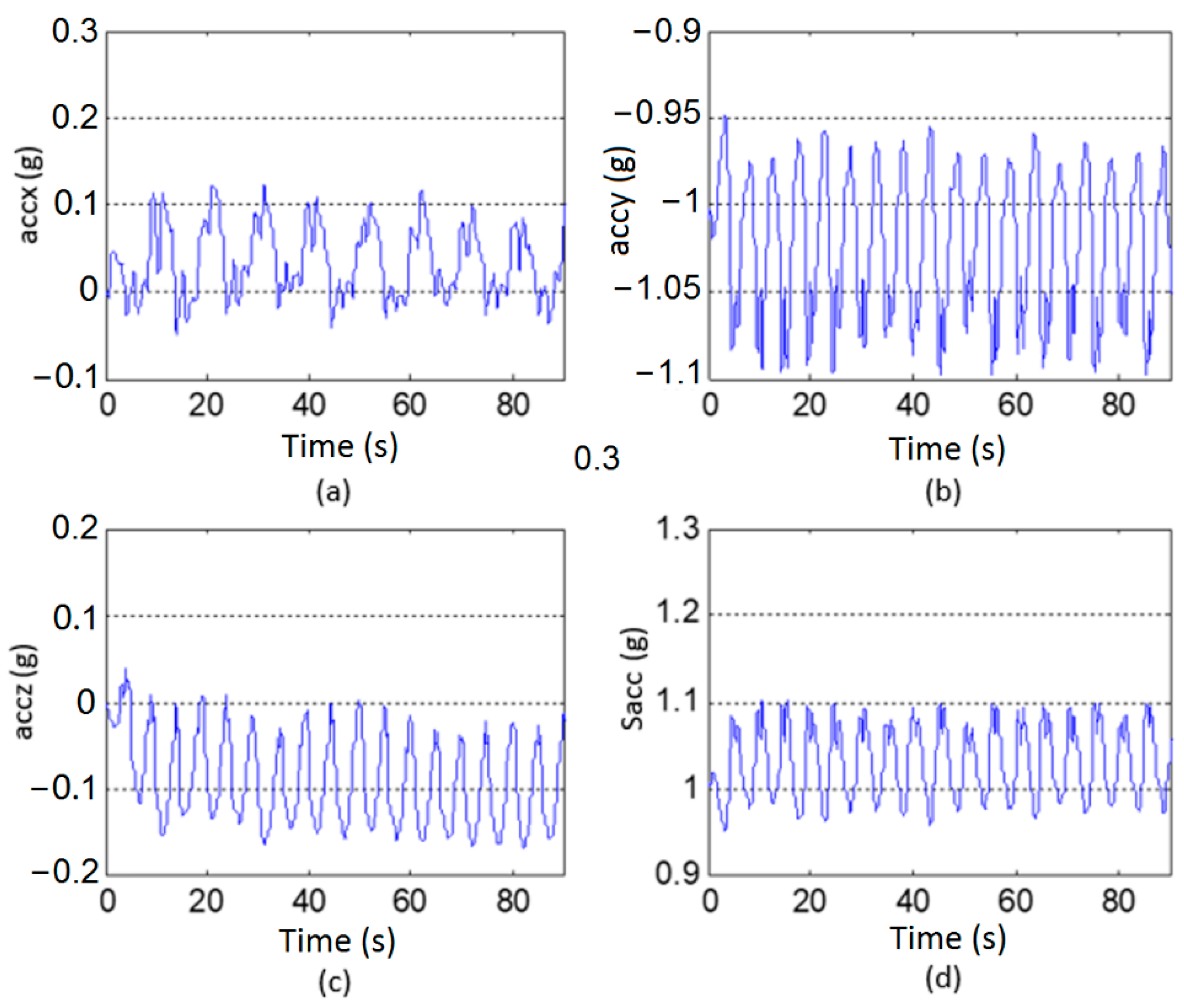
This paper only considers the acceleration changes of a certain action. First of all, the acceleration amplitude was used to describe different body motion. Since accelerations are vectors, their superposition value at a certain moment can be calculated by Equation (18):

$$Sacc=\sqrt{ac{c}_x^2+ac{c}_y^2+ac{c}_z^2}$$

(18)

where, $ac{c}_x,ac{c}_y,ac{c}_z$ represents the acceleration value in the $x$ axis, $y$ axis, and $z$ axis directions respectively. Taking D01 for example, as shown in Figure 3, the horizontal ordinate indicates time and the vertical ordinate indicates the acceleration value.

Other repetitive motion such as walking and running are all regular exercises. The graphical form of their acceleration data is similar to Figure 3. The difference lies in the intensity of exercise, stride size and stepping frequency. So, we propose Standard Deviation (SD), Interval of Peaks (IoP) and Difference between Adjacent Peaks and Troughs (DAPT) to distinguishing the feature value of different motions.

2.4.1. Standard Deviation

The degree of dispersion of the dataset can be expressed by the standard deviation. When human moves, the acceleration will increase accordingly, and the corresponding standard deviation will also have different values due to different types of motion. Therefore, using the standard deviation can clearly distinguish the static state of the human body from the motion state. We can calculate standard deviation by Equation (19):

$$SD=\sqrt{\frac{1}{N}{\displaystyle \sum }_{i=1}^N{(x_i-\mu )}^2}$$

(19)

Among them, $N$ is the number of data, and $\mu$ is the mean value of all the data.

2.4.2. Interval of Peaks

Since the human body’s stride frequency changes with different activities, such as going up and down stairs. Therefore, the interval between two adjacent peaks is used for distinguishing the kind of motion. As shown in Equation (20):

$$IoP=T_t-T_{t-k}$$

(20)

where, $T_{t-k}$ is the time when a certain wave peak appears, $T_t$ is the time when the next wave peak adjacent to the previous peak and $k$ is the number of sampling points of adjacent peaks.

2.4.3. Difference between Adjacent Peaks and Troughs

The amplitude of human body acceleration changes with different motions. The requirement of real-time is also very high. When extracting feature points, real-time requirements are very important. Therefore, this method will synthesize the extreme points of $Sacc$. So, we regard the peak and trough value as critical parameters. In the actual data processing process, when a new sampled value is received, it is compared with the previous one. If the turning point doesn’t appear, it continues to observe. If there appears a turning point, then this point is the extreme point. We consider the range between adjacent peaks and troughs of $Sac{c}_t$ as the extreme point, which can be calculated in Equation (21):

$$DAPT=Sac{c}_t-Sac{c}_{t-k}$$

(21)

Among them, $Sac{c}_t$ is the value of a certain wave peak or trough, $Sac{c}_{t-k}$ is the value of the adjacent wave trough and peak, and $k$ is the time between adjacent peak and trough.

3. Results and Discussion

3.1. Analysis of Filtering Algorithms

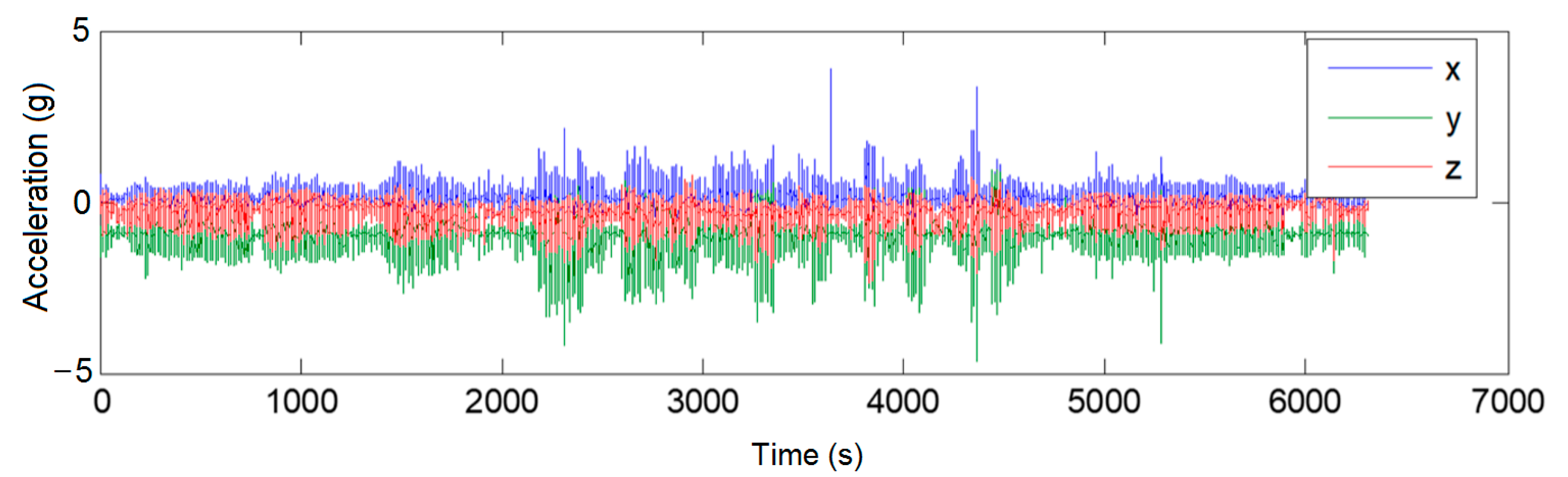
In order to verify the validity of KGA, we compared KGA with the Kalman filtering algorithm. These two methods are implemented on the SisFall dataset that shown in Figure 4. The source data range from −5 g to 5 g, and the fluctuation is very large.

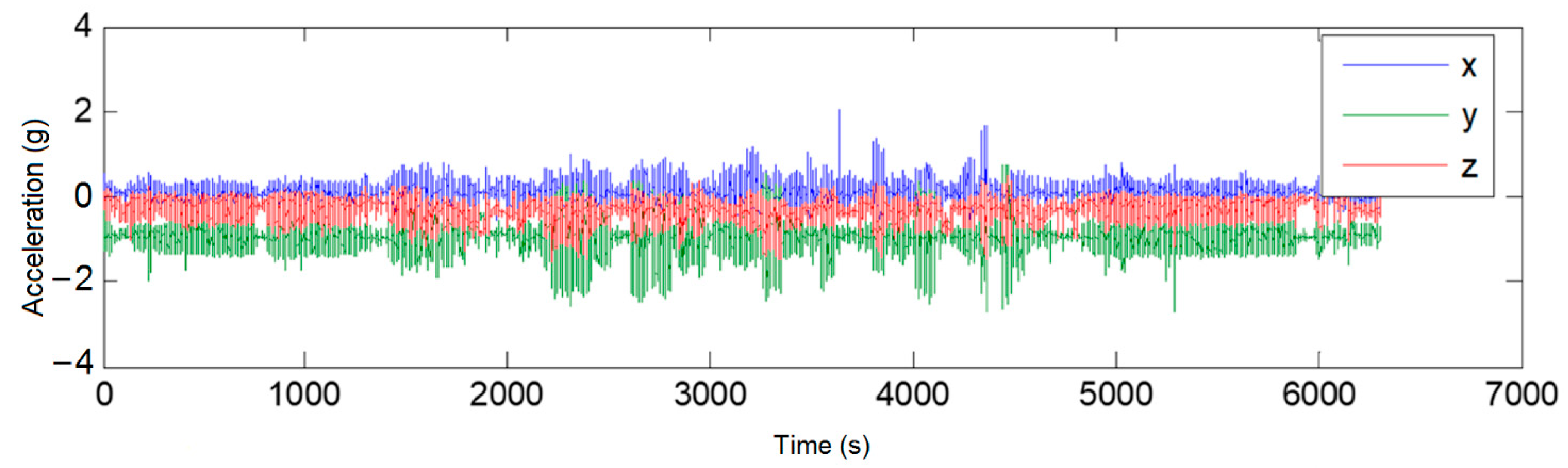
We first use Butterworth filter to deal with the data in Figure 3, and the result is shown in Figure 5.

As can be seen from the Figure 5, after the Butterworth filter, the high-frequency data has been removed and the low-pass filtered data become flat. The data range from −2 g to 2 g, and the data distribution is more concentrated.

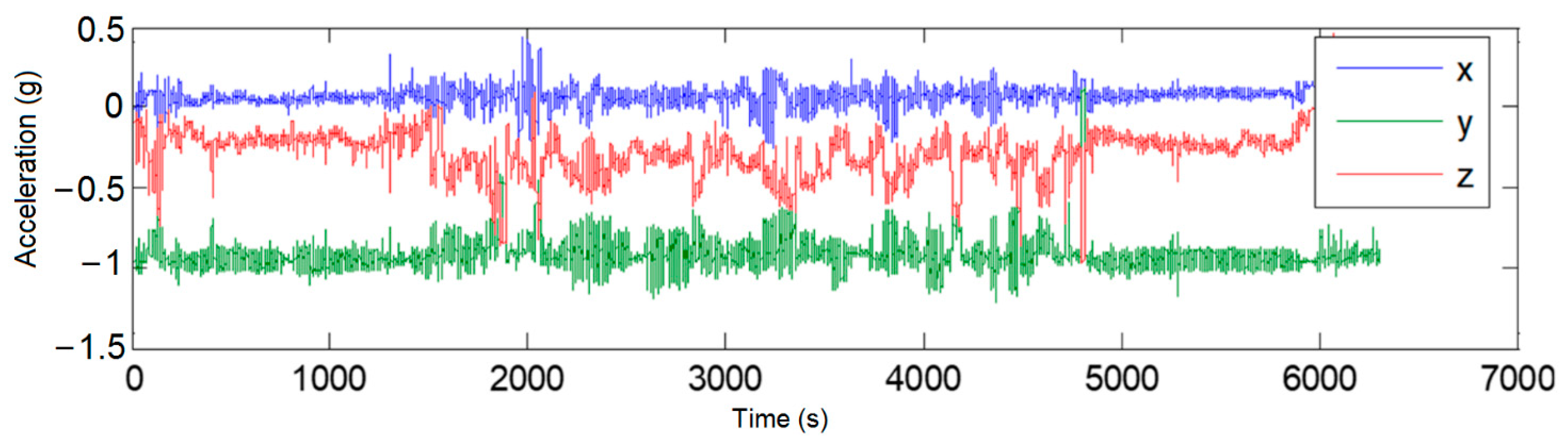
If the Kalman filtering algorithm is not optimized with genetic algorithm, the result of its operation is shown in Figure 6. While the result of the GA algorithm is decoded, and the optimal parameter value obtained is added to the Kalman filtering algorithm formula, the filtering result of this algorithm is shown in Figure 7.

As can be seen from the Figure 7, after the low-pass filtered data is processed again, the data range of the two is changed from [−2 g, 2 g] to [−1 g, 0.5 g], the data distribution is more compact, and the acceleration values in the three directions are more distinct. However, the data in Figure 6 fluctuates significantly more and contains more outliers, while the data in Figure 7 is smoother.

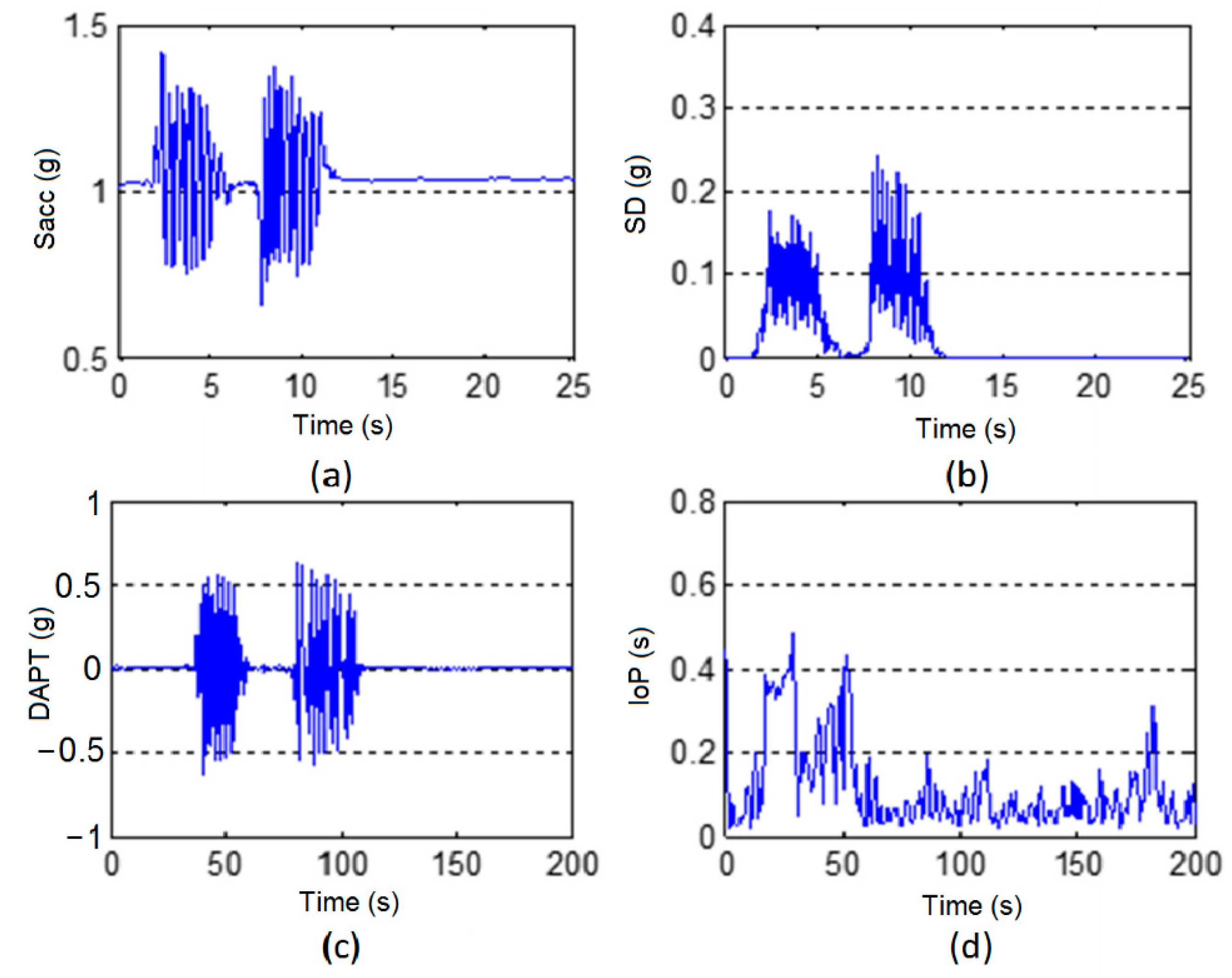
3.2. Analysis of Running Activity

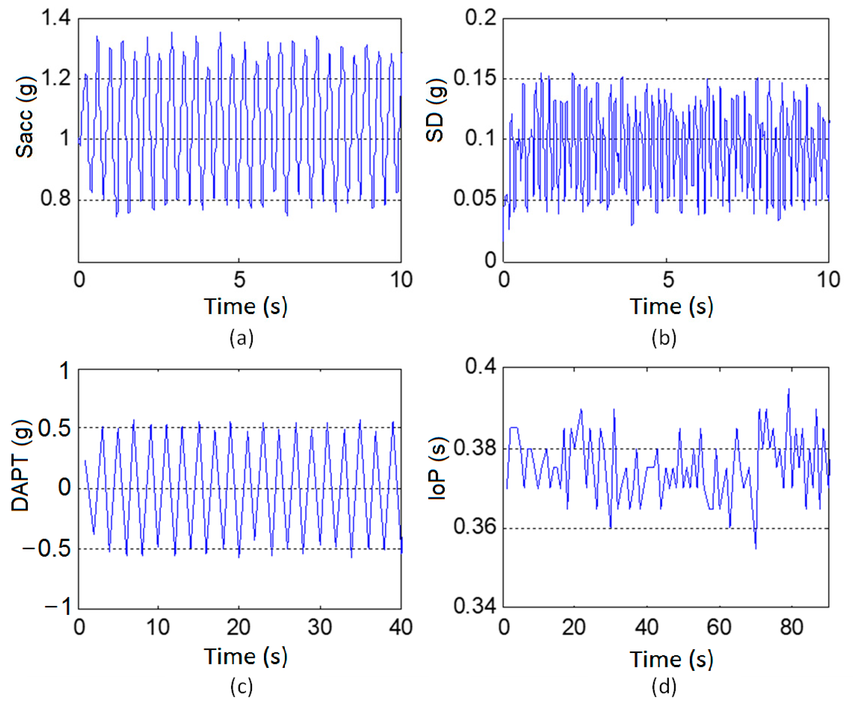
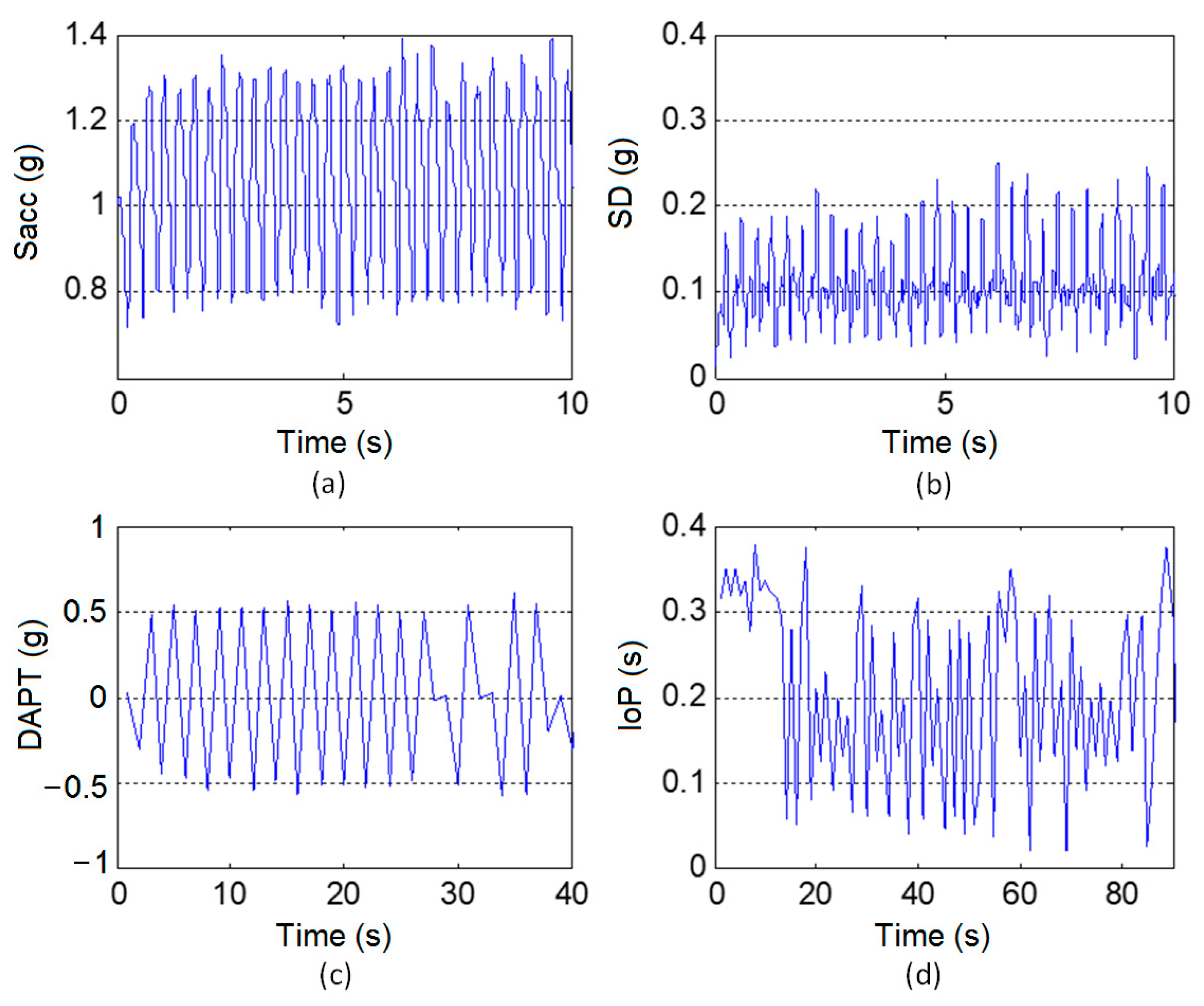
The simulation takes SisFall as dataset. Figure 8 and Figure 9 are the comparison of jogging and fast running. We randomly select an object from the data set and analyze its motion parameters. As can be seen in Figure 8 and Figure 9, the $Sacc$, $SD$, $DAPT$ waveforms produced by jogging and fast running are very similar. Since running is a cyclical exercise, the $Sacc$ of both of them have regular small peaks and the values are similar. Possible reasons are as follows: the difference between the speeds of jogging and fast running is not obvious enough; wearable device is not firmly worn. However, by analyzing the standard deviation of these two waveforms, it can be seen that the $SD$ produced by fast running is significantly greater than that produced by slow running. In addition, due to that human body runs faster than jogging, correspondingly, the stepping frequency of fast running is higher than that of jogging, the $IoP$ produced by fast running activities is less than that by jogging activities.

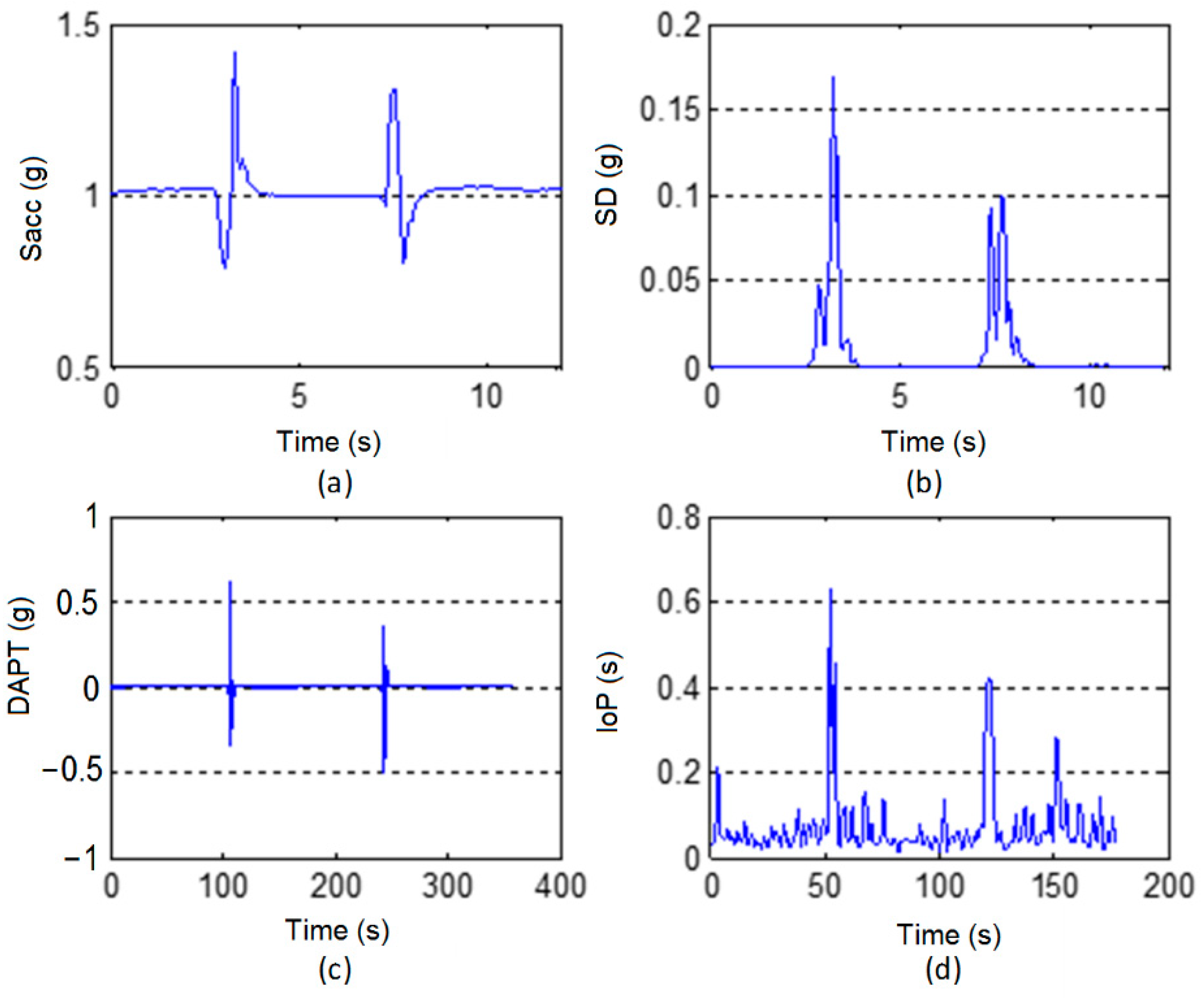
3.3. Analysis of Going up and down Stairs

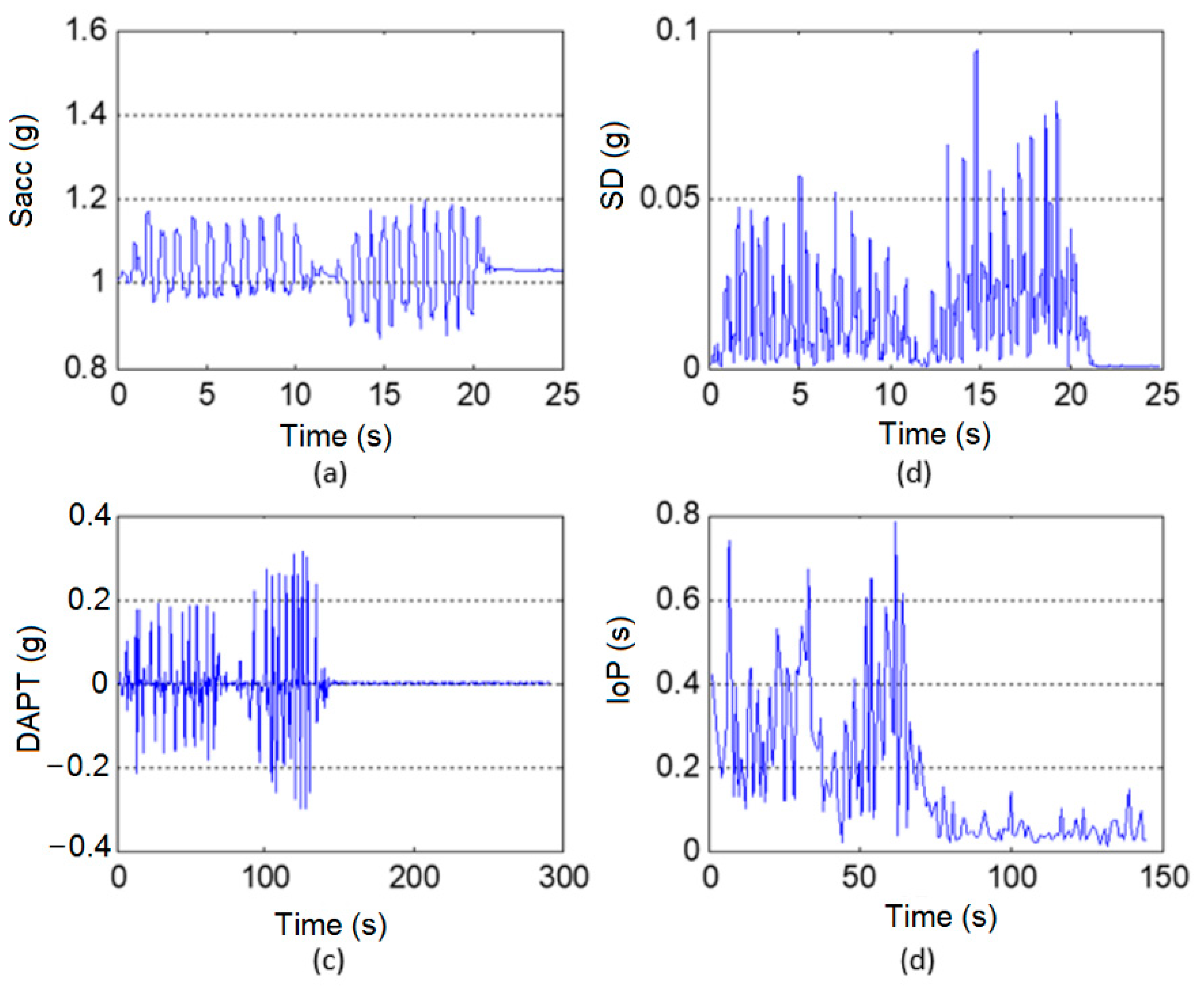
Going up and down the stairs is a repetitive motion. Figure 10 and Figure 11 are the comparison of slow up and down stairs and fast up and down stairs. By analyzing Figure 10 and Figure 11, the $Sacc$ generated by slow up and down stairs are significantly lower than that by the fast up and down stairs. It can be seen from the Figure 10 that the value of $SD$ generated by slowly going up and down stairs does not exceed 0.1 g, while the $SD$ generated by going up and down the stairs quickly is slightly larger, not exceeding 0.3 g. At the same time, the $DAPT$ of former is also smaller than that of latter. Similar to walking activities, since the human body is slower when going up and down stairs at a slow speed, correspondingly, the stepping frequency of this activity is lower, in terms of data, the $IoP$ is larger.

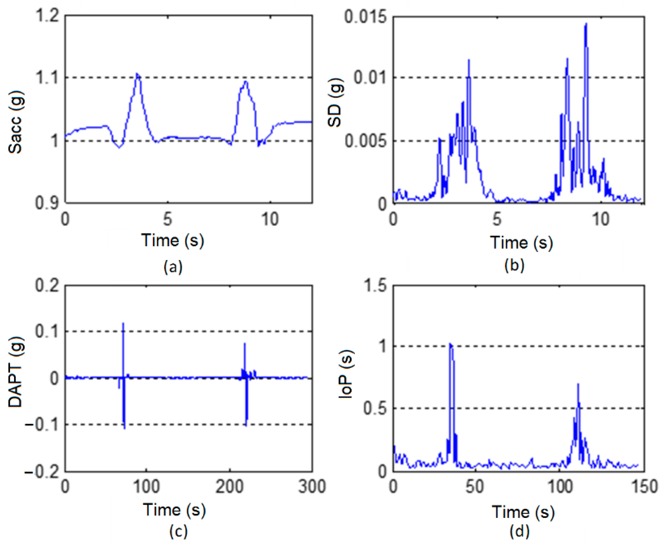
3.4. Analysis of Sit-Up Activity

This experiment takes D07 and D08 in Table 1 as examples to analyze the sit-up type activities, as shown in Figure 12. It can be seen from the Figure 13 that their $Sacc$ have large fluctuations, but due to the different speeds, the $Sacc$ of former has a smaller value. At the same time, there are two large fluctuations in the standard deviation of these two activities. Corresponding to the two movements of the human body, “sit down” and “get up”, since the slow activity is relatively stable. In terms of data, the $SD$ of former is much smaller than that of latter. The difference reached 10 times the order of magnitude. This is because when the human body quickly sits down and rises quickly from a half-height chair, the motion range is larger, the action is more violent, and the corresponding acceleration is greater, and $DAPT$ is also greater.

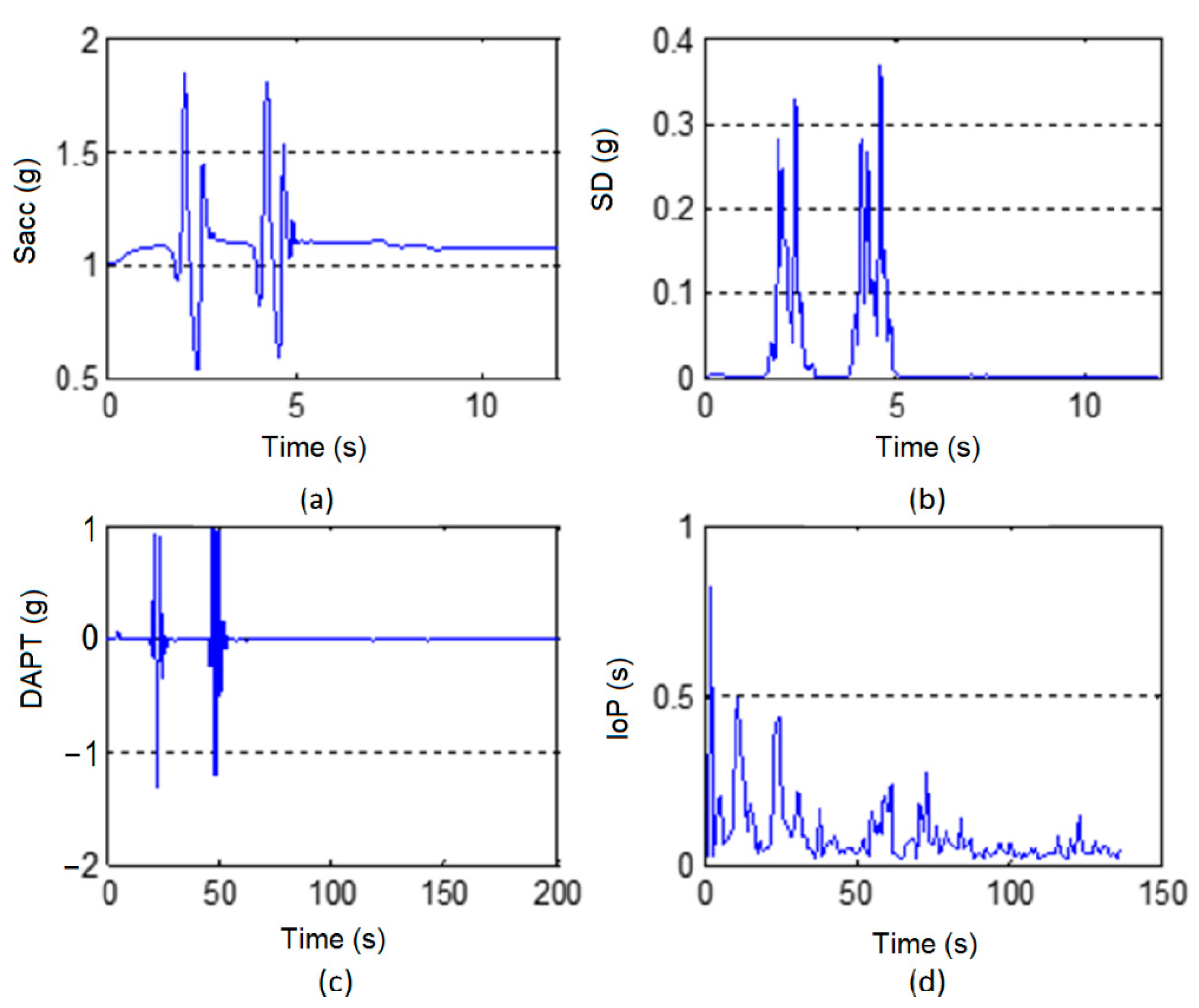
3.5. Analysis of Jumping Activity

Figure 14 is the analysis of jump movement. it can be found that the $Sacc$, $SD$, $IoP$ and $DAPT$ waveforms produced by the jumping motion are very similar to the sit-up motion. Both have large peaks and flat areas, especially the peak interval values are very similar. However, there are obvious differences in certain characteristics between the two actions of sit-up and jumping: although the two are both highly volatile activities, the $SD$ and $DAPT$ are different, because the former has a smoother speed and a smaller acceleration change. Correspondingly, the $SD$ generated by sit-up activity is smaller than that by jumping activity. At the same time, the $DAPT$ of the former is smaller, with a value around 0.5 g, while the latter produces a value around 1 g.

3.6. Comparison of Feature Values of Different Motions

In order to intuitively represent Sacc, SD, DAPT and IoP of different motions, Figure 8, Figure 9, Figure 10, Figure 11, Figure 12, Figure 13 and Figure 14 are the results of feature extraction of an object in the SisFall. To further verify the effectiveness of the extracted feature values, we extract Sacc, SD, DAPT and IoP for all objects in the dataset, and their average peak values are shown in

Table 3. Feature values of different motions.

Motion Type	Sacc	SD	DAPT	IoP
D03	1.37	0.15	0.51	0.39
D04	1.39	0.25	0.52	0.38
D05	1.97	0.92	0.29	0.79
D06	1.41	0.23	0.59	0.48
D07	1.1	0.014	0.11	1.02
D08	1.43	0.17	0.58	0.62
D11	1.82	0.38	1.01	0.72

. It can be seen that the peaks of different feature values can be obviously distinguished.

3.7. Comparison of Different Methods

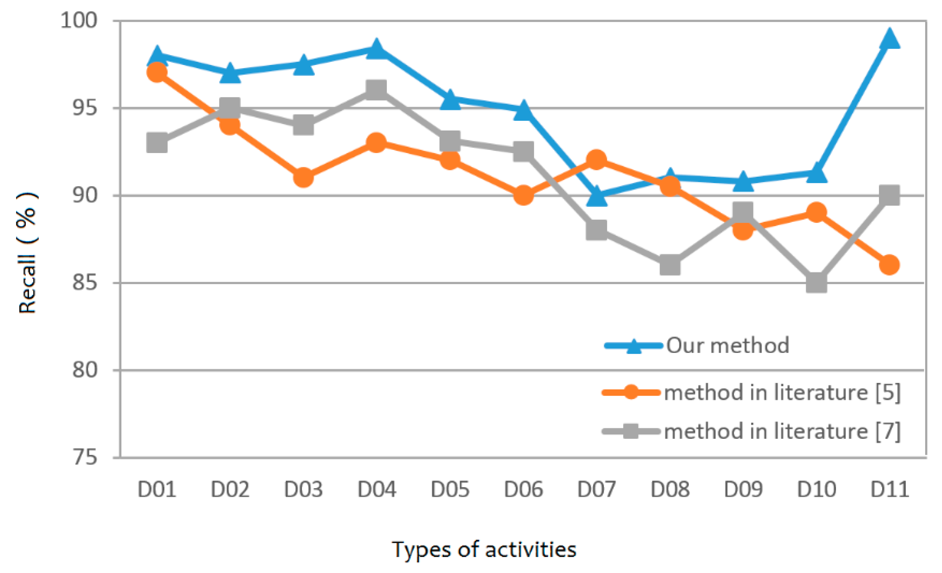
Based on the previously extracted Sacc, SD, DAPT and IoP, and the deep neural network classifier method proposed in literature [33], we classified D01–D11. As shown in Figure 15, we compare our method with literature [5,7]. These three methods are run on SisFall. It can be seen that the method of [5] is slightly better than our method in the identification of D07. However, the recognition effects of our method are better than the other two methods in most cases.

4. Conclusions

Wearable device is a promising method for collecting acceleration data of human body, that can be used for behavior recognition. This paper focused on investigating the feature extraction method based on wearable devices with single acceleration sensor. We associate Kalman filter algorithm with genetic algorithm for data pre-processing, which greatly reduces the amount of calculation. Then, we propose SD, IoP and DAPT as acceleration feature values that can be extracted from processed data sets. The experiments indicate that the source data filtered by KGA algorithm is more compact and the acceleration values in the three directions are more distinct. SD, DAPT and IoP are very obvious for the discrimination of seven different movements.

References

- Hussain, S.; Kang, B.H.; Lee, S. A Wearable Device-Based Personalized Big Data Analysis Model. In Ubiquitous Computing and Ambient Intelligence. Personalisation and User Adapted Services; Springer: Berlin/Heidelberg, Germany, 2014; pp. 236–242. [Google Scholar]
- Hsu, Y.L.; Yang, S.C.; Chang, H.C.; Lai, H.-C. Human Daily and Sport Activity Recognition Using a Wearable Inertial Sensor Network. IEEE Access 2018, 6, 1–14. [Google Scholar] [CrossRef]
- Wilson, C.; Hargreaves, T.; Hauxwell-Baldwin, R. Smart homes and their users: A systematic analysis and key challenges. Pers. Ubiquitous Comput. 2015, 19, 463–476. [Google Scholar] [CrossRef] [Green Version]
- Song, F.; Zhou, Y.; Wang, Y.; Zhao, T.; You, I.; Zhang, H. Smart Collaborative Distribution for Privacy Enhancement in Moving Target Defense. Inf. Sci. 2019, 479, 593–606. [Google Scholar] [CrossRef]
- Chen, Y.; Shen, C. Performance Analysis of Smartphone-Sensor Behavior for Human Activity Recognition. IEEE Access 2017, 5, 3095–3110. [Google Scholar] [CrossRef]
- Song, F.; Zhu, M.; Zhou, Y.; You, I.; Zhang, H. Smart Collaborative Tracking for Ubiquitous Power IoT in Edge-Cloud Interplay Domain. IEEE Internet Things J. 2020, 7, 6046–6055. [Google Scholar] [CrossRef]
- Janidarmian, M.; Fekr, A.R.; Radecka, K.; Zilic, Z. A Comprehensive Analysis on Wearable Acceleration Sensors in Human Activity Recognition. Sensors 2017, 17, 529. [Google Scholar] [CrossRef]
- Song, F.; Zhou, Y.; Chang, L.; Zhang, H. Modeling Space-Terrestrial Integrated Networks with Smart Collaborative Theory. IEEE Netw. 2019, 33, 51–57. [Google Scholar] [CrossRef]
- Wang, A.; Chen, G.; Yang, J.; Chang, C.-Y.; Zhao, S. A Comparative Study on Human Activity Recognition Using Inertial Sensors in a Smartphone. IEEE Sens. J. 2016, 16, 4566–4578. [Google Scholar] [CrossRef]
- Lara, O.D.; Labrador, M.A. A Survey on Human Activity Recognition using Wearable Sensors. IEEE Commun. Surv. Tutor. 2013, 15, 1192–1209. [Google Scholar] [CrossRef]
- Su, X.; Caceres, H.; Tong, H.; He, Q. Online Travel Mode Identification Using Smartphones with Battery Saving Considerations. IEEE Trans. Intell. Transp. Syst. 2016, 17, 2921–2934. [Google Scholar] [CrossRef]
- Ling, B.; Intille, S.S. Activity Recognition from User-Annotated Acceleration. Data Proc. Pervasive 2004, 3001, 1–17. [Google Scholar]
- Priyanka, K.; Tripathi, N.K.; Peerapong, K. A Real-Time Health Monitoring System for Remote Cardiac Patients Using Smartphone and Wearable Sensors. Int. J. Telemed. Appl. 2015, 2015, 1–11. [Google Scholar]
- Chao, C.; Shen, H. A feature evaluation method for template matching in daily activity recognition. In Proceedings of the 2013 IEEE International Conference on Signal Processing, Communication and Computing (ICSPCC 2013), KunMing, China, 5–8 August 2013; pp. 1–4. [Google Scholar]
- Maekawa, T.; Kishino, Y.; Yasushi, S. Activity recognition with hand-worn magnetic sensors. Pers. Ubiquitous Comput. 2013, 17, 1085–1094. [Google Scholar] [CrossRef]
- Cheng, J.; Amft, O.; Bahle, G.; Lukowicz, P. Designing Sensitive Wearable Capacitive Sensors for Activity Recognition. IEEE Sens. J. 2013, 13, 3935–3947. [Google Scholar] [CrossRef]
- Barshan, B.; Yüksek, M.C. Recognizing Daily and Sports Activities in Two Open Source Machine Learning Environments Using Body-Worn Sensor Units. Comput. J. 2013, 57, 1649–1667. [Google Scholar] [CrossRef]
- Zhang, M.; Sawchuk, A.A. A feature selection-based framework for human activity recognition using wearable multimodal sensors. In Proceedings of the 13th International Conference on Ubiquitous Computing (UbiComp 2011), Beijing, China, 17–21 September 2011; pp. 92–98. [Google Scholar]
- Dinov, I.D. Decision Tree Divide and Conquer Classification. In Data Science and Predictive Analytics; Springer: Berlin/Heidelberg, Germany, 2018; pp. 307–343. [Google Scholar]
- Aziz, O.; Russell, C.M.; Park, E.J.; Robinovitch, S.N. The effect of window size and lead time on pre-impact falls detection accuracy using support vector machine analysis of waist mounted inertial sensor data. In Proceedings of the 2014 36th Annual International Conference of the IEEE Engineering in Medicine and Biology Society, Chicago, IL, USA, 26–30 August 2014; pp. 30–33. [Google Scholar]
- Diep, N.N.; Pham, C.; Phuong, T.M. A classifier based approach to real-time falls detection using low-cost wearable sensors. In Proceedings of the 2013 International Conference on Soft Computing and Pattern Recognition (SoCPaR), Hanoi, Vietnam, 15–18 December 2015; pp. 14–20. [Google Scholar]
- Jian, H.; Chen, H. A portable falls detection and alerting system based on k-NN algorithm and remote medicine. China Commun. 2015, 12, 23–31. [Google Scholar] [CrossRef]
- Song, F.; Ai, Z.; Zhou, Y.; You, I.; Choo, R.; Zhang, H. Smart Collaborative Automation for Receive Buffer Control in Multipath Industrial Networks. IEEE Trans. Ind. Inform. 2020, 16, 1385–1394. [Google Scholar] [CrossRef]
- Foody, G.M. RVM-based multi-class classification of remotely sensed data. Int. J. Remote Sens. 2008, 29, 1817–1823. [Google Scholar] [CrossRef]
- Anguita, D.; Ghio, A.; Oneto, L.; Parra, X.; Reyes-Ortiz, J.L. Human Activity Recognition on Smartphones Using a Multiclass Hardware-Friendly Support Vector Machine Ambient Assisted Living and Home Care. In Ambient Assisted Living and Home Care; Springer: Berlin/Heidelberg, Germany, 2012; pp. 216–223. [Google Scholar]
- Martín, H.; Bernardos, A.M.; Iglesias, J.; Casar, J.R. Activity logging using lightweight classification techniques in mobile devices. Pers. Ubiquitous Comput. 2013, 17, 675–695. [Google Scholar] [CrossRef]
- Song, F.; Ai, Z.; Zhang, H.; You, I.; Li, S. Smart Collaborative Balancing for Dependable Network Components in Cyber-Physical Systems. IEEE Trans. Ind. Inform. 2020. [Google Scholar] [CrossRef]
- Nukala, B.T.; Shibuya, N.; Rodriguez, A.I.; Nguyen, T.Q.; Tsay, J.; Zupancic, S.; Lie, D.Y.C. A real-time robust falls detection system using a wireless gait analysis sensor and an Artificial Neural Network. In Proceedings of the 2014 IEEE Healthcare Innovation Conference (HIC), Seattle, WA, USA, 8–10 October 2014; pp. 219–222. [Google Scholar]
- Angela, S.; López, J.; Vargas-Bonilla, J. SisFall: A Fall and Movement Dataset. Sensors 2017, 17, 198. [Google Scholar]
- Digital Signal Processing Formula Variable Program (four)-Butterworth Filter (On). Available online: https://blog.csdn.net/shengzhadon/article/details/46784509 (accessed on 7 July 2015).
- Kalman, R.E. A New Approach to Linear Filtering and Prediction Problems. J. Fluids Eng. 1960, 82, 35–45. [Google Scholar] [CrossRef] [Green Version]
- Xianglin, W.; Jianwei, L.; Yangang, W.; Chaogang, T.; Yongyang, H. Wireless edge caching based on content similarity in dynamic environments. J. Syst. Archit. 2021, 102000. [Google Scholar] [CrossRef]
- Bingqian, H.; Wei, W.; Bin, Z.; Lianxin, G.; Yanbei, S. Improved deep convolutional neural network for human action recognition. Appl. Res. Comput. 2019, 36, 3111–3607. [Google Scholar]
Figure 1.
Wearing of accelerometer and directions of coordinate axes.
Figure 2.
Diagram of the algorithm.
Figure 3.
Acceleration data of D01: (a) x axis acceleration; (b) y axis acceleration; (c) z axis acceleration; (d) Sacc superposition acceleration.
Figure 4.
Diagram of source data.
Figure 5.
Diagram of low-pass filter.
Figure 6.
Diagram of Kalman filter.
Figure 7.
Diagram of KGA.
Figure 8.
Diagram of features in D03: (a) Sacc over time; (b) SD over time; (c) DAPT over time; (d) IoP over time.
Figure 9.
Diagram of features in D04: (a) Sacc over time; (b) SD over time; (c) DAPT over time; (d) IoP over time.
Figure 10.
Diagram of features in D05: (a) Sacc over time; (b) SD over time; (c) DAPT over time; (d) IoP over time.
Figure 11.
Diagram of features in D06: (a) Sacc over time; (b) SD over time; (c) DAPT over time; (d) IoP over time.
Figure 12.
Diagram of features in D07: (a) Sacc over time; (b) SD over time; (c) DAPT over time; (d) IoP over time.
Figure 13.
Diagram of features in D08: (a) Sacc over time; (b) SD over time; (c) DAPT over time; (d) IoP over time.
Figure 14.
Diagram of features in D11: (a) Sacc over time; (b) SD over time; (c) DAPT over time; (d) IoP over time.