
Wind Put Barrier Options Pricing Based on the Nordix Index


1
Departamento de Estudios Contable y Financiero, Escuela de Economía y Finanzas, Universidad Icesi, 760008 Cali, Colombia
2
E.T.S. de Ingeniería Industrial, University of Castilla—La Mancha, 13071 Ciudad Real, Spain
*
Author to whom correspondence should be addressed.
Energies 2021, 14(4), 1177; https://doi.org/10.3390/en14041177
Submission received: 31 December 2020
/
Revised: 30 January 2021
/
Accepted: 7 February 2021
/
Published: 23 February 2021
(This article belongs to the Special Issue Mathematical and Statistical Models for Energy with Applications)
Abstract
:Wind power generators face risks derived from fluctuations in market prices and variability in power production, generated by their high dependence on wind speed. These risks could be hedged using weather financial instruments. In this research, we design and price an up-and-in European wind put barrier option using Monte Carlo simulation. Under the existence of a structured weather market, wind producers may purchase an up-and-in European wind barrier put option to hedge wind fluctuations, allowing them to recover their investments and maximise their profits. We use a wind speed index as the underlying index of the barrier option, which captures risk from wind power generation and the Autoregressive Fractionally Integrated Moving Average (ARFIMA) to model the wind speed. This methodology is applied in the Colombian context, an electricity market affected by the El Niño phenomenon. We find that when the El Niño phenomenon occurs, there are incentives for wind generators to sell their energy to the system because their costs, including the put option price, are lower than the power prices. This research aims at encouraging policymakers and governments to promote renewable energy sources and a financial market to trade options to reduce uncertainty in the electrical system due to climate phenomena.
1. Introduction
Weather derivatives are used to manage the economic consequence of non-catastrophic weather events on companies’ performance [1,2,3,4,5,6,7,8,9,10,11,12,13]. Given there is no standardised pricing model for weather derivatives, recent studies have developed different pricing models using underlying indices derived from climatic variables like temperature [2,4,5,8,10,11,12,14,15,16], irradiance [17], rainfall [3,6] and wind [18,19,20,21]. The derivatives most used are options [3,4,5,6,7,8,11,15,16,22,23], futures [2,10,12] and swaps [15,24].
Simultaneously, many countries started a deregulation process of their electrical systems, which has been accompanied by a rapidly growing presence of small generators whose technologies are based on renewable energy sources [25]. The increase in the share of these sources in the generation portfolio is essential to reduce risk related to unexpected weather conditions, which are propitiated by climate phenomena such as El Niño/La Niña. In South American countries such as Colombia, the main effects of El Niño are low precipitation rates and constant high temperatures, which have had significant repercussions since the power generation park is mostly hydraulic [26]. In this context, it is relevant for the stability of the power system that the government incentivises the use of renewable resources, such as wind generation [20], taking into account that it exhibits the fastest growth worldwide [27].
Nevertheless, wind power generators face risks derived from both fluctuations in market prices, as any other power generator, and variability in power production, which is explained due to their high dependence on wind speed. To mitigate these risks, wind generators could use wind derivatives [18,19,20,21]. Yamada [19] proposes a wind derivative that predicts the errors for wind speed based on a nonparametric regression in the Japanese context. Contreras and Rodríguez [20] recommend a methodology for pricing European wind put options, considering price volatility and its behaviour as a martingale, and they have applied their methodology to the Colombian context. Benth et al. [21] model the electricity prices using a normal inverse Gaussian process and the wind speed power and production through two Ornstein–Uhlenbeck processes. They propose Quanto options because these allow considering volatility that comes from more than one factor. Similarly, Hess [28] prices a wind power future based on a wind power production index using an Ornstein-Uhlenbeck model to capture the stochastic process in wind power production.
Wind power futures can hedge risk related to the wind generation resulting from stochastic wind speed, and producers are willing to pay a premium to transfer this risk, as Gersema and Wozabal [29] show in their equilibrium model for the European context. Additionally, Zhang, Wang and Wang [30] and Xiao, Wang, Wang and Wu [31] use barrier options in electricity markets to face risk on the demand and supply sides, respectively, using the price of electricity as an underlying asset.
In this sense, we use a wind speed index as the underlying index of the barrier option, which captures this risk from wind power generation, which is a novelty approach that does not consider the traditional Black–Scholes valuation methodology. Therefore, the goal of this paper is to design and price an up-and-in European wind barrier put option based on the Nordix index, using ARFIMA to model the wind speed. The purpose of the barrier put option is that the producers of wind energy cover their costs, selling the energy at the strike price when energy prices are low. The contribution to the literature is focused on proposing a new methodological development for barrier put option pricing based on a weather index considering both stochastic wind speed risks and volatility power energy prices with an application in the Colombian context, which is affected by El Niño/La Niña phenomena that impact wind speed and power prices.
This work can complement previous proposals to enhance the viability and profitability of wind power generators by providing them alternatives to cover both stochastic wind speed risks and volatility power energy prices in sum with operational optimisation strategies [32,33,34]. For instance, Bui et al. [33] propose to evaluate the appropriate location of wind farm systems based on stochastic optimisation, considering a large number of scenarios through an algorithmic methodology to optimise the set-points and to reduce the uncertainly in the outcome power.
In this line, Cobos et al. [34] suggest a scheduling methodology to cope with uncertainty related to intermittency and volatility in wind power generation using conventional fast-acting generating units like gas turbines and combined-cycle units, characterised by their high cost, to optimise the operation of the system based on a two-stage optimisation strategy that considers the market reserve. Similarly, Bludszuweit and Domínguez-Navarro [32] design and recommend an energy-storage-sizing system to reduce uncertainty based on the risk in wind power generation because of their stochastic behaviour. Combining these strategies with an up-and-in European wind barrier put option based on the Nordix index wind power, producers can optimise their decision-making process and facilitate the transition to renewable energies by improving their certainty profitability.
The paper is organised as follows. Section 2 includes a description about barrier options, their use in the electricity markets, barrier options based on weather indexes and their pricing. In Section 3, the methodology used to calculate the price of the wind barrier put option is described. Section 4 presents a real case study from the Colombian market, and finally, Section 5 discusses the results.
2. Barrier Options
A European option gives the holder the right, but not the obligation, to buy (call) or sell (put) an underlying asset at a fixed price at the moment of maturity of the contract option. In particular, a barrier option is a special type of financial derivative with a defined limit, which is named barrier. This barrier is used in order to determine the value of the option. In general, barrier options are cheaper than traditional ones [35]. The payoff of the barrier option depends on whether the underlying asset’s price reaches a definite level, denominated a barrier , during the option’s life [36]. This kind of options can be classified as knock-in options or knock-out options [36].
The in options become active when the underlying asset’s price reaches the barrier. In the case that the option is priced below the barrier, the barrier option is named up and in option, and if the option is priced above the barrier, the barrier option is known as down and in option [36]. If the underlying’s asset price does not reach the barrier, the option will expire without value [36].
Similarly, the out options are active from the beginning but become inactive when the underlying’s price reaches the barrier. These options also can be up or down. An up and out option ceases to exist if the barrier level is higher than the underlying’s asset price, while a down and out option ceases to exist if the barrier is lower than the underlying’s asset price [36]. Hull [36] derived a formula similar to Black–Scholes’s in order to price put and call barrier options.
2.1. Barrier Options in Electricity Markets
In an electricity market context, barrier options have been used to manage the risk related to power market demand and supply [30,31], from the consumers’ demand side, through the incorporation of interruptible electricity contracts with utilities [30] and, from the supply side, through hedging the risks of both power generation and market prices faced by wind power producers [31].
Zhang et al. [30] proposed the use of an interruptible electricity contract (IEC), which is a power contract with the characteristics of a barrier option that allows improving risk management in the electric power markets, which are characterised by its low demand elasticity. They suggested that interruptible electricity contracts can reduce the load when the electricity price reaches a certain barrier price agreed in the contract, increasing the demand elasticity. The mechanism used implies that costumers and utility can cover their positions using forwards and call options. Customers buy electricity futures but simultaneously cover themselves through the sale of a call option, which can be exercised if the price of power reaches a certain barrier defined in the contract. On the other hand, utilities play an inverse strategy, selling electricity futures and buying call options [30].
This hedging strategy provides utility and costumers the right to reduce the supply if the electricity prices reach the barrier price. To model electricity prices, Zhang et al. [30] used a hybrid model based on the mean regression model and a jump model. Additionally, to prove the effectiveness of the interruptible electricity contracts, they priced the option using the Monte Carlo valuation method, considering that the underlying asset is the electricity price, which does not follow a Brownian motion model, a fundamental assumption of the traditional pricing Black-Scholes model. They used and modelled historical data of the New England power market from 2000 to 2001, including market clearing prices and system load rates to check the validity of the proposed method. They found a relative error between the actual option value and the option value calculated by the proposed method to be less than 5%, proving the effectiveness of the proposed methodology.
Now, in a supply context, Xiao et al. [31] proposed the use of a knock-in put barrier option for wind power in order to hedge and manage risk from both power generation associated with wind speed and market price volatility due to power’s fluctuation and randomness faced by wind power producers. They used wind power traded price and equivalent traded quantity as the underlying assets, which captures risks from market price and power generation, to provide an optimal purchasing framework strategy to hedge power at prices no less than a fixed strike price during the option life; these strategies were analysed in bilateral contract and pool marker scenarios. In this case, the barrier option gives the right to the wind power producers to sell power at prices no lower than the strike price when the price falls below the barrier price level. These authors proved the applicability of the proposed barrier option in the Iberian market and showed that barrier option and bilateral contract are optimal, since their simultaneous use allows for flexibility in the use of the contracts and lowers prices [31].
2.2. Barrier Options Based on Weather Indexes
Previous works used the price of electricity as the underlying asset [30,31]. Nevertheless, wind power generators are interested in long-term forecasts of wind speed that lead to managing the risk associated with this variable. Based on that assumption, we propose as a mechanism of risk management for wind producers barrier option pricing based on the Nordix index. In this case, the underlying index is this wind index.
It is important to note that weather derivative pricing does not use the Black–Scholes model [37,38,39]. According to Botoş and Ciumaş [39], some of the reasons why the Black–Scholes model is not suitable for the valuation of weather derivatives are (1) the underlying asset (rain, precipitation, wind speed) has no direct value to the price of derivative, and it is not standard tradable, so its price cannot be free of financial risks; (2) the evolution of the weather is determined by meteorological and geological factors, which makes the variable take certain values inside narrow intervals; and (3) weather does not exhibit the random nature of financial assets, and its inherent nature makes it predictable in the short term and makes it random around historical averages in the long term.
For our pricing proposal, the following items are described below: wind speed modelling methods, Nordix index, structuring of the chosen barrier option and its operation.
2.2.1. Wind Speed Modelling
Some statistical approaches are viable in order to model meteorological variables [40]. For example, time series have been widely used to forecast wind speeds by fitting a Gamma Auto-regressive (GAR) model [41], an auto-regressive gamma model [42], Auto-regressive Moving Average (ARMA) and Autoregressive Moving Average-generalized Autoregressive Conditional Heteroskedasticity (ARMA-GARCH) models [43] and an Autoregressive Fractionally Integrated Moving Average-fractionally Integrated Generalized Autoregressive Conditional Heteroskedasticity (ARFIMA-FIGARCH) model [40]. Among these models, ARFIMA models have been widely used in hydrology; in particular, Hurst [44] was the first to introduce a long-memory process where the studies of Hosking [45], Beran [46], Bailie [47] and Palma [48] can be highlighted.
ARFIMA models are long-memory processes that exhibit a stationary behaviour and their autocorrelation functions decay more slowly compared to a short-memory process, which means that this kind of process presents a type of long-running dependence. Therefore, the parameterisation of ARFIMA models is connected to ARMA models [40], which are widely used for short-memory processes.
2.2.2. Nordix Index
Index modelling is one of the most common valuation methods of weather derivatives. In the case of wind, the most commonly referenced index on which wind derivatives are written is the Nordix wind speed index. The US Futures Exchange uses the Nordix index, and it is calculated on the deviations of the daily wind speed from a 20-year mean value [49]. These deviations are aggregated over a measurement period. Additionally, a value of 100 is added to the sum of the deviations [50].
The mathematical formulation of the Nordix index is that if we let W(t) be the average daily wind speed measured on day t and the mean of the last 20 years’ wind speeds for day t, the Nordix index, , over the period is defined as:
2.2.3. Put Barrier Option Pricing Structuring
We propose the pricing of an up and in put barrier option. According to Cao and Wei [51], the payoff of a traditional European wind put option written on the Nordix index can be defined as:
where , based on the definition of the barrier option with duration , is expressed as:
where is the Nordix index’s barrier and K refers to the strike index, defined as a particular value of the Nordix index. For example, it can be estimated with historical information about the Nordix index, as shown in [40].
refers to the monetary value of one point of the Nordix index, and it is expressed in $/kWh per Nordix index. The tick size can be defined in the over-the-counter (OTC) market using different criteria.
Based on the description above, to price wind derivatives, we design and price an up-and-in European wind put barrier option based on the Nordix index. The novelty is related to the use of wind barrier options based on weather indexes in the electricity market, where those indexes cannot be priced through the traditional methodology proposed by Black and Scholes. In this way, we propose a theoretical development to price this type of option, whose underlying asset is the Nordix wind index, associated with wind speed deviations.
We suggest the use of the time series ARFIMA to model and characterise the wind speed, and price the option through simulations of many possible scenarios of average daily wind speeds coming from the parameter estimates of the ARFIMA model. This financial instrument can help wind power generators in such a way that they may purchase an up-and-in European wind put barrier option to hedge against fluctuations in wind production to recover their investments more quickly and maximise their profits. It also can promote the development of wind power projects to guarantee constant cash flows that hedge against the risks associated with the variability of wind speed.
3. Methodology
We set an up-and-in European wind put barrier option based on the modelling of the wind speed through the Nordix index, an index that allows us to include the risks associated with wind power generation, taking into account that the generators require speed ranges of wind to make generation viable. In this sense, we proposed to model the daily wind speed from an ARFIMA model in order to simulate 10,000 repetitions of wind speed. With these simulations, we built the underlying Nordix index to structure the option based on the wind speed requirements of the turbine, and finally, we monetarily valued the option from the calculation of a tick value.
The up-and-in European wind put barrier option is for one location in Colombia, during the summer season. It is set for the meteorological station with the highest wind speed in Colombia, Almirante Padilla, located in the Department of Guajira. In general, wind derivatives are useful for power generators who are interested in developing wind projects to guarantee constant cash flows that hedge against the risks associated with the variability of wind speed.
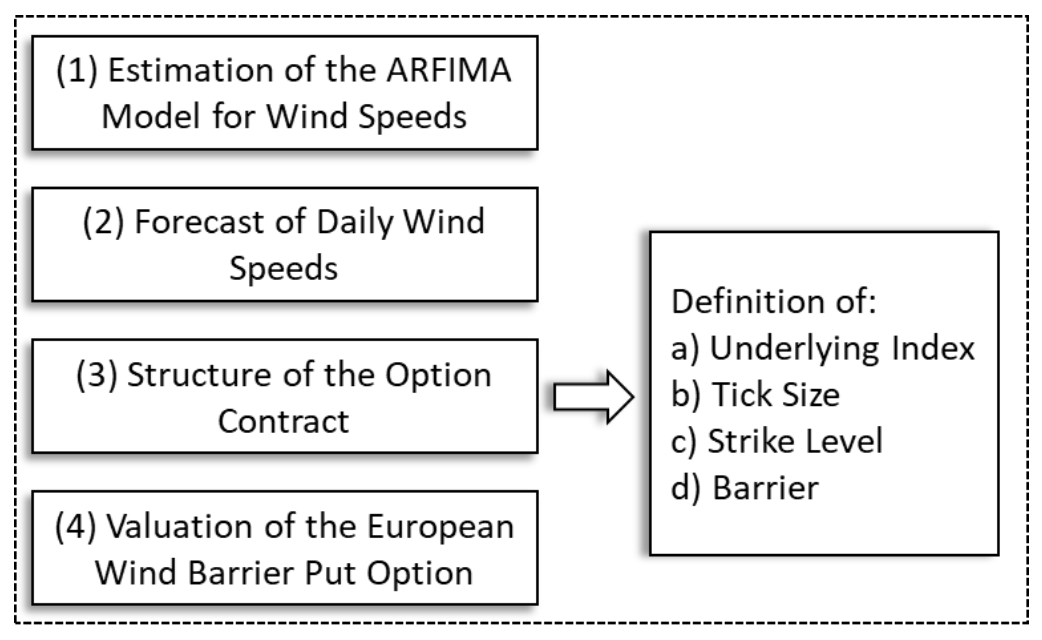
Figure 1 presents the steps of the methodology used in the calculation of the value of European put options.
The four steps for pricing a European wind put barrier option are detailed in the following sections.
3.1. Estimation of the ARFIMA Model for Wind Speeds
ARFIMA models are long-memory processes that exhibit a stationary behaviour, and their autocorrelation functions decay more slowly compared to a short-memory process, which means that this kind of process presents a type of long-running dependence.
The ARFIMA model can be specified as:
where .
The short-term ARMA process captures the short-term effects. Likewise, the long-term effects are captured by integrating the short-term ARMA process fractionally.
The estimation method of an ARFIMA model is the maximum likelihood [52]. An ARFIMA model has the d parameter to establish the long-run dependence and the ARMA parameters, p and q, to show short-run dependence. It must be verified that the confidence interval for the fractional-difference parameter d includes numbers that are smaller than 0.5 in order to prove that the series is stationary and that the parameters are significant at a 5% significance level. Finally, spectral densities are analysed in order to test the model’s ability.
Wind speed time series present seasonal effects; therefore, they require to be transformed and differentiated. In addition, given that the autocorrelation function decays slowly, an ARFIMA model is chosen to fit the data.
3.2. Forecast of Daily Wind Speeds
The ability of the ARFIMA model to forecast can be evaluated calculating the forecasting error [53]. The daily forecast error is given by:
where and . refer to the actual and forecasted daily wind speeds, respectively. Monthly forecast errors are calculated as averages of the daily forecast errors.
3.3. Structure of the Option Contract
The wind put barrier option specifies the underlying index (Nordix), the strike index (K), the tick size (t) and the tick value for each meteorological station
The Nordix index is calculated based on simulations of realisations of average daily wind speeds coming from the parameter estimates of the ARFIMA model of daily wind speeds.
The strike index (K) is estimated for the yearly average Nordix index for the estimation period [40].
In the case of the tick size, we propose that it must be estimated as the quotient of the annual payment availability of a wind generator who presents the corresponding capacity and the annual estimated energy produced by a turbine with the corresponding capacity. The payment availability is chosen from a quantity set that varies from $100 USD to $1750 USD. In addition, the annual estimated energy is calculated for each size of turbine, as a function of three variables: (i) the air density expressed in kg/m3, (ii) the area covered by the blades of the generator expressed in m2 and (iii) the average of the cube of the wind speed. The area covered by the blades depends on the characteristics of the wind unit such as capacity, height of the tower, diameter, etc.
Finally, the calculation of the tick value is done using the mathematical expression defined in Equation (3). In this work, a descriptive analysis of the Nordix index has been done in order to define the barrier of this index , and the 50th percentile of the Nordix index is proposed to be taken as the barrier.
3.4. Valuation of the European Wind Put Barrier Option
For each simulation of wind speed using the ARFIMA model, the monetary payoff from the contract is the product of the tick value and the corresponding tick size. The value of the wind put barrier option is calculated as the average value of the simulations.
4. Case Study
The case study focuses on a specific location in the Colombian Department of La Guajira, which is located in the extreme north of Colombia, and the Caribbean plain, in the northernmost part of South America. The territory corresponding to the peninsula of Guajira is semi-desertic, with sparse vegetation and some mountainous areas that do not exceed 50 m above sea level [54].
La Guajira is one of the territories in South America with the highest wind energy potential and with an installable capacity of around 18 GW. In this department, the highest wind regimes that Colombia receives during the whole year are concentrated, with average speeds close to 9 m/s (at 80 m of height) and prevailing east-west direction [55].
The wind speeds used in this study are collected from the Instituto de Hidrología, Meteorología y Estudios Ambientales (IDEAM), the entity in charge of managing meteorological information in order to give technical support on the sustainable use of natural resources in Colombia.
The meteorological station in La Guajira in named Almirante Padilla. For this station, daily wind speed information is available for the period 2000–2010. However, the estimation year is 2009 and is used to estimate the ARFIMA model, while the information corresponding to 2010 is used for forecasting. The main statistical values of the daily average wind speeds for the Almirante Padilla station are presented in Table 1.
The Almirante Padilla station presents the maximum level of wind speed at 8.3 m/s, and its daily average is 3.72 m/s. On average, the station meets the minimum wind speed required for plant operation, which is 3 m/s.
4.1. Estimation of the ARFIMA Model for Wind Speeds
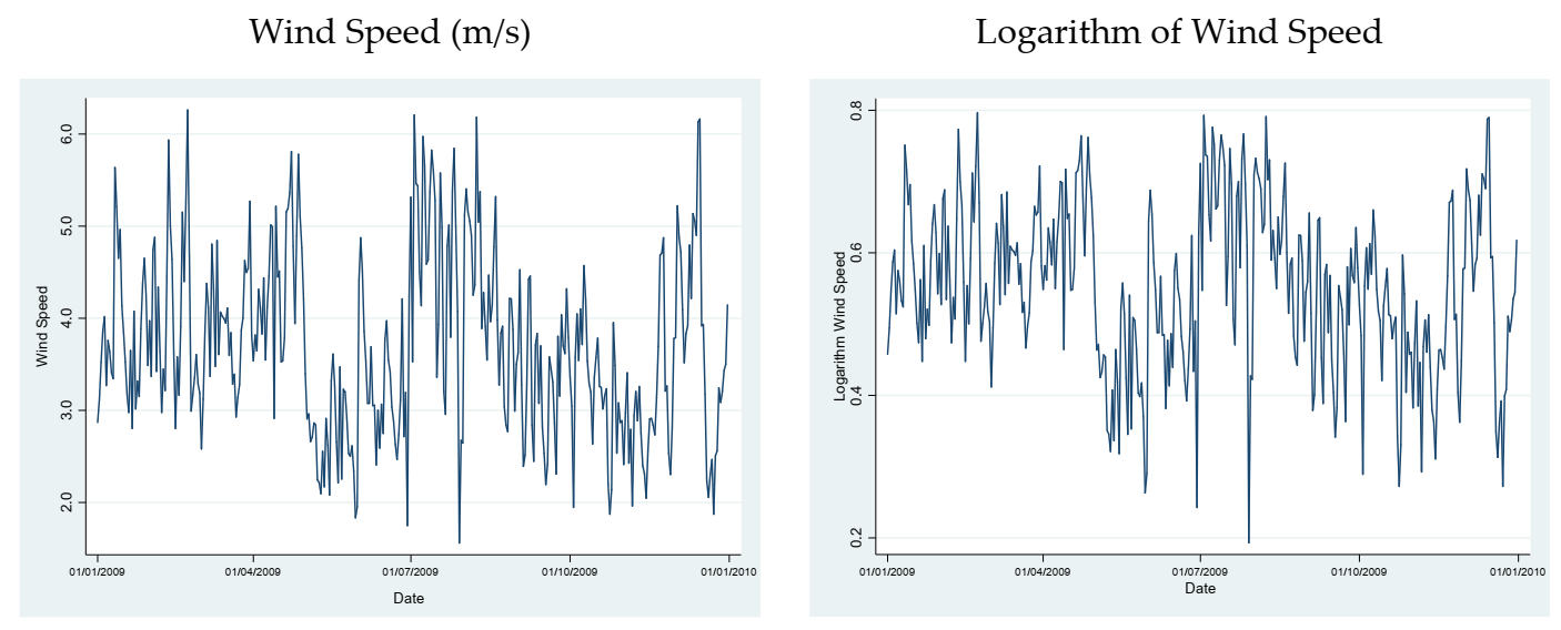
Figure 2 presents the time series of wind speeds and its logarithm for the Almirante Padilla station in the year 2009.
Wind speed time series data are transformed with the logarithmic function to achieve stationarity. A seasonal effect is observed approximately each quarter, which is explained by the number of days of the winter and summer seasons. Therefore, the logarithm of the wind speed is differentiated using the ninetieth seasonal difference in order to remove this seasonal effect.
We consider an AR(1) model for this series, based on the behaviour of simple and partial autocorrelation functions. The autocorrelation function does not show a behaviour that allows us to estimate moving average terms in the model. The AR(1) model is nested in the ARFIMA model, which is presented in Table 2.
All parameters are significant at the 5% significance level. The estimated value for d is greater than zero, evidencing long-term dependence.
Figure 3 presents the spectral densities computed for the ARMA and ARFIMA models for both short and long terms.
It is observed that in the case of the ARMA model, the short- and long-memory spectral densities are almost the same, indicating that the ARMA model mixes up the long-run and short-run effects.
In contrast, the short- and long-term spectral densities of the ARFIMA model are different for frequencies close to zero. In addition, unlike the long-memory ARFIMA, the short-memory ARFIMA can capture both low- and high-frequency components in its spectral density. With these estimates, we can test the flexibility of the ARFIMA model to capture the long-run dependence.
4.2. Forecast of Daily Wind Speeds
Daily wind speeds up to one year ahead are forecasted with the ARFIMA model. Table 3 shows the monthly average errors of the ARFIMA model estimated for the three months that correspond to the summer season.
The average monthly error in summer is 7.027%, where the minimum weekly error is 4.672% for the third month of the year, and the maximum is 9.37% for the second month of the year.
4.3. Structure of the Option Contract
The features of the up-and-in European wind put barrier option for the Almirante Padilla station are tick size (depending of the capacity of the farm), strike index and tick value.
The summer season has been chosen because during this time of the year, wind speeds are higher compared to the ones in winter, producing higher Nordix indices. This data behaviour produces a higher pricing of the put options during summer. Note that in Colombia the summer period is associated with the months of the first quarter of the year.
Table 4 presents the technical characteristics of the wind turbine with a capacity of 1300 kW.
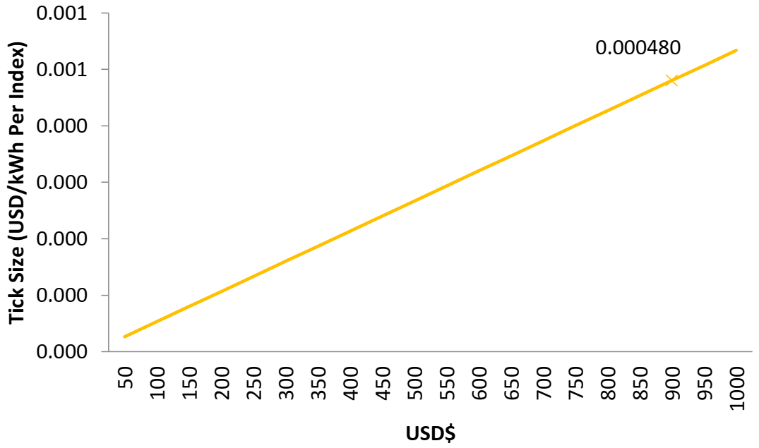
The tick size is defined for the size of wind turbine. Figure 4 presents the behaviour of the tick size, depending on the availability of payment (in USD).
It is observed that the tick size increases with the payment availability. The payment availability defined for the defined size of wind turbine is $850 USD.
This choice seeks to incentivise generators to buy these kinds of instruments, where the price of the option is greater depending not only on the size of the wind turbine but also on the daily wind speed for the location where the wind turbine is placed. Those power generators who have wind turbines located in places that present more dispersed daily wind speeds with respect to the average daily wind over the past 10 years end up having to pay more for the put option.
The strike index is calculated as the historical yearly average Nordix index for the summer season and has a value of 215.8. The tick value is calculated following Equation (3), taking a value of 125.4 as the Nordix barrier.
In summary, the structure of the up-and-in European wind put barrier option is presented in Table 5.
4.4. Valuation of the European Wind Put Barrier Option
The price of the wind put barrier option calculated for Almirante Padilla station for the selected wind turbine is $0.033144 USD/kWh.
Clearly, the annual income of a wind producer depends on the annual electricity production, which is determined by the wind speed at the location. Therefore, this means that weather variability leads to volume risk. Consequently, investing in an up-and-in European wind put barrier option would be of interest for a wind producer who wants to hedge the risk of low production over a given period, in this case during the summer of 2010.
Although the calculations of the traditional option are not presented, in this study, we compared the value of the barrier option for the tick size and we obtained, in all cases, an outcome that evidences that the up-and-in European wind put barrier options are 17% cheaper than the traditional put options. In this way, the payments of the barrier options obtained represent a significant cost reduction for the generators, independent of their size.
5. Results and Discussion
Weather derivatives are used to manage the impact of weather risk events with a high probability of occurrence. In this work, an ARFIMA model of wind speed was estimated and used to forecast and simulate daily wind speeds in order to estimate the Nordix index for the summer season. This index was used as underlying index of an up-and-in European wind put barrier option that was structured and priced using a Monte Carlo simulation in the spirit of Campbell and Diebold [56]. This simulation was done for the meteorological station with the highest wind speed in Colombia.
Wind producers may purchase an up-and-in European wind put barrier option to hedge against fluctuations in wind production to recover their investments more quickly and maximise their profits, but it all depends on whether the climate is being affected by El-Niño-related phenomenon.
Figure 5 and Figure 6 present a comparison between electricity prices, wind generation cost and prices of wind put barrier options, with and without the El Niño phenomenon, respectively. In particular, Figure 5 shows the energy prices between 1 January and 31 March 2016, where this quarter was marked by the El Niño phenomenon. Figure 6 shows the energy prices between 1 April and 30 June 2016, where this quarter was a typical period without such phenomenon. In addition, the wind put barrier option used is the one corresponding to the biggest capacity station, because we consider that this wind generator could be the interested in selling their energy to the system.
It is observed that the prices increase significantly in Colombia in the periods with the El Niño phenomenon, which can be explained due to the high temperatures and low precipitations that affect hydroelectric plants.
When the El Niño phenomenon occurs, there is an incentive for wind generators to sell their energy to the system, because the sum of the generation costs and the put option price is lower than the power price. In this way, when the producer hedges using an up-and-in European wind put barrier option, they recover their investment and costs, hedging the risk of low wind speed levels. However, in periods without the El Niño phenomenon, these wind generators do not have much incentive to exercise the put option, because the power prices are lower than their costs on most days.
Although the use of weather derivatives presents great advantages, it is important to note that it is expected that this market will be illiquid because of the location-specific features and the limited number of agents interested in trading.
The structuring of a weather derivatives market requires governments to encourage the use of renewable sources in a complementary way to traditional generation and to promote the use of financial instruments based on weather, such as weather options, in order to reduce the uncertainty of the electrical system caused by climate phenomena such as El Niño/La Niña. In particular, wind power generators, whose profits and revenues could be affected by weather risks, can invest in the weather derivatives market and have the right to sell their energy, making the recovery of their investments possible, and hedging their cash flows against the risks associated with the variability of wind speed. This proposal can complement operational optimisation strategies to reduce uncertainty and facilitate the producers’ decision-making processes by improving their profitability estimation, helping in the transition to renewable energy sources.
Finally, for any context, the future of weather derivatives is uncertain, mainly due to three aspects. First, the availability of reliable data on wind speeds is limited. Second is the uncertainty associated with the operative process. Third, the recognition of the importance of weather derivatives to provide new opportunities in dealing with the weather for industries directly or indirectly affected by weather risks has yet to be fully developed. Additionally, future research should consider the use of exotic option related to other kinds of weather derivatives, like radiation for solar producers to cover with their exposures to weather and market conditions.
Author Contributions
Conceptualization, Y.E.R.; methodology, M.A.P.; software, Y.E.R. and M.A.P.; validation, Y.E.R. and M.A.P.; formal analysis, Y.E.R. and M.A.P.; investigation, Y.E.R. and M.A.P.; resources, Y.E.R. and M.A.P.; data curation, Y.E.R. and M.A.P.; writing—original draft preparation, Y.E.R., M.A.P. and J.C.; writing—review and editing, Y.E.R. and J.C.; visualization, Y.E.R. and M.A.P.; supervision, Y.E.R. and J.C.; project administration, Y.E.R. All authors have read and agreed to the published version of the manuscript.
Funding
This research received no external funding.
Institutional Review Board Statement
Not applicable.
Informed Consent Statement
Not applicable.
Conflicts of Interest
The authors declare no conflict of interest.
References
- Alaton, P.; Djehiche, B.; Stillberger, D. On modelling and pricing weather derivatives. Appl. Math. Finance 2002, 9, 1–20. [Google Scholar] [CrossRef]
- Alexandridis, A.K.; Zapranis, A. Weather Derivatives: Modeling and Pricing Weather-Related Risk; Springer: Berlin/Heidelberg, Germany, 2013. [Google Scholar]
- Baillie, R.T. Long memory processes and fractional integration in econometrics. J. Econ. 1996, 73, 5–59. [Google Scholar] [CrossRef]
- Benth, F.E.; Di Persio, L.; Lavagnini, S. Stochastic Modeling of Wind Derivatives in Energy Markets. Risks 2018, 6, 56. [Google Scholar] [CrossRef] [Green Version]
- Benth, F.E. Pricing of Commodity and Energy Derivatives for Polynomial Processes. Mathmatics 2021, 9, 124. [Google Scholar] [CrossRef]
- Benth, F.E.; Benth, J. Šaltytė Modeling and Pricing in Financial Markets for Weather Derivatives; World Scientific: Singapore, Singapore, 2012; Volume 17. [Google Scholar]
- Beran, J. Statistics for Long-Memory Processes; Chapman & Hall: Boca Raton, FL, USA, 1994. [Google Scholar]
- Berhane, T.; Shibabaw, A.; Awgichew, G.; Walelgn, A. Pricing of weather derivatives based on temperature by obtaining market risk factor from historical data. Model. Earth Syst. Environ. 2020, 1–14. [Google Scholar] [CrossRef]
- Bludszuweit, H.; Dominguez-Navarro, J.A. A Probabilistic Method for Energy Storage Sizing Based on Wind Power Forecast Uncertainty. IEEE Trans. Power Syst. 2011, 26, 1651–1658. [Google Scholar] [CrossRef]
- Botoş, H.M.; Ciumaş, C. The use of the Black-Scholes Model in the Field of Weather Derivatives. Procedia Econ. Financ. 2012, 3, 611–616. [Google Scholar] [CrossRef] [Green Version]
- Boyle, C.F.; Haas, J.; Kern, J.D. Development of an irradiance-based weather derivative to hedge cloud risk for solar energy systems. Renew. Energy 2020, 164, 1230–1243. [Google Scholar] [CrossRef]
- Brockett, P.L.; Wang, M.; Yang, C.; Zou, H. Portfolio Effects and Valuation of Weather Derivatives. Financ. Rev. 2006, 41, 55–76. [Google Scholar] [CrossRef]
- Bui, V.-H.; Hussain, A.; Nguyen, T.-T.; Kim, H.-M. Multi-Objective Stochastic Optimization for Determining Set-Point of Wind Farm System. Sustainability 2021, 13, 624. [Google Scholar] [CrossRef]
- Campbell, S.D.; Diebold, F.X. Weather Forecasting for Weather Derivatives. J. Am. Stat. Assoc. 2005, 100, 6–16. [Google Scholar] [CrossRef] [Green Version]
- Cao, M.; Wei, J. Option market liquidity: Commonality and other characteristics. J. Financ. Mark. 2010, 13, 20–48. [Google Scholar] [CrossRef]
- Caporin, M.; Preś, J. Modelling and forecasting wind speed intensity for weather risk management. Comput. Stat. Data Anal. 2012, 56, 3459–3476. [Google Scholar] [CrossRef] [Green Version]
- Chiarella, C.; Kang, B.; Meyer, G.H. The evaluation of barrier option prices under stochastic volatility. Comput. Math. Appl. 2012, 64, 2034–2048. [Google Scholar] [CrossRef] [Green Version]
- Cobos, N.G.; Arroyo, J.M.; Alguacil-Conde, N.; Street, A. Robust Energy and Reserve Scheduling Under Wind Uncertainty Considering Fast-Acting Generators. IEEE Trans. Sustain. Energy 2018, 10, 2142–2151. [Google Scholar] [CrossRef]
- Contreras, J.; Rodríguez, Y.E. Incentives for wind power investment in Colombia. Renew. Energy 2016, 87, 279–288. [Google Scholar] [CrossRef]
- Davis, M. Pricing weather derivatives by marginal value. Quant. Financ. 2001, 1, 305–308. [Google Scholar] [CrossRef]
- Garcia, R.; Contreras, J.; Van Akkeren, M.; Garcia, J. A GARCH Forecasting Model to Predict Day-Ahead Electricity Prices. IEEE Trans. Power Syst. 2005, 20, 867–874. [Google Scholar] [CrossRef]
- Gersema, G.; Wozabal, D. An equilibrium pricing model for wind power futures. Energy Econ. 2017, 65, 64–74. [Google Scholar] [CrossRef]
- De la Guajira, G. Presentación de la Guajira. 2020. Available online: https://laguajira.gov.co/web/la-guajira/la-guajira.html (accessed on 11 February 2021).
- Göncü, A. Pricing temperature-based weather derivatives in China. J. Risk Financ. 2011, 13, 32–44. [Google Scholar] [CrossRef]
- Gourieroux, C.; Jasiak, J. Autoregressive gamma processes. J. Forecast. 2006, 25, 129–152. [Google Scholar] [CrossRef]
- Groll, A.; Cabrera, B.L.; Meyer-Brandis, T. A consistent two-factor model for pricing temperature derivatives. Energy Econ. 2016, 55, 112–126. [Google Scholar] [CrossRef] [Green Version]
- Hamisultane, H. Extracting Information from the Market to Price the Weather Derivatives. SSRN Electron. J. 2006. [Google Scholar] [CrossRef] [Green Version]
- Hell, P.; Meyer-Brandis, T.; Rheinländer, T. Consistent factor models for temperature markets. Int. J. Theor. Appl. Financ. 2012, 15. [Google Scholar] [CrossRef]
- Hess, M. A New Model for Pricing Wind Power Futures. SSRN Electron. J. 2019. [Google Scholar] [CrossRef]
- Hosking, J.R.M. Fractional differencing. Biometrika 1981, 68, 165–176. [Google Scholar] [CrossRef]
- Hull, J. Fundamentals of Futures and Options Markets; Prentice Hall: Upper Saddle River, NJ, USA, 2011. [Google Scholar]
- Hurst, H.E. Long-Term Storage Capacity of Reservoirs. Trans. Am. Soc. Civ. Eng. 1951, 116, 770–799. Available online: http://cedb.asce.org/CEDBsearch/record.jsp?dockey=0292165 (accessed on 23 November 2020).
- Jewson, S.; Zervos, M. The Black-Scholes Equation for Weather Derivatives. SSRN Electron. J. 2003. [Google Scholar] [CrossRef] [Green Version]
- Leobacher, G.; Ngare, P. On Modelling and Pricing Rainfall Derivatives with Seasonality. Appl. Math. Financ. 2011, 18, 71–91. [Google Scholar] [CrossRef]
- Leroy, A. Design and Valuation of Wind Derivatives; White Papers; Université Libre de Bruxelles: Bruxelles, Belgium, 2004. [Google Scholar]
- Li, P. Pricing weather derivatives with partial differential equations of the Ornstein–Uhlenbeck process. Comput. Math. Appl. 2018, 75, 1044–1059. [Google Scholar] [CrossRef]
- Li, P.; Lu, X.; Zhu, S.-P. Pricing weather derivatives with the market price of risk extracted from the utility indifference valuation. Comput. Math. Appl. 2020, 79, 3394–3409. [Google Scholar] [CrossRef]
- Salgueiro, A.M.; Tarrazon-Rodon, M.-A. Approaching rainfall-based weather derivatives pricing and operational challenges. Rev. Deriv. Res. 2019, 23, 163–190. [Google Scholar] [CrossRef]
- Matsumoto, T.; Yamada, Y. Simultaneous hedging strategy for price and volume risks in electricity businesses using energy and weather derivatives. Energy Econ. 2021, 95, 105101. [Google Scholar] [CrossRef]
- Meissner, G.; Burke, J. Can we use the Black-Scholes-Merton model to value temperature options? Int. J. Financial Mark. Deriv. 2011, 2, 298. [Google Scholar] [CrossRef]
- Palma, W.; Wiley InterScience (Online service). Long-Memory Time Series: Theory and Methods; Wiley-Interscience: Hoboken, NJ, USA, 2007. [Google Scholar]
- Peng, M.W.; Sun, S.L.; Pinkham, B.; Chen, H. The Institution-Based View as a Third Leg for a Strategy Tripod. Acad. Manag. Perspect. 2009, 23, 63–81. [Google Scholar] [CrossRef] [Green Version]
- Pérez-González, F.; Yun, H. Risk Management and Firm Value: Evidence from Weather Derivatives. J. Financ. 2013, 68, 2143–2176. [Google Scholar] [CrossRef]
- Roscoe, A.J.; Ault, G. Supporting high penetrations of renewable generation via implementation of real-time electricity pricing and demand response. IET Renew. Power Gener. 2010, 4, 369. [Google Scholar] [CrossRef] [Green Version]
- Gao, S.; He, Y.; Chen, H. Wind speed forecast for wind farms based on ARMA-ARCH model. In Proceedings of the 2009 International Conference on Sustainable Power Generation and Supply, Nanjing, China, 6–7 April 2009; pp. 1–4. [Google Scholar]
- Sowell, F. Modeling long-run behavior with the fractional ARIMA model. J. Monet. Econ. 1992, 29, 277–302. [Google Scholar] [CrossRef]
- Tang, W.; Chang, S. A Semi-Lagrangian method for the weather options of mean-reverting Brownian motion with jump–diffusion. Comput. Math. Appl. 2016, 71, 1045–1058. [Google Scholar] [CrossRef]
- Tol, R.S.J. Autoregressive Conditional Heteroscedasticity in daily wind speed measurements. Theor. Appl. Clim. 1997, 56, 113–122. [Google Scholar] [CrossRef]
- UPME. Integración de las energías renovables no convencionales en Colombia. 2015. Available online: http://bdigital.upme.gov.co/handle/001/1311 (accessed on 23 November 2020).
- Wieczorek-Kosmala, M. Weather Risk Management in Energy Sector: The Polish Case. Energies 2020, 13, 945. [Google Scholar] [CrossRef] [Green Version]
- WWEA. Proceedings of the 12th World Wind Energy Conference & WWEC 2013 Trade Fair, Havana, Cuba, 3–5 June 2013.
- Zhang, X.; Wang, X.; Wang, X. Exotic options bundled with interruptible electricity contracts. In Proceedings of the 2005 International Power Engineering Conference, Singapore, 29 November–2 December 2005; pp. 1–115. [Google Scholar]
- Xiao, Y.; Wang, X.; Wang, X.; Wu, Z. Trading wind power with barrier option. Appl. Energy 2016, 182, 232–242. [Google Scholar] [CrossRef]
- XM. Descripción del Sistema Eléctrico Colombiano. 2019. Available online: http://www.xm.com.co/Paginas/Mercado-de-energia/descripcion-del-sistema-electrico-colombiano.aspx (accessed on 23 November 2020).
- Yamada, Y. Valuation and hedging of weather derivatives on monthly average temperature. J. Risk 2007, 10, 101–125. [Google Scholar] [CrossRef] [Green Version]
- Yamada, Y. Simultaneous optimization for wind derivatives based on prediction errors. In Proceedings of the 2008 American Control Conference, Seattle, WA, USA, 11–13 June 2008; pp. 350–355. [Google Scholar]
Figure 1.
Flow diagram of the methodology to evaluate wind put barrier options.

Figure 2.
Wind speed (m/s) and its logarithm for the Almirante Padilla station for 2009.

Figure 3.
ARMA and ARFIMA implied spectral densities.

Figure 4.
Tick size, depending on the monetary quantity in the case of the Almirante Padilla station.
Figure 4.
Tick size, depending on the monetary quantity in the case of the Almirante Padilla station.

Figure 5.
Comparison of electricity prices with the El Niño phenomenon, cost of generation of wind and wind put barrier option price (1 January 2016–31 March 2016).
Figure 5.
Comparison of electricity prices with the El Niño phenomenon, cost of generation of wind and wind put barrier option price (1 January 2016–31 March 2016).

Figure 6.
Comparison of electricity prices without the El Niño phenomenon, cost of generation of wind and wind put barrier option price (1 April 2016–30 June 2016).
Figure 6.
Comparison of electricity prices without the El Niño phenomenon, cost of generation of wind and wind put barrier option price (1 April 2016–30 June 2016).


Table 1.
Statistics of daily wind speeds by station (2000–2010).
| Statistic | Almirante Padilla Station |
|---|---|
| Minimum | 1.10 |
| Maximum | 8.32 |
| Daily average | 3.72 |
| Standard deviation | 1.21 |
| Variation coefficient | 3.08 |
Table 2.
ARFIMA model parameter estimation.
| Parameters | Almirante Padilla Station | |
|---|---|---|
| Coeffs. | p-Values | |
| d | 0.3405484 | 0.000 |
| ϕ1 | 0.3068596 | 0.000 |
| ϕ3 | −0.0772107 | 0.079 |
Table 3.
Average monthly errors.
| Month in Summer Season | Monthly Error |
|---|---|
| First | 7.036% |
| Second | 9.372% |
| Third | 4.672% |
Table 4.
Characteristics of the wind turbine.
| Characteristic | Parameters |
|---|---|
| Diameter (m) | 62 |
| Covered area (m2) | 3019 |
| Blades (#) | 3 |
| Height of tower (m) | 50–68 |
Table 5.
Parameters for the European wind put barrier option.
| Characteristics | Parameters |
|---|---|
| Tick size for a capacity of 1300 MW | $0.00048 USD/kWh per Nordix |
| Strike index | 215.797431 |
| Tick value | 73.652589 |
Publisher’s Note: MDPI stays neutral with regard to jurisdictional claims in published maps and institutional affiliations. |
© 2021 by the authors. Licensee MDPI, Basel, Switzerland. This article is an open access article distributed under the terms and conditions of the Creative Commons Attribution (CC BY) license (http://creativecommons.org/licenses/by/4.0/).
Share and Cite
MDPI and ACS Style
Rodríguez, Y.E.; Pérez-Uribe, M.A.; Contreras, J. Wind Put Barrier Options Pricing Based on the Nordix Index. Energies 2021, 14, 1177. https://doi.org/10.3390/en14041177
AMA Style
Rodríguez YE, Pérez-Uribe MA, Contreras J. Wind Put Barrier Options Pricing Based on the Nordix Index. Energies. 2021; 14(4):1177. https://doi.org/10.3390/en14041177
Chicago/Turabian StyleRodríguez, Yeny E., Miguel A. Pérez-Uribe, and Javier Contreras. 2021. "Wind Put Barrier Options Pricing Based on the Nordix Index" Energies 14, no. 4: 1177. https://doi.org/10.3390/en14041177
Note that from the first issue of 2016, this journal uses article numbers instead of page numbers. See further details here.