Empirical Study on CO₂ Emissions, Financial Development and Economic Growth of the BRICS Countries

Abstract

This paper empirically examined relevant data on BRICS CO₂ emissions, financial development, and economic growth in the past 40 years, and analyzed the correlation between them. Using the cointegration test, it found that there is a clear correlation between the variables in China and South Africa, which show that there is a two-way relationship between CO₂ emissions, financial development, and economic growth in both countries. Using the quantile regression method in the analysis, the results demonstrated that at the 0.6th quartile, South Africa’s financial development had a negative impact on CO₂ emissions, while Brazil’s CO₂ emissions had a negative impact on financial development. Economic growth was subsequently added as a control variable, and the quantile-on-quantile regression method was used to test the correlation between the financial development of the BRICS countries and their CO₂ emissions. Finally, based on empirical conclusions, this paper proposed that BRICS countries should focus on sustainable economic development; when government departments formulate emission-reduction policies, they must reasonably consider the relationship between financial development and emission-reduction policies.

1. Introduction

The BRICS countries are Brazil, Russia, India, China, and South Africa. The abbreviation, BRICS, which was coined by Jim O’Neil of Goldman Sachs in a 2001 report, is used because of its similarity to the English word “brick”. It has been 20 years since the concept of BRICS countries was put forward. In the past 20 years, the BRICS countries have achieved rapid economic growth. According to the latest statistics, the total population of the BRICS countries is approximately 3.178 billion, accounting for approximately 41.42% of the world’s total population (The data calculated by the author comes from: https://www.statista.com/studies-and-reports/ (assessed on 18 June 2021)). The total gross domestic product (GDP) of the BRICS countries accounts for about 22.45% of the world’s total GDP. Moreover, as countries cooperate with each other in many fields, the world economy has gradually improved.

However, rapid economic development is often accompanied by a large amount of energy consumption and CO₂ emissions. CO₂ emissions from human activities have become an important source of global warming, accounting for about 77% of global greenhouse gas emissions. As the world’s largest emerging economies, the BRICS countries have experienced a significant increase in CO₂ emissions. In 2019, the carbon dioxide emissions of the BRICS countries amounted to 14,759 billion tons, accounting for about 43.19% of the world’s total CO₂ emissions. However, the BRICS countries have made varying degrees of effort to reduce their carbon dioxide emissions. China is a responsible country; it released a plan in 2014, which projected that by 2020, it will achieve the goal of reducing its CO₂ emission intensity by 40% to 45% compared to 2005. This goal has been achieved. As the CO₂ emissions of the entire BRICS countries account for more than two-fifths of the world’s CO₂ emissions, paying attention to the influencing factors of CO₂ emissions in the BRICS countries will not only alleviate the pressure of global CO₂ emission-reduction, but also help promote the sustainable development of the countries’ economies.

The economic development of a country is a prerequisite for financial development; thus, financial development is the result of a country’s economic development, and the inevitable product of the development of commodity currency. It is precisely because of the inseparable relationship between the economic development and financial development that almost every country’s macro and micro economic research mentions them almost every time. In recent years, the BRICS countries have also cooperated in the currency market and capital market, and have made considerable progress. Although there are many challenges with this system of cooperation, in today’s economic globalization, it is also a good trend to promote high-quality development through win-win cooperation.

As financial development is the core driving force of a country’s economy, it is a necessary factor to consider in achieving a low-carbon economy. For instance, financial development can improve technological innovation and reduce energy consumption, thereby reducing CO₂ emissions. However, financial development may also contribute to the deterioration of the environment and increase CO₂ emissions. Moreover, financial development makes it easier for companies to raise funds and expand reproduction, which will increase consumer consumption of household appliances and increase CO₂ emissions. In terms of the joint development of economy, finance and carbon dioxide emissions, to build a green and low-carbon circular development economic system, cultivate green and low-carbon industries, increase the demand for carbon finance, and tilt investment and financing to green projects as much as possible. Intensify efforts to adjust the economic and industrial structure, vigorously increase support for low-carbon sectors, in-depth promote technological innovation, model innovation, and management innovation, vigorously develop clean energy construction, and enhance the real economy’s market for green finance including carbon finance demand is the trend of global development, and the BRICS countries should also follow this trend for policy construction. The question this now raises is what kind of relationship exists between financial development, economic growth, and the reduction of CO₂ emissions? This paper responds to this question through empirical analysis. The remaining parts of the paper are as follows: Section 2 is a literature review, and Section 3 describes the financial development, economic growth, and CO₂ emissions of the BRICS countries. Section 4 is the research method. Section 5 is discussions and conclusions.

2. Literature Review

Currently, most of the literature on financial development, CO₂ emissions, and economic growth are based on pairwise relationships. They will be discussed under three headings: financial development and economic growth, financial development and CO₂ emissions, and CO₂ emissions and economic growth.

2.1. Financial Development and Economic Growth

Financial development and economic growth have always been widely discussed issues in academia. There is a theory that financial development inhibits economic growth, a theory that financial development promotes economic growth, and a theory that financial development obeys economic growth. However, most scholars agree that financial development can promote economic growth.

2.1.1. Theory of Financial Development Promoting Economic Growth

From the different perspectives of the endogenous financial theory and the exogenous financial theory, financial development promotes economic growth differently. The endogenous financial theory emphasizes the study of the micro-mechanism of economic growth through the function of finance itself while the exogenous financial theory studies the mechanism that finance promotes economic growth from the macro level of a government’s financial system and financial supervision. Regarding endogenous research, Ledhem [1] studied the impact of Sukuk (Islamic bond) financing on the economic growth of relevant Southeast Asian countries from the fourth quarter of 2013 to the third quarter of 2019 and found that Sukuk financing promoted the economic growth of Southeast Asia and that it was used as an important Islamic finance tool to promote economic growth in Southeast Asia. Gani et al. [2] studied the impact of Islamic banking on Malaysia’s economic growth. They found that financing and deposits from Islamic banks are beneficial in the long run and that they have made a significant contribution to the growth of Malaysia’s economy. Mollaahmetoğlu et al. [3] added financial innovation indicators to traditional financial development indicators: financial depth, financial access, financial stability, and financial efficiency. Through data analysis of 15 countries, they found that financial innovation and development have a significant impact on economic growth.

In relation to exogenous research, Olaniyi et al. [4] used the autoregression distribution lag (ARDL) model to examine South Africa’s annual data from 1986 to 2015. Their research found that the quality of institutions is very important in the way that financial development affects South Africa’s economic growth; it determines the threshold of system quality. Beyond this, financial development will have a strong and positive impact on South Africa’s economic growth. Finally, they suggested that South Africa’s financial system needs to incorporate a sound institutional framework in order to have a positive impact on economic growth. Le [5] used empirical models to analyze the impact of institutional quality, government spending, financial development, and trade liberalization on energy consumption, and economic growth in 46 emerging markets and developing economies from 1990 to 2014. He recommended that policymakers in emerging market economies should implement policies that promote financial development, thereby promoting economic growth. He also advised that policies to relax credit restrictions should be encouraged to reduce capital expenditures and effectively allocate financial resources.

2.1.2. Finance Is Subordinate to the Theory of Economic Growth

Some scholars believe that financial development is only the result of economic growth, that is, economic growth drives financial development and the role of finance in the development of the real economy is very limited. Song et al. [6] studied the long-term relationship between corruption, financial development, and economic growth in 142 countries. They found that for developing countries, curbing corruption will have a negative impact on financial development but promoting economic growth will help promote financial development. Atil et al. [7] studied the relevant data in Pakistan, from 1972 to 2017, and found that economic growth had a positive and significant impact on financial development.

2.1.3. Theory of Financial Development Restraining Economic Growth

Some scholars believe that financial development sometimes has a negative impact on economic growth. However, most scholars hold a positive attitude toward the positive correlation between financial development and economic growth. Kapaya [8] analyzed Tanzania’s annual time-series data from 1980 to 2017 and found that the liquidity and efficiency of the financial system are negatively correlated with short-term and long-term economic growth. Moyo et al. [9] used the principal component analysis to establish a financial development index based on the strong correlation between financial development indicators. They studied the relationship between financial development and economic growth in the Southern African Development Community (SADC) countries from 1990 to 2015. The empirical results showed that financial development captured by an indicator, or a single financial development indicator, has a negative impact on long-term economic growth.

2.2. Financial Development and CO₂ Emissions

Currently, scholars have different opinions about the functional conclusions of financial development in the process of promoting a low-carbon economy. The first category believes that CO₂ emissions are suppressed through financial development, which is called the suppression effect of financial development. Aluko et al. [10] investigated the panel data sets and financial development index of 35 sub-Saharan African countries from 1985 to 2014, and found that financial development is negatively correlated with CO₂ emissions, indicating that financial development can reduce CO₂ emissions. According to their research results, a 1% increase in the speed of financial development can reduce CO₂ emissions by 2.743%. Nosheen et al. [11] conducted a study using 11 Asian countries from 1995 to 2018 using an extended STIRPAT model. The results showed that financial development has a positive impact on economic growth and a negative impact on CO₂ emissions. They also found that financial development helps investors and companies obtain credit, which helps them acquire improved environmentally friendly technologies.

Odhiambo [12] used data from 39 sub-Saharan African countries from 2004 to 2014 and found that financial development unconditionally reduced CO₂ emissions in sub-Saharan African countries. Raghutla et al. [13] investigated the impact of technology, urban population, financial development, and energy consumption on the economic output and CO₂ emissions of the BRICS economies and found that financial development and technology can help BRICS emerging economies to reduce CO₂ emissions and ensure long-term improvement of environmental quality. They suggested that to support financial development and increase the use of technology to ensure the sustainable development of low CO₂ emissions in the future, the governments and policymakers of these BRICS emerging economies should formulate more effective policies. Umar et al. [14] used the wavelet coherence method on China’s data from 1971 to 2018 and found that from 1975 to 1983, financial development had a significant negative impact on CO₂ emissions.

Another view is that financial development promotes CO₂ emissions, which is called the promotion effect of financial development. Raghutla et al. [13] investigated the impact of technology, urban population, financial development, and energy consumption on the economic output and CO₂ emissions of the BRICS economies, and found that financial development and technology can help BRICS emerging economies to reduce CO₂ emissions and ensure long-term improvement of environmental quality. They suggested that to support financial development and increase the use of technology to ensure the sustainable development of low CO₂ emissions in the future, governments and policymakers of the BRICS emerging economies should formulate more effective policies. Nasir et al. [15] analyzed the influence of various socio-economic development factors of Australia’s industrialization from 1980 to 2014, such as the impact of the stock market, financial development, and economic growth on CO₂ emissions, and found that the development of the stock market is related to CO₂ emissions and there is a short-term two-way causal relationship between economic growth and CO₂ emissions. They believe that in the long-term, financial development will have a positive impact on CO₂ emissions. Australia’s financial sector plays a vital role in Australia’s environmental sustainability.

Based on data from 1870 to 2017, Shahbaz et al. [16] analyzed the role of financial development, R&D expenditure, and energy consumption in the UK’s CO₂ emissions. Their research found that R&D spending helps reduce CO₂ emissions, but energy consumption and financial development have led to environmental degradation. Bui [17] conducted a sample study of 100 countries from 1990 to 2012 and the empirical results confirmed the direct and positive impact of financial development on environmental degradation. In addition, two transmission channels from financial development to environmental quality have also been identified. First, financial development creates more energy demand. Then, higher energy consumption will produce more CO₂ emissions; second, financial development can help redistribute income more effectively and reduce income inequality. However, the high standard of living will put pressure on environmental protection. Wang et al. [18] analyzed the relevant data of N-11 countries from 1990 to 2017 and found that with the progress of financial development, CO₂ emissions will increase.

In addition, Lv and Li [19], based on panel data from 97 countries from 2000 to 2014, found that a country’s CO₂ emissions depend not only on the financial development of the country, but also on the financial development of neighboring countries. The significant negative spillover effect of financial development on CO₂ emissions overshadows the significant direct positive effects, which show that financial development has a significant impact on reducing CO₂ emissions.

When a country is surrounded by neighboring countries with rapid financial development, it can also improve the country’s environmental performance. One possible reason is that the financial development of neighboring countries will promote technology spillovers, knowledge sharing, and skill transfer, which will significantly reduce local CO₂ emissions. Halliru et al. [20] used relevant data from 1970 to 2017 to investigate six West African countries and found that each quantile had a different impact on financial development. Although financial development has improved the environmental quality of low-emission countries, it has had adverse impacts on medium and high emission countries.

2.3. Economic Growth and CO₂ Emissions

Many empirical studies use GDP to measure economic growth. However, economic growth will be accompanied by an increase in CO₂ emissions. If too much CO₂ is emitted, the environment will deteriorate. Then, questions such as the impact of CO₂ emissions on economic growth and whether CO₂ emissions will affect the model of economic growth will arise. With the accelerating process of globalization, climate change and global warming has intensified; energy conservation, emission-reduction, and sustainable development have become topics of concern. Therefore, the impact of CO₂ emissions on economic growth and its effect on the model of economic growth is an issue for consideration. This is why the Kuznets curve has been introduced by many scholars in their research on the relationship between economic growth and CO₂ emissions.

The Kuznets curve is a hypothesis used to describe the relationship between per capita income and the degree of fairness of distribution. It was first proposed by the economist, Kuznets [21]. According to Kuznets [21], the degree of distribution fairness shows a trend of increasing first, and then decreasing with economic growth. It is shown as an inverted “U” shaped curve on the coordinate axis. Later, Panayoutou [22] used the cross-sectional data of deforestation and air pollution to test the inverted “U” shaped relationship between environmental pollution and per capita income on the basis of his research and called it “The Environmental Kuznets Curve (EKC) Hypothesis”. According to the EKC hypothesis, between the degree of environmental pollution and economic development, there is also a trend that the degree of environmental pollution first rises and then declines with economic growth.

Many scholars have verified the EKC hypothesis, however, because the hypothesis has been tested in different countries, in different time periods, and using different variables, the final conclusions differ. Yang et al. [23] analyzed the data of 24 Silk Road Economic Belt (SREB) economies from 1995 to 2014 through the ARDL method and found that there is an inverted “U” shaped relationship between CO₂ emissions and economic growth. Sheng et al. [24] found that there is a positive short-term coupling relationship between economic growth and CO₂ emissions reduction efficiency in provinces at low and high development stages, while the opposite is true in provinces at the medium development stage. This leads to a significant “U” shaped relationship between the short-term coupling effect and real per capita GDP. Ardakani and Seyedaliakbar [25] investigated the impact of energy consumption and economic growth on carbon dioxide emissions in seven oil-rich countries in the Middle East and North Africa from 1995 to 2014. They found that Oman, Qatar, and Saudi Arabia all have inverted “U” shaped curves. Algeria and Bahrain also follow a “U” shaped curve; this means that after the GDP exceeds its turning point, CO₂ emissions begin to increase with economic growth. Therefore, it is recommended that these countries implement appropriate economic and social policies to reduce CO₂ emissions while promoting economic growth. However, the results of Iran and Kuwait are uncertain. Destek et al. [26] investigated the historical data of seven countries from the 19^th century to 2010 and found that in the long run, the relationship between economic growth and CO₂ emissions in Canada and the United Kingdom is “M” shaped; Italy and Japan an inverted “M” shape; the United States, a “W” shape; France, an “N” shape; and Germany, an inverted “N” shape.

The research also includes the relationship between variables. Adebayo et al. [27] analyzed Thailand’s data from 1971 to 2016 and found that there is a positive correlation between GDP growth and CO₂ emissions. If other indicators remain unchanged, a 1% increase in GDP will lead to a 0.305% increase in CO₂ emissions. Rahman et al. [28] studied relevant data in South Asia and found that in the short-term, economic growth has a positive impact on CO₂ emissions; in the long-term, CO₂ emissions in relevant South Asian countries have a positive and significant impact on economic growth. At the same time, the data also showed that industrial production and manufacturing activities promote economic growth. However, this method of increasing economic growth by increasing CO₂ emissions is not desirable for improving environmental quality. Therefore, relevant countries in South Asia should adopt wise national policies to find alternative energy sources (such as renewable energy) to minimize CO₂ emissions during energy use.

Shahbaz et al. [29] used the NARDL model to analyze India’s data from 1980 to 2019 and found that in the long-term, with the growth of India’s per capita GDP, the growth rate of CO₂ emissions is relatively high. However, as the per capita GDP declined, the CO₂ emissions also decreased. From a short-term perspective, a short-term decline in GDP may indicate an immediate decline in aggregate demand. Therefore, CO₂ emissions are reduced. Overall research shows that in order to pursue long-term economic goals, India may make concessions in environmental protection. Nair et al. [30] explored the relationship between the quality of institutions, economic growth, and CO₂ emissions in 67 developing countries from 2005 to 2018, and found that in the short-term, economic growth had a positive contribution to CO₂ emissions. In the long-term, low CO₂ emissions and good system quality made a positive contribution to economic growth. Therefore, policymakers in these countries should implement a comprehensive common development policy framework, strengthen governance institutions, and adopt a clean energy industry strategy to minimize CO₂ emissions.

2.3.1. Financial Development and Economic Growth

Sajo and Li [31] studied the relevant data for Nigeria through a model and finally found that financial development had a negative impact on economic growth. The research results showed that the main challenge in the development of Nigeria’s financial industry is, in addition to increasing investment, how to conduct healthy competition, achieve ideal economic growth, and maintain its status as one of the emerging economies. Ofori [32] studied related variables in Ghana and found that there was a one-way causal relationship between changes in Ghana’s economic growth and domestic savings, while the Ghanaian economy depends on changes in private sector domestic credit. It is recommended that the authorities concentrate on improving the efficiency of the financial system so that deposits can be used to promote growth investment, thereby achieving long-term economic growth. Maposa and Muma [33] analyzed the relevant data of Zimbabwe’s stock market and commercial banks and found that there is a positive correlation between economic growth and the effective stock market in the short and long-term. The financial sector is critical to Zimbabwe’s sustainable economic development.

Through research, Botev et al. [34] found that the banking industry and the market finance industry have mutually promoted a positive impact on economic performance. Especially in the presence of a deeper capital market, the positive role of bank financing is even greater. Mollaahmetoğlu et al. [3] added financial innovation indicators to traditional financial development indicators. Through data analysis of 15 countries, they found that both financial innovation and development have a significant impact on economic growth. Ono [35] studied the vector autoregressive model and believed that Russian banks did not play a leading role in economic growth. Without relying on natural resources, Russia needs to establish a financial system to stimulate sustainable economic growth.

2.3.2. Financial Development and CO₂ Emissions

Maji et al. [36] found, through empirical analysis and research, that in Malaysia, financial development has generally increased CO₂ emissions and reduced environmental quality. Bayar et al. [37] conducted an empirical analysis on the relevant data of 11 EU countries and showed that companies tend to expand production through credit rather than develop energy-saving technologies. They believe that financial development has a positive impact on CO₂ emissions. These countries should balance the relationship between financial development and CO₂ emissions according to their national conditions and formulate long-term strategies to support the financial industry and environmental protection. Therefore, these EU governments should pay more attention to resource allocation to promote technological progress in the industrial sector, such as providing investment loans for the production of low-carbon-emission products and funding for renewable resource projects.

Baloch et al. [38] studied the relationship between financial instability and CO₂ emissions by synthesizing the previous indicator data of Saudi Arabia. They drew the conclusion that financial instability does not explain Saudi Arabia’s CO₂ emissions. Baloch et al. [38] also believe that Saudi Arabia’s current policy of strengthening the financial sector is not harmful to the environment and suggest that the policy should continue. It was further suggested that the Saudi Arabian government should implement incentives for companies that are energy efficient and use modern technologies to protect the environment. Khan et al. [39] found through research that there is a significant negative correlation between the financial development of Bangladesh and Pakistan and CO₂ emissions. He also suggested that Asian countries establish mutual cooperation in economic development, instead of participating in development competitions, and introduce effective pollution absorption measures along with large projects. Ahmad et al. [40] studied multiple factors through modeling and believed that the government should consider financial development when formulating policies to reduce greenhouse gases. In this regard, the financial sector, especially the banking sector, can improve cost efficiency by introducing interest discounts and calculating carbon dioxide related prerequisites in its financial and commercial projects, such as fixed-term real estate loans, investment in commercial tools, and investment in energy technologies to reduce CO₂ emissions.

2.3.3. CO₂ Emissions and Economic Growth

Yildirim et al. [41] analyzed the economic growth and CO₂ emission indicators of countries in the Organization for Economic Cooperation and Development (OECD) from 1960 to 2014. They found that although the economic growth of some of these developing countries has increased significantly, development requires more fossil fuels to be used for energy consumption in order to achieve economic growth; this, according to Yildirim et al. [41], will increase CO₂ emissions. Ozcan et al. [42] studied the relationship between energy consumption, economic growth, and environmental degradation in OECD countries. They used a sample from 2000 to 2014. The study found that economic growth and energy consumption patterns can help improve the environmental performance of countries. The analysis of the dynamic relationship between energy consumption, economic growth, and environmental degradation in OECD countries shows that it is necessary to promote sustainable development through coexistence rather than a trade-off mechanism.

Shahbaz et al. [16] analyzed and researched Indian data by the non-linear autoregressive distributed lag (NARDL) method. The results demonstrated that from a long-term perspective, India’s per capita GDP and CO₂ emissions are positively correlated; from a short-term perspective, a short-term decline in per capita GDP reflected a decline in aggregate demand, and the contribution of CO₂ emissions were also predicted to decline. Overall research shows that in order to pursue long-term economic goals, India may compromise on environmental protection. Rahman et al. [28] studied relevant data in South Asia and found that although the positive impact of CO₂ emissions on economic growth means that industrial production and manufacturing activities contribute to economic growth, increasing CO₂ emissions is not desirable for improving environmental quality. This means that the economic growth of emerging countries will increase CO₂ emissions and cause environmental air pollution. Kahouli [43] found, through research, that the trend of CO₂ emissions reflects the economic growth determined by human activities and electricity research and development. Technology has a major impact on electricity, energy, and economic growth. Therefore, it plays a role in energy efficiency, so the development and application of next generation technologies should be encouraged to maximize its potential environmental benefits, including the reduction of CO₂ emissions.

2.3.4. Economic Growth, CO₂ Emissions and Economic Growth

Liu et al. [44] used 1999–2014 data and 3SLS model to study the relationship between renewable energy consumption, actual output, and CO₂ emissions in the BRICS countries. They found that the relationship between energy consumption, actual output and CO₂ emissions, and renewable energy have a significant positive impact on actual output. When controlling actual output levels and pollution, the BRICS governments should consider the importance of human capital levels and financial development, and effective energy policies can help reduce carbon dioxide emissions without affecting actual output. Baydoun and Aga [45] used data sets from 1995 to 2018 and studied the impact of energy consumption, economic growth, financial development, and globalization on CO₂ emissions in Gulf Cooperation Council (GCC) countries. Their research results show that economic growth and energy consumption have reduced environmental sustainability, while globalization has improved environmental sustainability. There is a one-way causal relationship between energy consumption in GCC countries and globalization and CO₂ emissions. They concluded that environmental pollution in the Gulf Cooperation Council countries is driven by the amount of energy produced and consumed. Szymczyk et al. [46] used panel data analysis from 1990 to 2014 and discuss the impact of economic growth, energy consumption, energy management, urban population, trade opening, and financial development in OECD countries on CO₂ emissions. They found that the interrelationship between CO₂ emissions leads to trade opening and that there is a two-way causal relationship between CO₂ emissions and energy consumption.

3. Analysis of the Economic Growth, Financial Development and CO₂ Emissions of the BRICS Countries

3.1. Analysis of Economic Growth

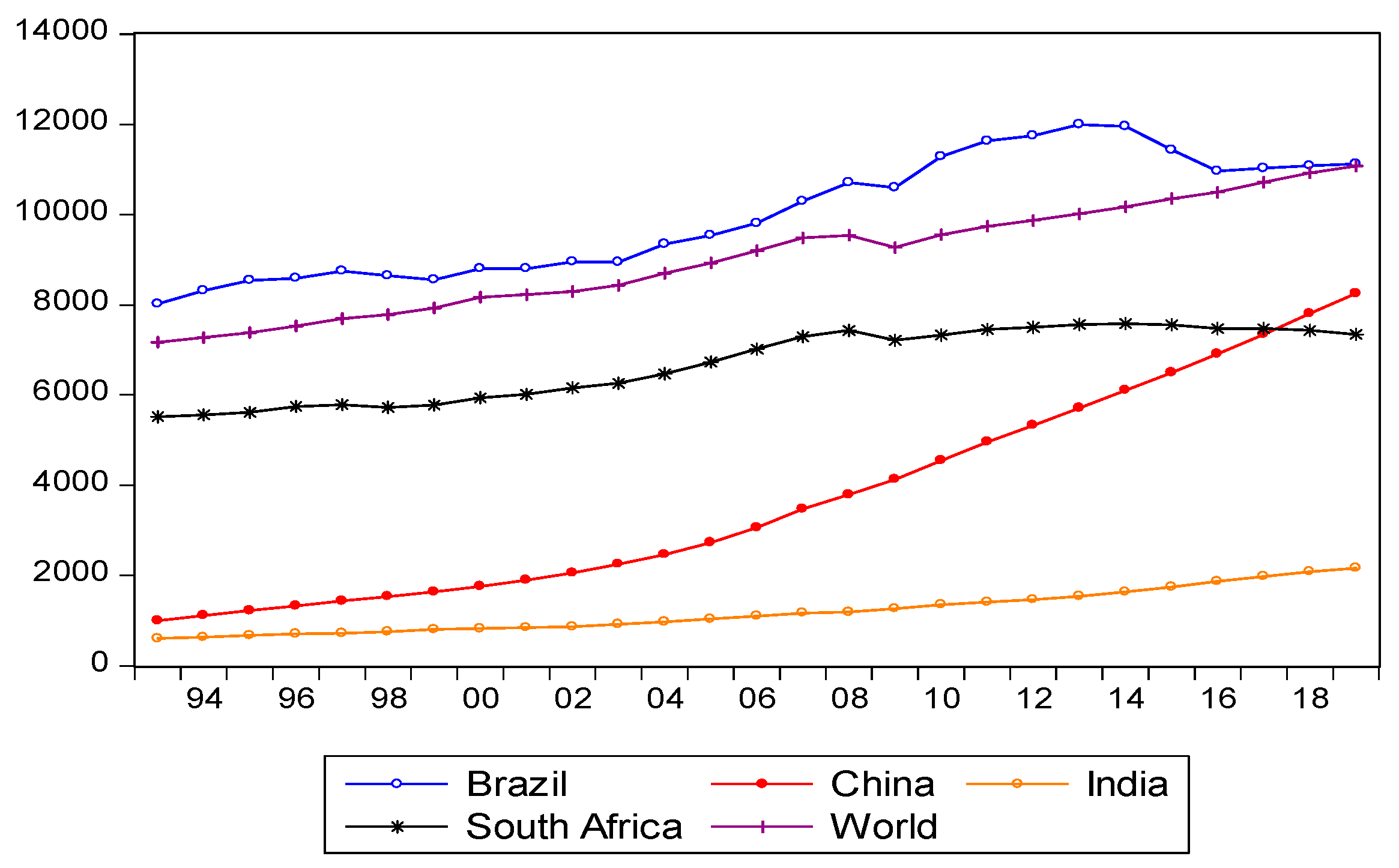
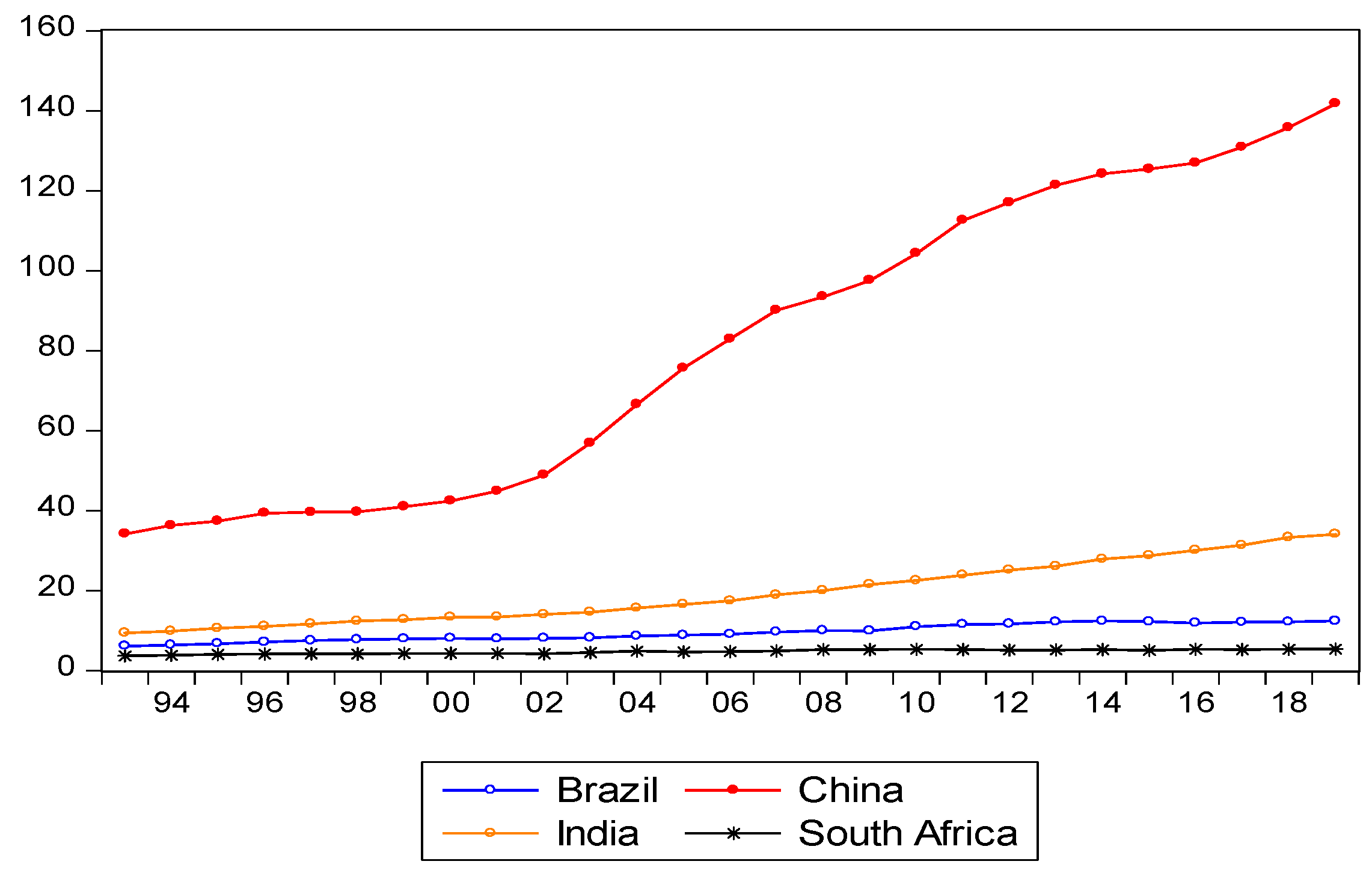
From Figure 1, it is evident that between 1993 and 2019, the GDP of the BRICS countries accounted for approximately 22% of the world’s total GDP. Although the global financial crisis occurred in 2008, various countries around the world were affected to varying degrees. Although the BRICS countries also suffered some impacts, leading to a decline in their GDP, they recovered quickly after the crisis. In the 27 years from 1993 to 2019, the country with the largest share of the global GDP of the BRICS countries was China, followed by India. Although the economic strength of the BRICS countries continues to develop, their share of the total economy of world continues to increase. However, because different countries have different developments, China and India account for a higher proportion of GDP compared to the other three countries based on this indicator. Nevertheless, the other three countries still have a lot of room for development.

Although China and India account for a relatively large total GDP and rank high among the BRICS countries, they also have large populations. Looking at their per capita GDP, they may not be the top few. According to the per capita GDP graph in Figure 2, Brazil ranks first, which is higher than the world average, while China only caught up with South Africa in second place in the last two years. India’s, a low-middle-income country, has a total population of over 1.35 billion. Its per capita GDP only slightly exceeds US$2000, the lowest among the BRICS countries. The global per capita GDP is about US$11,300 and India’s per capita is only 17% of the global per capita.

China’s per capita GDP has increased, but has not reached the global average, which is about US$9800. However, according to China’s economic growth rate and the slowdown in population growth, China’s per capita GDP is also slowly increasing, and it is likely to reach the world average level in the future. Therefore, the economic strength of the five countries can be viewed from different angles and different conclusions can be drawn.

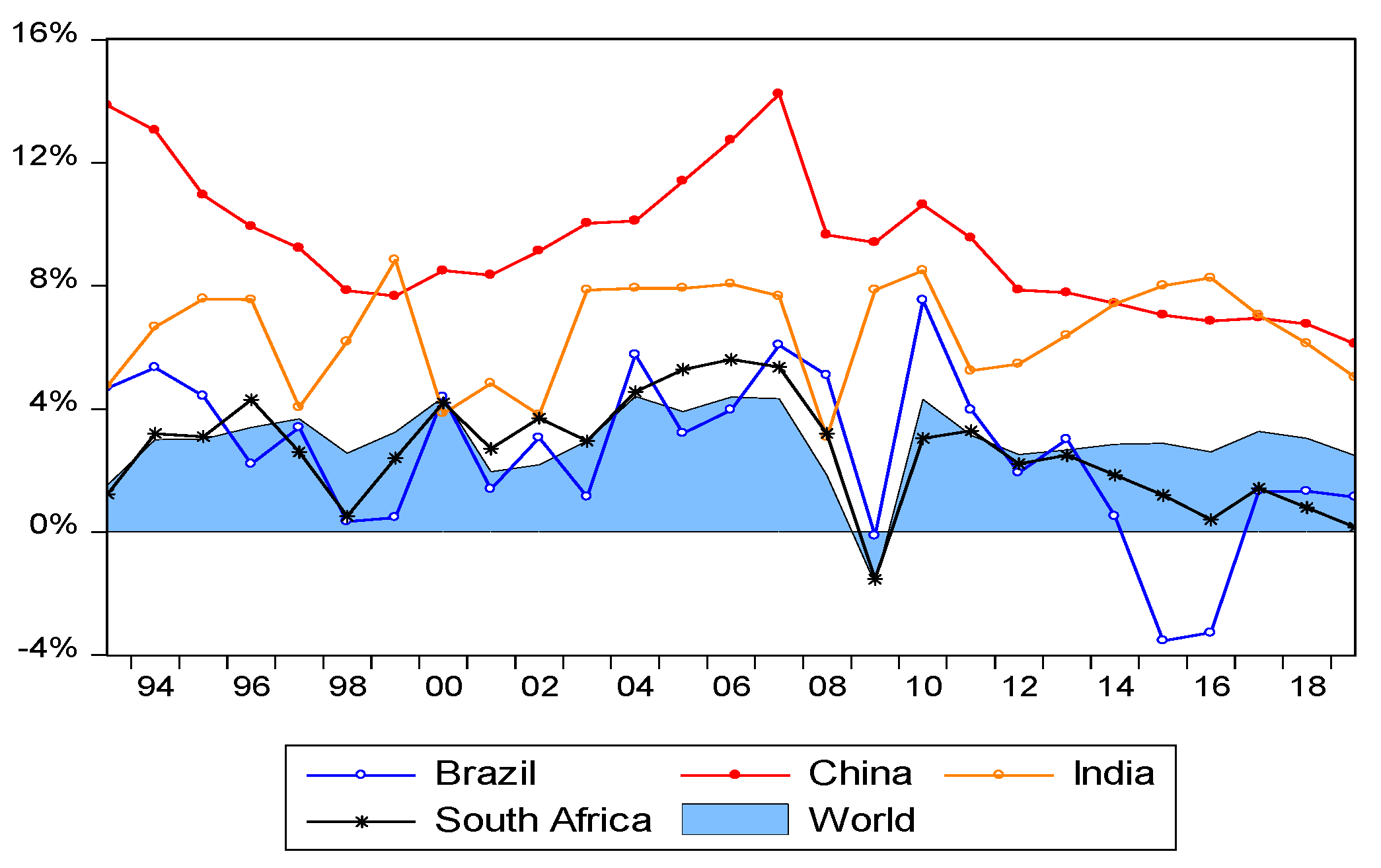
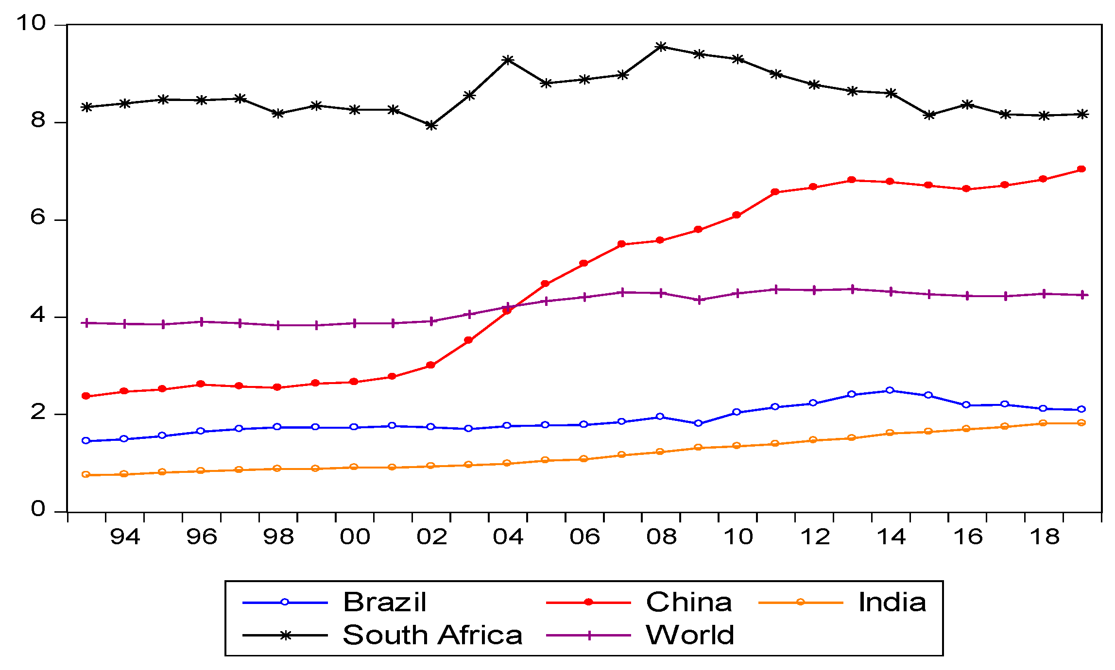
From Figure 3,

Table 1. Mean and variance of each annual growth rate index (unit: %).

	Brazil	China	India	South Africa	World
Mean	2.542479	9.369616	6.514481	2.598083	2.919798
Std. Dev.	2.625328	2.229088	1.672483	1.728913	1.221073

Note: The arithmetic average of the GDP growth rates of the four countries: 5.256165.

, it can be seen that between 1993 and 2019, the average GDP growth rate of the BRICS countries was about 4.56%, which is higher than the world average GDP growth rate; this shows that the BRICS countries have indeed developed rapidly. It is worth noting that under the circumstances of the 2008 financial crisis, although the economic growth rates of various countries have declined and many countries have even experienced negative growth, China still maintains a growth rate of 9.4%. India’s growth rate at that time was also positive.

In statistics, the average value can reflect the overall data level during the time period and the standard deviation can reflect the volatility of the data. This is expressed in Table 1 below, which combines the data from each country in Figure 1, Figure 2 and Figure 3.

The average annual GDP growth rate of China is 9.37%, which is about 6.45% higher than the world’s average GDP growth rate. After 1994, the total GDP surpassed that of several other countries and became the first. More interestingly, data from the BRICS countries show that under the global financial crisis triggered by the subprime mortgage crisis in 2008, almost all the economic growth rates of the BRICS countries were negative, but the GDP growth rate of China was still positive. Although the GDP growth rate had declined in those years, the average value remained between 6% and 7%.

India’s growth rate is relatively stable, with an average growth rate of 6.51% for more than two decades due to its large population, although its per capita GDP ranks last among the BRICS countries. However, since 2009, it has also become the second largest country in terms of GDP among the BRICS countries. The average growth rate of India’s GDP is around 6.51%, which is higher than the world’s GDP growth rate. India’s GDP growth rate has the smallest fluctuation among the BRICS countries. Under the influence of the 2008 subprime mortgage crisis, although India’s growth rate declined, it was still positive. Because of the impact of the financial crisis, India’s growth rate slowly returned to the pre-financial crisis level after 2013.

Brazil’s per capita GDP ranked first among the five countries from 1993 to 2006. From 2000 to 2010, Brazil’s economy achieved rapid development with the help of its government’s active economic policies and a better international market environment. After Lula took office as president, he introduced a series of policies conducive to the development of the Brazilian market. Under the guidance of pragmatism, Brazil ushered in a new period of prosperity and development. However, Brazil’s negative economic growth in 2015 and 2016 was due to the fact that the Brazilian government did not take timely response measures to the economic situation at the time. They adjusted public financial expenditures and reduced welfare policies that were too “developed,” leading to hyperinflation, high unemployment, and social instability. Fifteen years of Brazilian political turmoil, coupled with the Brazilian government’s fiscal austerity policy and interest rate hike measures have made the economy even worse.

South Africa is the largest economy in Africa, although the total GDP is at the bottom of the five countries. However, most of the GDP per capita ranks third. It is one of the most influential countries in Africa. South Africa is an upper middle-income economy with rich mineral resources. However, due to serious flaws in South Africa’s business model based on mining and primary manufacturing, economic growth has not increased. The data also showed that the GDP growth rate is very stable. The standard deviation is second only to India. Since South Africa joined the BRICS in 2010, it has also brought new vitality to the BRICS countries, and, at the same time, has strengthened its own vitality in participating in the cooperation between the BRICS countries. After the 2008 financial crisis, South Africa stimulated its economy by rewarding interest rates. In terms of fiscal policy, the South African government increased government budget investment, and then the GDP growth rate returned to the pre-financial crisis level the following year.

3.2. Analysis of Financial Development

3.2.1. Analysis of the General Situation of Financial Development

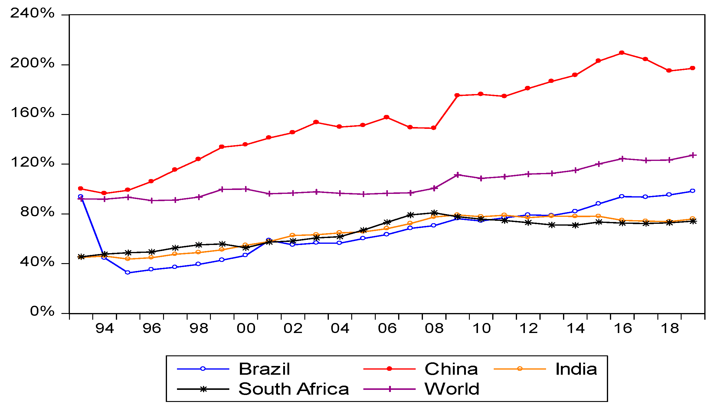
The ratio of M₂/GDP is usually used to compare the degree of financial deepening, because M₂ is the quantity of money and the stock and GDP is the gross domestic product, a flow concept. The ratio of the two measures the stock of money required per unit of output. It can also reflect a country’s macro level of development.

From Figure 4, it is clear that this indicator of the BRICS countries is increasing as a whole, indicating that the macro development trend is relatively good. However, the indicator plummeted in Brazil from 1993 to 1995 because Brazil experienced hyperinflation again at that time. The Brazilian government announced the implementation of “the Real Economic Plan” in order to subdue the hyperinflation. The plan is to ensure the relative currency in circulation in the market. Regarding stability, the government has taken measures to strictly restrict currency issuance. However, looking at the number of national indicators alone, China’s indicator is the highest, which also reflects that the scale of China’s financial development is the highest among the BRICS countries and is higher than the world average. Brazil, India, and South Africa have similar levels of this indicator.

3.2.2. Analysis of the Development of the Banking Industry

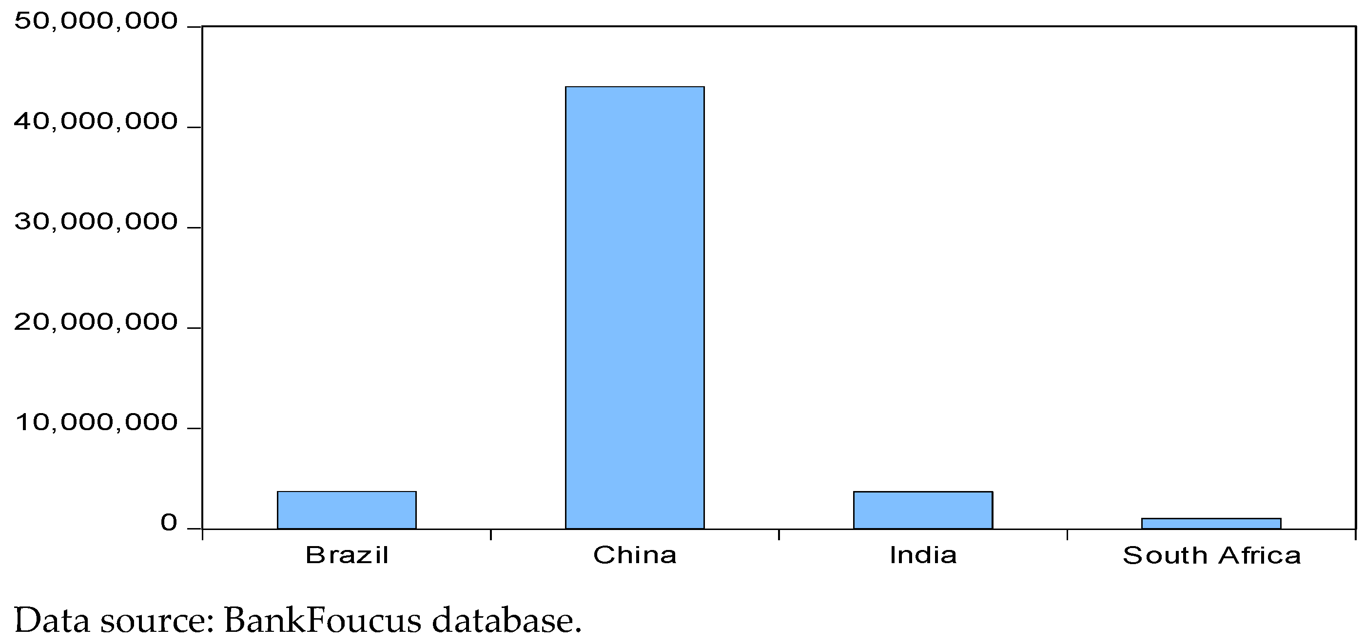
From Figure 5, it can be seen that the total asset level of the banking industry in the BRICS countries is different, and the number of banks in each country is also different. The figure also shows that the total assets of China’s banking industry are much higher than those of the other four countries, which is also largely related to China’s population and financial industry development history.

Table 2. Status of the top 1000 BRICS countries in the world Unit: USD million.

Country	Brazil	China	India	South Africa
The number of banks in the world’s top 1000 ranked by assets	10	128	24	4
The world’s highest and lowest ranking	85; 921	1; 999	58; 945	246; 702
Most assets	364,237.03	4,309,351.04	556,800.71	105,574.96
Least assets	20,480.76	18,266.93	19,786.00	29,957.61

Data source: BankFoucus database. Note: The banks in the database are ranked according to total assets. Due to their particularity, the following categories are not included in the classification: securities companies, financial companies, non-bank credit institutions, microfinance institutions, group financial companies, professional government credit institutions, bank holding, and holding companies, central banks, and multilateral government banks, liquidation and custody institutions, investment trust com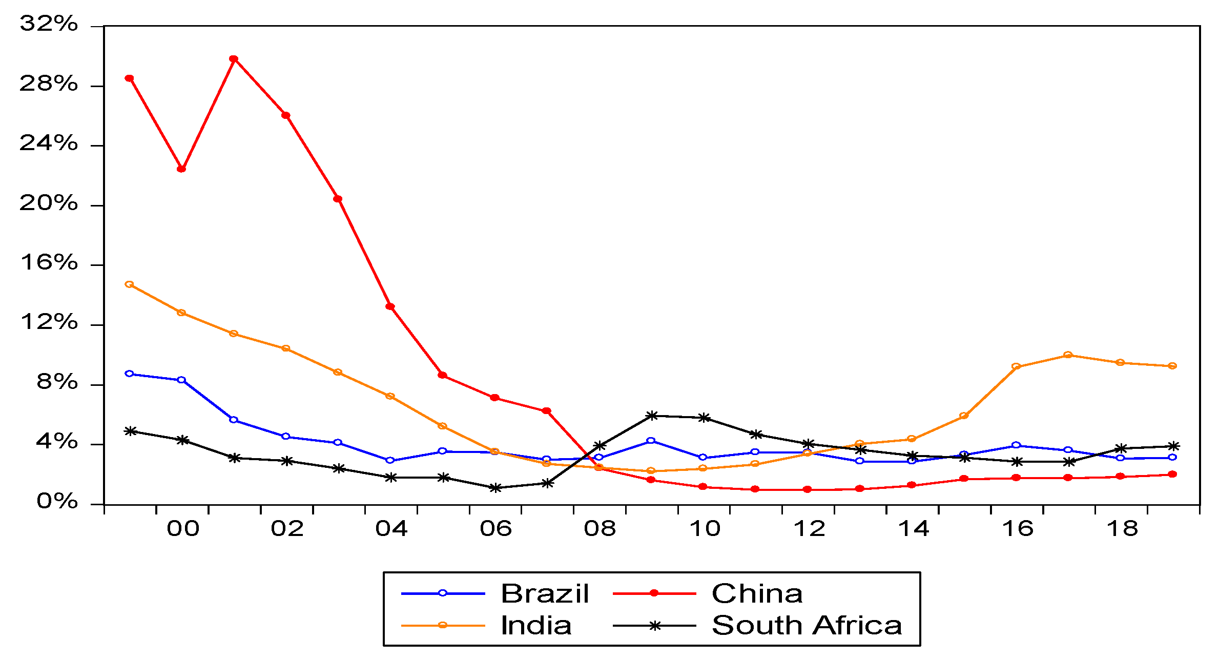panies.

indicates that there are many banking institutions in China. As seen in Figure 6, China’s non-performing loan rate has not always been low. In 1999 and 2001, the non-performing loan rate was as high as about 30%. The level has a certain relationship with the national regulatory standards at that time.

Regarding the development of the banking, the Brazilian banking system was established in the 1960s. An important feature of the Brazilian banking industry is its high degree of monopoly. Over 50% of domestic commercial institutions in Brazil are almost entirely owned by Brazil’s top eight domestic commercial banks. This has also led to the low status of the remaining small and medium-sized commercial banks. With its good response to the 2007 financial crisis, the Brazilian Commercial Bank became a safe haven. After the financial crisis, Brazilian banks actively seized opportunities to cooperate with emerging markets, and at the same time encouraged private finance. The development of institutions and the development of the domestic banking industry have entered a fast lane, which is worth learning from the BRICS.

After the reform and opening up, the banking industry of China embarked on the right track of development. A modern banking system based on central banks, policy banks, and commercial banks was gradually established. Commercial banks are divided into large state-owned commercial banks and state-level commercial banks. Commercial banks, urban commercial banks, and rural credit cooperatives formed a relatively complete banking system. At the same time, there are problems in the development of the banking industry of China. Affected by the narrowing interest rate differentials and financial disintermediation, the profitability of the banking industry has decreased; the total loan and total assets have a decreasing trend, and the mismatch of the decreasing trend has aggravated the unreasonable structure of the banking industry’s assets and liabilities. China has gradually implemented “Basel III” and the requirement for capital adequacy ratio has been further increased. This is yet another challenge for the banking industry. In short, for commercial banks, the era of rapid growth has passed. With the tightening of supervision, coupled with the shortage of funds, the pressure on profits and assets, and liabilities faced by banks, banks are forced to find new outlets. However, it depends on the situation. In the final analysis, the economic recovery of China and upgrading of consumption structure provide opportunities for the transformation and development of commercial banks.

After India’s independence, the development of its banking industry can be divided into three stages: the privatization stage, the rise of nationalization, and the development of the Indian banking industry. In the 1990s, due to the Asian financial crisis in 1997, the reform of the industrial division of the Indian banking industry went through further changes. Until this day, the Indian banking industry has maintained a hierarchical banking system. A major characteristic of the Indian banking industry is its rural banking system. India is committed to providing sufficient credit funds for rural development. Therefore, it has established targeted regional rural banks and a long-standing rural cooperative financial system. The industry proposed relevant financial policies, such as the KISAN credit card plan and the recently launched “inclusive finance.” These measures have led to certain achievements at the same time they have paid a relatively high price. South Africa’s banking system is relatively developed and complete, far ahead of other emerging economies, and not inferior to developed economies. Its banking industry has introduced a complete business system covering commercial banks, merchant banks, retail banks, insurance, and securities. Electronic banking equipment is covered all over the country and Automatic Teller Machine equipment and online banking services are popularized throughout the country.

In summary, the overall development of the banking industry in the BRICS countries is relatively fast, but due to their own development history, their development is facing different difficulties. This is a problem that all countries need to solve.

3.2.3. Analysis of the Development of the Securities Market

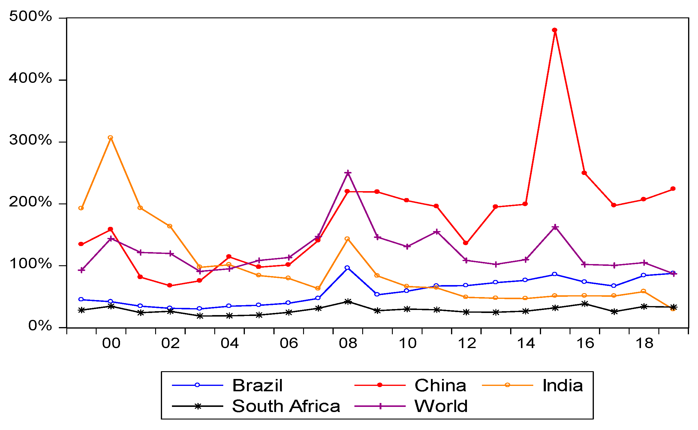
Stock transaction turnover rate refers to the total amount of stock transactions within a certain period divided by the average market value of listed companies during that period. In Figure 7, from 2006 to 2007, the stock market was in good condition because of the bull market globally, and almost all global stock markets were rising. In 2008, the bear market was accompanied by the emergence of the financial crisis, and global stock markets fell. After the bull market in China in 2009, the stock market became volatile for five consecutive years. As the stock market had a certain linkage effect, during China’s bull market in 2015, the stock market turnover rate of other countries in the world increased accordingly. As of 2019, the stock turnover rate of the BRICS countries is higher than the world average, which shows that the stock markets of the BRICS countries are relatively active, of which China has the highest proportion, reflecting that the stock market is very active.

Because the development of the country is different, the development of the securities market in each country is also different. The development of the Brazilian securities industry can be traced back to the Brazilian Stock Exchange established in 1890. In the 1970s, in order to stimulate the development of the domestic securities market, Brazil introduced a large number of foreign investors, and its investment scale once reached 25%. However, after the financial crisis, foreign investors withdrew one after another, thereby causing violent fluctuations in the Brazilian securities market, and affected the country’s economic development. It can be seen that the economic development of a country cannot rely too much on foreign investment, and the BRICS countries should use this as a warning. Brazil Futures Exchange and Sao Paulo Stock Exchange underwent shareholding reforms in 2007 and merged into Brazil Stock Exchange. The newly established exchange has a wealth of trading varieties and adopts electronic trading methods. As of 2011, it has become the world’s twelfth largest fund-raising market with huge development potential.

The development of the securities industry of China began with the reform and opening up in 1978. The Shenzhen Stock Exchange and Shanghai Stock Exchange, established on 1 and 18 December 1990, are milestones in the development of China’s securities industry. As of May 2018, the number of companies listed on the Shenzhen Stock Exchange has reached 2112, and the total market value of A-shares has reached 335.256 billion US dollar. The number of companies listed on the Shanghai Stock Exchange has continued to grow. The number of listed companies on the Shanghai Stock Exchange reached 1423, and the total market value of A-shares reached 4730.259 billion US dollar. Yuan, far ahead of other BRICS countries: In the field of stock trading, the small and medium board of directors established in 2004 and the ChiNext board of directors established in 2009 facilitated the financing of small-sized and medium-sized enterprises and innovative companies. As of May 2018, there are 911 listed companies on the small-sized and medium-sized board and 725 listed companies on the GEM, which are indistinguishable from the mainboard market: as far as the types of transactions are concerned, not only stocks can be traded, but also funds, bonds, convertible bonds, ETFs, and warrants.

In terms of trading scope, the Shanghai–Hong Kong Stock Connect opened in 2014 and the Shenzhen–Hong Kong Stock Connect opened in 2016 and have expanded the investment scope of Chinese investors and provided international choices. At the same time, in recent years, with the increase in national income, the enthusiasm of the whole society for securities investment has gradually increased. At the same time, the regulatory agencies have taken more effective measures to regulate their development in accordance with the changes in reality.

However, it is important to note the issues affecting the development of China’s securities industry. Securities companies have a relatively simple way of making profits, mainly relying on traditional businesses such as securities brokerage and self-operation of securities. Compared with the securities industry in developed economies, the scale of China’s securities industry is small. The investment variety is too small and diversified services cannot be realized. Thus, it cannot effectively diversify risks, nor attract capital, and expand profits. With the opening of the market, the influx of international institutions, competition, and insufficient innovation capabilities, it is difficult to keep up with the market. In some gray areas, such as private equity, insufficient supervision and risk can be easily induced, stockholders are unable to make rational investments, and the phenomenon of following the trend is obvious. These problems are restricting the further development of China’s securities industry.

India is the first country in Asia to have a stock exchange. Its first stock exchange, the Bombay Stock Exchange, was established in 1875. As of 2018, the number of listed companies reached 5648, and the number of listed companies reached 5985 between 2016 and 2017 (Data sources: NSE India (National Stock Exchange of India Ltd.; https://www.nseindia.com/ (assessed on 18 June 2021)). The National Stock Exchange of India was established in November 1992 and is another major stock exchange in India. As of May 2018, more than 1300 stocks were traded, with a trading volume of 21.468 billion US dollar and a market capitalization of 33.101 billion US dollar, making it India’s largest stock exchange and the world’s third highest trading volume. It is evident that the Indian securities industry has impressive strength and huge development potential.

The South African Stock Market was established in 1887. The stock exchange was the Johannesburg Stock Exchange. At the beginning of the establishment, the exchange was mainly to raise funds for the development of gold mines. With the development, financing models and trading products gradually changed from mining stocks to financial stocks. As the largest equity market on the African continent, the market value of companies listed on the Fort Johannesburg Stock Exchange accounted for more than 70% of the market value of listed companies in Africa.

From the foregoing, it is clear that there are still gaps in the development of the securities industry in the BRICS countries; as their characteristics differ, so do their advantages, shortcomings, and development potential.

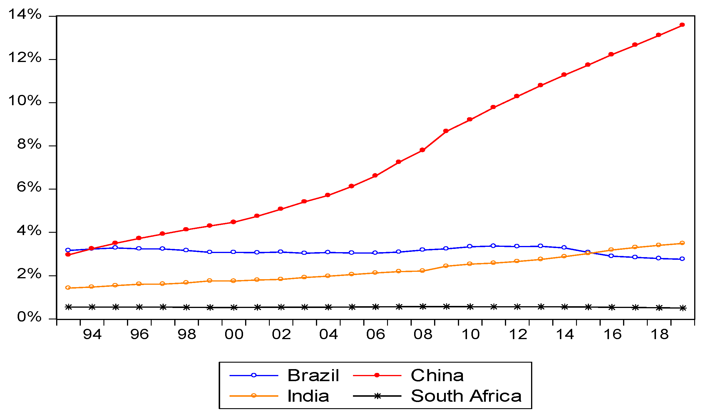
3.3. Analysis of CO₂ Emissions

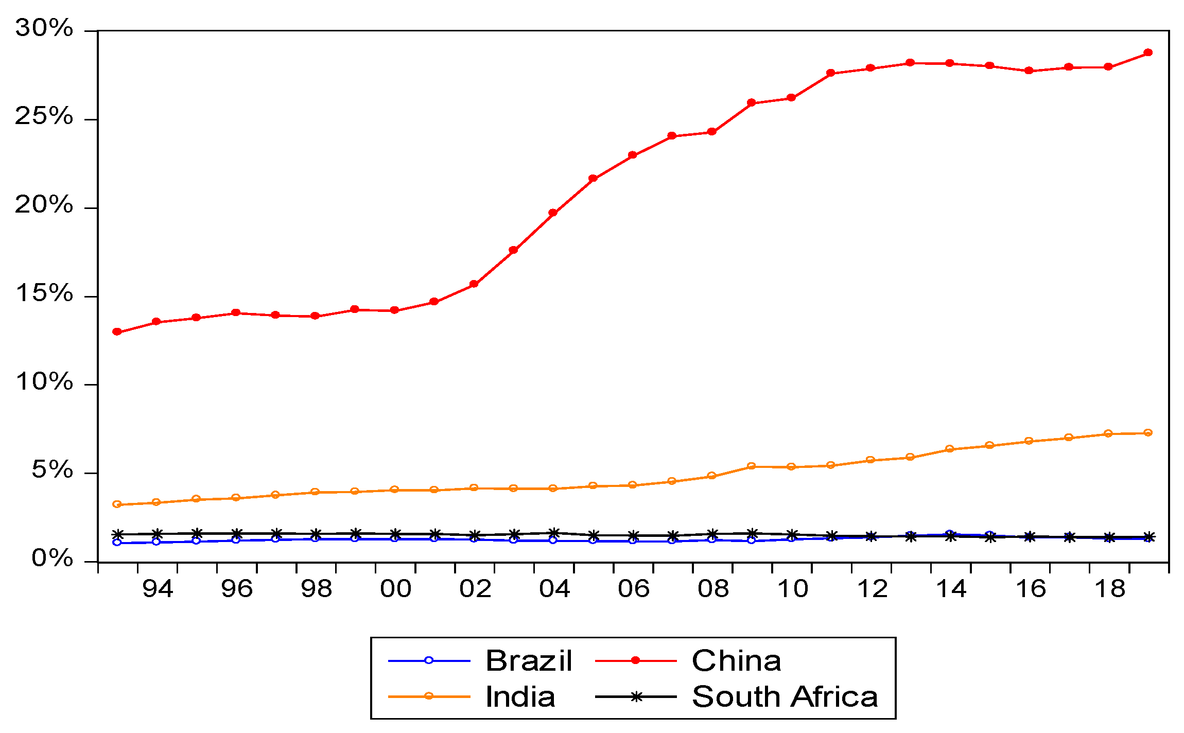
Economic development has brought about a large amount of waste discharge. CO₂ emissions are usually used to measure the world’s emission indicators, especially the “Kyoto Protocol” passed in Kyoto, Japan, in December 1997, which has aroused the global fanaticism about greenhouse gases (mainly CO₂). First of all, it can be seen, from Figure 8, that from 1993 to 2019, the proportion of the BRICS countries in world CO₂ emissions increased year by year in China and India, while the changes in Brazil and South Africa were not particularly obvious. China, in particular, accounted for a relatively high proportion of CO₂ emissions in 1993. It has continued to strive for development in the course of exploration. The level of industrial development has gradually increased, and CO₂ emissions have also increased accordingly. By 2019, China’s total CO₂ emissions accounted for 28.76% of the world’s total CO₂ emissions, ranking first among the four BRICS countries. Although India’s global CO₂ emissions are much lower than China’s, it is likely to slowly increase in due course. India’s total CO₂ emissions worldwide accounted for 7.25% of the world’s total, ranking second among the BRICS countries. Compared to the other three countries, the CO₂ emissions of Brazil and South Africa are relatively small and there have been no significant changes. By 2019, South Africa’s total CO₂ emissions accounted for 1.40% of the world’s total CO₂ emissions, ranking fourth among the BRICS countries and Brazil’s total CO₂ emissions accounted for 1.29% of the world’s total emissions, ranking fifth among the BRICS countries.

The CO₂ emissions and energy use are also inextricably linked. As shown in Figure 9, the energy consumption performance trend of the BRICS countries can be divided into two different stages according to time, the slow growth interval from 1993 to 2002 and 2004, and the range in which consumption has risen rapidly after the year. Among them, the fastest growing is China, which is also related to China’s rapid development after the 21st century. The main reason for the growth is the rapid growth of China’s energy consumption, which is consistent with the rapid development of its economy. India’s development is at a relatively steady pace and energy consumption is also relatively steady. Brazil and South Africa have slow growth in energy consumption, which is similar to the growth rate of their total CO₂ emissions.

Figure 10 shows that South Africa’s per capita carbon emissions are very high, and it has the highest per capita CO₂ emissions. South Africa has the second highest per capita CO₂ emissions account. It is rich in mineral resources; since the end of international sanctions in the early 1990s and the establishment of the new South Africa in 1994, the country’s economy has been in a state of steady growth.

China ranks third in CO₂ emissions per capita. This is in line with the fluctuations in the overall increase in CO₂ emissions per capita. Although China’s per capita carbon dioxide emissions in the 1990s were lower than the world average, China’s rapid development since the beginning of the 21st century after its accession to the World Trade Organization, led to the development of its manufacturing industries, resulting in rapid increases in its CO₂ emissions. With China’s rapid development in the 21st century, the rise of industry and manufacturing required the support of large amounts of energy. As coal became the main energy fuel, carbon emissions increased quickly. Due to China’s large population, even if the per capita CO₂ emissions are very low, the total amount would still be very large. Therefore, in recent years, China has continuously adopted energy-saving and emission-reduction measures to contribute to environmental protection.

Brazil and India ranked fourth and fifth, respectively. Brazil and India are emerging economies and their economic growth rates are relatively slow. Thus, the two countries are constantly exploring suitable development paths and striving to improve the level of development. The development process has also been accompanied by the process of urbanization and industrialization, thus, there is a large demand for energy and resources, energy consumption, and CO₂ emissions. Therefore, the pressure is greater; the impact of the two countries on the environment is also worth noting.

CO₂ emissions of the BRICS countries have always been an issue of concern. Countries are constantly cooperating to save energy and reduce emissions to contribute to environmental protection. Through cooperation, exchanges, and a mutually beneficial, win-win strategic policy, there will be an improvement in production, science and technology, innovative technology, optimization of energy structures, and regional economic integration, resulting in a resource-saving and environment-friendly society.

4. Methodology of Research

4.1. Data and Hypothesis

4.1.1. Data and Variables

This paper used data on GDP, financial development, and CO₂ emissions from the BRICS countries. Financial development and GDP data were adjusted based on 1980s prices, and, thus, the 1980 deflator was used. CO₂ emissions were calculated based on the per capita CO₂ emissions of the BRICS countries. Due to the requirements of the model, the variable were a stationary time-series of I(0) or I(1), to prevent the occurrence of false regression. In the unit root test, where the data was displayed as I(2), the data was discarded. The data of Russian wasn’t I(0) and I(1) in unit root test, so it was not used in this paper. The per capita CO₂ emissions were divided by metric tons to calculate per capita CO₂ emissions in this paper. Financial development and gross national product data were retrieved from the World Bank database. CO₂ emissions data was taken from the public database of British Petroleum. The selected data range was from 1978 to 2019 and we use Metlab’s software package to perform quantile on quantile regression test.

4.1.2. Hypotheses

This paper has the following hypotheses:

Hypothesis 1 (H1).

Financial development positively affects CO₂ emissions in BRICS.

Financial development has an effect on CO₂ emissions. The increase in manufacturing activities in the financial sector may lead to industrial pollution and higher CO₂ emissions. This situation is usually seen in emerging markets like China [47] and India [48,49].

Hypothesis 2 (H2).

Financial development causes a reduction of CO₂ emissions in BRICS.

Financial development reduces CO₂ emissions due to the development of new technologies and the implementation of environmental regulations by increasing income and capitalization on foreign direct investment. To support this assertion, case studies were drawn from the BRICS countries [50], that is, China [51,52,53] and Brazil [54].

4.2. Quantile on Quantile Regression Method

The most commonly used regression in statistics is ordinary least squares (OLS) estimation, but when encountering abnormal value in the data, the OLS estimation will be greatly disturbed and, thus, not stable enough; in the heteroscedastic model, the OLS method is even the facts may be seriously misinterpreted. The model estimated by the OLS method reflects the influence of the change of the independent variable $X$ on the average value of the dependent variable $Y$, and does not reflect the core of our concern. Quantile regression (QR) is a regression analysis method that estimates the parameters of the model by minimizing the weighted sum of the absolute values of the residuals. As a supplement and extension of the traditional regression method (OLS), QR makes up for the shortcomings of the OLS method in the presence of heteroscedasticity in the model, and the robustness of the quantile can ensure the robustness of QR, which makes up for the shortcomings of the OLS method not robust enough to handle abnormal data.

QR focuses on the conditional quantile function, and the quantile can take any quantile of the distribution, so the fit obtained by QR is a series of fits, which can not only reflect the distribution of the center position the situation (that is, the median) can also reflect the distribution of non-central locations (the tail of the dependent variable distribution). The quantile-on-quantile regression (QQR) is an empirical study of how the quantiles appearing from one variable affect the conditional quantiles of another variable. As mentioned earlier, QQR can provide richer information than alternative estimation techniques such as OLS or traditional QR. The QQR is used partial linear regression techniques to check the partial influence of a specific quantile of the independent variable on the dependent variable. The main purpose of this partial linear regression technique is to determine the partial linear regression around the neighborhood of each data point in the sample, and to provide a higher weight to the direct neighbor of each data point.

4.2.1. Fourier Toda-Yamamoto’s Causality Test

The Fourier Toda-Yamamoto quantile model was used in this paper. In order to solve the problem of structural changes in causality, dummy variables from Cai et al. [55], Lin et al. [56], and Goh et al. [57] were added to the model. However, dummy variables can only allow changes that occur during a certain period. There may be some dramatic changes and structural changes that occur, which dummy variables will not be able to capture. Therefore, the Fourier approximation was used to solve the unknown multiple structural breaks problem ([58,59]).

The Fourier functions was used in combination with $QT-Y$, which is the $QFT-Y\left(p+d\right)$ model. It used the Toda-Yamamoto component regression model of Fourier functions. The Fourier function expansion d (t) is defined as follows:

$$d\left(t\right)=m_1\sin \left(\frac{2\pi wt}{T}\right)+m_2\mathrm{con}\left(\frac{2\pi wt}{T}\right)$$

(1)

where $w$ is the frequency, $T$ is the number of observations, t is the trend term, respectively, and $m_1$ and $m_2$ are the coefficients of sin(·) and con(·), respectively. Using the BFGC-Q method to test Granger’s null hypothesis of non-causality, a two-step procedure was designed:

First, it was necessary to control a smooth break. Under deterministic conditions, the Fourier expansion of $d\left(t\right)$ is contained in the following Granger causality equation:

$$Y_t=v_0+{\mathrm{m}}_1\sin \left(\frac{2\pi wt}{T}\right)+m_2\cos \left(\frac{2\pi wt}{T}\right)+{{\displaystyle \sum }}_{i=1}^{p+h}{\theta }_i{Y}_{t-i}+{{\displaystyle \sum }}_{j=1}^n{{\displaystyle \sum }}_{i=1}^{p+h}{\vartheta }_{j,i}{X}_{j,t-i}+{\epsilon }_t$$

(2)

where, $Y$ and $X$ are the dependent variables and the independent variable, $p$ is the lag length, $h$ is the maximum degree of integration of the variable, and n is the number of common variables. The coefficients $m_1$ and $m_2$ of sin(·) and cos(·) in the Fourier function of the $F$ test were used to confirm whether there were structural changes in this study. Where the test result rejected the H₀ null hypothesis, there were structural changes, and then the structural change model was used. Otherwise, the non-structured model was used.

The hypotheses of the structural change test are:

The null hypothesis $H_0: m{ }_1=m_2=0$ (without structural changes).

The alternative hypothesis $H_1: m{ }_1\ne 0 \mathrm{or} m_2\ne 0$ (with structural changes).

Second, the null hypothesis of Granger’s non-causal relationship was used to estimate the regression model through the QR method of Equation (3), allowing the testing of the null hypothesis of Granger’s non-causal relationship between X and Y at different quantiles, where Z was the regression model of Equation (3). The matrix of all cointegration variables in Equation (3) was used to find the minimum number of lagging periods and the optimal frequency.

$$\begin{gathered} Q_{Y_t}\left(\tau |\mathrm{Z}\right)=m_0\left(\tau \right)+m_1\left(\tau \right)\sin \left(\frac{2\pi w^{*}t}{T}\right)+m_2\left(\tau \right)\cos \left(\frac{2\pi w^{*}t}{T}\right)+{{\displaystyle \sum }}_{i=1}^{p^{*}+h}{\theta }_i\left(\tau \right)Y_{t-i}+ \\ {{\displaystyle \sum }}_{i=1}^{p^{*}+h}{\vartheta }_{j,i}\left(\tau \right)X_{j,t-i}+{\epsilon }_t \end{gathered}$$

(3)

The selection of the most suitable lag period in the model was through the test of the null hypothesis, and according to the Akaike Information Criterion (AIC) criterion proposed by Akaike [60], the optimal lag period $p^{*}$ of the model was selected. Similarly, for $k$ in the Fourier function, after setting w = [0.1, 0.2,…, 5], the best $w^{*}$ was also selected according to the AIC criterion. The hypothesis test of the model in this study was as follows: If the $H_0$ null hypothesis is rejected, it means that there is a significant Granger causality between the independent variable and the strain at this quantile:

$$H_0: {\widehat{\vartheta }}_{j, 1}\left(\tau \right)={\widehat{\vartheta }}_{j,2}\left(\tau \right)=\dots ={\widehat{\vartheta }}_{j,p^{*}}\left(\tau \right)=0, \forall \tau \in \left(0, 1\right)$$

(4)

The null hypothesis $H_0: {\widehat{\vartheta }}_{j, 1}\left(\tau \right)=0$ (there is no causal relationship).

The alternative hypothesis $H_1: {\widehat{\vartheta }}_{j, 1}\left(\tau \right)$ ≠ 0 (there is a causal relationship).

This model used the Wald test statistics subject to Chi-square distribution as follows:

$$\mathrm{Wald}=[\mathrm{T}({\left({\widehat{\vartheta }}_j\left(\tau \right)\right)}^{\prime }{( \hat{\mathsf{\Omega }}\left(\tau \right))}^{-1}\left({\widehat{\vartheta }}_j\left(\tau \right)\right))]/\tau (1-\tau )$$

(5)

where ${\widehat{\vartheta }}_j\left(\tau \right)$ parameter index matrix and $\hat{\mathsf{\Omega }}\left(\tau \right)$ is the variance-covariance matrix of ${\widehat{\vartheta }}_j\left(\tau \right)$ infinite model. In addition, in order to improve the verification ability of small samples, the study used Hatemi-J and Uddin’s [61] research to point out that due to the autoregressive conditional heteroscedasticity (ARCH) effect in the data, they are usually abnormally distributed, and there is a possibility of significant deviation from the asymptotic distribution. The bootstrapping simulation technique was used to perform 10,000 repeated simulation calculations to find the 10%, 5%, and 1% critical values.

4.2.2. Cointegration Test

This paper adopted Bayer and Hanck’s [62] proposal to introduce a new cointegration method called joint cointegration method for research. The cointegration methods of Engle and Granger (EG) [63], Johansen (JOH) [64], Boswijk (BO) [65], and Banerjee et al. (BDM) [66] were combined to obtain a comprehensive cointegration result. The Fisher equation [67] was then used to calculate the F statistic to obtain more conclusive and reliable empirical results. The Fisher equation used to calculate the Bayer and Hanck cointegration equation was:

$$\begin{gathered} EG-JOH=-2\left[\ln \left(P_{EG}\right)+\ln \left(P_{JOH}\right)\right] \\ EG-JOH-BO-BDM=-2\left[\ln \left(P_{EG}\right)+\ln \left(P_{JOH}\right)+\ln \left(P_{BO}\right)+\ln \left(P_{BDM}\right)\right] \end{gathered}$$

The $P$ values of different individual cointegration tests include $P_{EG}, P_{JOH},$ $P_{BO}, P_{BDM}$. If the estimated Fisher statistic exceeds the critical value provided by Bayer and Hanck [62], the null hypothesis will be rejected, so there is cointegration. In this paper, we adopted Bayer and Hank, joint cointegration to test whether there is a cointegration relationship among the CO₂ emissions, financial development and GDP of the BRICS countries.

4.2.3. Quantile on Quantile Regression Approach

This study proposed a quantile on quantile (QQR) test weighted median weight regression method, suggested by Sim and Zhou [68], to test the comprehensive relationship between CO₂ emissions, financial development, and economic growth in the BRICS countries.

$$C{O}_2{}_t={\beta }^{\theta }\left(F{D}_t\right)+W\left(C{O}_2{}_{t-1} \right)+\gamma \left(\mathit{GDP}\right)+u_t^{\theta }$$

(6)

Equation (6) is a local linear equation, so in Equation (1), in the non-parametric QR model, $\theta$ has the conditional distribution quantile of CO₂ emissions, $\mathit{GDP}$ is the control variable, and $u_t^{\theta }$ is the error term of the conditional component. The relationship between the $\theta$^th quantile’s CO₂ emissions and the $\theta$^th quantile’s financial development was analyzed, followed by the τ^th quantile’s CO₂ emissions and the $\tau$th quantile’s financial development, to $GD{P}^{\tau }$. The area around τ adopts a local linear regression. Because ${\beta }^{\theta }(*)$ is unknown, this function used the first-order Taylor expansion in the quantile $F{D}^{\tau }$, the equation was used as follows (7):

$${\beta }^{\theta }\left(F{D}_t\right)={\beta }^{\theta }\left(F{D}^{\tau }\right)+{\beta }^{{\theta }^{\prime }}\left(F{D}^{\tau }\right)\left(F{D}_t-F{D}^{\tau }\right)$$

(7)

where ${\beta }^{{\theta }^{\prime }}$ is the partial derivative of ${\beta }^{\theta }\left(F{D}_t\right)$, which is also called the marginal effect and is similar in interpretation to the slope coefficient in the linear regression model. Furthermore, because $\theta$ and $F{D}_t$ are functions of ${\beta }^{\theta }\left(F{D}^{\tau }\right)$ and ${\beta }^{{\theta }^{\prime }}\left(F{D}^{\tau }\right)$, and $\tau$ is a function of $F{D}_t$, $\theta$ and $\tau$ are functions of ${\beta }^{\theta }\left(F{D}^{\tau }\right)$ and ${\beta }^{{\theta }^{\prime }}\left(F{D}^{\tau }\right)$, so ${\beta }^{\theta }\left(F{D}^{\tau }\right)$ and ${\beta }^{{\theta }^{\prime }}\left(F{D}^{\tau }\right)$ are individually rewritten as ${\beta }_0\left(\theta ,\tau \right)$ and ${\beta }_1\left(\theta ,\tau \right)$, so program (7) can be rewritten as Equation (8):

$${\beta }^{\theta }\left(F{D}_t\right)\approx {\beta }_0\left(\theta ,\tau \right)+{\beta }_1\left(\theta ,\tau \right)\left(F{D}_t-F{D}^{\tau }\right)$$

(8)

Placing Equation (8) into Equation (6), will result in Equation (9):

$$C{O}_2{}_t={\beta }_0\left(\theta ,\tau \right)+{\beta }_1\left(\theta ,\tau \right)\left(F{D}_t-F{D}^{\tau }\right)+W\left(C{O}_2{}_{t-1}\right)+\gamma \left(GDP\right)+u_t^{\theta }$$

(9)

In Equation (9), $C{O}_2{}_t={\beta }_0\left(\theta ,\tau \right)+{\beta }_1\left(\theta ,\tau \right)\left(F{D}_t-F{D}^{\tau }\right)+u_t^{\theta }$, because there will be no linear relationship between the components in the quantile. Therefore, because of the interconnection between economic uncertainty and the respective distribution of $GDP$, the overall structure of economic uncertainty and $GDP$ was estimated. The asymmetric causal effect proposed by Granger and Yoon [69] and Hatemi-J [70] on $F{D}_t$ was also used to test the positive and negative impact using the following Equation (10):

$$F{D}_t^{+}={{\displaystyle \sum }}_{i=1}^t{\epsilon }_{1t}^{+}, F{D}_t^{-}={{\displaystyle \sum }}_{i=1}^t{\epsilon }_{1t}^{-}, \mathrm{and} C{O}_2{}_t^{+}={{\displaystyle \sum }}_{i=1}^t{\epsilon }_{2t}^{+}, C{O}_2{}_t^{-}={{\displaystyle \sum }}_{i=1}^t{\epsilon }_{2t}^{-}$$

(10)

Equation (10) and $F{D}_t$ were combined, as in Equation (11):

$$F{D}_t=F{D}_t^{+}+F{D}_t^{-}={\displaystyle \sum }{\epsilon }_{FD}^{+}+{\displaystyle \sum }{\epsilon }_{FD}^{-}$$

(11)

The estimation in Equation (11) requires individual estimated values ${\widehat{FD}}_t$ and ${\widehat{FD}}^{\tau }$ to replace $F{D}_t$ and $F{D}^{\tau }$ to obtain local linear regression of parameters $b_0$ and $b_1$, by solving the following minimization problems, the estimated values of ${\beta }_0$ and ${\beta }_1$ are as follows:

$$\underset{b_{0,}{b}_1}{\min }{{\displaystyle \sum }}_{i=1}^n{\rho }_{\theta }\left[F{D}_t-b_0-b_1\left({\widehat{FD}}_t-{\widehat{FD}}^{\tau }\right)+W\left({\mathrm{CO}}_2{}_{t-1}\right)\right]\ast K\left(\frac{F_n\left({\widehat{FD}}_t-\tau \right)}{h}\right)$$

(12)

Finally, in the application of non-parametric analysis, the Gaussian kernel was used in the calculation. The observation values near the weighted $F{D}^{\tau }$ were symmetrical around zero and the far observation values were assigned low weights, that is, these weights were compared with ${\widehat{FD}}_t.$ The distance between the actual distribution function of $\tau$ is inversely proportional and $h$ is the bandwidth. The bandwidth determines the size of the neighborhood around the target point. The choice of bandwidth is very important in determining the smoothness of the bandwidth control result estimation. The larger the bandwidth is, the larger the potential estimation deviation; the smaller the bandwidth is, the larger the estimation variance. Therefore, it is necessary to choose a bandwidth that achieves a balance between deviation and variance. This study used the bandwidth parameter $h=0.05$ as suggested by Sim and Zhou [68].

The QQR method can be regarded as a method of decomposing the estimation of the standard QR model, so as to obtain the specific estimated value of different quantile explanatory variables. In the framework of this research, the QR model is based on the regression of $\theta$th quantile economic growth and financial development on $C{O}_2{}_t$. Therefore, the QR parameters are only guided by $\theta$. However, as mentioned earlier, the QQR analysis will return to the $\tau$/GDP quantile on the $\theta$/CO₂ quantile and its parameters will be jointly guided by $\theta$ and $\tau$. Therefore, compared to the QR model, the QQR method contains more detailed information about the relationship between financial development and CO₂ because the QQR method suggests that this relationship may be different from the quantile of economic growth. Considering the inherent decomposition characteristics of the QQR method, the estimated value of QQR can also be used to restore the estimated value of standard QR. Specifically, through $\tau$, the average QQR parameter could only be determined by the generation of $\theta$ QR parameters. For example, the slope coefficient of the QR model was obtained in a way that measures the influence of $F{D}_t$ on the distribution of $C{O}_2{}_t$. This can be expressed by ${\gamma }_1\left(\theta \right)$, as shown in the following procedure (9):

$${\gamma }_1\left(\mathsf{\theta }\right)\equiv {\overline{\widehat{\beta }}}_1\left(\theta \right)=\frac{1}{S}{{\displaystyle \sum }}_{\tau }{\widehat{\beta }}_1\left(\mathsf{\theta },\tau \right)$$

(13)

where S is the number of quantile considered $\tau =\left[0.05,0.10...,0.95\right]$. A simple way to test the effectiveness of the QQR method is to combine the estimated component regression parameters with $\tau$ and compare the average QQR parameters. As shown in the table below, regardless of which quantile is considered, the average QQR estimate of the slope coefficient is very similar to the QR estimate of all countries.

4.3. Empirical Result Analysis

Table 3. Statistics Description.

	BRAZIL_CO2	CHINA_CO2	INDIA_CO2	SAFRCA_CO2	BRAZI_FD	CHINA_FD	INDIA_FD	SAFRCA_FD
Mean	305,760	479,782	110,651	375,250	52.5721	117.47	55.208	60.509
Median	312,289	340,518	936,221	372,042	56.3320	123.90	48.901	56.454
Maximum	533,530	102,919	2,480,400	503,112	111.3253	207.67	79.075	80.799
Minimum	162,961	131,031	279,051	199,950	10.0829	24.185	29.481	45.500
Std. Dev.	111,623	319,501	704,502	86040.	29.925	57.831	16.735	10.543
Skewness	0.3835	0.6523	0.6562	−0.2897	0.0544	−0.0704	0.2009	0.4952
Kurtosis	1.9166	1.8349	2.1552	2.1396	1.7941	1.6691	1.4686	1.7173
Jarque-Bera	3.1574	5.4821 *	4.3646	1.9281	2.6265	3.2091	4.4909	4.705 *
Probability	0.2062	0.0645	0.1127	0.3813	0.2689	0.2009	0.1058	0.0951
	BRAZI_GDP		CHINA_GDP		INDIA_GDP		SAFRCA_GDP
Mean	1.57 × 1012		3.34 × 1012		1.06 × 1012		2.84 × 1011
Median	1.47 × 1012		1.91 × 1012		7.73 × 1011		2.50 × 1011
Maximum	2.42 × 1012		1.15 × 1013		2.96 × 1012		4.30 × 1011
Minimum	8.38 × 1011		2.64 × 1011		2.76 × 1011		1.68 × 1011
Std. Dev.	5.17 × 1011		3.36 × 1012		7.77 × 1011		8.63 × 1010
Skewness	0.3333		1.0517		0.9935		0.4821
Kurtosis	1.7219		2.8261		2.8670		1.7205
Jarque-Bera	3.7227		7.9821 **		7.1068 **		4.5990
Probability	0.1554		0.0184		0.0286		0.1003

Note: ** and * indicate that the null hypothesis is at the significance level of 5%, and 10%.

shows that, except for South Africa’s CO₂ data and China’s financial development data, all other data show a right-skewed stance. Except for the economic growth of China and India, other data are in line with normal distribution. In general, most of the data show a normal distribution with a right-skewed stance. Figure 11 shows that Brazil’s financial development data experienced great fluctuations in the 1990s. Because of the federal public deficit, Brazil mainly relies on the issuance of additional currency and federal short-term bonds to make up for it. However, the issuance of this currency is not a purely monetary act based on the development of production, which leads to rising prices and rising inflation. In order to stabilize the economy, the Brazilian government promulgated many anti-inflation plans such as the “Real Plan” and the “Brady Plan.”

Most of these plans were to control spending, eliminate deficits, and allow the economy and society to develop steadily. The monetary policy tools will influence the amount of currency in circulation and the chosen M₂/GDP will inevitably produce fluctuations.

Table 4. The results of Fourier nonlinear QUR test.

	10%		5%	1%	Frequency	FNQKS	Lags
	CO2	2.678	2.831	3.498	0.1	6.317 ***	1
Brazil	FD	3.333	3.674	4.004	0.1	4.833 ***	1
	GDP	5.851	7.283	11.134	0.1	6.551 ***	4
China	CO2	3.281	3.427	4.443	1.6	8.121 ***	1
	FD	3.207	3.290	4.523	0.1	5.701 ***	1
	GDP	4.274	5.150	6.406	1.9	6.206 ***	1
India	CO2	4.776	5.170	6.816	1.4	34.73 ***	1
	FD	5.626	7.146	22.148	1.4	35.44 ***	1
	GDP	4.910	5.864	8.591	1.4	36.95 ***	1
South Africa	CO2	3.315	3.479	3.824	0.31	5.883 ***	1
	FD	5.274	7.200	9.77	0.1	5.501 *	4
	GDP	3.817	4.032	4.7544	0.4	4.818 **	3

Notes: ***, ** and * indicate significance at the 1%, 5%, and 10% levels, separately. FNQKS is test statistics. The critical values are computed using bootstrapping process and 5000 replications. K* is the selected optimal value of frequency in the Fourier expansion terms. The optimal values of lags are selected using BIC criteria.

shows that from the perspective of the level item, first we test the stationarity of four variables $GD{P}_t$, $C{O}_2{}_t$, and $F{D}_t$ using Fourier nonlinear quartile unit root test of Bahmani-Oskooee et al. [71]. The test allows for (i) smooth breaks in the constant and slope of trend function (ii) nonlinear mean reversion to long-run equilibrium level. We computed the quantile Kolmogorov–Smirnov (FNQKS) test statistics and its critical values using the bootstrapping process, which developed by Bahmani-Oskooee et al. [71]. The results of the test indicate the null hypothesis of unit root is rejected.

Table 5. Bayer-Hanck Combined Cointegration Test.

Country	EG-JOH	EG-JOH-BO-BDM	Lags	Cointegration
Brazil	1.963	4.112	2	NO
China	6.901	17.871*	2	YES
India South Africa	5.027 11.452 **	5.611 25.096 **	2 2	NO YES
Significance level
1%	17.304	33.969
5%	11.229	21.931
10%	8.678	16.964

Notes: ***, ** and * indicate significance at the 1%, 5%, and 10% levels, separately.

shows the result of Bayer-Hanck’s combinatorial cointegration analysis. The lag order is 2. From the analysis, it is evident that the long-term relationship between economic growth, financial development, and CO₂ emissions in China and South Africa in the BRICS countries exists during the period from 1977 to 2019. This relationship does not exist between India and Brazil.

Table 6. Frontier test with CO₂ and FD.

Country	Frequency	Lags	F Test	CV 10%	CV 5%	CV 1%
Brazil	2.3	1	2.261	9.118	11.663	16.999
China	1.8	2	8.842 **	7.695	8.228	9.221
India	2	1	6.874	12.286	14.625	21.926
South Africa	1.9	2	5.446 **	4.251	4.531	5.896

Notes: ***, ** and * indicate significance at the 1%, 5%, and 10% levels, separately.

shows the Fourier Toda-Yamamoto quantile test between the CO₂ emissions and financial development of the BRICS countries calculated by the formula above. The data reflects the correlation between China’s and South Africa’s CO₂ emissions and financial development. This is similar to our previous cointegration test results. The Fourier quantile cointegration test is more precise for the choice of frequency. It chooses 1 period lag for Brazil’s and India’s data, which is also different from the Bayer-Hanck joint cointegration test in Table 6.

According to

Table 7. Quantile test with CO₂ and FD.

Quantile	Wald Test		CV 10%	CV 5%	CV 1%	Wald Test		CV 10%	CV 5%	CV 1%
Brazil
0.2	∆FD-\->∆CO2	0.050180	3.099966	4.393863	7.933802	∆CO2-\-> ∆FD	3.151389	4.237744	5.212320	8.724761
0.4	∆FD-\->∆CO2	0.007485	2.190560	3.308685	7.102445	∆CO2-\-> ∆FD	2.158921	2.295688	3.043929	5.383361
0.6	∆FD-\->∆CO2	0.257667	1.816851	2.895436	4.540000	∆CO2-\-> ∆FD	4.12 **(+)	2.360105	3.329459	5.739644
0.8	∆FD-\->∆CO2	0.922282	2.316065	3.869112	9.601946	∆CO2-\-> ∆FD	2.302807	4.898661	6.244620	9.963060
China
0.2	∆FD-\->∆CO2	0.902	4.662	6.199	9.415	∆CO2-\-> ∆FD	1.052250	5.703001	7.037742	10.43220
0.4	∆FD-\->∆CO2	0.120	3.954	5.142	6.876	∆CO2-\-> ∆FD	1.125985	4.436798	5.824206	8.324963
0.6	∆FD-\->∆CO2	0.396	4.064	5.134	6.993	∆CO2-\-> ∆FD	2.306608	4.438263	5.621927	7.970476
0.8	∆FD-\->∆CO2	1.505	4.838	6.016	11.008	∆CO2-\-> ∆FD	0.963431	4.711300	6.253630	9.236346
India
0.2	∆FD-\->∆CO2	1.979063	3.203214	4.962666	8.116082	∆CO2-\-> ∆FD	0.008072	3.153159	4.507827	8.761179
0.4	∆FD-\->∆CO2	0.007844	2.158899	3.647506	7.059394	∆CO2-\-> ∆FD	0.134152	2.120604	3.200888	5.994735
0.6	∆FD-\->∆CO2	0.026426	1.674562	2.732501	5.863356	∆CO2-\-> ∆FD	0.928443	2.028922	2.726217	4.381487
0.8	∆FD-\->∆CO2	0.428886	2.184123	3.327379	5.811851	∆CO2-\-> ∆FD	0.618448	1.691867	2.605676	4.813575
South Africa
0.2	∆FD-\->∆CO2	1.928	5.267	6.285	10.566	∆CO2-\-> ∆FD	0.098028	3.117492	3.775539	7.403188
0.4	∆FD-\->∆CO2	4.665	4.917	6.099	8.904	∆CO2-\-> ∆FD	0.903549	2.225220	2.924503	4.509621
0.6	∆FD-\->∆CO2	7.575 **(-)	4.968	6.711	9.909	∆CO2-\-> ∆FD	0.307808	2.527829	3.088252	5.719139
0.8	∆FD-\->∆CO2	2.578	6.804	7.799	12.905	∆CO2-\-> ∆FD	0.143560	2.804926	3.800041	6.502824

Notes: ***, ** and * indicate significance at the 1%, 5%, and 10% levels, separately.

, it is clear that at the 0.6th quintile, South Africa’s financial development has a negative impact on CO₂ emissions. South Africa issued the “White Paper on South Africa’s Energy Policy” in 1998 to encourage the development of renewable energy sources, such as solar and wind energy. Later, new energy was also promoted through the provision of preferential loan interest rates and subsidies. It is precisely because of the focus on new energy that there was an increase in financial development and reduced CO₂ emissions. The Johannesburg Stock Exchange in South Africa also released a socially responsible stock index in 2004, which can also be used to track the trend of listed companies that meet the requirements of environmental protection and social governance standards.

The test results on the right show that at the 0.6 quantile, Brazil’s CO₂ emissions have a positive impact on financial development. The Kyoto Protocol puts forward the Clean Development Mechanism, which refers to the research on emission-reduction in developing countries through the provision of technology and funds by developed countries. As Brazil attaches great importance to reducing emissions, it is very active in the CO₂ emissions trading market and is a major supplier in the international carbon trading market, which has also promoted Brazil’s financial development.

According to Figure 12, Brazil’s financial development in the 0.68–0.72 quantile has the strongest positive impact on carbon dioxide emissions in the 0.58–0.62 quantile. If calculated by year, in 1992, Brazil became the host country of the United Nations Framework Convention on Climate Change and was the first to sign the treaty. Since then, Brazil has also been very concerned about reducing emissions and it has gradually formulated some legal provisions to protect the environment. With the promulgation of the Brazilian Environmental Crime Law in 1998, Brazil’s environmental governance legal framework has matured, and the financial development from the 0.63–0.67 quantile had a strong negative impact on the 0.83–1 quantile of carbon dioxide emissions. Brazil attaches great importance to and supports the development of biofuels. In order to promote the development of ethanol fuels and related industries, Brazilian financial institutions provide support in many ways, for example, they provide preferential policies for ethanol fuel-related companies or provide preferential interest rate loans to farmers who grow raw materials for ethanol production (sugar cane, soybeans, etc.) to support their development.

It can be seen from Figure 13 that China’s CO₂ emissions in the 0.13–0.37 quantile have the greatest impact on financial development, and the 0.58–0.62 quantile has a positive impact. If calculated by year, China has attracted a large amount of foreign direct investment since 1978. The gradual expansion of foreign direct investment has not only promoted the rapid development of China’s economy, but also brought about an increase in CO₂ emissions and aggravated the deterioration of the environment. This may be attributed to the fact that reduction of CO₂ emissions for the sake of development was not the focus at that time. The financial development in 2001 provided support for traditional manufacturing, but there were also some high-polluting and high-energy consuming industries among the supporting enterprises. Although this kind of financial support promotes exports and promotes economic development, it will also result in some environmental pollution, such as waste gas emissions from the steel industry or sewage emissions from the textile industry.

Figure 14 shows that India’s CO₂ emissions in the 0–0.27 quantile have the strongest impact on the financial development in the 0.93–1 quantile, creating a strong positive impact. If it is broken down annually, it will show that India did not pay much attention to CO₂ emissions in the 1980s, and it also caused a lot of CO₂ emissions. India later began to focus on its CO₂ emissions; this may have contributed to the development of the financial industry in India. India launched a renewable energy certificate in 2010. Enterprises with this certificate can later trade in the market to raise funds in this way. If some companies do not use new energy technology and do not have enough CO₂ emission credits to develop, they can solve the CO₂ emission credit problem by purchasing the certificate. Later, from 2012 to 2016, renewable energy certificate transactions were hot in the Indian market.

From Figure 15, it is evident that CO₂ emissions in the 0.13–0.27 quantile in South Africa have the strongest impact on financial development in the 0.23–0.27 quantile, creating a positive impact. South Africa is rich in mineral resources; although the development of mineral resources will pollute the environment, it will also cause a lot of carbon emissions. However, South Africa relies on mineral resources to develop its economy, so while developing its mining industry; it will also promote the development of the financial industry, by issuing some mining stocks in the early days of Fort Johannesburg.

5. Discussions

The purpose of this paper is to explore the relationship between the economic growth, financial development, and CO₂ emissions of the BRICS countries. The BRICS countries have a large population, large size, and rich energy resources. In the context of energy transition, strengthening energy cooperation in various fields and giving full play to their respective advantages and strengths can contribute to the sustainable development of global energy. The energy consumption of the BRICS countries ranks 1, 3, 4, 7, and 23 in the world’s total energy consumption rankings. (Data Sources: bp “Statistical Review of World Energy 2020”. See: https://www.bp.com/content/dam/bp/business-sites/en/global/corporate/pdfs/energy-economics/statistical-review/bp-stats-review-2020-full-report.pdf, (assessed on 18 June 2021)) The BRICS countries are the world’s fastest growing and largest developing country economies. In the past 40 years, especially in the past two decades, the carbon emissions of the BRICS countries have increased greatly. While economic development has attracted attention, carbon emissions have also increased cause disputes from all parties.

Under the huge energy consumption, the total carbon emissions of the BRICS countries accounted for 41.81% of the world’s total carbon emissions, (Data Sources: bp “Statistical Review of World Energy 2020”. See: https://www.bp.com/content/dam/bp/business-sites/en/global/corporate/pdfs/energy-economics/statistical-review/bp-stats-review-2020-full-report.pdf, (assessed on 18 June 2021)) and the per capita carbon emissions far exceed the world average level, and the gap is increasing. With environmental issues receiving widespread and continuous attention, economic development is a prerequisite for financial development, and financial development is the result of a country’s economic development. From the perspective of developing countries, financial development can improve technological innovation, reduce energy consumption, and thereby reduce carbon emissions. At the same time, research on the relationship between balanced economic development, financial development, and carbon emissions has also increased, which is also the motivation of this paper.

In the early stage of financial development in the BRICS countries, the financial system was not perfect, the efficiency of resource allocation was insufficient, the financing costs for enterprises to obtain green funds were high, and the shortage of scientific research investment and education funds would hinder enterprises from achieving the transformation of green and low-carbon production, resulting in carbon increase in emissions. When the financial development reaches a certain level, the financial system will be further improved, which can alleviate the uneven distribution of financial resources among industries. At the same time, resources such as scientific research personnel and R&D investment are more abundant, and the green and low-carbon concept will also be improved. Therefore, a higher level of financial development enables enterprises to have better advantages in technology, capital, and talents, strengthen industries to promote the optimization and upgrading of traditional industries, and increase the enthusiasm of the supply of green products, thereby helping to reduce CO₂ emissions. However, when financial development surpasses the “financial moderation” stage and enters the “financial excess” stage, the role of financial development in promoting carbon emission reduction may be weakened. Therefore, when the level of financial development is at different stages of development, the relationship between the two may change.

The BRICS countries have increased renewable energy sources to reduce CO₂ emissions. Renewable energy occupies an important position in Brazil’s energy structure. Among them, biofuel has always been an important feature of Brazil’s energy development. Its production and consumption are second only to the United States, ranking second in the world. In 2016, Brazil promoted the establishment of the “Biomass Future Platform”, which aims to further promote international cooperation in sustainable biofuels, consolidate Brazil’s leading position in advanced biofuel technology and promotion and application, and combine with conventional new technologies such as hydropower, wind energy, and solar energy. Energy sources form a situation of benign complementarity. It is estimated that by 2029, the proportion of renewable energy in Brazil’s primary energy structure will further increase to more than 48%, which can reduce carbon emissions. In 2019, carbon dioxide emissions per unit of GDP decreased by 18.2% and 48.1%, respectively, compared with 2015 and 2005, which exceeded the target of 40–45% reduction in 2020 and basically reversed the rapid growth of CO₂ emissions (Data Sources: Renewable Energy Policy Brief BRAZIL, the International Renewable Energy Agency (IRENA). See: https://www.irena.org/-/media/Files/IRENA/Agency/Publication/2015/IRENA_RE_Latin_America_Policies/IRENA_RE_La-tin_America_Policies_2015_Country_Brazil.pdf?la=en&hash=D645B3E7B7DF03BDDAF6EE4F35058B2669E132B1, (assessed on 18 June 2021)).

In 2019, China’s non-fossil energy accounted for 15.3% of primary energy consumption, an increase of 7.9 percentage points from 2005. It has also exceeded the foreign promised target of increasing to about 15% by 2020; in 2018, forest area and forest stock volume compared with 2005, 45.09 million hectares and 5.104 billion cubic meters were increased, respectively, becoming the country with the largest increase in global forest resources during the same period. The Chinese government, in 2020, promotes the accelerated transformation of the energy consumption structure of “China’s Energy Development in the New Era” to clean and low-carbon. The Chinese government has further strengthened the clean development and utilization of coal, vigorously intensified oil and gas exploration and development, and accelerated the construction of natural gas production, supply, storage, and marketing system. Accelerate the development and utilization of non-fossil energy such as wind, solar, and biomass energy; promote the replacement of high-carbon energy with low-carbon energy, and promote the replacement of fossil energy with renewable energy. China further takes the construction of a new generation of information infrastructure as an opportunity to promote the digital and intelligent development of energy, accelerate the improvement of the intelligent level of the whole energy industry chain, and promote the coordinated development of multi-source and industrialization. The interaction of energy supply and demand methods improves the overall efficiency of the energy system (Data Sources: China National Energy Strategy and Policy 2020, Chapter VII: Renewable Energy Strategy and Policy. See: http://kigeit.org.pl/FTP/PRCIP/Literatura/049_China_National_Energy_Strategy_and_Policy_2020%20_Renewable_energy.pdf, (assessed on 18 June 2021)).

The Indian government promised to reduce greenhouse gas emissions by 33% to 35% from 2015 to 2030. India’s new energy industry plans to reach the goal of 450 million kilowatts of renewable energy installed capacity by 2030, and at the same time promote the continuous decline of the cost of solar power generation, so that the economics of solar power generation can compete with coal power under the premise of considering the cost of energy storage. In 2015, India initiated the establishment of the International Solar Energy Alliance to raise US$1 trillion in investment to develop 1 billion kilowatts of solar energy resources globally by 2030 (Data Sources: India 2020 Energy Policy Review, International Energy Agency (IEA), See: https://iea.blob.core.windows.net/assets/2571ae38-c895-430e-8b62-bc19019c6807/India_2020_Energy_Policy_Review.pdf, (assessed on 18 June 2021)).

The Indian government promised to reduce greenhouse gas emissions by 33% to 35% from 2015 to 2030. India’s new energy industry plans to reach the goal of 450 million kilowatts of renewable energy installed capacity by 2030, and at the same time promote the continuous decline of the cost of solar power generation so that the economics of solar power generation can compete with coal power under the premise of considering the cost of energy storage. In 2015, India initiated the establishment of the International Solar Energy Alliance to raise US$1 trillion in investment to develop 1 billion kilowatts of solar energy resources globally by 2030 (Data Sources: Renewable Energy 2021—South Africa, The International Comparative Legal Guides (ICLG). See: https://iclg.com/practice-areas/renewable-energy-laws-and-regulations/south-africa, (assessed on 18 June 2021)).

In terms of policy, we suggest that the BRICS countries need to adjust the industrial structure to continuously reduce the secondary industry, which accounts for a high proportion of energy consumption, reduce the use of traditional fossil energy, and increase scientific and technological research and development investment to improve energy efficiency and reduce energy consumption intensity, and carbon emission intensity, and enhance the restraining effect on the increase of carbon emission. The BRICS countries need to promote the accelerated development of the tertiary industry, focus on the driving force of high-tech industries on economic development, and reduce the dependence of economic growth on high-carbon industries. The BRICS countries should improve their emission reduction coordination mechanisms, build a fair and open cooperation platform, actively promote the flow of emission reduction funds and technology sharing, realizes multi-faceted and multi-channel joint emission reductions, and accelerates the management of CO₂ emissions in the BRICS countries. The BRICS countries should focus on sustainable economic development; give full play to the active role of the financial sector in the field of structural transformation and new energy technology applications, appropriately limit loans to high-polluting enterprises, and increase financial support for clean technology research, development, application, and promotion. The BRICS countries should work hard to promote technological progress to reduce energy intensity and reduce carbon emissions. While ensuring the efficient completion of CO₂ emission reduction targets, they should consider the possible impact of CO₂ emission constraints on the financial stability and steady economic growth of all countries and face environmental degradation. At this time, gradual policies should be adopted to alleviate the negative impact of CO₂ emission constraints on economic growth and financial stability.

In terms of financial development, BRICS countries should reasonably expand and guide their own green financial markets to provide policy support for the transformation of the green economy; Encouraging financial product innovation, providing diversified products and services for low-carbon industries, broadening the incentive mechanism for technological progress and energy structure transformation will provide more convenience for low-carbon environmental protection industries, strengthen financial development, support industrial emission reduction technologies, promote carbon financial innovation, help the industry reduce CO₂ emissions, and promote the establishment of low-carbon capital market and the development of carbon trading market. The shortcoming of this paper is that it only uses the three variables of financial development, GDP and CO₂ emissions to study the impact of financial development and GDP on CO₂ emissions; financial development uses traditional M₂/GDP as indicator variables, which cannot contribute to the development of green finance, perform deeper and more precise analysis. Future researchers can use the financial development part more as indicators for empirical research departments, which can increase the depth and breadth of research.

6. Conclusions

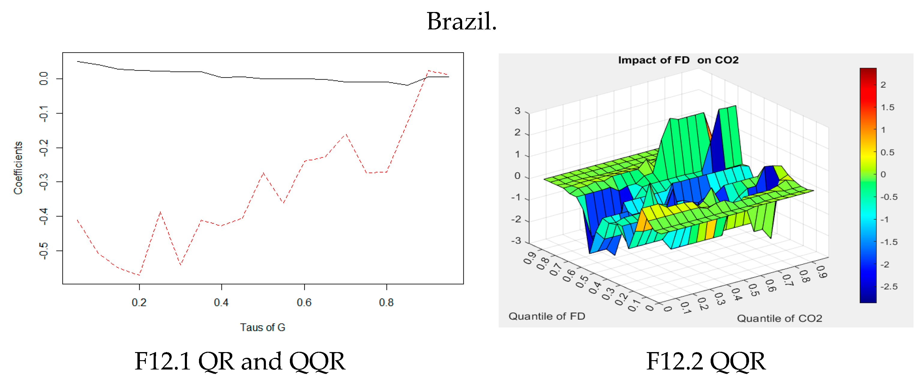
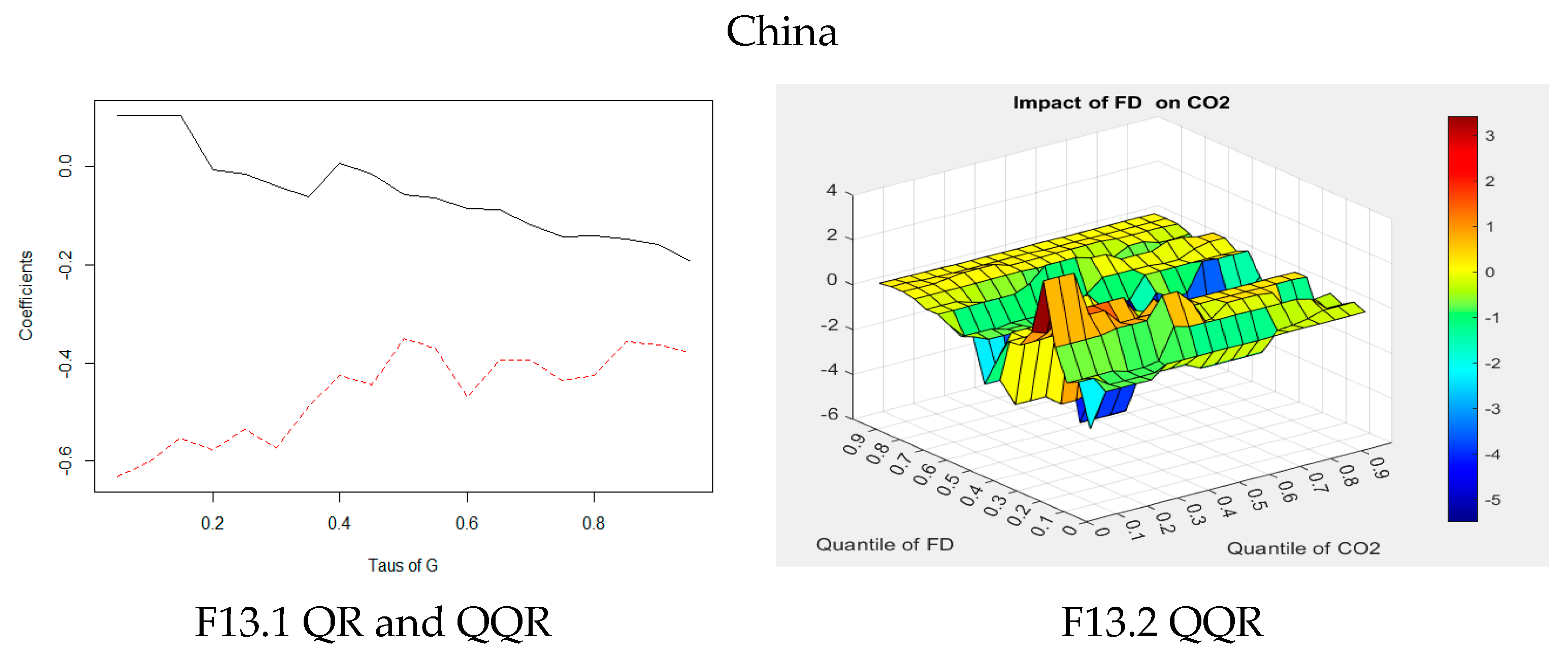
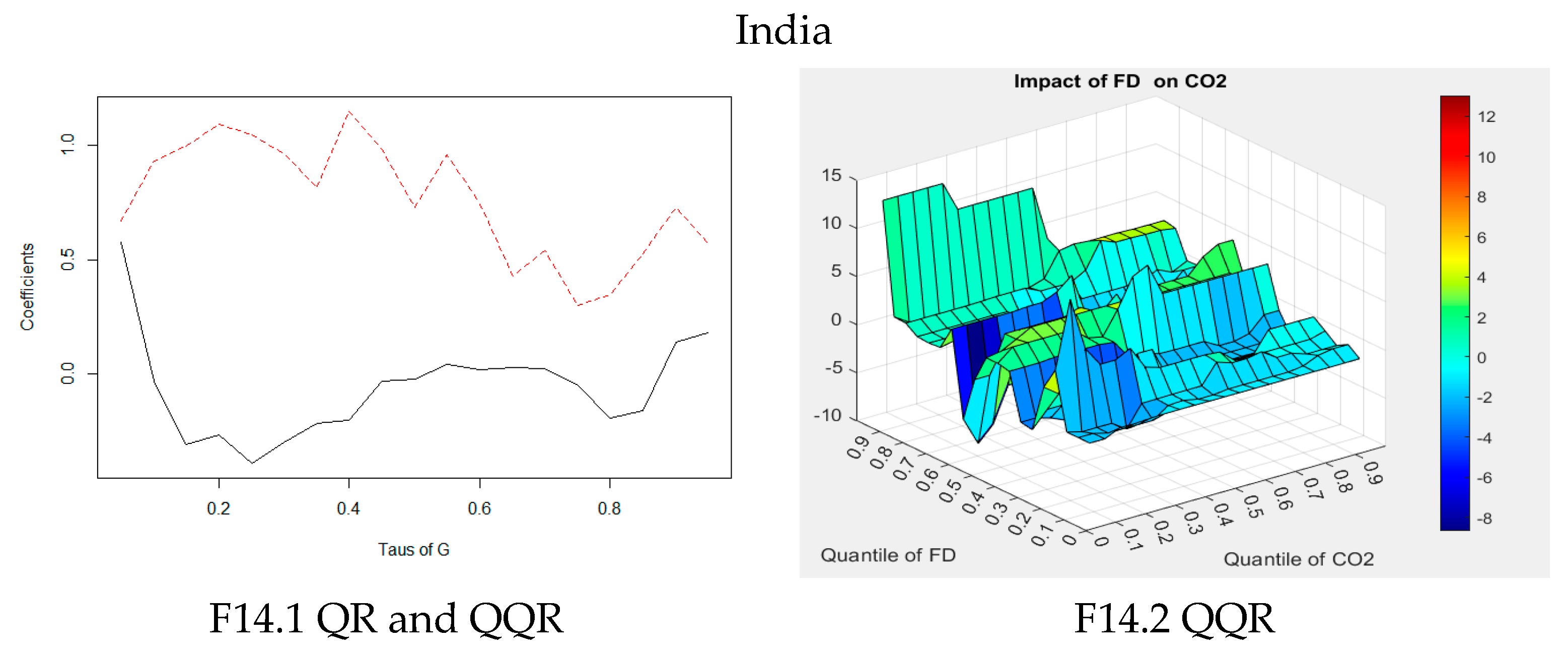
This paper investigated the relationship between carbon dioxide emissions, financial development, and economic growth in BRICS countries during the period 1976–2019. The Frontier Toda-Yamamoto QR with the smooth structure break and Quantile on Quantile methodologies, which were used to explore the EKC hypothesis in relation to the BRICS countries, represented the main innovative contributions of this paper.

Two important findings were made: first, there is a smooth structure break between CO₂ emissions and financial development in China and South Africa in the long-term under the EKC hypothesis. Second, in the short-term, from the QR at 0.6 quantile, Brazil’s CO₂ emissions have a positive impact on financial development. On a closer look at the quantile-on-quantile, Brazil’s CO₂ emissions in the 0.58–0.62 quantile were seen to have a strong positive impact on the financial development of the 0.68–0.72 quantile, while the financial development in the 0.63–0.67 quantile had a negative impact on CO₂ emissions in the 0.83–1 quantile, suggesting that Brazil’s environment is gradually improving in the short-term. India’s financial development in the 0.93–1 quantile had the strongest impact on CO₂ emissions in the low quantile (0–0.27), suggesting that India’s environmental emissions of CO₂ improved with financial development. It was found that the Chinese and South African governments’ policies were efficient in reducing CO₂ emissions and improving financial development because the policies of the two countries produced structural and transformational change between CO₂ emissions and financial development under economic growth in the long-term.

The conclusion is that financial development has a significant impact on CO₂ emissions, and this connection should be considered when formulating low-carbon policies. While ensuring the effective completion of low-carbon targets, the possible impact of CO₂ emission restrictions on the financial stability and stable economic growth of all countries should not be ignored.

References

1. Ledhem, M.A. Does Sukuk financing boost economic growth? Empirical evidence from Southeast Asia. PSU Res. Rev. 2020. ahead-of-print. [Google Scholar] [CrossRef]
2. Gani, I.M.; Bahari, Z. Islamic banking’s contribution to the Malaysian real economy. ISRA Int. J. Islamic Financ. 2021, 13, 6–25. [Google Scholar] [CrossRef]
3. Mollaahmetoğlu, E.; Akçalı, B.Y. The Missing-Link between Financial Development and Economic Growth: Financial Innovation. Procedia Comput. Sci. 2019, 158, 696–704. [Google Scholar] [CrossRef]
4. Olaniyi, C.O.; Adedokun, A. Finance-institution-growth trilogy: Time-series insights from South Africa. Int. J. Emerg. Mark. 2020. ahead-of-print. [Google Scholar] [CrossRef]
5. Le, H.P. The energy-growth nexus revisited: The role of financial development, institutions, government expenditure and trade openness. Heliyon 2020, 6, e04369. [Google Scholar] [CrossRef] [PubMed]
6. Song, C.-Q.; Chang, C.-P.; Gong, Q. Economic growth, corruption, and financial development: Global evidence. Econ. Model. 2020, 94, 822–830. [Google Scholar] [CrossRef]
7. Atil, A.; Nawaz, K.; Lahiani, A.; Roubaud, D. Are natural resources a blessing or a curse for financial development in Pakistan? The importance of oil prices, economic growth and economic globalization. Resour. Policy 2020, 67, 101683. [Google Scholar] [CrossRef]
8. Kapaya, S.M. Financial development and economic growth in Tanzania: An ARDL and bound testing approach. Asian J. Econ. Bank 2020. ahead-of-print. [Google Scholar] [CrossRef]
9. Moyo, C.; Le Roux, P. Financial development and economic growth in SADC countries: A panel study. Afr. J. Econ. Manag. Stud. 2020, 12, 71–89. [Google Scholar] [CrossRef]
10. Aluko, O.A.; Obalade, A.A. Financial development and environmental quality in sub-Saharan Africa: Is there a technology effect? Sci. Total Environ. 2020, 747, 141515. [Google Scholar] [CrossRef]
11. Nosheen, M.; Abbasi, M.A.; Iqbal, J. Analyzing extended STIRPAT model of urbanization and CO2 emissions in Asian countries. Environ. Sci. Pollut. Res. 2020, 27, 45911–45924. [Google Scholar] [CrossRef]
12. Odhiambo, N.M. Financial development, income inequality and carbon emissions in sub-Saharan African countries: A panel data analysis. Energy Explor. Exploit. 2020, 38, 1914–1931. [Google Scholar] [CrossRef]
13. Raghutla, C.; Chittedi, K.R. Financial development, energy consumption, technology, urbanization, economic output and carbon emissions nexus in BRICS countries: An empirical analysis. Manag. Environ. Qual. 2021, 32, 290–307. [Google Scholar] [CrossRef]
14. Umar, M.; Ji, X.; Kirikkaleli, D.; Xu, Q. COP21 Roadmap: Do innovation, financial development, and transportation infrastructure matter for environmental sustainability in China? J. Environ. Manag. 2020, 271, 111026. [Google Scholar] [CrossRef] [PubMed]
15. Nasir, M.A.; Canh, N.P.; Lan Le, T.N. Environmental degradation & role of financialisation, economic development, industrialisation and trade liberalisation. J. Environ. Manag. 2021, 277, 111471. [Google Scholar]
16. Shahbaz, M.; Nasir, M.A.; Hille, E.; Mahalik, M.K. UK’s net-zero carbon emissions target: Investigating the potential role of economic growth, financial development, and R&D expenditures based on historical data (1870–2017). Technol. Soc. Chang. 2020, 161, 120255. [Google Scholar]
17. Bui, D.T. Transmission channels between financial development and CO2 emissions: A global perspective. Heliyon 2020, 6, e05509. [Google Scholar] [CrossRef] [PubMed]
18. Wang, R.; Mirza, N.; Vasbieva, D.G.; Abbas, Q.; Xiong, D. The nexus of carbon emissions, financial development, renewable energy consumption, and technological innovation: What should be the priorities in light of COP 21 Agreements? J. Environ. Manag. 2020, 271, 111027. [Google Scholar] [CrossRef]
19. Lv, Z.; Li, S.S. How financial development affects CO2 emissions: A spatial econometric analysis. J. Environ. Manag. 2021, 277, 111397. [Google Scholar] [CrossRef] [PubMed]
20. Halliru, A.M.; Loganathan, N.; Golam Hassan, A.A.G.; Mardani, A.; Kamyab, H. Re-examining the environmental kuznets curve hypothesis in the economic community of West African states: A panel quantile regression approach. J. Clean Prod. 2020, 276, 124247. [Google Scholar] [CrossRef]
21. Kuznets, S. Economic Growth and Income Inequality. Am. Econ. Rev. 1955, 45, 1–28. [Google Scholar]
22. Panayotou, T. Empirical Tests and Policy Analysis of Environmental Degradation at Different Stages of Economic Development; ILO Working Papers 992927783402676; International Labour Organization: Geneva, Switzerland, 1993. [Google Scholar]
23. Yang, Z.; Abbas, Q.; Hanif, I.; Alharthi, M.; Taghizadeh-Hesary, F.; Aziz, B.; Mohsin, M. Short- and Long-Run Influence of Energy Utilization and Economic Growth on Carbon Discharge in Emerging SREB Economies. Renew. Energ. 2020, 165, 43–51. [Google Scholar] [CrossRef]
24. Sheng, P.; Li, J.; Zhai, M.; Huang, S. Coupling of economic growth and reduction in carbon emissions at the efficiency level: Evidence from China. Energy 2020, 213, 118747. [Google Scholar] [CrossRef]
25. Ardakani, M.K.; Seyedaliakbar, S.M. Impact of energy consumption and economic growth on CO2 emission using multivariate regression. Energy Strategy Rev. 2019, 26, 100428. [Google Scholar] [CrossRef]
26. Destek, M.A.; Shahbaz, M.; Okumus, I.; Hammoudeh, S.; Sinha, A. The relationship between economic growth and carbon emissions in G-7 countries: Evidence from time-varying parameters with a long history. Environ. Sci. Pollut. Res. 2020, 27, 29100–29117. [Google Scholar] [CrossRef] [PubMed]
27. Adebayo, T.; Akinsola, G.; Odugbesan, J.; Olanrewaju, V. Determinants of Environmental Degradation in Thailand: Empirical Evidence from ARDL and Wavelet Coherence Approaches. Pollution 2021, 7, 181–196. [Google Scholar]
28. Rahman, M.M.; Saidi, K.; Mbarek, M.B. Economic growth in South Asia: The role of CO2 emissions, population density and trade openness. Heliyon 2020, 6, e03903. [Google Scholar] [CrossRef]
29. Shahbaz, M.; Sharma, R.; Sinha, A.; Jiao, Z. Analyzing nonlinear impact of economic growth drivers on CO2 emissions: Designing an SDG framework for India. Energy Policy 2021, 148, 111965. [Google Scholar] [CrossRef]
30. Nair, M.; Arvin, M.B.; Pradhan, R.P.; Bahmani, S. Is Higher Economic Growth Possible Through Better Institutional Quality and a Lower Carbon Footprint? Evidence from Developing Countries. Renew. Energ. 2021, 167, 132–145. [Google Scholar] [CrossRef]
31. Sajo, A.I.; Li, B. Financial Development, Export and Economic Growth in Nigeria. Econ. Lett. 2017, 7, 2239–2254. [Google Scholar] [CrossRef] [Green Version]
32. Ofori-Abebrese, J.; Pickson, R.B.; Ofori-Abebrese, G. Commodity prices, exchange rate and economic growth in West Africa: Case study of Cote dIvoire and Ghana. J. Dev. Agric. Econ. 2017, 9, 269–277. [Google Scholar]
33. Maposa, L.; Muma, F.M. The Impact of Financial Development on Economic Growth in Zimbabwe: Comparative Analysis of Stock Markets and Commercial Banks. OA Lib. J. 2017, 4, 1–27. [Google Scholar] [CrossRef]
34. Botev, J.; Égert, B.; Jawadi, F. The nonlinear relationship between economic growth and financial development: Evidence from developing, emerging and advanced economies. Int. Econ. 2019, 160, 3–13. [Google Scholar] [CrossRef]
35. Ono, S. Financial development and economic growth nexus in Russia. Russ. J. Econ. 2017, 3, 321–332. [Google Scholar] [CrossRef] [Green Version]
36. Maji, I.K.; Habibullah, M.S.; Saari, M.Y. Financial development and sectoral CO2 emissions in Malaysia. Environ. Sci. Pollut. Res. 2017, 24, 1–17. [Google Scholar] [CrossRef] [PubMed]
37. Bayar, Y.; Diaconu, L.; Maxim, A. Financial Development and CO2 Emissions in Post-Transition European Union Countries. Sustainability 2020, 12, 2640. [Google Scholar] [CrossRef] [Green Version]
38. Baloch, M.A.; Danish, F.M.; Zhang, J.; Xu, Z. Financial instability and CO2 emissions: The case of Saudi Arabia. Environ. Sci. Pollut. Res. 2018, 25, 26030–26045. [Google Scholar] [CrossRef] [PubMed]
39. Khan, A.Q.; Saleem, N.; Fatima, S.T. Financial development, income inequality, and CO2 emissions in Asian countries using STIRPAT model. Environ. Sci. Pollut. Res. 2018, 25, 6308–6319. [Google Scholar] [CrossRef] [PubMed]
40. Ahmad, M.; Khan, Z.; Rahman, Z.U.; Khan, S. Does financial development asymmetrically affect CO2 emissions in China? An application of the nonlinear autoregressive distributed lag (NARDL) model. Carbon Manag. 2019, 9, 631–644. [Google Scholar] [CrossRef]
41. Yildirim, H.H. Economic Growth and CO2 Emissions for OECD Countries. Int. J. Manag. Sci. Bus. Adm. 2017, 3, 30–37. [Google Scholar]
42. Ozcan, B.; Tzeremes, P.G.; Tzeremes, N.G. Energy consumption, economic growth and environmental degradation in OECD countries. Econ. Model 2020, 84, 203–213. [Google Scholar] [CrossRef]
43. Kahouli, B. The causality link between energy electricity consumption, CO2 emissions, R&D stocks and economic growth in Mediterranean countries (MCs). Energy 2018, 145, 388–399. [Google Scholar]
44. Liu, J.L.; Ma, C.Q.; Ren, Y.S.; Zhao, X.W. Do real output and renewable energy consumption affect CO2 emissions? Evidence for selected BRICS countries. Energies 2020, 13, 960. [Google Scholar] [CrossRef] [Green Version]
45. Baydoun, H.; Aga, M. The Effect of Energy Consumption and Economic Growth on Environmental Sustainability in the GCC Countries: Does Financial Development Matter? Energies 2021, 14, 5897. [Google Scholar] [CrossRef]
46. Szymczyk, K.; Şahin, D.; Bağcı, H.; Kaygın, C.Y. The Effect of Energy Usage, Economic Growth, and Financial Development on CO2 Emission Management: An Analysis of OECD Countries with a High Environmental Performance Index. Energies 2021, 14, 4671. [Google Scholar] [CrossRef]
47. Zhang, Y. Structural decomposition analysis of sources of decarbonizing economic development in China; 1992–2006. Ecol. Econ. 2009, 68, 2399–2405. [Google Scholar] [CrossRef]
48. Boutabba, M.A. The impact of financial development, income, energy and trade on carbon emissions: Evidence from the Indian economy. Econ. Model. 2014, 40, 33–41. [Google Scholar] [CrossRef] [Green Version]
49. Shahbaz, M.; Mallick, H.; Mahalik, M.K.; Loganathan, N. Does globalization impede environmental quality in India? Ecol. Indic. 2015, 52, 379–393. [Google Scholar]
50. Tamazian, A.; Chousa, J.P.; Vadlamannati, K.C. Does higher economic and financial development lead to environmental degradation: Evidence from BRIC countries. Energy Policy 2009, 37, 246–253. [Google Scholar] [CrossRef]
51. Jalil, A.; Feridun, M. The impact of growth, energy and financial development on the environment in China: A cointegration analysis. Energy Econ. 2011, 33, 284–291. [Google Scholar] [CrossRef]
52. Yuxiang, K.; Chen, Z. Resource abundance and financial development: Evidence from China. Resour. Policy 2011, 36, 72–79. [Google Scholar] [CrossRef]
53. Zhang, J.; Wang, L.; Wang, S. Financial development and economic growth: Recent evidence from China. J. Comp. Econ. 2012, 40, 393–412. [Google Scholar] [CrossRef]
54. Ahmed, K.; Jahanzeb, A. Does financial development spur environmental and energy-related innovation in Brazil? Int. J. Financ. Econ. 2021, 26, 1706–1723. [Google Scholar]
55. Cai, Y.; Sam, C.Y.; Chang, T. Nexus between clean energy consumption, economic growth and CO2 emissions. J. Clean. Prod. 2018, 182, 1001–1011. [Google Scholar] [CrossRef]
56. Lin, F.L.; Inglesi-Lotz, R.; Chang, T. Revisit coal consumption, CO2 emissions and economic growth nexu in China and India using a newly developed bootstrap ARDL bound test. Energy Explor. Exploit. 2018, 36, 450–463. [Google Scholar] [CrossRef] [Green Version]
57. Goh, S.K.; Tang, T.C.; Sam, C.Y. Are Major US Trading Partners’ Exports and Imports Cointegrated? Evidence from Bootstrap ARDL. Margin. J. Appl. Econ. Res. 2020, 14, 7–27. [Google Scholar] [CrossRef]
58. Gallant, A.R. On the bias in flexible functional forms and an essentially unbiased form: The fourier flexible form. J. Econom. 1981, 15, 211–245. [Google Scholar] [CrossRef]
59. Gallant, A.R.; Souza, G. On the asymptotic normality of Fourier flexible form estimates. J. Econom. 1991, 50, 329–353. [Google Scholar] [CrossRef] [Green Version]
60. Akaike, H. Maximum likelihood identification of Gaussian autoregressive moving average models. Biometrika 1973, 60, 255–265. [Google Scholar] [CrossRef]
61. Hatemi-J, A.; Uddin, G.S. Is the causal nexus of energy utilization and economic growth asymmetric in the US? Econ. Syst. 2012, 36, 461–469. [Google Scholar] [CrossRef]
62. Bayer, C.; Hanck, C. Combining non-cointegration tests. J. Time Ser. Anal. 2013, 34, 83–95. [Google Scholar] [CrossRef]
63. Engle, R.F.; Granger, C.W.J. Co-Integration and Error Correction: Representation, Estimation, and Testing. Econometrica 1987, 55, 251–276. [Google Scholar] [CrossRef]
64. Johansen, S. Estimation and hypothesis testing of cointegration vectors in Gaussian vector autoregressive models. Econom. J. Econom. Soci. 1991, 59, 1551–1580. [Google Scholar] [CrossRef]
65. Boswijk, H.P. Testing for an unstable root in conditional and structural error correction models. J. Econom. 1994, 63, 37–60. [Google Scholar] [CrossRef]
66. Banerjee, A.; Dolado, J.; Mestre, R. Error-correction mechanism test for cointegration in a single-equation framework. J. Time Ser. Anal. 1998, 19, 267–283. [Google Scholar] [CrossRef] [Green Version]
67. Fisher, I. Booms and Depressions: Some First Principles (Adelphi, New York) 1932. Energy International Agency (EIA), 2014. Available online: https://www.eia.gov/beta/international/country.cfm?iso=IRN (accessed on 11 March 2021).
68. Sim, N.; Zhou, H. Oil prices, US stock return, and the dependence between their quantiles. J. Bank Financ. 2015, 55, 1–8. [Google Scholar] [CrossRef]
69. Granger, C.W.; Yoon, G. Hidden Cointegration. U of California, Economics Working Paper No. 2002-02. 2002. Available online: https://papers.ssrn.com/sol3/papers.cfm?abstract_id=313831 (accessed on 20 August 2021).
70. Hatemi-J, A. Asymmetric causality tests with an application. Empir. Econ. 2012, 43, 447–456. [Google Scholar] [CrossRef]
71. Bahmani-Oskooee, M.; Chang, T.; Niroomand, F.; Ranjbar, O. Fourier nonlinear quantile unit root test and PPP in Africa. Bull. Econ. Res. 2020, 72, 451–481. [Google Scholar] [CrossRef]
Figure 1. The global GDP share of the BRICS countries.
Energies 14 07341 g001
Figure 2. Per capita GDP of BRICS countries (unit: person/USD).
Energies 14 07341 g002
Figure 3. Annual GDP growth rate of the BRIC countries.
Energies 14 07341 g003
Figure 4. Broad money M2 (% of GDP).
Energies 14 07341 g004
Figure 5. Total assets of the BRICS banking industry Unit: US$ million (up to February 2021).
Energies 14 07341 g005
Figure 6. The ratio of bank non-performing loans to total loans (%).
Energies 14 07341 g006
Figure 7. The stock trading turnover rate (%).
Energies 14 07341 g007
Figure 8. World shares of total CO2 emissions (million tons).
Energies 14 07341 g008
Figure 9. The primary energy consumption of BRICS countries (hundreds of billions of joules).
Energies 14 07341 g009
Figure 10. Per capita CO2 emissions (tons per capita).
Energies 14 07341 g010
Figure 11. Curves of economic growth, FD, and CO2 emissions in BRICS countries.
Energies 14 07341 g011
Figure 12. Analysis of QR and QQR in India Brazil.
Energies 14 07341 g012
Figure 13. Analysis of QR and QQR in China.
Energies 14 07341 g013
Figure 14. Analysis of QR and QQR in India.
Energies 14 07341 g014
Figure 15. Analysis of QR and QQR in South Africa.
Energies 14 07341 g015