Improving Forecast Reliability for Geographically Distributed Photovoltaic Generations

Abstract

Photovoltaic (PV) generation is potentially uncertain. Probabilistic PV generation forecasting methods have been proposed with prediction intervals (PIs) to evaluate the uncertainty quantitively. However, few studies have applied PIs to geographically distributed PVs in a specific area. In this study, a two-step probabilistic forecast scheme is proposed for geographically distributed PV generation forecasting. Each step of the proposed scheme adopts ensemble forecasting based on three different machine-learning methods. When individual PV generation is forecasted, the proposed scheme utilizes surrounding PVs’ past data to train the ensemble forecasting model. In this case study, the proposed scheme was compared with conventional non-multistep forecasting. The proposed scheme improved the reliability of the PIs and deterministic PV forecasting results through 30 days of continuous operation with real data in Japan.

1. Introduction

Photovoltaic (PV) generation in a distribution network plays a key role in promoting clean energy production. One of the well-recognized problems of the PV generation is the increased power flow at the substation and in the distribution line under the substation [1]. The peak time and the amount of power flow depend on the demand and PV generation in the network. The peak is mitigated by energy storage systems (ESSs) operations, such as fixed batteries reported in [2,3]. The peak time and energy generated from the PVs must be forecasted to operate the ESS with the best efficiency. In [3], the proposed peak-shaving algorithm is performed based on prediction intervals (PIs) and indicates the probability of peak demand at the substation. The PIs are evaluated using two fundamental but contradictory ideas: the coverage rate and the width of the intervals [4]. If the PIs cover all observations, the coverage rate is the best at 100%. By contrast, the PI widths are preferred to be narrower. As the PIs have a high coverage rate of observations and become narrower, the performance of the peak mitigation improves [3].

PVs are distributed within a specific area connected to the same distribution network. Thus, a spatiotemporal model is required to extract and use spatial and temporal data from multiple PVs to improve PI reliability [5,6,7]. The authors of [5] proposed a deep learning framework that can generate PV forecasts for multiple regions and horizons with 56 locations in the US, while [6] proposed a model to forecast six hours based on 136 PV installations in France. Irradiance forecasting for 11 PVs distributed in a specific region is performed as accumulated generations [8]. The cloud motion vector-based method [9,10] is an established approach for covering distributed PVs in a specific area. Numerical weather predictions are used for forecasting hours to days ahead [11]. Satellite images, ground measurements, and sky imaging were combined to improve deterministic and probabilistic forecast reliability [12]. In [13], optical flow deals with nonuniform cloud motion and is originally a technique for image processing [14]. The optical flow is a distribution of the apparent velocities of the movement of brightness patterns in an image. An optical flow that tracks the amount of distributed PV generation was developed in our laboratory [15]. Consequently, the mean absolute percentage error is 4.23% in the case of forecasting 30 min [15]. However, the error increases when the prediction time is extended.

Another promising approach for forecasting PV generation is the historical data-driven approach. Data-driven approaches require a large amount of measured past-generation data for deep learning [16]. However, once the correct dataset with a small number of missing records is arranged, the forecasting ability is excellent, especially in day-ahead forecasting [17]. Developing PIs with data-driven approaches for various objectives, not including PV forecasting, is proposed based on Delta [18,19], Bayesian [20], mean-variance estimation [21], and bootstrap techniques [22], which are comprehensively compared in [23]. Quantile regression was adopted in [7]. The bootstrap technique was proposed in [17] to quantify the uncertainty with PIs for PV forecasting. In addition, the performance of the bootstrap technique has been proven for wind farm power generation forecasts [24].

As aforementioned, sky or cloud image-based methods and data-driven approaches have been developed; however, according to the intensive reviews of PV forecasting reported in [11], studies on regional models for multiple PVs are limited. Most studies have focused on forecasting at single locations, while little work has been done on regional models. The few PV forecasting studies for distributed PVs did not focus on the individual PV generation forecast but accumulated total PV generation in the region. In addition, the existing forecast models are too specific to circumscribe to a particular region [25]. The model and the methodology to individually forecast the distributed PV generation is required, not limited to the specific circumstances to a particular region.

This study developed and verified a two-step probabilistic forecast scheme for geographically distributed PV generation forecasting. We introduce the idea of optical flow to data-driven methods, such as machine-learning-based methods, to improve existing probabilistic PV generation forecasting methods. Existing machine learning utilizes past data, including generations, temperature, humidity, and precipitation, and the most important predictor is radiation. The forecasting model was mainly developed for each PV system. Conversely, the original idea of PV generation forecasting, with the optical flow developed in our laboratory, is that the generation of geographically distributed PVs moves as the sun and clouds move [15].

Herein, we propose a PV forecasting method for geographically distributed PVs in a specific area. The PVs are geographically close. Therefore, the past-generation data of one PV can be a meaningful predictor of another PV generation forecasting, which is proven in Section 3 as a case study. Ensemble forecasting comprising three machine-learning methods is proposed in this study as an example of probabilistic forecasting. The proposed ultimate forecasting scheme comprises a single PV forecast model and multiple PV forecast models. The ensemble forecast was adopted for both single and multiple PV forecast models. The proposed ensemble method is enhanced by utilizing the past-generation data of multiple PVs. The simulation shows that the reliability of the forecasting is improved by both deterministic and probabilistic forecasting. The contributions of this study are as follows:

(1)

We propose a method to develop boundaries for PIs based on past forecast errors. The case study shows that the boundaries are stable and functional for multiple PVs based on actual PV generation data.

(2)

A multi-step PV forecasting scheme for geographically distributed PVs in a specific area is proposed. The case study shows that the proposed scheme improves the forecasting reliability with real PV generation data.

(3)

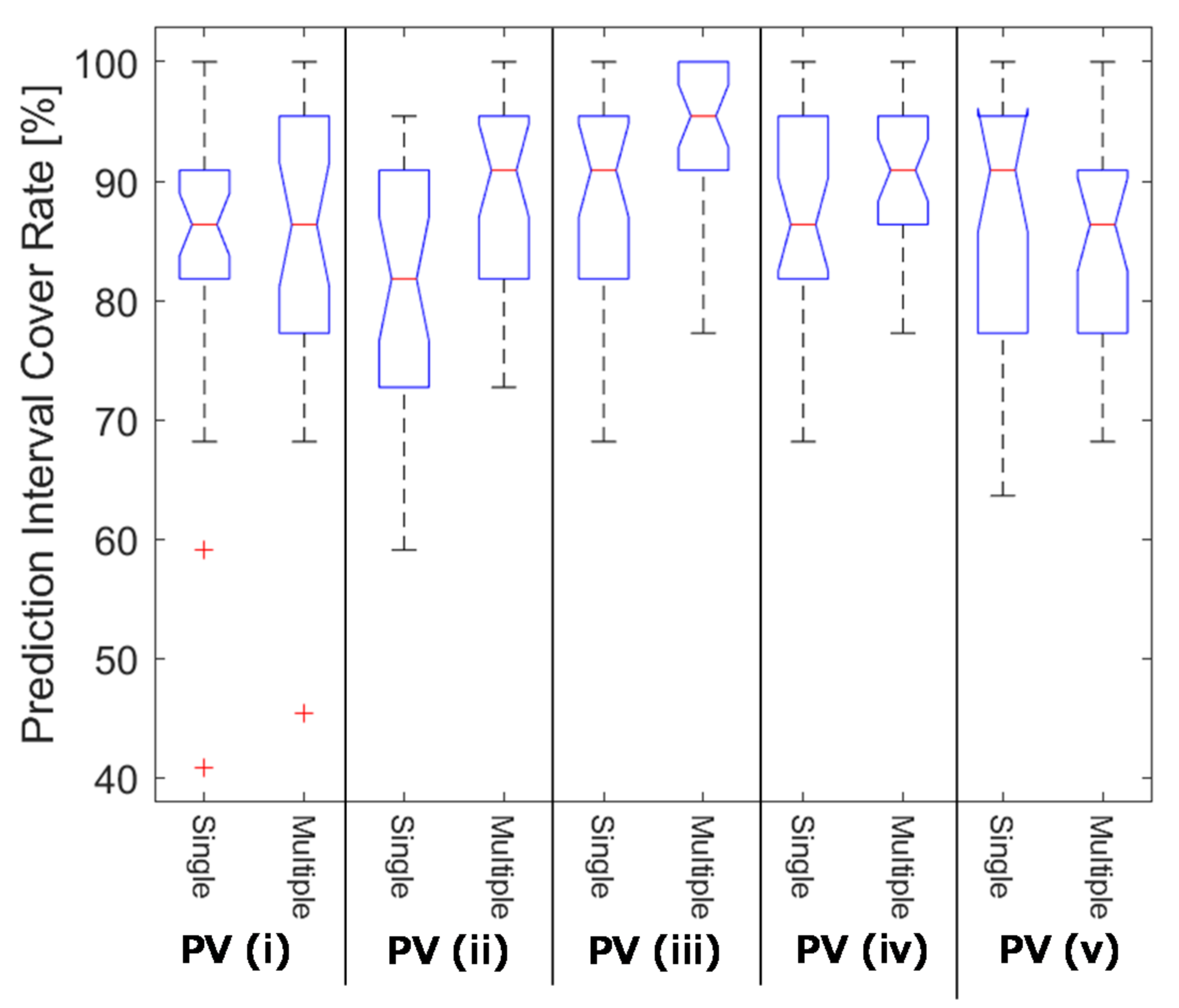
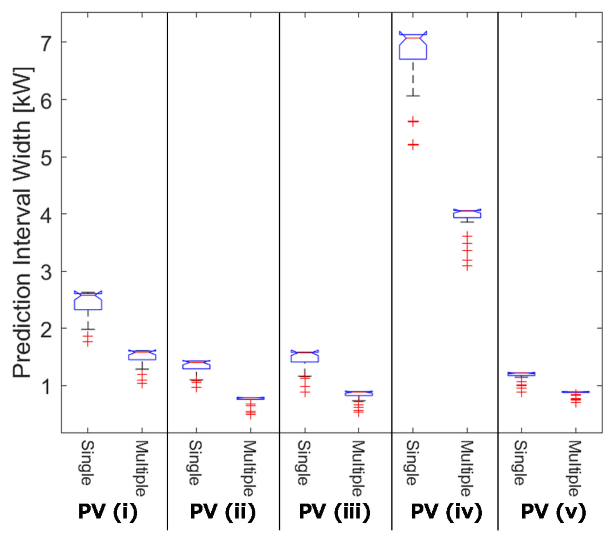
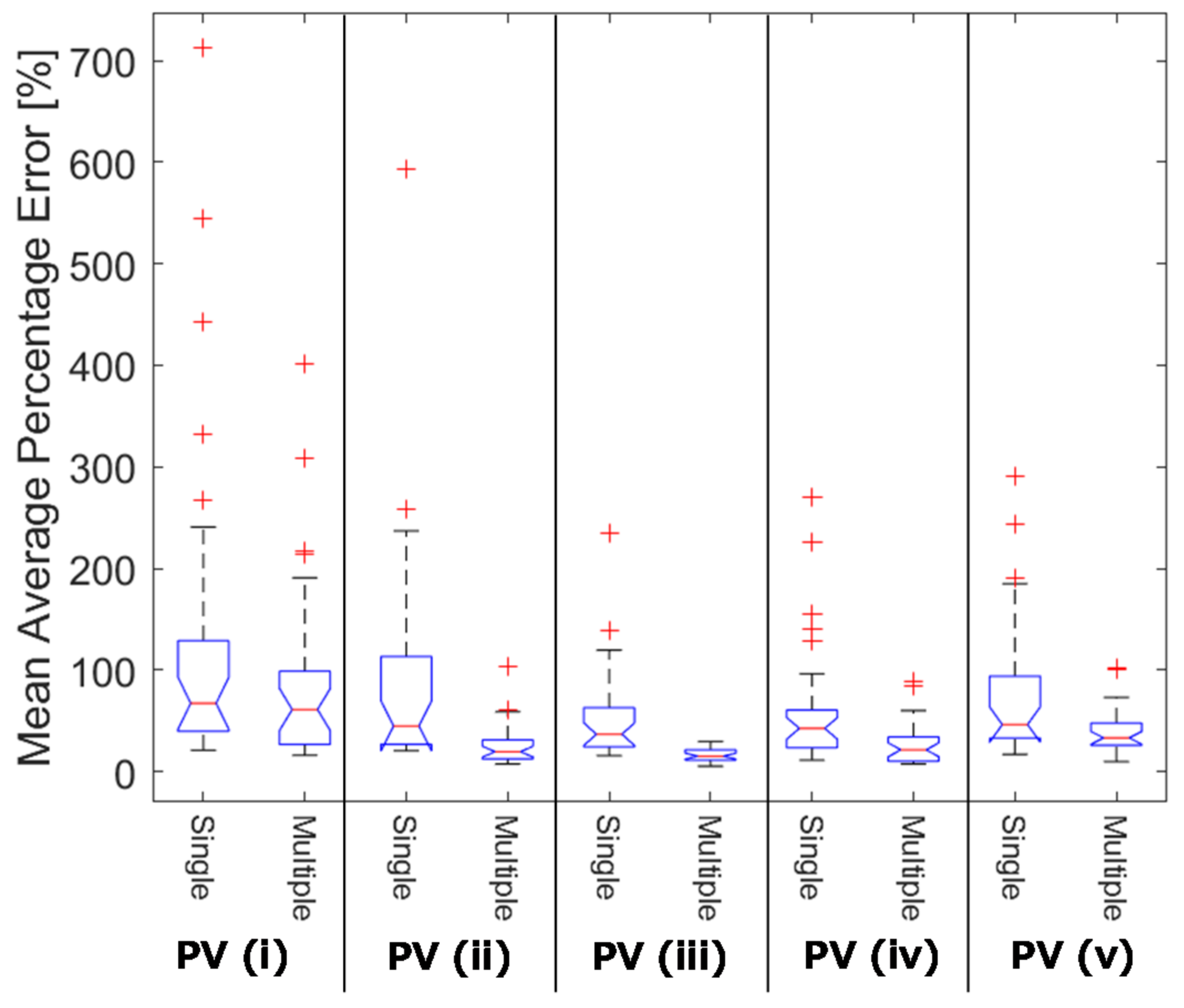
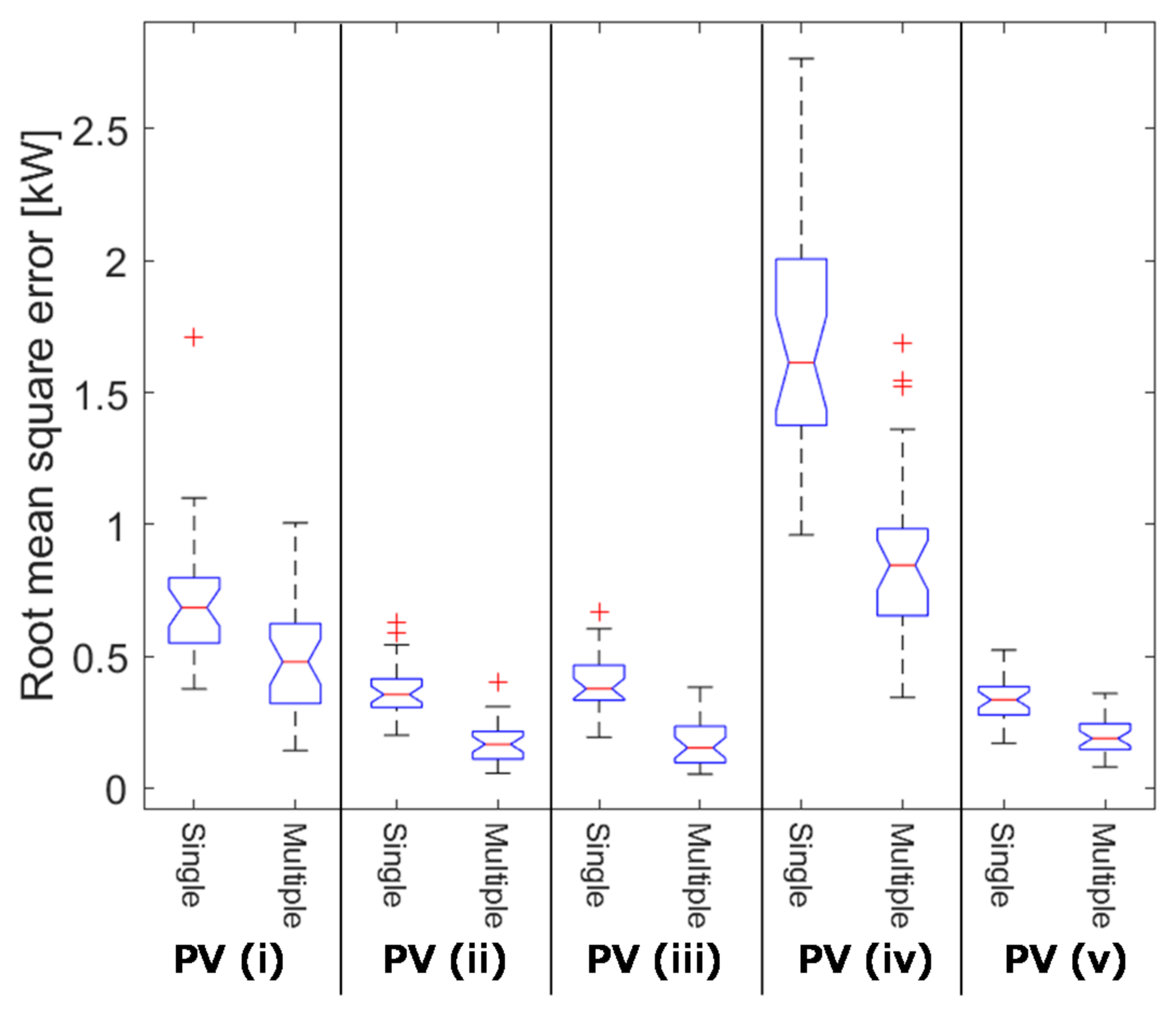
The performance of the proposed multi-step PV forecasting scheme was evaluated with a long-term simulation case as continuous 30 days. The statistical analysis indicates that the proposed scheme improves the root mean square error (RMSE) and mean average percentage error (MAPE) for deterministic forecasting. In addition, the PI cover rate and the width of the PI for probabilistic forecasting are improved compared to conventional single PV forecast methods.

The rest of the paper is organized as follows: Section 2 introduces the methodology of the ensemble forecasting model and the way to generate the PIs. Section 3 introduces the case study to prove that the proposed forecasting algorithms can improve the reliability of probabilistic forecasting in terms of the PI cover rate and PI width. Finally, Section 4 concludes the study.

2. Forecast Methodology

The proposed forecast model comprises two steps: a single-forecast model and a multiple forecast model, as shown in Figure 1. The single-forecast model is composed for each PV, indicated as $P{V}_1$, $P{V}_2$, … $P{V}_i$ in Figure 1. Past-generation data and weather data are inputs for the ensemble forecast model, as explained in Section 2.1. The forecasted PV generation by the single-forecast model for each PV was utilized as inputs to the multiple forecast model. In Figure 1, $P{V}_{i+1}$ is forecasted based on the forecasted generation from $P{V}_1$ to $P{V}_i$, which were chosen based on the Euclidean distance calculated by the latitude and longitude of each PV location. In the case study, the five nearest PVs were chosen to compose the multiple forecast models. The multiple forecast model is performed based on the past data of the target PV, weather data, and the results of other PV forecasts by the single-forecast models.

2.1. Ensemble Forecasting with Prediction Intervals

Both the single and multiple PV forecast models were designed for ensemble forecasting. Three data-driven regressions, naive Bayes classifier, neural network (NN), and long short-term memory (LSTM), are utilized for ensemble forecasting. In this study, we handle multiple PVs that are geographically distributed in a specific area. The ensemble model is arranged for each PV in the proposed method. If we need to forecast five PVs at once, we need to build five individual models for each PV based on different training data. The configuration of the ensemble model is shown in Figure 2. Each data-driven regression model was individually trained to configure the best parameters based on past data. All individual models were added with different weights and one ensemble model. The weight optimizer in Figure 2 calculates the optimal weight for addition based on the past performance of each model. The naive Bayes classifier-based prediction was reported in [26]. The NN model was designed using the function-fitting neural network available in MATLAB [27]. LSTM was also implemented using the function in MATLAB [28].

The PV forecast process is assumed to be performed once a day using continuously updated observed data. The forecast result is provided as day-ahead forecasting; hence, the forecasted PV generation can be utilized to determine the operations of the ESS charge and discharge [3]. The process of ensemble forecasting, and the development of the prediction intervals, are shown in Figure 3. The PV forecasting process comprises two parts: the training process with past data and the forecasting process with test data. The implementation codes of MATLAB for the model in Figure 3 are available on GitHub [29]. The steps from (i) to (vi) in Figure 3 are explained as follows.

(i)

Check if forecast models need to be updated

In step (i), the ensemble forecast model is inspected to check whether the trained parameters are the latest. If the trained model with the determined parameters does not include the latest observed data, the model is re-trained to update the parameters of every forecasting method. In the training process, the parameters for the ensemble forecasting methods are determined using past data. Once the training process is completed, the parameters for the forecasting methods remain fixed until a new training process is performed. Therefore, the model parameters must be updated periodically to catch up with the latest observed data. In the case study, the model was updated every 30 days.

(ii)

Train each forecast model with training data

In step (ii), the forecasting models naive Bayes classifier, NN, and LSTM are individually trained. The data configuration is shown in Figure 4. Two groups are arranged for model building and forecasting: long-term past data (training and validation data) and forecast data. Long-term data contain predictors (timestamps, temperature, and weather conditions) and target (PV generation); forecast data contain only predictors. In the forecast data, weather information is obtained from weather forecasts available to the public via the web. Training data were utilized as a training dataset to construct the naive Bayes classifier, NN, and LSTM models. Long-term past data preferably contain at least one year of collection to capture seasonal features. Validation data in the long-term past data were selected in sets of arbitrary length from long-term past data. The validation data were utilized to determine the optimal weight for the ensemble forecast model, as shown in Figure 2. In addition, the validation data are utilized to compose the error distribution, leading to PIs. Based on the validation data, the error distribution can reveal bias errors caused by recent facility changes, such as installing new PV farms [30]. This bias error can also be reflected in model training with long-term past data, including validation data. However, the significance of the error takes more than several weeks to show up because the biased new data records are significantly smaller than the existing long-term past data.

The NN model comprises four hidden layers with 20, 20, 20, and 15 units, respectively. Scaled conjugate gradient [31] is utilized as a training function. The forecast result in every time step is obtained by taking the average of three times to mitigate the affection of initial value randomness.

The LSTM model comprises three hidden layers that have 100, 50, and 25 units, respectively. The maximum number of epochs is 250, the gradient threshold is 1.2, the initial learning rate used for training is 0.01, the number of epochs for dropping the learning rate is 125, and the factor for dropping the learning rate is 0.2.

The k-means method is utilized to classify the training data, and the classified training data is an input for the naive Bayes classifier. Naive Bayes classifier provides the PV forecasting. The k-means and naive Bayes classifier combined to forecast the PV generation as follows:

Step 1.

k-means classifies the observed PV generation records with 50 clusters. In this case, the k = 50 is experimentally chosen. Then, the predictors such as temperature and weather conditions corresponding with each timestamp are classified in each cluster.

Step 2.

Train naive Bayes classifier model by the classified observed and kernel distribution function for predictors.

Step 3.

The trained naive Bayes classifier classifies the unknown predictors as test data with each cluster.

Step 4.

The centroid of each cluster, which is determined in Step1, is the forecasted PV generation value.

(iii)

Find the best weight for each forecast model

The optimal coefficients for an ensemble model composed of these two trained models were determined. For the naive Bayes classifier model, an optimal k is determined, which indicates how many groups need to be generated. The NN model learns the weights of each neuron. An ensemble prediction model was built by combining these two prediction models with weights, as shown in Equation (1):

$${\widehat{y}}_t^i={\displaystyle \sum }_{i=1}^N{c}_t {\widehat{F}}_t^i, i\in N,t\in T$$

(1)

Here, ${\widehat{y}}_t^i$ is the ultimate deterministic forecasted value of PV generation for time instance t on the i-th day. T is the time instances in a day, which is 48 times in the case study. N is defined as the number of days for error validation indicated by N in Figure 4. ${\widehat{F}}_t^i$ is the deterministically forecasted PV generation using the individual forecast methods at time t. In this case, three methods (N = 3) were adopted: naive Bayes classifier, NN, and LSTM. The coefficients $c_t$ are the weights of each forecasting method. $c_t$ is common for all days N. The weights are time-consistent, as determined by the particle swarm optimization (PSO) algorithm that minimizes the error between the observed and predicted loads, as shown in Equation (2):

$$\mathit{a}\mathit{r}\mathit{g} \underset{c_t}{\mathbf{min}} \Vert {\mathbb{Y}}_i-{\widehat{\mathbb{Y}}}_i{\Vert }_2$$

(2)

Here,

$$\begin{array}{c}{\mathbb{Y}}_i:=\left\{y_1^i, y_2^i, \dots y_{\mathrm{t}}^i\dots y_T^i\right\}\\ {\widehat{\mathbb{Y}}}_i:=\left\{{\widehat{y}}_1^i,{\widehat{y}}_2^i, \dots {\widehat{y}}_{\mathrm{t}}^i\dots {\widehat{y}}_T^i\right\}\end{array}$$

(3)

${\mathbb{Y}}_i$ is the set of observed data $y_t^i$ corresponding to the predicted PV generation ${\widehat{y}}_t^i$ at time $t$ on the i-th day, and ${\widehat{\mathbb{Y}}}_i$ is the set of predicted PV generation ${\widehat{y}}_t^i$. For instance, as shown in Figure 5, if the observed data comprise 30 min-intervals, $t$ comprises 48 instances a day. The deterministic prediction by the ensemble model is performed for past data for a specific time duration, such as the period of one year (i = 1, 2, 3, …, 365).

(iv)

Derive error distribution from the ensemble model

Once the optimal coefficients are obtained, future PV generation is forecasted using the trained ensemble model. The boundaries of the PIs were subsequently calculated. The absolute error set ${\mathbb{E}}_t$ for a specific time $t$ is derived by comparing the predicted and observed data throughout the short-term past data. A series of errors are indicated in Figure 5, and the error set is expressed as follows:

$$e_t^i=y_t^i-{\widehat{y}}_t^i$$

(4)

$${\mathbb{E}}_t:=\left\{e_t^1, e_t^2, e_t^3\dots e_t^i\dots e_t^N\right\}, i\in N, t\in T$$

(5)

Here, $e_t^i$ is the forecasting error for the i-th day at time $t$. N indicates the number of days included in the validation dataset. Each time $t$ has an error record for several days. The set ${\mathbb{E}}_t$ forms the histogram for each time $t$ and is referred to as the error distribution in this document.

(v)

Forecast deterministic PV generation by the ensemble model

After the error distribution is formulated in the model training process, deterministic PV generation is forecasted for the next 24 h. The deterministic forecast and error distribution were added into a set ${\mathbb{D}}_t$. The set ${\mathbb{D}}_t$ for time t is defined as follows:

$${\mathbb{D}}_t:=\left\{{\widehat{y}}_t+e_t^1, {\widehat{y}}_t+e_t^2, {\widehat{y}}_t+e_t^3\dots {\widehat{y}}_t+e_t^N\right\}$$

(6)

(vi)

Make prediction interval from error distribution and deterministic forecasting

The PIs comprise upper and lower boundaries. In this study, these boundaries are obtained by taking confidence intervals from set ${\mathbb{D}}_t$ in (6). The set ${\mathbb{D}}_t$ is not guaranteed to be distributed as a normal distribution; thus, making PIs should be investigated further in future work. In the following case study, the confidence interval level is 95% as an example, which can change as the application requires.

2.2. Multiple Forecast Model

The multiple forecast models have the same ensemble model as the single-forecast models. The operation flow of the multiple forecast model is also similar to that of the single PV forecast model, as shown in Figure 3. The difference between the multiple and single-forecast models is the input data into the ensemble models, as shown in Figure 1. First, the target PV was chosen as the output of the multiple PV forecast model. Second, the PVs forecasted by the single PV forecast models were selected based on the geographical distance from the target PV. In the case study, four PVs were selected for the single-forecast model as an example. The criteria that choose PVs for the single-forecast model are still open to discussion and can consider the ground form, the direction of the PV panels, obstacle conditions (sometimes the building makes shade for PV panels at a specific time), and others. The correlation coefficient between the generation data from the target PV and PVs for the single PV forecast model is a promising candidate for choosing PVs for a single PV forecast model.

3. Case Study

3.1. Given Data Set and Premises

The data were collected around the Kanto region in Japan. The observed points were distributed as shown in Figure 6. PV generation is forecasted for five PVs named PV (i), (ii), (iii), (iv), and (v) to validate that the proposed multiple PV forecast model improves the reliability of the forecasting for each PV generation. The rates of power of PVs are: (i) 4.80 kW, (ii) 2.88 kW, (iii) 3.42 kW, (iv) 20.09 kW, and (v) 3.00 kW, respectively. PV generation was observed every 30 min from 6:30 a.m. to 5:00 p.m. daily. The observed generation data are recorded with year, month, day, hour, minutes, temperature, precipitation, and weather (sunny, cloud, or rain). The location of each PV is also given by latitude and longitude. These five PVs are chosen to be close to each other in terms of distance. The distances between each PV are shown in Figure 6. The area PVs are almost flat; therefore, the altitude is assumed to be the same in the case study.

The observed data for the case study are from 15 August 2013 to 31 July 2014. The PV generation for each PV is forecasted using a single PV forecast model and a multiple PV forecast model. The one-day-ahead forecasting is continuously performed for 30 days from 2 July 2014 to 31 July 2014. Due to the limited data aquation from the system, the observed data from 10:30 pm to 6:00 am are not available; therefore, the data from 5:30 p.m. to 10:00 p.m. are not utilized for model training and forecasting. There are no reasons to restrict the data in a day from the viewpoint of the proposed algorithm or model. The data for all the time in a day is the ideal data set for more accurate forecast models. Some missing records from 10:30 p.m. to 6:00 a.m. were interpolated by linear interpolation. The PV forecast error increases with interpolated training data than the PV forecast with no missing records in the training data. In [32], four imputation methods to fill the missing records are evaluated for the PV generation forecasting. According to [1], the PV generation forecasting with 10% interpolated records by linear interpolation leads to the 0.17% higher mean relative error than the forecasting with no missing records. On the other hand, the ratio of the missing records in all data for each PV unit in this study is shown in

Table 1. The ratio of the missing records for each PV in all past data.

PV ID	The Number of Total Records	The Number of Missing Record	Missing Rate [%]
(i)	7722	494	6.4
(ii)	7722	754	9.8
(iii)	7722	410	5.3
(iv)	7722	188	2.4
(v)	7722	864	11.2

. Table 1 shows that every PV data contains around 10% or less than 10% missing records. These missing records are filled by linear interpolation. Therefore, the missing records affect the forecast accuracy around 0.17%, as [1] shows, which is not significant to the forecast result in the study.

3.2. Simulation Results

The simulation result is evaluated based on four criteria: the cover rate of the prediction interval, the width of the prediction interval, MAPE, and RMSE. The forecasted result is calculated daily with a 30-min interval because the ESSs in distribution networks are assumed to operate following the predetermined schedule daily.

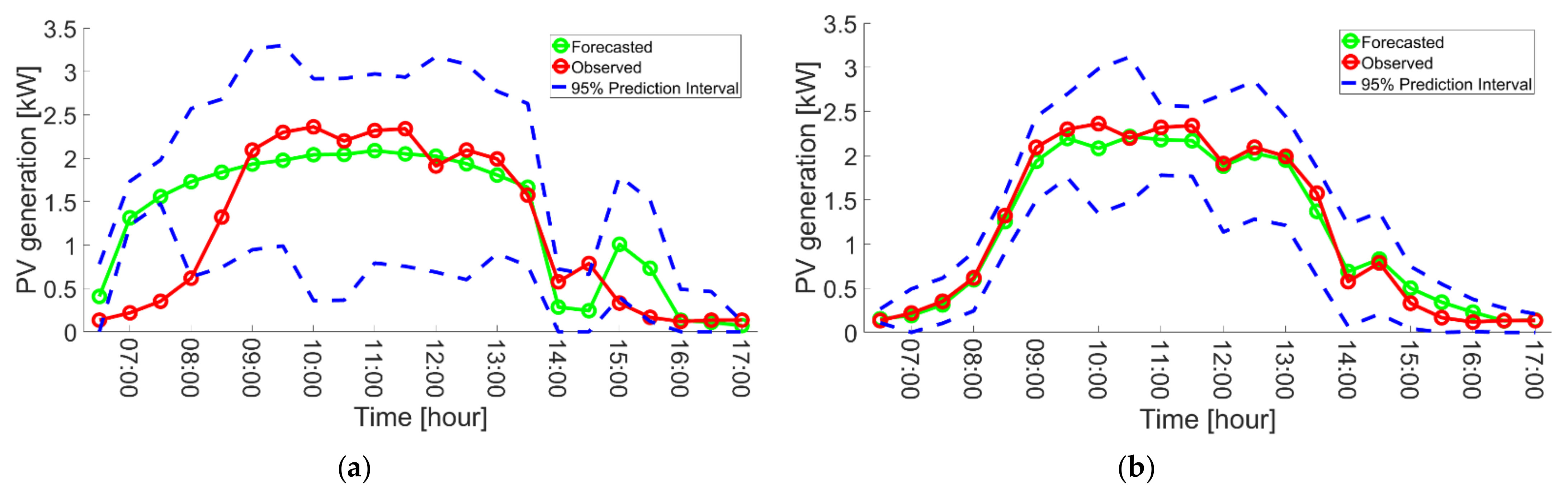
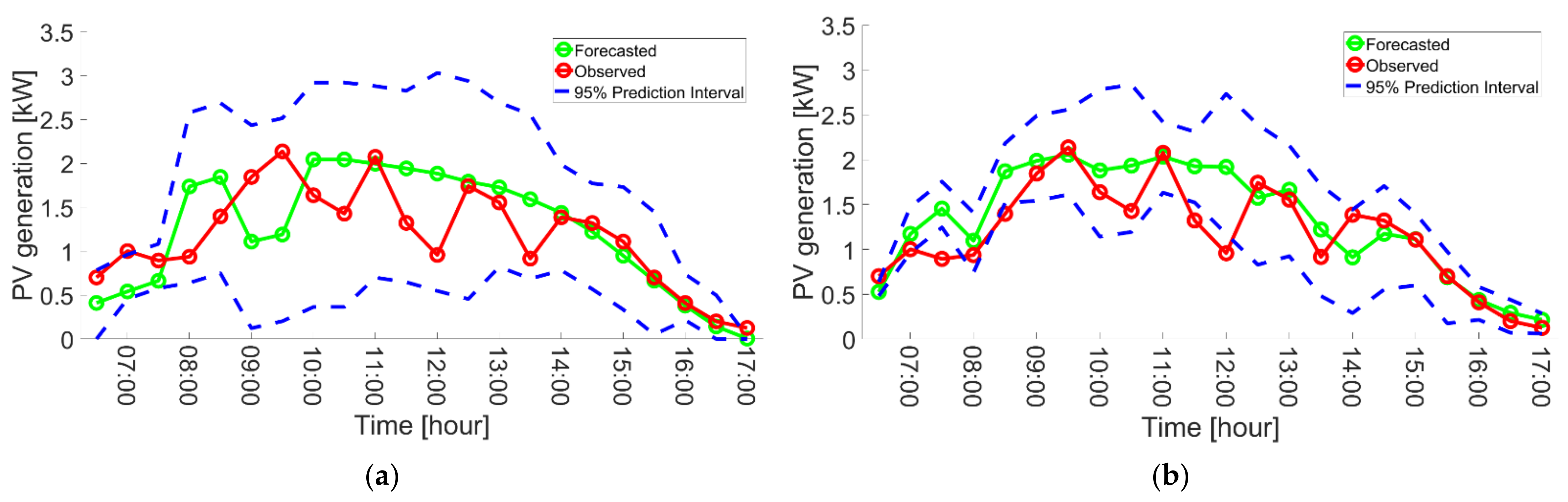
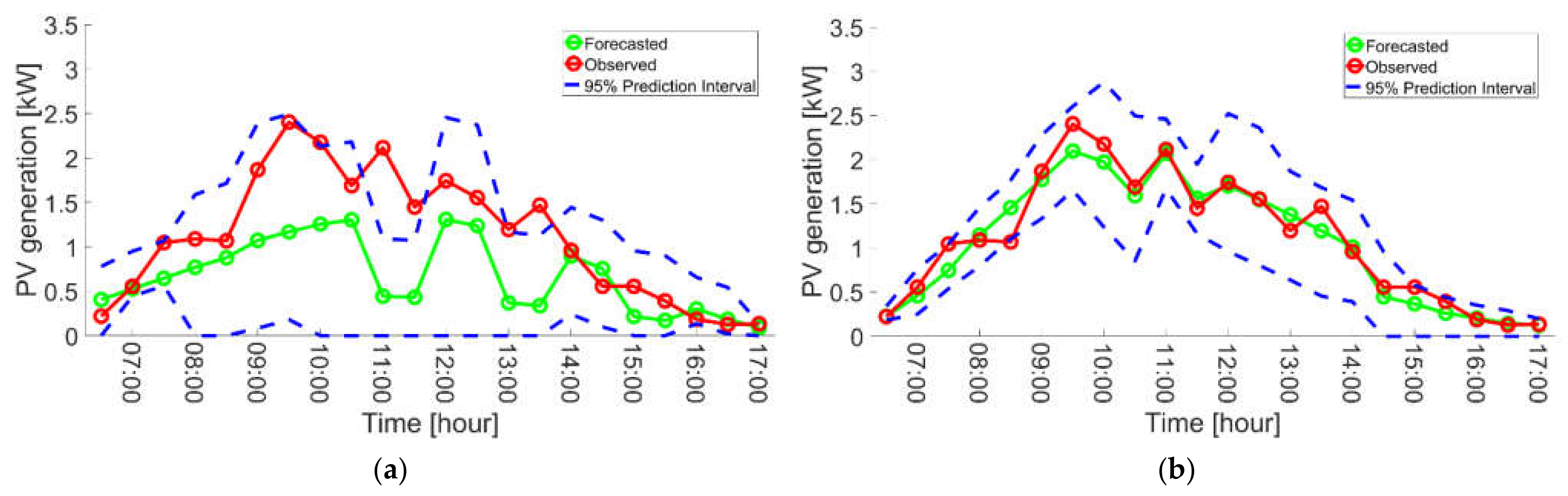
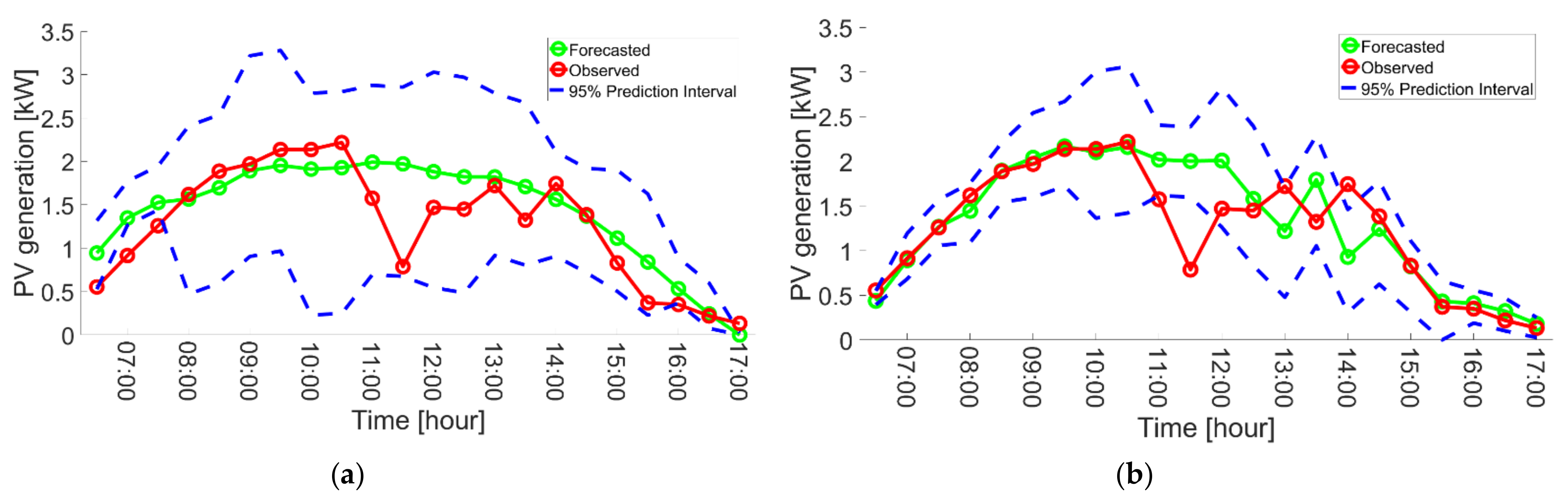
3.2.1. Forecast Result on the Best and Worst Day

Figure 7 shows the improvement in the forecasted results for PV (iii) on 11 July 2014. The rated power of PV (iii) is 3.42 kW. Figure 7a presents the day with the worst coverage rate among the 30 days using the single PV forecast model. Figure 7b was obtained using the multiple PV forecast model. The cover rate was improved from 72% to 100% using the multiple PV forecast model. In addition, the RMSE was reduced from 0.517 to 0.117 kW. However, in some cases, the PI cover rate is deteriorated by the multiple PV forecast model. Figure 8 shows the deteriorating of the forecasted results for PV (iii) on 15 July 2014. Figure 8a was obtained using the single PV forecast model. Figure 8b presents the day with the worst coverage rate among the 30 days using the multiple PV forecast model. Using the multiple PV forecast model, the cover rate deteriorated from 90 to 77%. However, the RMSE was reduced (improved) from 0.475 kW to 0.347 kW. The reason for the PI cover rate is that the PI width generated by the multiple PV forecast model is not narrower than that of the single PV forecast model.

As with the PI cover rate above, the RMSE calculated based on the single PV forecast model is also improved by the multiple PV forecast model. Figure 9 shows the improvement in the forecasted results for PV (iii) on 10 July 2014. Figure 9a shows the day with the worst RMSE of 30 days using the single PV forecast model. Figure 9b is obtained using the multiple PV forecast model for the same day. The average of the RMSE in a day was improved from 0.667 to 0.165 kW by the multiple PV forecast model. Figure 10 shows the deteriorating of the forecasted results for PV (iii) on 25 July 2014. Figure 10a was obtained using the single PV forecast model. Figure 10b presents the day with the worst RMSE of 30 days using the multiple PV forecast model. The RMSE slightly worsened from 0.372 to 0.382 kW using the multiple PV forecast model.

According to Figure 8 and Figure 10, the multiple PV forecast model is not always superior to the single PV forecast model for any case. Therefore, in the following subsection, we statistically analyze the forecast results to verify if the multiple PV forecast model is superior to the single PV forecast model for most cases.

3.2.2. Statistical Analysis of Forecast Result in the Whole Forecast Duration

Figure 11 shows a box plot of the cover rate of the prediction interval. In each box plot in Figure 11, the median of 30 days of forecasted result is represented by a red line. The edge of the box represents the 75th and 25th percentiles. Notches display the variability of the median between samples as confidence intervals. The width of a notch is computed such that boxes whose notches do not overlap have different medians at the 5% significance level. The significance level is based on a standard distribution assumption, but comparisons of medians are reasonably robust for other distributions [33].

Table 2. Summary of the multiple PVs forecast for 30 days.

		Cover Rate [%]		PI Width [kW]		MAPE [%]		RMSE [kW]
		Single	Multi	Single	Multi	Single	Multi	Single	Multi
PV (i)	M + 2σ	89.0	91.6	2.659	1.624	92.7	81.6	0.755	0.566
	Median (M)	86.4	86.4	2.578	1.581	67.1	60.9	0.684	0.479
	M − 2σ	83.8	81.2	2.497	1.537	41.5	40.3	0.614	0.392
PV (ii)	M + 2σ	87.0	94.8	1.442	0.797	69.5	24.8	0.386	0.196
	Median (M)	81.8	90.9	1.403	0.788	44.7	19.4	0.355	0.166
	M − 2σ	76.6	87.0	1.364	0.780	20.0	14.1	0.324	0.136
PV (iii)	M + 2σ	94.8	98.1	1.622	0.906	47.7	18.0	0.415	0.192
	Median (M)	90.9	95.5	1.574	0.887	36.6	15.1	0.377	0.153
	M − 2σ	87.0	92.8	1.525	0.867	25.6	12.1	0.339	0.113
PV (iv)	M + 2σ	90.3	93.5	7.196	4.086	53.1	28.2	1.794	0.939
	Median (M)	86.4	90.9	7.073	4.051	42.4	21.3	1.613	0.845
	M − 2σ	82.5	88.3	6.950	4.015	31.7	14.4	1.432	0.751
PV (v)	M + 2σ	96.1	90.3	1.232	0.897	63.6	39.3	0.365	0.216
	Median (M)	90.9	86.4	1.218	0.894	46.2	33.0	0.335	0.188
	M − 2σ	85.7	82.5	1.205	0.890	28.7	26.8	0.304	0.160

shows a summary of the boxplots from Figure 11, Figure 12, Figure 13 and Figure 14. In Table 2, the indicators that have improved compared to the single PV forecast model are highlighted.

Regarding the mean value of the PI cover rate, which is represented by the red line in Figure 11, the multiple PV forecast model outperforms the single PV forecast model in cases PV (ii), (iii), and (iv). PV (i) does not show significant differences between single and multiple PV forecast models. The weather in this season changes from west to east. The PV (i) does not change the result because the PV (i) is located on the west side among the five PVs and cannot obtain any information from the other PVs to improve the forecasting accuracy. PV (v) shows that the median of the PI cover rate decreases from 90.9 to 86.4% in the multiple PV forecast model, as shown in Table 2. Nevertheless, the minimum cover rate of the multiple PV forecast model is improved from the single PV forecast model, as indicated in the edge of the boxplot in Figure 11. PV (v) is located on the west side among the five PVs; therefore, the information from the far PVs such as PV (i) and PV (ii) is not variable to improve the forecast accuracy. Figure 12 shows the box plots of the PI width for the five PVs forecasted by the single PV and multiple PV forecast models. The PI width generated by multiple PV models was narrower in all PVs than in the single PV forecast model. As the PI width becomes narrower, the scheduling of the energy management systems becomes easier, and the scheduled operation can be realized with more probability. As shown in Figure 11, the PI cover rate was also improved or remained by the multiple PV forecast model. Regarding PV (ii), PV (iii), and PV (iv), Figure 11 and Figure 12 lead to an ideal result that the multiple PV forecast model simultaneously improves both the cover rate and PI width. The PV (ii), PV (iii), and PV (iv) are in the middle of the five PVs; therefore, they retrieve variable information from the surrounding PVs to improve forecast accuracy. With respect to PV (i) and PV (v), the PI width was improved. By contrast, the PI cover rate remained unchanged and valuable for energy management using ESSs or electric vehicle scheduling.

Figure 13 shows the boxplot of mean MAPE for five PV generations forecasted by the single and multiple PV forecast models, respectively. In all cases, the multiple PV forecast model shows a smaller MAPE than the single PV forecast model in terms of the mean. Figure 14 shows the boxplot of RMSE for five PV generations forecasted by the single and multiple PV forecast models, respectively. In all cases, the multiple PV forecast model showed a smaller RMSE than the single PV forecast model with respect to the mean. The results are shown in Figure 13 and Figure 14. The multiple PV forecast model improved the deterministic forecast accuracy in both MAPE and RMSE.

4. Conclusions

This study proposed a multiple PV forecast model based on ensemble forecasting for distributed PV in a specific area. The ensemble forecasting comprises naive Bayes classifier, NN, and LSTM with optimized weights using the PSO algorithm. In addition, error-based PI construction has also been proposed to convert deterministic forecasting into probabilistic forecasting. The proposed multiple PV forecast model utilizes the neighboring PV forecast result based on the proposed ensemble forecast method. As a result, the proposed multiple PV forecast model provides more reliable PIs for probabilistic forecasting and fewer errors for deterministic forecasting. The proposed multiple PV forecasting model is verified using five real PV generation data and climate data in the case study. As a result of continuous simulations with 30 days data, the RMSE, MAPE, PI cover rate, and PI width were improved by the multiple PV forecast model compared with the conventional single PV forecast model for all five PV cases. The advantage and the disadvantage are summarized as follows:

• Advantage:

The proposed two-step probabilistic forecast scheme can be applied to any machine learning algorithm. This study utilizes the ensemble forecasting model, which combines NN, naive Bayes classifier, and LSTM with optimized weights. The ensemble forecasting model is just one of the candidates to forecast PV generation on the proposed scheme.

• Disadvantage:

When we want to forecast a PV generation, the proposed two-step probabilistic forecast scheme utilized the surrounding PVs’ past data for training the forecasting model. This idea is based on the premise that these PVs are near, and the land is flat. However, the land that is not flat, and any obstacles such as trees, can change the tendency of the PV generations even they are near each other. In such cases, the proposed scheme is inefficient because the surrounding PVs’ information is not useful or is even noise to forecast the PV.

In future work, the multiple PV forecast model outperforms the single PV forecast model, but the effective way of selecting neighboring PVs should be investigated theoretically.

References

1. Haghdadi, N.; Bruce, A.; MaCgill, I.; Passey, R. Impact of Distributed Photovoltaic Systems on Zone Substation Peak Demand. IEEE Trans. Sustain. Energy 2018, 9, 621–629. [Google Scholar] [CrossRef]
2. Nagarajan, A.; Ayyanar, R. Design and Strategy for the Deployment of Energy Storage Systems in a Distribution Feeder with Penetration of Renewable Resources. IEEE Trans. Sustain. Energy 2015, 6, 1085–1092. [Google Scholar] [CrossRef]
3. Kodaira, D.; Jung, W.; Han, S. Optimal Energy Storage System Operation for Peak Reduction in a Distribution Network Using a Prediction Interval. IEEE Trans. Smart Grid 2020, 11, 2208–2217. [Google Scholar] [CrossRef]
4. Khosravi, A.; Nahavandi, S.; Creighton, D. Construction of optimal prediction intervals for load forecasting problems. IEEE Trans. Power Syst. 2010, 25, 1496–1503. [Google Scholar] [CrossRef] [Green Version]
5. Chai, S.; Xu, Z.; Jia, Y.; Wong, W.K. A Robust Spatiotemporal Forecasting Framework for Photovoltaic Generation. IEEE Trans. Smart Grid 2020, 11, 5370–5382. [Google Scholar] [CrossRef]
6. Agoua, X.G.; Girard, R.; Kariniotakis, G. Photovoltaic power forecasting: Assessment of the impact of multiple sources of spatio-temporal data on forecast accuracy. Energies 2021, 14, 1432. [Google Scholar] [CrossRef]
7. Agoua, X.G.; Girard, R.; Kariniotakis, G. Probabilistic Models for Spatio-Temporal Photovoltaic Power Forecasting. IEEE Trans. Sustain. Energy 2019, 10, 780–789. [Google Scholar] [CrossRef] [Green Version]
8. Lorenz, E.; Hurka, J.; Heinemann, D.; Beyer, H.G. Irradiance Forecasting for the Power Prediction of Grid-Connected Photovoltaic Systems. IEEE J. Sel. Top. Appl. Earth Obs. Remote Sens. 2009, 2, 2–10. [Google Scholar] [CrossRef]
9. Carrière, T.; Silva, R.A.e.; Zhuang, F.; Saint-Drenan, Y.-M.; Blanc, P. A New Approach for Satellite-Based Probabilistic Solar Forecasting with Cloud Motion Vectors. Energies 2021, 14, 4951. [Google Scholar] [CrossRef]
10. Pedro, H.T.C.; Larson, D.P.; Coimbra, C.F.M. A comprehensive dataset for the accelerated development and benchmarking of solar forecasting methods. J. Renew. Sustain. Energy 2019, 11, 036102. [Google Scholar] [CrossRef] [Green Version]
11. Mellit, A.; Pavan, A.M.; Ogliari, E.; Leva, S.; Lughi, V. Advanced methods for photovoltaic output power forecasting: A review. Appl. Sci. 2020, 10, 487. [Google Scholar] [CrossRef] [Green Version]
12. Pierro, M.; Bucci, F.; De Felice, M.; Maggioni, E.; Moser, D.; Perotto, A.; Spada, F.; Cornaro, C. Multi-Model Ensemble for day ahead prediction of photovoltaic power generation. Sol. Energy 2016, 134, 132–146. [Google Scholar] [CrossRef]
13. Chow, C.W.; Belongie, S.; Kleissl, J. Cloud motion and stability estimation for intra-hour solar forecasting. Sol. Energy 2015, 115, 645–655. [Google Scholar] [CrossRef]
14. Horn, B.K.P.; Schunck, B.G. Determining optical flow. Comput. Vis. 1981, 17, 185–203. [Google Scholar] [CrossRef] [Green Version]
15. Miyazaki, Y.; Kameda, Y.; Kondoh, J. A Power-Forecasting Method for Geographically Distributed PV Power Systems using Their Previous Datasets. Energies 2019, 12, 4815. [Google Scholar] [CrossRef] [Green Version]
16. Wen, H.; Du, Y.; Chen, X.; Lim, E.; Wen, H.; Jiang, L.; Xiang, W. Deep Learning Based Multistep Solar Forecasting for PV Ramp-Rate Control Using Sky Images. IEEE Trans. Ind. Inform. 2021, 17, 1397–1406. [Google Scholar] [CrossRef]
17. Al-Dahidi, S.; Ayadi, O.; Alrbai, M.; Adeeb, J. Ensemble approach of optimized artificial neural networks for solar photovoltaic power prediction. IEEE Access 2019, 7, 81741–81758. [Google Scholar] [CrossRef]
18. Hwang, J.T.G.; Ding, A.A. Prediction Intervals for Artificial Neural Networks. J. Am. Stat. Assoc. 1997, 92, 748–757. [Google Scholar] [CrossRef]
19. De Veaux, R.D.; Schumi, J.; Schweinsberg, J.; Ungar, L.H. Prediction intervals for neural networks via nonlinear regression. Technometrics 1998, 40, 273–282. [Google Scholar] [CrossRef]
20. MacKay, D.J.C. The Evidence Framework Applied to Classification Networks. Neural Comput. 1992, 4, 720–736. [Google Scholar] [CrossRef]
21. Nix, D.A.; Weigend, A.S. Estimating the mean and variance of the target probability distribution. IEEE Int. Conf. Neural Netw.-Conf. Proc. 1994, 1, 55–60. [Google Scholar]
22. Heskes, T. Practical confidence and prediction intervals. In Advances in Neural Information Processing Systems; MIT Press: Cambridge, MA, USA, 1997; pp. 176–182. [Google Scholar]
23. Khosravi, A.; Nahavandi, S.; Creighton, D.; Atiya, A.F. Comprehensive review of neural network-based prediction intervals and new advances. IEEE Trans. Neural Netw. 2011, 22, 1341–1356. [Google Scholar] [CrossRef] [PubMed]
24. Khosravi, A.; Nahavandi, S.; Creighton, D. Prediction Intervals for Short-Term Wind Farm Power Generation Forecasts. IEEE Trans. Sustain. Energy 2013, 4, 602–610. [Google Scholar] [CrossRef]
25. Ahmed, R.; Sreeram, V.; Mishra, Y.; Arif, M.D. A review and evaluation of the state-of-the-art in PV solar power forecasting: Techniques and optimization. Renew. Sustain. Energy Rev. 2020, 124, 109792. [Google Scholar] [CrossRef]
26. Park, S.; Han, S.; Son, Y. Demand power forecasting with data mining method in smart grid. In Proceedings of the 2017 IEEE Innovative Smart Grid Technologies-Asia (ISGT-Asia), Auckland, New Zealand, 4–7 December 2017; pp. 1–6. [Google Scholar]
27. Function Fitting Neural Network—MATLAB & Simulink—MathWorks. 2021. Available online: https://www.mathworks.com/help/deeplearning/ref/fitnet.html;jsessionid=aefb10cd790c33d77ace7a56705a (accessed on 26 October 2021).
28. Long Short-Term Memory Networks—MATLAB & Simulink—MathWorks. Available online: https://jp.mathworks.com/help/deeplearning/ug/long-short-term-memory-networks.html?lang=en (accessed on 2 September 2021).
29. Algorithm Implementation Codes on GitHub. Available online: https://github.com/daisukekodaira/Improving-Forecast-Reliability-for-Geographically-Distributed-Photovoltaic-Generations (accessed on 26 October 2021).
30. Agyeman, K.A.; Kim, G.; Jo, H.; Park, S.; Han, S. An Ensemble Stochastic Forecasting Framework for Variable Distributed Demand Loads. Energies 2020, 13, 2658. [Google Scholar] [CrossRef]
31. Møller, M.F. A scaled conjugate gradient algorithm for fast supervised learning. Neural Netw. 1993, 6, 525–533. [Google Scholar] [CrossRef]
32. Kim, T.; Ko, W.; Kim, J. Analysis and impact evaluation of missing data imputation in day-ahead PV generation forecasting. Appl. Sci. 2019, 9, 204. [Google Scholar] [CrossRef] [Green Version]
33. MathWorks. Visualize Summary Statistics with Box Plot. 2021. Available online: https://jp.mathworks.com/help/stats/boxplot.html?lang=en (accessed on 23 August 2021).
Figure 1. Configuration of the single and multiple PV forecast model.
Energies 14 07340 g001
Figure 2. Configuration of an ensemble forecasting model.
Energies 14 07340 g002
Figure 3. Configuration of an ensemble forecasting model.
Energies 14 07340 g003
Figure 4. Data configuration; long-term past data for training and error validation. Forecast data for forecasting unknown PV generations.
Energies 14 07340 g004
Figure 5. Forecasted and observed PV generation on the i-th day.
Energies 14 07340 g005
Figure 6. Location of the PV systems to be forecasted in Japan.
Energies 14 07340 g006
Figure 7. Improvement of forecasted PV generation for PV (iii) on 11 July 2014. The day has the worst PI coverage rate by the single PV forecast model among 30 days. (a) Single PV forecast model for PV (iii) (Cover rate = 72%). (b) Multiple PV forecast model for PV (iii) (Cover rate = 100%).
Energies 14 07340 g007
Figure 8. Deteriorating of forecasted PV generation for PV (iii) on 15 July 2014. The day has the worst PI coverage rate by the multiple PV forecast model among 30 days. (a) Single PV forecast model for PV (iii) (Cover rate = 90%). (b) Multiple PV forecast model for PV (iii) (Cover rate = 77%).
Energies 14 07340 g008
Figure 9. Improvement of forecasted PV generation for PV (iii) on 10 July 2014; the worst RMSE by the single PV forecast model among 30 days performances. (a) Single PV forecast model for PV (iii) (RMSE = 0.667 kw). (b) Multiple PV forecast model for PV (iii) (RMSE = 0.165 kw).
Energies 14 07340 g009
Figure 10. Deteriorating of forecasted PV generation for PV (iii) on 25 July 2014; the worst RMSE by the multiple PV forecast model among 30 days performances. (a) Single PV forecast model for PV (iii) (RMSE = 0.372 kw). (b) Multiple PV forecast model for PV (iii) (RMSE = 0.382 kw).
Energies 14 07340 g010
Figure 11. Box plot for prediction interval cover rate; Single PV vs. Multiple PV forecast model at five locations.
Energies 14 07340 g011
Figure 12. Box plot of prediction interval width; Single PV vs. Multiple PV forecast model at five locations.
Energies 14 07340 g012
Figure 13. Box plot for mean absolute percentage error (MAPE); Single PV vs. Multiple PV forecast model at five locations.
Energies 14 07340 g013
Figure 14. Box plot for root mean square error (RMSE); Single PV vs. Multiple PV forecast model at five locations.
Energies 14 07340 g014