Green Growth in the OECD Countries: A Multivariate Analytical Approach

Abstract

Green growth is about merging environmental and social protection with economic growth. The OECD countries follow the progress toward greening though a set of indicators. The aim of the study is to analyze the condition and development of the OECD countries using a set of green growth indicators. The univariate and multivariate statistical approach was used to identify the main features of green growth development in two time spans. The achieved success of the OECD countries toward the green growth was measured from period 1 (years 2000–2009) to period 2 (years 2010–2019). For stimulant indicators, an increase was achieved, while for the destimulant variables, a decrease was reached between the analyzed periods. CO₂ productivity increased by more than 31%, material productivity by 25%, and the energy productivity by nearly 21%. From the ecological point of view, a positive sign was achieved by an intensive increase of the percentage of municipal waste treatment by recycling or composting. The real GDP increased between periods in each of the OECD countries, except in Greece. The destimulant indicators decreased over time. The mortality declined by about 20% from exposure to ambient PM_2.5 and thus the welfare costs of premature death from exposure to PM_2.5 also declined. The decline of the mean population exposure to PM_2.5 by 12.5% on average for the OECD countries is a positive signal for environmental protection and public health of the OECD population. Some uncertainty exists as the municipal waste generated per capita decreased only slightly by 2%.

1. Introduction

After the great recession that occurred between 2007 and 2009 and led to a global recession in 2009 [1], countries were seeking ways to restore their economies. OECD countries and their partner economies were looking for a framework that would not only help to achieve economic recovery, but would also secure environmentally and socially sustainable growth [2]. The Declaration of Green Growth adopted at the OECD Meeting of the Council at Ministerial Level in 2009 supports the efforts towards green growth strategies, acknowledging that green and growth can go hand-in-hand. In 2011, OECD launched the Green Growth Strategy, in which it characterized sustainable growth that can generate new economic opportunities by fostering investment and innovation and thus ensure the protection of natural assets, their resources, and services for future generations [3].

Green growth merges environmental and social protection with the allowance for economic growth, thus achieving sustainable development. It fosters the creation and adoption of new development models, while effectively reducing pressure on the environment [4,5]. This concept is also more attractive to policy and decision makers, while traditional environmental protection approaches are often linked to economic slowdown and are seen as barriers to development [4].

On the other hand, the transition of economies to green growth is not pain-free [6]. Some authors argue that it is not possible to achieve green growth without harming the economic growth, or to respect sustainability if the intensive consumption of goods continues to foster economic growth [7,8,9]. The assumption of green growth that economies will be able to maintain or even increase their economic activity ecologically by using new technologies that drastically cut carbon emissions can be seen as a problem [10]. Some authors have suggested that, in order to foster green growth, carbon emission programs need to be supplemented by other policies and international pressure and they must not be pursued at the expense of social equality and welfare [6], while others concluded that green growth objectives are misguided and need to be replaced [5]. Contrary to these opinions, the European Union (EU) built on the green growth with its European Green Deal introduced in December 2019.

EU aims to be the first climate neutral continent by transforming all its economy sectors to meet its climate targets in a way that is fair, cost effective, and competitive [11]. While recovering from the COVID-19 pandemic, around 600 billion euros from the union’s recovery plan will be used for this transformation in order to counter climate change and environmental degradation [12].

Returning to the basis of green growth, its aims cannot be achieved from day to day. Thus, the OECD introduced green growth indicators, which build on the analysis of central elements of green growth [13]. Each of these central elements can be measured by various indicators and focus on the following aspects: the socio-economic characteristics of growth, the environmental and resource productivity of the economy, the natural asset base of the economy, the environmental dimension of quality of life, and the economic opportunities from innovation and effective policies [13].

Many experts closely link a green economy to a dependency of economic development from natural environmental factors [14,15,16,17,18]. Green economies initiate an implementation of new technologies that increase natural capital and decrease environmental risks [19,20,21]. The pandemic crisis has brought new perspectives on the research of green growth concepts. Recently, green growth concepts have been used to explain regional, national, and international strategies that support the economic recovery of countries from recession caused by the pandemic crisis. Also, green economies are closely related to social area, and they includes economic, legislative, and structural opportunities [22,23,24]. Many countries create plans for effective and sustainable production and consumption while they prepare adequate legislative frameworks for a green economy. These plans are interconnected with the plans for the effective use of resources [25,26,27]. The integrated approaches that identify market opportunities and evaluate legislative initiatives within a green economy, while linking to modern tax systems, access to information about hazardous substances, the standard setting of waste minimization, and so on, are being increasingly promoted. Globalization changes significantly influence the changes of green economies’ interventions [28,29]. The pandemic crisis, with both economic and financial crises, caused aggressive changes in the ways of life. The most considerable part of the interventions focused on the protection of human lives and economies, while the issues of waste economy became secondary [30,31,32,33]. The role of the public policies, i.e., education, research, and communication dimensions, has been significantly increasing recently. Sharing the principles, so-called best practices, and the formation of international research teams is very important in order to create and verify those best practices in green economies [31,34,35,36]. Effective political tools are necessary within the public policies that aim at reaching economic recovery and the growth of environmental and social sustainability [30,34]. The increased consumption of resources and energy and the increased production of waste that has a negative impact on the environment influence those indicators to a great extent. Significantly higher economic growth should be generated by obtaining a higher economic value from a limited number of natural resources [32,37]. It is assumed that once the economic processes are more effective, there will be an implementation of new technologies and an ability to create cost savings. In the future, there will be pressure for the creation of strong links between environmental protection, industrial policy and competitiveness policy, research, innovations, and the education system. This would enable the formation of new conceptual relations between green economies, green growth, and sustainable development at the national and international level. Green economies will always create new opportunities for green and a sustainable development to enter public policies and the space for the development of new partnerships that will be based on co-operation and new sustainable business models [33,38,39].

Green growth is a global priority strategy that is implemented to respond to climate change [40], and the results are investigated by governments, academia, and international organizations. The results show that green growth in uneven in the EU or OECD countries and the green growth indicators vary between countries [41]. For boosting this positive kind of growth, a rise in R&D subsidies is needed to redirect growth from polluting to clean economic movements [42] and to focus on renewable energy [43].

Economic development positively influences green growth [44], and therefore the government’s priority should be on the conjunction of greening of the economy and its sustainable development [45]. Political support on various levels and central coordination, and cooperation of all public authorities and private environments will also be very important.

2. Materials and Methods

The set of green growth indicators used for the analysis of the status of 38 OECD countries were downloaded from the OECD.Stat database [46]. The database is freely accessible and comprises data and metadata not only for the OECD countries but also for some non-member economies. The OECD green growth indicators enable the monitoring of progress towards objectives of environmental and resource productivity, the natural asset base, the environmental dimension of quality of life, economic opportunities, and policy responses [2,3,13]. Some of the green growth indicators belong to the set of indicators that measure the distance to the sustainable development indicators [47]. The 2030 Agenda of Sustainable Development is in the interest of every human being, policy makers, countries, and their regions as it is a broad and ambitious plan of action for people, the planet, and prosperity [47,48]. Governments across the world are trying to adopt measures for greener growth and to underline their ambition for the greening of their economies [4], but some researchers states that the economic growth will hardly be achievable by fulfilling the targets for green growth [8,9,49]. For analysis of a solo indicator, the univariate statistical approach was used as recommended [50,51], and the variables were characterized by its average level, minimum, maximum, standard deviation, and coefficient of variation (CV). The CV, as a relative measure of variability, is suitable to follow the variability in different time dimensions and it allows for the comparison of the variability for different indicators. The CV belongs to the so-called sigma convergence coefficients [52,53]. Convergence is an often-discussed topic for countries joined into an international platform, and it is a subject of regional convergence in a specific country [54,55,56]. The linear association between a pair of variables was detected using Pearson’s correlation coefficient. In addition to univariate statistical methods, in this paper, multidimensional methods for assessing the state of the OECD countries were applied. From a multidimensional point of view, the cluster analysis and the principal component analysis (PCA) were applied to the selected set of indicators. The selected indicators are part of the OCED green growth indicators. Cluster analysis is a useful tool that attempts to identify structures within the selected dataset. For grouping objects, in our case OECD countries, into clusters, different algorithms and methods were used. These methods did not make any distinction between independent or dependent variables, and they discovered a system of organizing observations into groups where members of a group share specific properties in common [57,58]. Cluster analysis (CA) identifies a homogenous group of objects (in our case, objects are the OECD countries), where objects are alike within the same cluster and are dissimilar to the objects in other different clusters. According to the mentioned information, we can expect that the degree of association between two objects is maximal if they belong to the same group and minimal otherwise [59]. CA is a special technique that organizes the observed data or cases into two or more homogenous groups. The advantage of CA is that it does not assume any prior information about the classification of an object into a specific cluster. Different measures can be used to identify the distance between objects for specific data types and several different hierarchical or non-hierarchical methods were used to determine which clusters should be joined at each stage, for example, the furthest neighbor method, nearest neighbor method, average linkage method, centroid method, k-mean clustering method, and Ward’s method [59,60,61]. Clusters can play an important role in supporting green growth strategy and sustainable development processes [62]. For clustering, all 38 OECD countries were used as objects and selected variables from the green growth database were used as indicators. The collinearity of selected variables was checked since strong linear association is a typical issue for multivariate statistical analysis. It was therefore necessary to include the analysis of linear association and to deal with the problem of a strong correlation between the selected indicators. The principal component analysis was chosen to resolve the issue of a high linear association between the variables. PCA belongs to dimension reduction methods. It makes it possible to create a smaller number of linear combinations of selected variables that should account for most of the variance in a correlation matrix pattern [63,64]. PCA serves to identify a minimum number of factors that will account for maximum variance in the analyzed dataset. Therefore, PCA is a dimension reduction technique that is used to reduce a large group of variables to a smaller set of uncorrelated principal components. PCA initially creates the same number of components as is the number of original variables but usually only a few of the “most important” components are used for the next step of analysis. The most important components were used in the study to realize the cluster analysis. The first principal component accounts for the highest variability in the dataset and each consecutive component accounts for as much of the remaining variability as possible [63,64,65]. Therefore, for the analysis it is necessary to take only the first m eigenvectors that explain a desired threshold of the total variability. The cumulative percent of variance explained, as a criterion for solving the number of components, should be at least 70% [66,67]. The next criterion for determination of the number of components is the Kaiser criterion. The criterion indicates that the minimum variance explained by the factor should be equal to or greater than 1, which means it should be greater than the variance of a single observed indicator [67,68]. PCA is a helpful analytical approach for the reduction of the input data dimensions and for the creation of a “new” uncorrelated dataset for the consequent multivariate analysis.

3. Results

The analysis of the selected indicators for the OECD countries was done in two periods. The first period (period 1) includes variables for the time span from 2000 to 2009 and the second period (period 2) consists of indicators for the time span between 2010 and 2019. For each indicator, an average value was calculated for period 1 and period 2; this average was calculated for every OECD member state. In case the values of some indicators were not yet published for 2019, the average of the variables was calculated according to the availability. From the OECD green growth database [2,3,13], a selection of variables was realized to create a statistical file suitable for analytical purposes. The indicators were selected from groups that capture the main features of green growth, namely environmental and resource productivity of the economy and the environmental dimension of quality of life, and from the socio-economic context of the OECD countries. Some of the selected indicators are part of the Sustainable Development Goals. The condition of the selection of variables was also the ability to indicate whether the indicator is a stimulant or destimulant. The following indicators of green growth were included in our study:

• x₁ CO₂ productivity, GDP per unit of energy-related CO₂ emissions;
• x₂ Energy productivity, GDP per unit of total primary energy supply (TPES);
• x₃ Material productivity, GDP per unit of domestic material consumption (DMC);
• x₄ Municipal waste recycled or composted, % of waste treated;
• x₅ Renewable energy supply, % of TPES;
• x₆ Population with access to improved drinking water sources in %;
• x₇ Population with access to improved sanitation, % of total population;
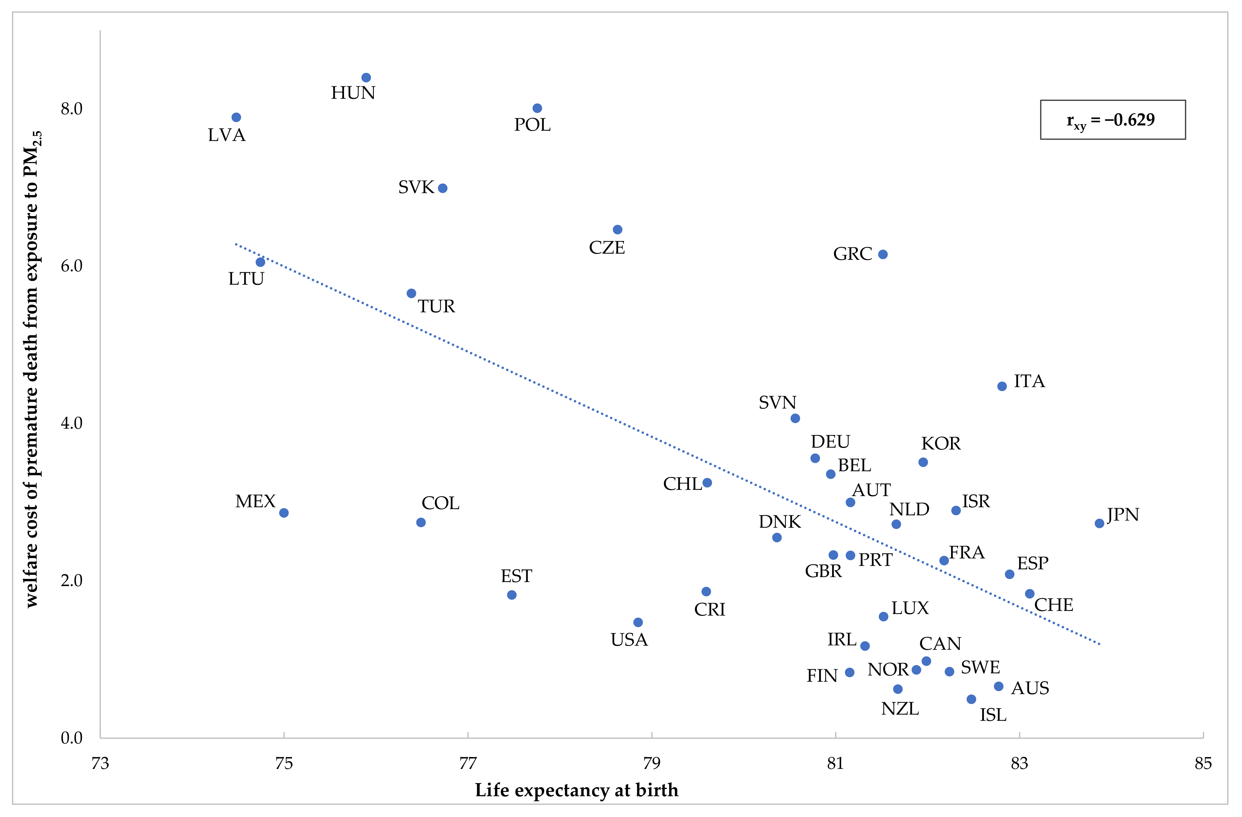
• x₈ Life expectancy at birth;
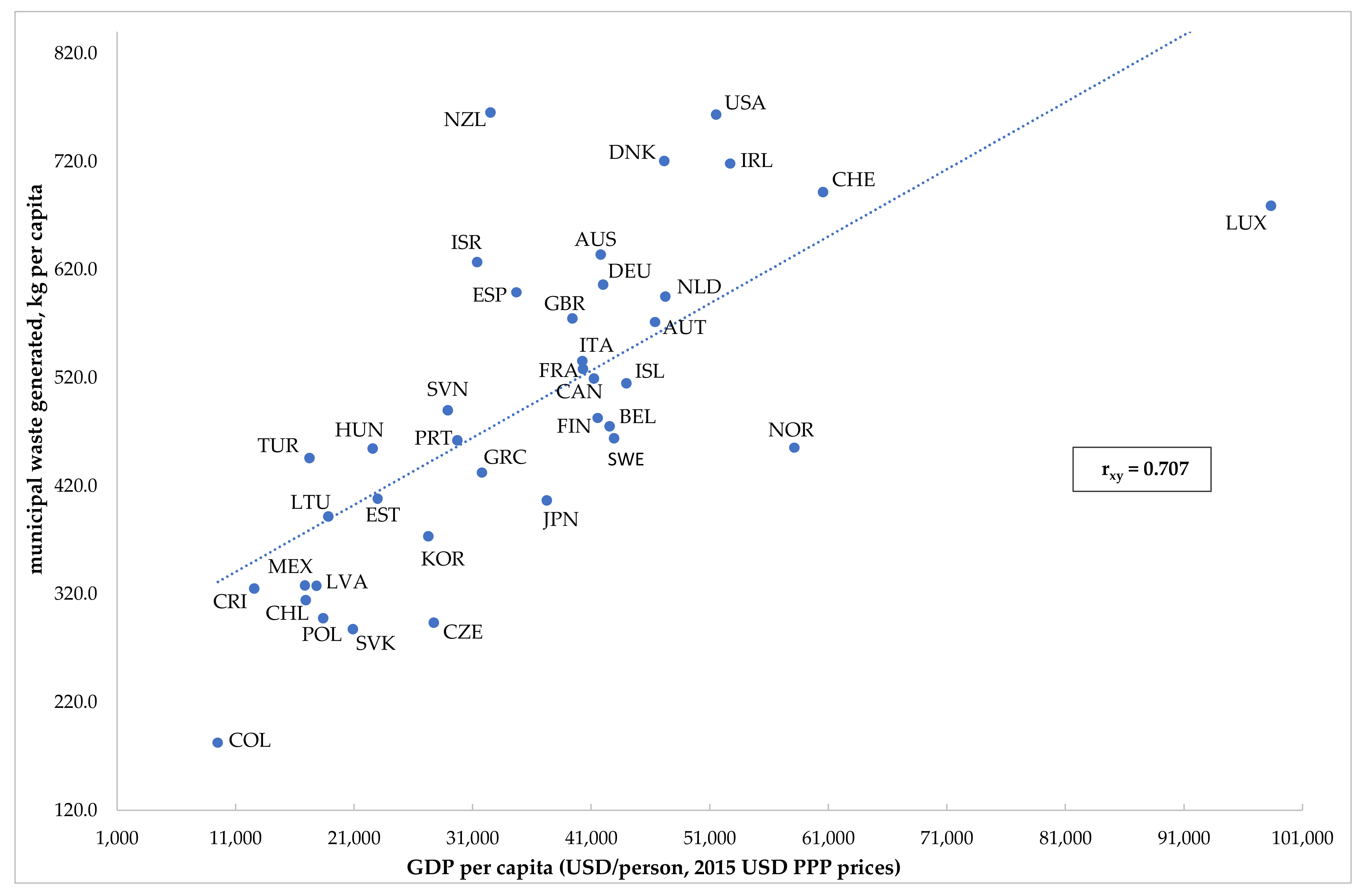
• x₉ Real GDP per capita;
• x₁₀ Real GDP, index 2000 = 100;
• x₁₁ Energy intensity, TPES per capita;
• x₁₂ Municipal waste generated, kg per capita;
• x₁₃ Mean population exposure to PM_2.5;
• x₁₄ Mortality from exposure to ambient PM_2.5;
• x₁₅ Welfare cost of premature death from exposure to ambient PM_2.5.

The indicator x₁ is calculated as real GDP generated per unit of CO₂ emitted in USD/kg. The GDP is expressed at constant USD prices (2015) in purchasing power parity (PPP). The energy productivity (x₂) is measured as GDP per unit of TPES in USD/toe (tonne of oil equivalent). The energy productivity and energy intensity also reflect the structural and climatic factors. The non-energy material productivity (x₃) is calculated as GDP generated per unit of DMC, per unit of material consumed in USD/kg. Indicator x₄ is measured as the percentage of municipal waste recycled or composted from all waste treated. The variable x₅ is calculated as the percentage of renewable energy in the total primary energy supply. The indicator x₆ represents the percentage of the population using improved drinking water. The improved water sources should be available when needed and free of chemical and fecal contamination. The percentage of population with access to improved sanitation (x₇) reflects the share of the total population using improved sanitation and a basic handwashing facility. The life expectancy at birth (x₈) is the average number of years a newborn child can expect to live if mortality patterns throughout his or her life stay unchanged. Real GDP per capita (x₉) is measured at constant 2015 USD PPP prices in USD/person. The real growth of the GDP (x₁₀) is calculated in the form of base year index with a base period in year 2000. The indicator x₁₁ is measured as the total primary energy supply per capita and expressed in toe per person. The variable x₁₂ measures the volume of municipal waste generated per person in kg. From the environmental quality of life, the exposure to fine particulate matter was of interest in this paper. Indicator x₁₃ is calculated as the mean annual outdoor PM_2.5 concentration weighted by population living in the area and is expressed in micrograms per cubic meter (μg/m₃). The previous indicator is closely related to the indicators x₁₄ and x₁₅. The mortality from exposure to ambient PM_2.5 is calculated in death per million inhabitants. The welfare costs of premature mortality from exposure to PM_2.5 represents the cost estimates of premature mortalities and are compared to the gross domestic product as percentage points of GDP equivalent.

3.1. Status and Development of Indicators

The analyzed indicators are either stimulants or destimulants. Ten variables belong to stimulants, i.e., the indicators x₁–x₁₀, and five indicators belong to destimulants, i.e., x₁₁–x₁₅. The indicators where the maximalization is positive are stimulants and the variables where the minimalization is positively rated are destimulants [69,70,71].

In

Table 1. Relative and absolute change of the indicators between period 1 and period 2.

Variable	Period 1	Period 2	Relative Change, %	Absolute Change
X1	4.8	6.3	31.3	1.5
X2	9681.0	11,696.4	20.8	2015.4
X3	2.8	3.5	25.0	0.7
X4	24.7	33.1	34.0	8.4
X5	14.7	19.2	30.6	4.5
X6	91.5	94.6	3.4	3.1
X7	79.0	84.3	6.7	5.3
X8	77.9	80.2	3.0	2.3
X9	35,622.4	40,027.3	12.4	4404.9
X10	125.2	161.6	29.1	36.4
X11	4.1	4.0	−2.4	−0.1
X12	493.3	482.7	−2.1	−10.6
X13	16.0	14.0	−12.5	−2.0
X14	384.1	309.8	−19.3	−74.3
X15	4.0	3.2	−20.0	−0.8

Source: OECD.Stat database [20]—our calculations based on OECD database.

, the mean values of the analyzed variables for the OECD countries are presented for both periods. In addition, the table includes the rate of change of indicators between these periods. In the case of the favorable development of stimulant variables, their increase is expected. Conversely, for a favorable change of destimulant variables, a decrease is considered positively.

The first 10 indicators are stimulants, and according to the rate of change (in percent) the development of these indicators can be rated positively. The average CO₂ productivity for the OECD countries in the second period (average for 2010–2019) jumped by 31.3% compared to the average for the first period (average for 2000–2009). Similarly high was the gain of the energy productivity, which increased by 20.8%, and the material productivity, which grew by 25%. The percentage of municipal waste recycled or composted jumped by 34%. The increase of the renewable energy supply was higher than 30%. The only moderate rates of change were for indicators x₆, x₇, and x₈. It seems that these indicators had very high levels in most of the OECD countries in the first period and therefore a rate of change was not possible for these countries in the second period. A very good example is the share of population with access to improved drinking water sources. This share was already 100% in some countries in the first period, so it is not possible to increase this proportion in the future. Also, in the case of LE at birth, only a moderate increase is expected over time, and due to the COVID-19 situation it is possible that it will decrease. The destimulant variables changed positively overtime as they decreased in the analyzed time span. Also, a moderate decrease of energy intensity or a moderate decline of municipal waste generated per capita is a good signal for future green growth. The drop of the mean population exposure to PM_2.5, as high as 12.5%, must be rated very positively. This decline positively influenced the death rates and welfare costs of premature death from exposure to ambient PM_2.5. The mortality from exposure to ambient PM_2.5 shrank by more than 19% and the welfare costs of premature death declined by 20%; these results are very good news for the populations living in the OECD countries.

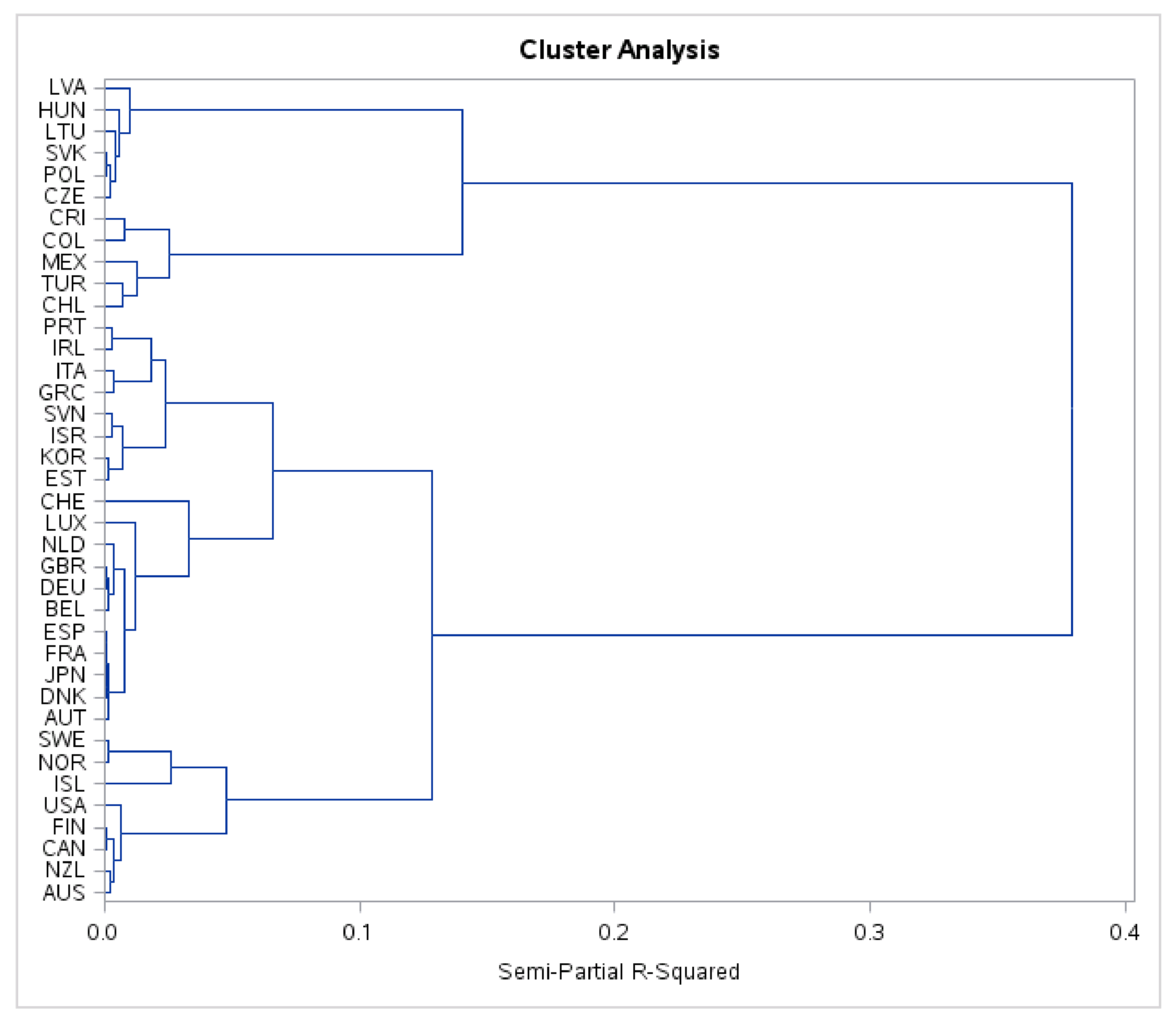
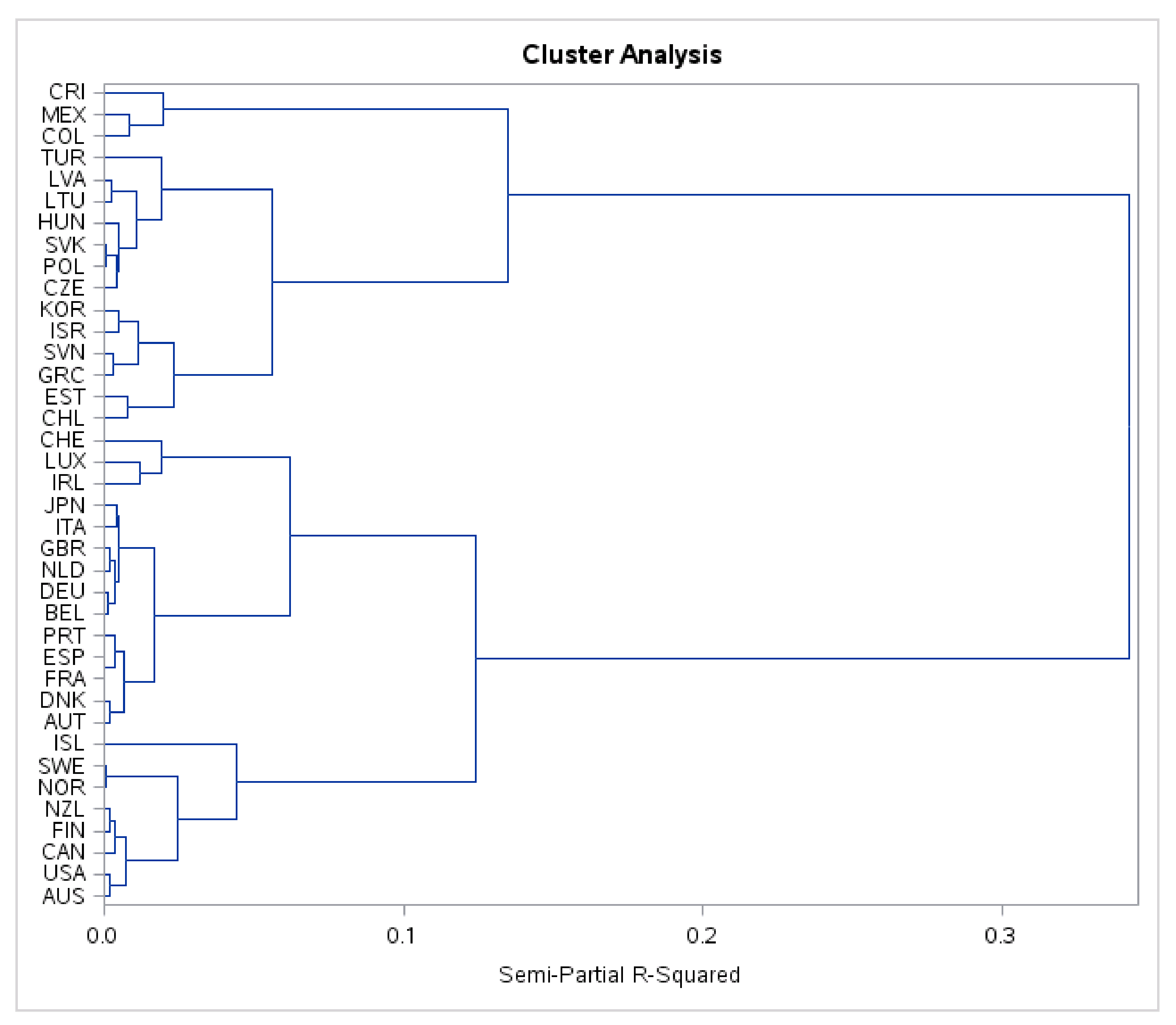
3.2. Cluster Analysis

Cluster analysis of the OECD countries was performed in two periods for segmentation reasons. The Ward’s minimum variance method was used for clustering [72]. The selected hierarchical cluster analysis expects uncorrelated variables. Due to this presumption, a correlation analysis was realized and, in case of a strong correlation between the input variables, the principal component analysis was used to calculate the principal components. The main principal components were than selected for the cluster analysis and the clustering was done using the noncorrelated main principals.

3.2.1. Cluster Analysis of the OECD Countries in Period 1

The correlation between some pairs of the input indicators was statistically significant at the probability value (p value) of 0.05. In

Table 2. Pearson’s correlation coefficients of the variables in period 1.

Variables	X1	X2	X3	X4	X5	X6	X7	X8	X9	X10	X11	X12	X13	X14	X15
X1	1
X2	0.608	1
X3	0.238	0.276	1
X4	0.079	0.037	0.462	1
X5	0.499	−0.102	−0.235	−0.149	1
X6	−0.086	−0.089	0.267	0.490	−0.048	1
X7	−0.264	−0.244	0.413	0.559	−0.402	0.499	1
X8	0.180	0.090	0.376	0.590	0.091	0.517	0.250	1
X9	0.107	0.106	0.556	0.700	−0.075	0.466	0.442	0.586	1
X10	−0.094	−0.215	−0.463	−0.513	0.194	−0.109	−0.327	−0.585	−0.497	1
X11	−0.172	−0.551	0.195	0.426	0.309	0.382	0.274	0.463	0.652	−0.218	1
X12	−0.011	0.164	0.298	0.626	−0.138	0.315	0.430	0.533	0.707	−0.490	0.417	1
X13	−0.063	0.252	−0.045	−0.436	−0.295	−0.365	−0.293	−0.470	−0.536	0.331	−0.622	−0.551	1
X14	−0.265	−0.060	0.020	−0.317	−0.363	−0.130	0.275	−0.601	−0.339	0.285	−0.396	−0.372	0.568	1
X15	−0.264	−0.075	−0.035	−0.374	−0.333	−0.168	0.227	−0.642	−0.401	0.332	−0.425	−0.418	0.582	0.997	1

Source: OECD.Stat database [51]—our calculations based on OECD database.

, the associations measured by the Pearson’s correlation coefficient r_xy in absolute values higher than 0.60 are marked in bold. The highest positive correlation (r_xy = 0.997) was between the mortality from exposure to ambient PM_2.5 and the welfare cost of premature death from this exposure in GDP equivalent. Both indicators are overlapping, and it is unsurprising that the linear relationship between these variables was so high and positive. The association between the GDP per capita and the municipal waste generated per capita (r_xy = 0.707) was also very high and positive, which means that in countries with a high GDP per capita, higher waste generated per person is expected and vice versa. The association of these indicators is graphically shown in Figure 1, where countries with lower GDP per capita and lower municipal waste generation are positioned in the bottom left corner, while countries with higher GDP per person and higher waste generation per capita are positioned in the upper right corner. The high positive correlation between the municipal waste generated per capita and the percentage of municipal waste recycled or composted (r_xy = 0.626) can be positively rated. Thus, in countries with a high generation of municipal waste, the percentage of recycling or composting of this waste is also high. The correlations between the following indicators were also high and position: CO₂ productivity and energy productivity, GDP per capita and percentage of recycled or composted municipal waste, and real GDP per capita and energy intensity. The correlation between life expectancy at birth and mortality from exposure to ambient PM_2.5 and between life expectancy at birth and the welfare cost of premature death from exposure to ambient PM_2.5 were high but negative. As was mentioned above, high correlations are not desirable for the chosen clustering method and therefore the PCA analysis helped to create new variables, principal components, that were uncorrelated with each other.

According to the selection criteria, components with eigenvalues equal to or greater than 1 were selected and by the second condition the components that cumulatively explain more than 70% of the total variance were used for the next stage of analysis. The PCA of the 15 original indicators is presented in

Table 3. Principal component analysis eigenvalues of correlation matrix in period 1.

Eigenvalues of the Correlation Matrix
	Eigenvalue	Difference	Proportion	Cumulative
1	5.620	2.859	0.375	0.375
2	2.760	0.584	0.184	0.559
3	2.177	1.090	0.145	0.704
4	1.087	0.301	0.072	0.776
5	0.785	0.107	0.052	0.829
6	0.679	0.127	0.045	0.874
7	0.552	0.170	0.037	0.911
8	0.382	0.049	0.026	0.936
9	0.333	0.091	0.022	0.958
10	0.243	0.075	0.016	0.975
11	0.167	0.057	0.011	0.986
12	0.111	0.035	0.007	0.993
13	0.075	0.047	0.005	0.998
14	0.028	0.028	0.002	1.000
15	0.000		0.000	1.000

Source: OECD.Stat database [51]—our calculations based on OECD database.

. Four main components have eigenvalues higher than 1 and they explain in total nearly 78% of the variability in the original data set. The cluster analysis was realized using these four principal components, which reduced the complexity of the original 15 indicators, and solved the problem of the high and statistically significant correlation between some pairs of indicators.

The graphical summary of the cluster analysis for the first period is presented in Figure 2. The parsing of the dendrogram, the classification tree, allowed the OECD countries to be split into six clusters.

The main characters of the clusters were evaluated by the cluster centroids presented in

Table 4. Cluster centroids of OECD countries in period 1.

Clusters of OECD Countries	Cluster 1	Cluster 2	Cluster 3	Cluster 4	Cluster 5	Cluster 6
Number of countries	5	3	11	8	5	6
X1	3.1	7.3	5.4	4.0	6.3	3.8
X2	6592.2	7040.0	11,141.1	10,408.4	12,589.3	7505.0
X3	1.7	2.9	4.3	2.5	1.8	2.1
X4	30.3	33.9	42.3	22.5	1.2	5.8
X5	16.4	50.9	7.6	7.5	24.0	10.1
X6	94.0	97.4	98.1	93.9	75.4	84.7
X7	82.6	73.5	94.4	79.6	36.2	85.4
X8	79.5	80.5	79.7	78.3	75.5	73.6
X9	41,714.3	48,335.1	48,713.2	33,119.3	14,614.0	21,034.0
X10	122.1	122.7	113.2	125.6	135.4	142.1
X11	6.5	8.0	4.5	3.3	1.2	2.9
X12	633.0	478.3	586.3	505.9	319.3	342.2
X13	8.1	8.1	14.5	17.4	23.9	20.8
X14	147.5	140.9	357.2	410.7	268.7	813.3
X15	1.4	1.3	3.5	4.3	3.0	8.8

Source: OECD.Stat database [20]—our calculations based on OECD database.

.

Cluster 1 (five countries: Australia, New Zealand, Canada, Finland, and the United States)

The countries in the first cluster achieved the lowest value of the production-based CO₂ productivity, and this fact must be rated negatively for the countries grouped together into this cluster. The energy and material productivity for this cluster were also the lowest. The municipal waste generated per capita was the highest among the clusters while the percentage of recycled or composted waste was positioned in the middle of all the clusters. The lowest mean population exposure to PM_2.5 and the related indicators, i.e., very low mortality rates from exposure to ambient PM_2.5 and welfare costs of premature death from this exposure, were positive.

Cluster 2 (three countries: Iceland, Norway, and Sweden)

Countries grouped together in the second cluster were similar to the countries in the first cluster with a low energy productivity and material productivity, but had a higher CO₂ productivity. They are successful in terms of low mean population exposure to PM_2.5 and related indicators. The waste generated per capita was positive in the middle of the clusters and was combined with the second highest percentage of municipal waste treaded by recycling or composting. These countries also achieved the highest life expectancies at birth, and a very high percentage of their population has access to improved drinking water sources. Their living standard as measured by GDP per capita was the second highest among the clusters.

Cluster 3 (11 countries: Austria, Denmark, Japan, France, Spain, Belgium, Germany, the United Kingdom, the Netherlands, Luxembourg, and Switzerland).

Cluster three includes the most countries. Altogether 11, development countries joined together and had the highest GDP per capita and very high CO₂, energy, and material productivities. The cumulative real GDP growth between 2000 and 2009 was only 13.2%, which makes the expectation about a convergence of the OECD countries in terms of GDP per capita possible. Unfortunately, most of the development countries produced the largest amount of municipal waste per capita, but on the other hand these countries also achieved the highest percentage of recycled or composted waste from the total waste treated. These countries compensate for the high production of municipal waste by the recycling or composting of generated waste. The renewable energy supply compared to that of the countries in the second cluster was exceedingly low. Hopefully, the development countries will, in the near future, invest more into the production of renewable energy, which is beneficial to nature and the environment. As expected in countries with a high living standard, this cluster had the highest percentage of population with access to improved drinking water sources (98.1%) and improved sanitation (94.4%). Their LE at birth was the second highest. Other analyzed variables were in the middle position among the clusters.

Cluster 4 (eight countries: Estonia, Korea, Israel, Slovenia, Greece, Italy, Ireland, and Portugal)

In the fourth cluster, European countries joined together with Israel and Korea. These countries produced the third largest amount of municipal waste per capita, but the percentage of waste recycled or composted was quite low (only 22.5%), which means that it was nearly 20 percentage points lower compared with the results for countries in cluster 3. The waste generation and the low percentage of waste recycling or composting is a problem for the countries in cluster 4. The percentage of renewable energy supply was also negatively rated, as it commonly reached only 7.5% for these countries. For comparison, it was as high as 50.9% in cluster 2. The cluster had the second highest mortality from exposure to ambient PM_2.5 and the welfare cost of premature death from this exposure.

Cluster 5 (five countries: Chile, Turkey, Mexico, Colombia, and Costa Rica)

Cluster 5 is composed of less developed OECD countries that reached the lowest value of GDP per capita and the lowest percentage of population with access to improved drinking water sources (75.4%) and improved sanitation (only 36.2%). The real GDP cumulative growth was, however, higher than 35%. These countries reached the second lowest level of LE at birth. From the green growth perspective, the highest CO₂ and energy productivity and the second largest percentage of renewable energy supply must be rated very positively. The production of municipal waste compared with the more developed countries was at a low level, but the percentage of recycling or composting of the waste was the lowest. According to the expectations, as the living standard increases in these countries, so too will the generation of waste per capita. Therefore, the percentage of waste recycling or composting should be increased from only 1.2%; otherwise, these countries will suffer from problems with waste generation.

Cluster 6 (six countries: Czechia, Poland, Slovak Republic, Lithuania, Hungary, and Latvia).

The European post-communist countries joined together into cluster 6. Lower CO₂, energy, and material productivities were typical for these countries. They had the second lowest GDP per capita level, which was compensated with the highest real rate of GDP growth. This fact creates the precondition of convergence of the OECD countries in terms of the GDP per capita indicator as this indicator is suitable for the analysis of the convergence processes [73]. These countries’ municipal waste generation per capita was the second lowest, but the percentage of recycling or composting of the waste was also very low. The lowest value of LE at birth, the very high mean population exposure to PM_2.5, the extremely high mortality from exposure to ambient PM_2.5, and the resulting highest value of welfare cost of premature death from this exposure must be evaluated very negatively for the European post-communist countries.

3.2.2. Cluster Analysis of the OECD Countries in Period 2

The linear relationship between some pairs of the input indicators was also statistically significant in the second time span. In

Table 5. Pearson’s correlation coefficients of the variables in period 2.

Variables	X1	X2	X3	X4	X5	X6	X7	X8	X9	X10	X11	X12	X13	X14	X15
X1	1
X2	0.565	1
X3	0.118	0.311	1
X4	0.107	−0.004	0.469	1
X5	0.454	−0.212	−0.409	−0.147	1
X6	−0.032	−0.128	0.211	0.449	0.043	1
X7	−0.161	−0.163	0.424	0.665	−0.278	0.622	1
X8	0.141	0.042	0.437	0.490	0.052	0.582	0.394	1
X9	0.198	0.163	0.461	0.641	−0.058	0.437	0.461	0.538	1
X10	−0.026	0.056	−0.408	−0.403	0.062	−0.135	−0.390	−0.523	−0.250	1
X11	−0.078	−0.591	0.003	0.270	0.488	0.310	0.196	0.363	0.469	−0.100	1
X12	0.184	0.204	0.221	0.523	0.056	0.364	0.403	0.509	0.692	−0.370	0.318	1
X13	−0.186	0.152	−0.005	−0.424	−0.315	−0.372	−0.358	−0.424	−0.533	0.412	−0.481	−0.547	1
X14	−0.236	0.008	−0.016	−0.185	−0.322	−0.124	0.124	−0.598	−0.431	0.202	−0.419	−0.446	0.607	1
X15	−0.233	−0.004	−0.067	−0.235	−0.291	−0.151	0.084	−0.629	−0.473	0.228	−0.428	−0.476	0.608	0.998	1

Source: OECD.Stat database [51]—our calculations based on OECD database.

, the highest correlations are marked in bold. The highest positive correlation was between the mortality from exposure to ambient PM_2.5 and the welfare cost of premature death from this exposure in GDP equivalent. The association between the population with access to improved sanitation and percentage of waste recycled or composted (r_xy = 0.665) and between the municipal waste generated per capita and GDP per capita (r_xy = 0.692) was very intensive. The association between GDP per capita and the percentage of municipal waste recycled or composted (r_xy = 0.641) was also very high and positive, which means that in countries with a higher living standard the percentage of treated waste by recycling or composting was also high. The correlation coefficient between the GDP per capita and the generation of municipal waste per capita was very strong. The correlations between the mean population exposure to PM_2.5 and mortality from exposure to ambient PM_2.5 or the welfare cost of premature death from this exposure was also positive and significant. The association between LE at birth and the mortality from exposure to ambient PM_2.5 (r_xy = −0.598) and between the LE at birth and the welfare cost of premature death from exposure to ambient PM_2.5 (r_xy = −0.629) was negative. The results of the association measures were very similar to those in period 1. The linear relationship between indicators x₈ and x₁₅ is graphically presented in Figure 3. From this figure, it is clear that a strong negative association exists between both variables. The countries with lower life expectancies but higher welfare costs of premature death from exposure to ambient PM_2.5 (GDP equivalent) are located in the upper left corner; these countries were mostly European post-communist countries. Countries with higher life expectancy at birth and lower welfare costs of premature death are positioned in the bottom right corner; these countries are the most developed OECD countries.

As in the first period, due to a high linear relationship between some pairs of analyzed variables, the clustering procedure was realized using the main principal components. Components with eigenvalues equal to or greater than 1 were selected, and by the second condition the components that cumulatively accounted for more than 70% of the total variance were used for the cluster analysis. The PCA of the 15 original indicators is presented in

Table 6. Principle component analysis—Eigenvalues of correlation matrix in period 2.

Eigenvalues of the Correlation Matrix
	Eigenvalue	Difference	Proportion	Cumulative
1	5.386	2.714	0.359	0.359
2	2.672	0.604	0.178	0.537
3	2.069	0.926	0.138	0.675
4	1.143	0.250	0.076	0.751
5	0.893	0.128	0.060	0.811
6	0.764	0.052	0.051	0.862
7	0.712	0.272	0.048	0.909
8	0.440	0.098	0.029	0.939
9	0.342	0.151	0.023	0.961
10	0.191	0.035	0.013	0.974
11	0.156	0.051	0.010	0.985
12	0.105	0.017	0.007	0.992
13	0.088	0.050	0.006	0.998
14	0.038	0.037	0.003	1.000
15	0.000		0.000	1.000

Source: OECD.Stat database [20]—our calculations based on OECD database.

. Four main components have eigenvalues higher than 1, and they explain more than 75% of the variability in the original data set. The cluster analysis was realized using these four main principal components, which reduced the complexity of the original data set, and solved the problem of the high and statistically significant linear relationship between some of the indicators.

The dendrogram of the cluster analysis for the second period is presented in Figure 4. According to the presented tree, i.e., dendrogram, the OECD countries were split into seven clusters.

The main characteristics of the clusters are presented using the cluster centroids in

Table 7. Cluster centroids of OECD countries in period 2.

Clusters of OECD Countries	Cluster 1	Cluster 2	Cluster 3	Cluster 4	Cluster 5	Cluster 6	Cluster 7
Number of countries	7	1	11	3	6	7	3
X1	5.9	8.1	6.5	9.6	4.1	5.5	8.1
X2	8383.0	2838.0	12,988.6	19,802.5	10,041.8	10,874.7	14,762.3
X3	2.3	2.5	5.0	5.6	3.2	2.5	2.5
X4	37.6	27.6	43.8	46.6	29.0	22.7	3.7
X5	26.3	88.9	14.2	11.1	12.5	15.2	28.3
X6	98.6	98.0	98.0	97.3	97.4	92.1	69.2
X7	85.6	73.7	94.0	90.8	87.5	85.5	33.9
X8	81.5	82.5	81.7	82.0	80.6	76.4	77.0
X9	48,148.0	49,238.1	42,876.5	77,999.2	31,199.9	27,799.7	15,775.3
X10	149.2	176.0	126.3	181.8	173.7	198.1	185.4
X11	5.9	17.4	3.4	4.3	3.4	2.7	1.1
X12	569.1	555.1	521.1	645.8	447.0	366.0	297.2
X13	6.8	6.6	12.4	10.2	18.8	19.1	21.3
X14	94.6	52.2	289.5	169.7	346.1	658.3	227.2
X15	0.9	0.5	2.9	1.5	3.6	7.1	2.5

Source: OECD.Stat database [51]—our calculations based on OECD database.

.

Cluster 1 (seven countries: Australia, United States, Canada, Finland, New Zealand, Norway, and Sweden)

The first cluster is composed of seven countries, from which five were in the same cluster in period 1. Norway and Sweden were added to the original five countries from the first period. The countries in this cluster typically had a very high GDP per capita level, high LE at birth, and the highest percentage of the population with access to improved drinking water sources. These developed countries had a very low mean population exposure to PM_2.5 combined with very low mortality rates from this exposure. As a negative sign of development in these countries, the municipal waste generation per capita was the second highest among the clusters. Surprisingly, the CO₂ and material productivity were in middle levels, while the energy productivity and energy intensity had the second worst values among the clusters.

Cluster 2 (solo country: Iceland)

In the second period, one solo cluster was created. The values of indicators in Iceland were so different to the values of the other OECD countries that Iceland was separated from the other countries. The renewable energy supply reached an extremely high level of 88.9%. In Iceland, we can see a high CO₂ productivity, but the lowest energy productivity and a very low material productivity. The second highest level of GDP per capita among the clusters created an expectation for a high percentage of recycling or composting of municipal waste, but this level only reached 27.6%. Iceland reached an extremely high energy intensity level. Iceland’s mean population exposure to PM_2.5, the mortality from exposure to ambient PM_2.5, and the welfare cost of premature death from this exposure had the lowest values among the clusters.

Cluster 3 (11 countries: Austria, Denmark, France, Spain, Portugal, Belgium, Germany, the Netherlands, United Kingdom, Italy, and Japan)

Cluster 3 had a very similar composition in both periods. The only change is that in this second period Portugal and Italy were also placed into the cluster three, while Luxembourg and Switzerland were relocated into cluster 4. These European countries and Japan have a high GDP per capita, but the lowest real growth of GDP. The material productivity was the second highest, while energy intensity of these countries was relatively low. The higher waste generation per capita was associated with a very high percentage of waste recycling or composting. Other indicators of cluster 3 were set in the middle among the created clusters.

Cluster 4 (three countries: Ireland, Luxembourg, and Switzerland)

The OECD countries with a very high living standard were joined together in cluster 4. They reached the highest GDP per capita combined with a very high real growth of GDP. The CO₂, energy, and material productivity of these countries was the highest among all the clusters and must be rated very positively. The highest generation of municipal waste per capita must be rated negatively, but on the other hand cluster 3’s percentage of recycled or composted waste was among the highest. The mean population exposure to PM_2.5 and the mortality from exposure to ambient PM_2.5 were low. Surprisingly, the lowest percentage of renewable energy supply was reached in this cluster.

Cluster 5 (six countries: Chile, Estonia, Greece, Slovenia, Israel, and Korea)

The countries in cluster 5 had the lowest CO₂ productivity, but also low energy and material productivity. The renewable energy supply was only at 12.5%. The mean population exposure to PM_2.5 was higher which resulted in the higher mortality and welfare cost of premature death from this exposure. The energy intensity per capita was on the lower end.

Cluster 6 (seven countries: Czechia, Poland, Slovak Republic, Hungary, Lithuania, Latvia, and Turkey)

All the European post-communist countries that were together in period 1 were also put together in the second period. These countries were also joined by Turkey in the second period. The countries in cluster six reached the second lowest GDP per capita and the highest real GDP growth. This fact creates the chance of a convergence of the living standard among the OECD countries. The LE at birth was only 76.4%, the worst value. The energy intensity per capita was low, which is a positive feature of countries in cluster 6. Unfortunately, the low material and CO₂ productivity must be rated negatively. Even worse was the situation with the extremely high level of mortality from exposure to ambient PM_2.5, while the mean population exposure to PM_2.5 was the second highest. The municipal waste generation was still not very high, but it was combined with the second lowest level of waste recycling or composting.

Cluster 7 (three countries: Colombia, Mexico, and Costa Rica)

The less developed OECD countries joined together and created the cluster seven. These countries had the lowest level of GDP per capita and the second largest real GDP growth. They commonly achieved a high CO₂ and energy productivity. They had the lowest levels of population with access to improved drinking water sources (69.2%) and population with access to improved sanitation (33.9%). The LE at birth was a bit higher than in cluster 6, but still low when compared with other clusters. This cluster having the highest mean population exposure to PM_2.5 must be negatively rated. The energy intensity per capita and the generation of municipal waste per capita were among the lowest values, but as the living standard will increase in the future, it is expected that the energy intensity and the generation of waste will rise. This cluster had the lowest percentage of waste recycling or composting (only 3.7%), which must also be rated negatively.

4. Discussion

The green growth strategy should help to recover the economies with a focus on environmental and social sustainable growth. The OECD countries are concentrating on their green growth strategy [2,3,13] while the EU countries are paying attention to the European green deal [11,12]. The green economy provides an economic approach to sustainable growth with a focus on employment, investments, and skills [74]. The main directions of green growth in the OECD countries are measured by indicators that cover the main aspects of economic, environmental, and social lives. These aspects include environmental and resource productivity, the natural asset base, the environmental dimension of quality of life or economic opportunities, and policy response. To be able to assess the state and development of the OECD green growth initiative, a set of fifteen variables were created. Some of the variables were stimulants and some of them were destimulants. The positive development of a stimulant indicator shows green growth, while a positive development of a destimulant indicator shows a decline.

The cluster analysis of OECD countries performed in the first period split the member states into six clusters. Cluster 1 (5 countries), cluster 2 (3 countries), and cluster 3 (11 countries) represent the most developed countries with a high living standard, highest GDP per capita levels, and a moderate cumulative real GDP growth rate. These countries (especially in cluster 1) had a high municipal waste generation per capita that was compensated by a high percentage of waste recycling or composting. Their mean population exposure to PM_2.5, the mortality from exposure to ambient PM_2.5, and the welfare cost of premature death from this exposure were low in clusters 1 and 2 but a bit higher in cluster 3. Between these clusters, there are differences in terms of productivity and energy intensity measures (indicators x₁, x₂, x₃, and x₁₁). The percentage of renewable energy supply was the highest in the second cluster. The countries in cluster 4 had a lower living standard compared with clusters 1–3 but a higher standard than countries in clusters 5 and 6. They achieved the third highest energy and material productivities. The high mortality rate from exposure to ambient PM2.5 and the high welfare cost of premature death from this exposure must be negatively rated. The countries with a lower GDP per capita but a high cumulative real GDP growth rate joined clusters 5 and 6. The high GDP growth rate makes the convergence process of the GDP per capita real. These countries recorded a high mean population exposure to PM_2.5 that was combined, especially in the case of cluster 6, with a high mortality rate from exposure to ambient PM_2.5 and also a high welfare cost of premature death from this exposure. These countries had a lower municipal waste generation per capita but the percentage of waste recycling or composting for these countries was very low. The biggest difference between the last two clusters is in the energy productivity and CO₂ productivity levels. In future, it is expected that the living standard will improve in the countries in clusters 5 and 6, but according to a high positive correlation between waste generation and GDP per capita, the municipal waste generation will also increase. Therefore, the low percentage of waste recycling or composting can cause a problem with waste landfilling. The high mean population exposure to ambient PM_2.5 is also problematic. The countries in the last two clusters reached the lowest proportions of population with access to improved drinking water sources and improved sanitation and the lowest life expectancies at birth.

The cluster analysis in the second period enabled the OECD member states to be split into seven clusters. Clusters one and two together consist of the same countries as in the first period. The only difference is that seven countries were joined in cluster 1 and cluster 2 was a solo cluster with only one country: Iceland. One of the reasons contributing to Iceland being in a solo cluster is the extremely high value of the indicator x₅, which represents the percentage of the renewable energy supply of TPES. The ratio was nearly 89%. Iceland also had the lowest values for mean population exposure to PM_2.5, the mortality from exposure to ambient PM_2.5, and the welfare cost of premature death from this exposure. The living standard in this solo country is high and the real growth rate of the GDP per capita was also relatively high. Iceland can be rated as a successful country in meeting the green growth strategy. The countries in the first cluster had very low levels of variable x₁₃, x₁₄, and x₁₅, and the best position of variable x₆. Other indicators were in the middle between the clusters. Nearly all the countries that joined together into cluster 3 in the first period also joined together in the second period. The countries in cluster 3 were very successful in securing their population with access to improved drinking water sources and improved sanitation. These countries had the second highest material productivity and second highest percentage of municipal waste treated by recycling or composting. The high GDP per capita was associated with the lowest cumulative real growth rate of GDP. The fourth cluster can be rated as the best one according to the highest values of CO₂, energy, and material productivities, the highest percentage of treated waste by recycling or composting, and the highest real GDP per capita values. There are two indicators that these countries should improve on their road toward a green strategy: decreasing the highest value of municipal waste generation and increasing the lowest proportion of renewable energy supply. Cluster 5 consists of countries that were joined together in the first period, plus Chile. These countries insufficiently meet the objectives of the strategy in term of CO₂, energy productivities, renewable energy supply, and the mean population exposure to PM_2.5 and their related indicators. The European post-communist countries and Turkey joined cluster 6. These countries reached the worst values for indicators that negatively influence the public health of the population. These indicators include the mean population exposure to PM_2.5, the resulting highest mortality from exposure to ambient PM_2.5, and the highest welfare cost of premature death from this exposure, while the LE at birth was the lowest among the created clusters. The living standard measured by GDP per capita was still low but was compensated by the highest cumulative real GDP growth rate. The last cluster represents the less developed OECD countries according to the lowest GDP per capita level. These countries have reached an extremely low percentage of the population with access to improved sanitation, the lowest proportion of population with access to improved drinking water sources, and the lowest percentage of treated waste by recycling or composting at only 3.7%.

5. Conclusions

The OECD countries, according to the analyzed indicators in the study, were successful in meeting the goals of the green growth strategy. Between two time spans, a positive development was achieved for the stimulant and for the destimulant variables. We are pleased to state that all the selected variables developed in a proper way over the analyzed time span. The first period represents the average values of the variables between 2000 and 2009 and the second period represents the average values of indicators between 2010 and 2019. The productivity indicators (CO₂ productivity, energy productivity, material productivity) increased rapidly from the first to the second period. The percentage of municipal waste that was treated by recycling or composting increased by 34% (an increase of 8.4 p.p.) in the second period compared with the first period. Also significant was the increase of the renewable energy supply that relatively changed by 30.6% (an increase of 4.5 p.p.). The real GDP per capita increased by more than 12%. The other stimulant variables increased only moderately, but it is necessary to state that these indicators corresponded to the populations with access to improved drinking water sources, the populations with access to improved sanitation, and the life expectancy at birth. The increase is not possible for some countries, since in some countries the percentage of population with access to improved drinking water sources was already equal to 100% in period 1 (Luxembourg, the United Kingdom, the Netherlands). If the percentage is equal to 100%, no improvement for these countries is possible, and this fact influences the overall increase for the OCED countries. The increase of the percentage of population with access to improved sanitation was very moderate. The explanation for this is similar to the explanation of the moderate growth of indicator x₆. In the first period, the percentage of the population with access to improved sanitation was higher than 98% in Finland, Switzerland, and Japan. The destimulant indicators decrease over time, a positive sign of green development. The mean population exposure to PM_2.5 decreased by 12.5%, while the mortality from exposure to ambient PM_2.5 shrank by more than 19%, and the welfare cost of premature death from this exposure declined by 20%. All these results are very important and positive for public health and environmental issues. More activity from populations and governments is needed in the areas of energy intensity and the generation of municipal waste. These indicators changed only moderately. Unfortunately, in period 2 there were countries where the municipal waste generation per capita was higher than 700 kg (Switzerland, USA, Denmark). According to the findings, a positive and strong linear relationship exists between the waste generation per capita and the percentage of municipal waste recycling or composting. Therefore, in countries with high municipal waste generation where the treatment of waste is properly addressed, it does not create such a high pressure on environmental burdens.

The cluster analysis helped to detect countries with a similar condition of analyzed indicators, which creates the possibility of putting in place concrete measures for countries in a cluster to improve their situation in regard to green growth strategy. The most developed countries should focus their efforts on reducing municipal waste generation, as these countries produce a large amount of waste per capita. On the other hand, the less developed OECD countries should pay more attention to creating conditions for waste recycling or composting because their rates of recycling or composting are low. These efforts can be positive for green development even in cases where the living standard will increase, which is associated with an increase of municipal waste generation. The European post-communist countries must focus on cleaner environments and a reduction of population exposure to PM_2.5 due to the fact that in these countries the mortality from exposure to ambient PM_2.5 is dramatically high. The decline of the population exposure and the decline of the mortality from exposure to ambient PM_2.5 will result in a decline of their high welfare cost for premature death from exposure to PM_2.5. The economic costs of air pollution are high; thus, improving air quality have economic benefits along with an enormous effect on human health. For less developed countries, an important increase in their green effort will be associated with investments into the access of better drinking water sources and into the access to improved sanitation. Post-communist countries in particular should also concentrate on better usage of energy and material consumption that will result in higher energy and/or material productivity levels. These recommendations come from the results of cluster analysis. The cluster analysis enabled the identification of countries with similar states of selected indicators, which helped to discover the main features and the main pros and cons of the countries that were joined in a specific cluster.

Green growth should be of interest of governments, institutions, and human beings as it creates preconditions for “healthy economic growth” and an increase in quality of life and the health of the population and subsequent generations.

References

1. IMF. World Economic Outlook—April 2009: Crisis and Recovery. Available online: https://www.imf.org/en/Publications/WEO/Issues/2016/12/31/Crisis-and-Recovery (accessed on 15 July 2021).
2. OECD. Towards Green Growth? Tracking Progress; OECD Publishing, OECD Green Growth Studies: Paris, France, 2015. [Google Scholar]
3. OECD. Towards Green Growth; OECD Publishing, OECD Green Growth Studies: Paris, France, 2011. [Google Scholar]
4. Capasso, M.; Hansen, T.; Heiberg, J.; Klitkou, A.; Steen, M. Green growth—A synthesis of scientific findings. Technol. Forecast. Soc. Chang. 2019, 146, 390–402. [Google Scholar] [CrossRef]
5. Kasztelan, A. Green growth, green economy and sustainable development: Terminological and relational discourse. Prague Econ. Pap. 2017, 26, 487–499. [Google Scholar] [CrossRef] [Green Version]
6. Gough, I. Can growth be green? Int. J. Health Serv. 2015, 45, 443–452. [Google Scholar] [CrossRef] [Green Version]
7. Fernandes, C.I.; Veiga, P.M.; Ferreira, J.J.M.; Hughes, M. Green growth versus economic growth: Do sustainable technology transfer and innovations lead to an imperfect choice? Bus. Strategy Environ. 2021, 30, 2021–2037. [Google Scholar] [CrossRef]
8. Hickel, J.; Kallis, G. Is green growth possible? New Political Econ. 2019, 25, 469–486. [Google Scholar] [CrossRef]
9. Dercon, S. Is green growth good for the poor? World Bank Res. Obs. 2014, 29, 163–185. [Google Scholar] [CrossRef]
10. Ossewaarde, M.; Ossewaarde-Lowtoo, R. The EU’s Green deal: A third Alternative to Green Growth and Degrowth? Sustainability 2020, 12, 9825. [Google Scholar] [CrossRef]
11. European Commission. Delivering the European Green Deal. Available online: https://ec.europa.eu/info/strategy/priorities-2019-2024/european-green-deal/delivering-european-green-deal_en (accessed on 15 July 2021).
12. European Commission. A European Green Deal. Available online: https://ec.europa.eu/info/strategy/priorities-2019-2024/european-green-deal_en (accessed on 17 July 2021).
13. OECD. Green Growth Indicators 2017; OECD Publishing: Paris, France, 2017. [Google Scholar]
14. Fanta, M. Water management in the Czech Republic: Transformation, restructuralization, and comparison of the current state of the branch with the state in 1993. Littera Scr. 2019, 12, 1–12. [Google Scholar]
15. Kabourková, K.; Stuchlý, J. Structural development of utilised agricultural area in EU countries subsidy policy of the Czech Republic. Literra Scr. 2019, 12, 1–17. [Google Scholar] [CrossRef] [PubMed]
16. Kmecová, I.; Tlustý, M.; Velková, V. The analysis of legal environment and administrative burden od SMEs as an obstacle to business. Literra Scr. 2020, 13, 135–152. [Google Scholar]
17. Vochozka, M.; Maroušková, A.; Šuleř, P. Economic, environmental and moral acceptance of renewable energy: A case study-the agricultural biogas plant at Pěčín. In Science and Engineering Ethics; Springer: Dordrecht, The Netherlands, 2017; Volume 24, pp. 299–305. [Google Scholar]
18. Maroušek, J.; Rowland, Z.; Valášková, K.; Král, P. Techno-economic assessment of potato waste management in developing economies. In Clean Technologies and Environmental Policy; Springer: New York, NJ, USA, 2020; Volume 22, pp. 937–944. ISSN 1618-954X. [Google Scholar] [CrossRef]
19. Škapa, S.; Vochozka, M. Towards Higher Moral and Economic Goals in Renewable Energy. In Science and Engineering Ethics; Springer: Dordrecht, The Netherlands, 2019; p. 10. [Google Scholar] [CrossRef]
20. Machová, V.; Vrbka, J. Value generators for businesses in agriculture. In Proceedings of the 12th International Days of Statistics and Economics Conference, Prague, Czech Republic, 6–8 September 2018; Tomáš, L., Tomáš, P., Eds.; Libuše Macáková, Melandrium: Prague, Czech Republic, 2018; pp. 1123–1132, ISBN 978-80-87990-14-8. [Google Scholar]
21. Kasych, A.; Horák, J.; Glukhova, V.; Bondarenko, S. The impact of intellectual capital on innovation activity of companies. In Quality-Access to Success; SRAC-Societatea Romana Pentru Asigurarea Calitatii: Bucharest, Romania, 2021; Volume 22, pp. 3–11. [Google Scholar]
22. Rousek, P. Environmental Footprint Evaluation of Eco-Friendly Products in the Global Economy. In SHS Web of Conferences: Innovative Economic Symposium 2018—Milestones and Trends of World Economy (IES2018); Horák, J., Ed.; EDP Sciences: Les Ulis, France, 2018; p. 4. [Google Scholar] [CrossRef]
23. Rousek, P.; Hašková, S. Changes in the Concept of Public Greenery on the Basis of an Analysis of Czech Municipal Financing. In SHS Web of Conferences-Innovative Economic Symposium 2017: Strategic Partnership in International Trade, 1st ed.; Váchal, J., Vochozka, M., Horák, J., Eds.; EDP Sciences: Les Ulis, France, 2017; p. 10. ISBN 978-2-7598-9028-6. [Google Scholar]
24. Kasych, A.; Šuleř, P.; Rowland, Z. Corporate environmental responsibility through the prism of strategic management. Sustainability 2020, 12, 9589. [Google Scholar] [CrossRef]
25. Pimonenko, T.; Bilan, Y.; Horák, J.; Starchenko, L.; Gajda, V. Green brand of companies and greenwashing under sustainable development goals. Sustainability 2020, 12, 1679. [Google Scholar] [CrossRef] [Green Version]
26. Stehel, V.; Horák, J.; Vochozka, M. Prediction of institutional sector development and analysis of enterprises active in agriculture. E+M Ekon. A Manag. 2019, 22, 103–118. [Google Scholar] [CrossRef]
27. Dogaru, L. Green Economy and Green Growth—Opportunities for Sustainable Development. Proceedings 2020, 63, 70. [Google Scholar] [CrossRef]
28. Nadányiová, M.; Gajanová, L. Consumers’ perception of green marketing as a source of competitive advantage in the hotel industry. Littera Scr. 2018, 11, 102–115. [Google Scholar]
29. Minárik, P. Institutional environment and agricultural production in post-communist Central European countries. Littera Scr. 2017, 10, 88–101. [Google Scholar]
30. Škare, M.; Tomić, D.; Stjepanović, S. Green business cycle: An analysis on China and France. Acta Montan. Slovaca 2020, 25, 563–576. [Google Scholar] [CrossRef]
31. Vochozka, M.; Horák, J.; Krulický, T.; Pardal, P. Predicting future Brent oil price on global markets. Acta Montan. Slovaca 2020, 25, 375–392. [Google Scholar] [CrossRef]
32. Kacerauskas, T. Creative Economy and the Idea of the Creative Society. Transform. Bus. Econ. 2020, 1, 43–52. [Google Scholar]
33. Du, J.; Peng, S.; Song, W.; Peng, J. Relationship between Enterprise Technological Diversification and Technology Innovation Performance: Moderating Role of Internal Resources and External Environment Dynamics. Transform. Bus. Econ. 2020, 19, 52–73. [Google Scholar]
34. Mazzoni, F. Circular economy and eco-innovation in Italian industrial clusters. Best practices from Prato textile cluster. Insights Reg. Dev. 2020, 2, 661–676. [Google Scholar] [CrossRef]
35. Vochozka, M.; Kalinová, E.; Gao, P.; Smolíková, L. Development of copper price from July 1959 and predicted development till the end of year 2022. Acta Montan. Slovaca 2021, 26, 262–280. [Google Scholar] [CrossRef]
36. Pietrzak, M.B.; Balcerzak, A.B. Selection of the set of areal units for economic regional research on the land use: A proposal for Aggregation Problem solution. Acta Montan. Slovaca 2021, 26, 222–223. [Google Scholar]
37. Plėta, T.; Tvaronavičienė, M.; Della Casa, S.; Agafonov, K. Cyber-attacks to critical energy infrastructure and management issues: Overview of selected cases. Insights Reg. Dev. 2020, 2, 703–715. [Google Scholar] [CrossRef]
38. Korshenkov, E.; Ignatyev, S. Empirical interpretation and measurement of the productivity and efficiency of regions: The case of Latvia. Insights Reg. Dev. 2020, 2, 549–561. [Google Scholar] [CrossRef]
39. Kelić, I.; Erceg, A.; Čandrlić Dankoš, I. Increasing tourism competitiveness: Connecting Blue and Green Croatia. J. Tour. Serv. 2020, 20, 132–149. [Google Scholar] [CrossRef]
40. Lee, C.M.; Chou, H.H. Green growth in Taiwan—An application of The OECD green Growth Monitoring Indicators. Singap. Econ. Rev. 2018, 63, 249–274. [Google Scholar] [CrossRef]
41. Sneideriene, A.; Viederyte, R.; Abele, L. Green growth assessment discourse on Evaluation indices in the European Union. Entrep. Sustain. Issues 2020, 8, 360–369. [Google Scholar] [CrossRef]
42. Van der Ploeg, R.; Withagen, C. Green growth, green paradox and the global economic crisis. Environ. Innov. Soc. Transit. 2013, 6, 116–119. [Google Scholar] [CrossRef]
43. Khouri, S.; Behun, M.; Knapcikova, L.; Behunova, A.; Sofranko, M.; Rosova, A. Characterization of Customized Encapsulant Polyvinyl Butyral used in the solar industry and its impact on the environment. Energies 2020, 13, 5391. [Google Scholar] [CrossRef]
44. Tawiah, V.; Zakari, A.; Adedoyin, F.F. Determinants of green growth in developed and developing countries. Environ. Sci. Pollut. Res. 2021, 28, 39227–39242. [Google Scholar] [CrossRef] [PubMed]
45. Dovgal, O.; Goncharenko, N.; Reshetnyak, O.; Dovgal, G.; Danko, N. Priorities for Greening and the sustainable development of OECD member countries and Ukraine: A comparative analysis. Comp. Econ. Res.-Cent. East. Eur. 2021, 24, 45–63. [Google Scholar] [CrossRef]
46. OECD. OECD Stat. Available online: https://stats.oecd.org/ (accessed on 1 July 2021).
47. OECD. Measuring Distance to the SDG Targets 2019: An Assessment of Where OECD Countries Stand; OECD Publishing: Paris, France, 2019. [Google Scholar] [CrossRef]
48. The Sustainable Development Agenda—United Nations Sustainable Development. Available online: https://www.un.org/sustainabledevelopment/development-agenda/ (accessed on 10 July 2021).
49. Schmalensee, R. From “green growth” to sound policies: An overview. Energy Econ. 2012, 34, S2–S6. [Google Scholar] [CrossRef] [Green Version]
50. Loveday, R. Statistics; Cambridge University Press: Cambridge, UK, 2016. [Google Scholar]
51. Witte, R.S.; Witte, J.S. Statistics; Wiley: Hoboken, NJ, USA, 2017. [Google Scholar]
52. Simionescu, M. Testing Sigma Convergence across EU-28. Econ. Sociol. 2014, 7, 48–60. [Google Scholar] [CrossRef]
53. Das, R.C. Handbook of Research on Global Indicators of Economic and Political Convergence; Business Science Reference: Hershey, PA, USA, 2016. [Google Scholar]
54. Janssen, F.; Hende, A.V.D.; Beer, J.; Wissen, L.J.G. Sigma and beta convergence in regional mortality: A case study of the Netherlands. Demogr. Res. 2016, 35, 81–116. [Google Scholar] [CrossRef] [Green Version]
55. Fialová, K.; Želinský, T. Regional patterns of social differentiation in Visegrád countries. Czech Sociol. Rev. 2019, 55, 735–789. [Google Scholar] [CrossRef]
56. Yim, O.; Ramdeen, K.T. Hierarchical cluster Analysis: Comparison of Three LINKAGE measures and application to psychological data. Quant. Methods Psychol. 2015, 11, 8–21. [Google Scholar] [CrossRef]
57. Šoltés, E.; Vojtková, M.; Šoltésová, T. Changes in the geographical distribution of youth poverty and social exclusion in EU member countries between 2008 and 2017. Morav. Geogr. Rep. 2020, 28, 2–15. [Google Scholar] [CrossRef]
58. Szymańska, A. Reducing Socioeconomic Inequalities in the European Union in the Context of the 2030 Agenda for Sustainable Development. Sustainability 2021, 13, 7409. [Google Scholar] [CrossRef]
59. Milligan, G.W. Cluster Analysis; College of Business, Ohio State University: Columbus, OH, USA, 1995. [Google Scholar]
60. Uprichard, E.; Byrne, D.S. Cluster Analysis. In Logic and Classics; SAGE: London, UK, 2012. [Google Scholar]
61. Everitt, B.S.; Landau, S.; Morven, L.; Stahl, D. Cluster Analysis, 5th ed.; John Wiley & Sons, Ltd.: Hoboken, NJ, USA, 2011. [Google Scholar]
62. Derlukiewicz, N.; Mempel-Śnieżyk, A.; Mankowska, D.; Dyjakon, A.; Minta, S.; Pilawka, T. How do Clusters Foster Sustainable Development? An Analysis of EU Policies. Sustainability 2020, 12, 1297. [Google Scholar] [CrossRef] [Green Version]
63. Dillon, W.R.; Goldstein, M. Multivariate Analysis: Methods and Applications; John Wiley & Sons: New York, NY, USA, 1984. [Google Scholar]
64. Dunteman, G.H. Principal Component Analysis; Sage: Newbury Park, CA, USA, 1989. [Google Scholar]
65. Jolliffe, I.T. Principal Component Analysis; Springer: New York, NY, USA, 2010. [Google Scholar]
66. Jolliffe, I.T.; Cadima, J. Principal component analysis: A review and recent developments. Philos. Trans. R. Soc. A Math. Phys. Eng. Sci. 2016, 374. [Google Scholar] [CrossRef]
67. O’Rourke, N.; Hatcher, L. A Step-by-Step Approach to Using SAS for Factor Analysis and Structural Equation Modeling, 2nd ed.; SAS Institute Inc.: Cary, NC, USA, 2013. [Google Scholar]
68. Santos, R.D.O.; Gorgulho, B.M.; Castro, M.A.D.; Fisberg, R.M.; Marchioni, D.M.; Baltar, V.T. Principal component analysis and factor analysis: Differences and similarities in nutritional epidemiology application. Rev. Bras. Epidemiol. 2019, 22, e190041. [Google Scholar] [CrossRef] [PubMed] [Green Version]
69. Trojanowska, M.; Nęcka, K. Selection of the Multiple-Criiater Decision-Making Method for Evaluation of Sustainable Energy Development: A Case Study of Poland. Energies 2020, 13, 6321. [Google Scholar] [CrossRef]
70. Kryk, B.; Guzowska, M.K. Implementation of Climate/Energy Targets of the Europe 2020 Strategy by the EU Member States. Energies 2021, 14, 2711. [Google Scholar] [CrossRef]
71. Tutak, M.; Brodny, J.; Bindzár, P. Assessing the Level of Energy and Climate Sustainability in the European Union Countries in the Context of the European Green Deal Strategy and Agenda 2030. Energies 2021, 14, 1767. [Google Scholar] [CrossRef]
72. Ward, J.H. Hierarchical grouping to optimize an objective function. J. Am. Stat. Assoc. 1963, 58, 236–244. [Google Scholar] [CrossRef]
73. Martinho, V.J.P.D. Impact of covid-19 on the convergence of GDP per capita in OECD countries. Reg. Sci. Policy Pract. 2021. [Google Scholar] [CrossRef]
74. Green Economy. Available online: https://www.unep.org/regions/asia-and-pacific/regional-initiatives/supporting-resource-efficiency/green-economy (accessed on 10 August 2021).
Figure 1. Association of GDP per person and municipal waste generated per capita. (Country codes: AUS—Australia, AUT—Austria, BEL—Belgium, CAN—Canada, CHL—Chile, COL—Colombia, CRI—Costa Rica, CZE—Czech Republic, DNK—Denmark, EST—Estonia, FIN—Finland, FRA—France, DEU—Germany, GRC—Greece, HUN—Hungary, ISL—Iceland, IRL—Ireland, IST—Israel, ITA—Italy, JPN—Japan, KOR—Korea, LVA—Latvia, LTU—Lithuania, LUX—Luxembourg, MEX—Mexico, NLD—Netherlands, NZL—New Zealand, NOR—Norway, POL—Poland, PRT—Portugal, SVK—Slovakia, SVN—Slovenia, ESP—Spain, SWE—Sweden, CHE—Switzerland, TUR—Turkey, GBR—United Kingdom, USA—United States).
Energies 14 06719 g001
Figure 2. Dendrogram of cluster analysis of OECD countries in period 1.
Energies 14 06719 g002
Figure 3. Association of life expectancy at birth and the welfare cost of premature death from exposure to PM2.5.
Energies 14 06719 g003
Figure 4. Dendrogram of cluster analysis of OECD countries in period 2.
Energies 14 06719 g004