1. Introduction
The efficiency of energy production, storage, and distribution, and the reduction in electric and thermal consumption are the recurrent challenges of the 2000s [
1] to decrease greenhouse gas emissions and climate change issues [
2]. District heating (DH, hereafter) is an effective technology for optimising energy performance [
3] not only in the heating sector, but also in the entire energy system [
4], due to the concept of interconnection and flexibility proper of the smart energy systems [
5,
6]. Thus, research efforts are necessary to support the growth of DH technology. In particular, heat load analysis is a current demanding task, due to the crucial role it plays in several optimisation processes of both production and distribution sides [
7,
8].
Over the last decade, the heat demand issue has been addressed at different spatial scales on various types of consumers (residential buildings, schools, shops). Principally, the energy load at the national and the regional scale has been extensively investigated [
9], as well at the buildings level [
10]. Nevertheless, in the last years, the attention of the technical and the scientific community about heat demand modelling is moving towards the district scale [
11]. The reason for the growth of this field mainly lies in the need to provide information for both design and management of smart heating systems [
12] with the support of data provided by intelligent meters [
13].
Despite the few applications at the district scale, Ma, Fang, Liu, and Zhou [
11] presented a complete review of the modelling of district energy load, classifying the different methods into two main groups: top-down and bottom-up.
Focusing on heat demand modelling, only a few works that adopt the top-down approach are available. Uihlein and Eder [
14] determined the heat demand of residential buildings for space heating using Energy Performance Indoor Environmental Quality Retrofit [
15] for analysing the impact of refurbishment activity on the district building stock. Another work on diurnal and seasonal anthropogenic heating profiles, realised from fuels and electricity consumption, is presented by Sailor and Lu [
16].
More widespread are the bottom-up methods that can be classified into empirical models, physical models, and statistical models; hereafter, the lists of the main contributions are divided by type:
Load index, e.g., [
17], and hourly load apportionment ratio methods, e.g., [
18], are simple empirical models widely used to obtain rough results in the early stages of planning and design;
Physics-based models, instead, guarantee accurate heat load prediction, but with a huge amount of data about buildings and environment, and high computational cost. However, some simplification techniques, such as prototypical buildings methods, e.g., [
19] and sample methods, e.g., [
20], allow the application at the district scale;
On the other hand, the spread of smart meters installed supporting the intelligent grids are able to provide high quality and frequency consumption data, enabling the significant growth of data-driven methods. These methods offer several alternative techniques for heat load modelling: regression-based models (e.g., multivariate linear regression model [
21] and conditional demand analysis [
22]), time series models (e.g., time-domain approaches such as ARX [
23] and ARIMAX [
24], and frequency domain approaches such as Klaman filter [
25] and Fourier series [
26]), intelligent models (e.g., artificial neural networks [
27], support vector machines [
28], and feature fusion LSTM [
29]), and hybrid statistical models [
30].
Nevertheless, although data-driven models are promising, especially in terms of their usability on the district scale, they have two main drawbacks: low flexibility due to their high specificity and a large amount of data needed for their implementation. To close these research gaps, the aim of the authors is to develop a new methodology based on a few easy-to-find parameters, which is a good compromise between simplicity of application and accuracy of results for the heat load modelling at varying aggregation scales. Thus, this study introduces a flexible stochastic method for heat load modelling with a variable number of users aggregation focusing on the district scale. To limit the number of data needed, the proposed model is based on two levels of data: detailed smart meters data on a sample of users and summary information about the entire analysed district. The accuracy and frequency of the former data are used to set up the model, while the latter is used to perform the prediction at the district scale. In practice, the proposed data-driven procedure relies on a sample of single-user time series to provide information about their aggregation. These two levels of data approach enable us to decrease the amount of data needed during the modelling, and increase the applicability at the district scale. For the sake of clarity, the heat load is defined in this study as the heat demand over time; where the heat demand is the thermal power delivered by the DH to end-users through the heating substations. Specifically, the heat load is analysed focusing on the residential consumption during the heating season.
Thus, this model consists of an innovative superimposition approach by modelling separately the seasonal and intra-daily behaviour of the residential heating load. Specifically, the procedure applies to a group of dwellings with a homogeneous heat load pattern resulting from a comparable heating system and schedule. Firstly, we propose a probability distribution effective to describe the demand for each time of the day. Secondly, the relationship between the outside temperature and the daily average heat demand is deemed for studying the seasonality of the heat demand. Thirdly, an aggregation relationship of the DH consumers enables us to estimate the variation coefficient of the heat load pattern given the average heat demand during the day. Thus, the study provides a feasible stochastic methodology, which is based on a sample of accurate time series data provided by smart meter devices, for predicting the heat load of residential buildings at the district level (from a single to a district of jointly owned buildings) given the typology of the heating control system, the average energy performance of the building stocks (annual demand per metre squared) and the total heating surface. The stochastic character of this method allows us to overcome the limits of the deterministic models, providing information not only on the predicted values, but also on its uncertainty that is needed both for DH design, enabling to properly verify the operational conditions, and for the DH managing, providing crucial information about critical conditions [
31]. A sample of residential users of the DH of Bozen-Bolzano is selected to assess the effectiveness of the presented procedure on a specific test case.
This proposed procedure comes from a comparison between the modelling of the heat demand [
32] and the demand for drinking water [
33]. The main difference lies in the significant dependence of the heat load on climatic factors in relation to water request, which is only marginally affected by it. In summary, the main breakthrough of the proposed model relies on the developed relationship between the first and the second-order moments of the intra-daily pattern together with a user aggregation measure for increasing the flexibility of the procedure. The most suitable aggregation parameters are identified as the building energy performance, together with the heating surface of the buildings.
The model developed, which is applied hereafter to a specific dataset, should be tested on other test cases, to enrich its parameters and enhance the relationship more generally.
2. Methods
In the proposed approach, the heat load pattern has been modelled as a superimposition of two different trends: the seasonal heat load pattern (), and the cyclic daily heat load pattern (). Due to the significant different behaviour between energy-renovated and non-energy-renovated buildings, the two trends are separately analysed for each group of homogeneous buildings.
Thus, the heat load
, which corresponds to the thermal power demand at the
time of the day
of the selected period, is represented as follows:
where
represents the annual average thermal power defined as
,
represents the total number of days in the selected period of one year, and
is the total number of intervals during a day.
can be viewed as a matrix consisting as follows:
where each row represents the heat demand at different times of a single day, while along columns there are the values of the same time of different days.
It is noteworthy to specify that the heat load concerns the space heating and the hot water demand. The first component depends on human behaviour and the heating control system, and it is highly correlated to the outside temperature. On the contrary, the second component regards, in essence, mainly human habits and by the presence or absence of a buffer storage.
Specifically, the two trends were, respectively, made dimensionless according to the following equations. The seasonal heat load pattern read as:
By defining the daily average thermal power as
, Equation (2) can be rewritten as follows:
Instead, the daily heat load pattern is defined through:
According to [
34], the seasonal component (
) was studied with the linear regression model for analysing the dependence between the seasonal heat load and the daily outside temperature. On the other side, the daily cyclic pattern (
), assumed as a stationary stochastic process, was analysed with a dedicated distribution function for each time interval. In fact, in stochastic phenomena that have a daily periodicity, such as the intra-daily heat demand behaviour, the statistic moments are time dependent. They assume recurrent shapes according to the time of the day [
33].
The suitability of bi-parametric models in describing the heat load demand was analysed, and empirical relations to estimate the required parameters were proposed. These distributions are described by two parameters that are usually estimated using the method of moments, also used in this study.
2.1. Seasonal Dependence Modelling between Heat Demand and Outside Temperature
The seasonal heat load pattern (
) has been modelled through the dependence analysis with weather conditions, which are one of the most relevant factors influencing the seasonal heat demand analysis [
35] of residential buildings. In particular, the outside temperature is the most important driver for an accurate daily average heat load prediction, as demonstrated in various scientific contributions (e.g., [
36]).
Several methods have been proposed for modelling this relationship, such as multi regression models [
37], autoregressive and moving average models [
38], copula-based models [
39,
40], and machine learning techniques including neural network and support vector machine [
41].
Among the different methodologies, the linear regression model [
42] has been used for modelling the dependence between the seasonal heat load pattern (
) and the average daily outdoor temperature (
) due to the linear behaviour of this relationship and the reliability and re-applicability of this method.
2.2. Seasonal Dependence Modelling between Heat Demand and Outside Temperature
The randomness of the daily heat load pattern () has been taken into account by means of probability distributions, which present a continuous positive random variable (). More precisely, three of the most used distributions in engineering application, Gumbel, Log-Normal, and Log-Logistic, have been considered for studying every time interval of the day.
The Gumbel distribution [
43] was successfully used in hydraulic and hydrologic applications [
44] to model extreme events when the underlying outcome of the phenomenon follows an exponential distribution. The probability density function (pdf) in Equation (5) depends on two parameters,
and
, with
and
, where
is the Euler constant,
is the sample mean, and
is the sample standard deviation of the random variable.
The Log-Normal distribution, which is widely used in engineering applications, e.g., [
45], presents the following pdf:
The third probability distribution is the Log-Logistic; it is very similar to Log-Normal distribution, but it can be integrated into a closed form. For this propriety, the Log-Logistic is often used in the theoretical literature, e.g., [
46], and Equation (7) shows its pdf. The Log-Logistic is characterized by the scale parameter
and by the shape parameter
, and defended solving the system consisting of equations
and
with
and
.
The two parameters of the above pdfs in Equations (5)–(7) are estimable from the sample mean and standard deviation through the method of moments.
3. Case Study
3.1. Subsection District Heating System of Bozen-Bolzano
The proposed study aims to provide a methodology for district heating load characterisation and prediction. The city of Bozen-Bolzano is used as a test case in order to apply the procedure on a real system, as well as to demonstrate the suitability and the accuracy of the forecasting results. Bozen-Bolzano is a small city of about one hundred thousand inhabitants, located in the north-eastern part of Italy. It is in a basin surrounded by the Alps at an altitude of 262 m above sea level. The weather is characterized by atypical semi-continental conditions due to very cold winters and hot summers with respect to Italian standards.
Currently, the DH partially provides the heating demand of Bozen-Bolzano, and it is steadily expanding for supporting the municipality policy for decreasing greenhouse gas emissions and climate change issues. This DH system consists of a distribution network overall length 18 km, a storage with 220 MWh thermal capacity, about 200 heat exchanger substations, and a production facility which consists of a waste-to-energy plant (32 MW), two CHPs (each one 1.85 MW) and 6 gas feed backup boilers (43.5 MW). The system is characterised by an intelligent distribution grid equipped with smart heat meters, which are installed in each DH substation and are able to provide high frequency and accurate resolution consumption data. Based on these data, it has been possible to develop and validate the data-driven method presented in
Section 2.
The whole procedure is flexible, and it may be applied to different case studies concerning heat load analysis at different user aggregations, which range from a single condominium to a district, which is the main goal of this work.
3.2. Dataset
This model needed the time series of a sample of users’ heat demand and meteorological data which have been provided by Alperia SpA (the district heating company of Bozen-Bolzano) and the Province of Bozen-Bolzano, respectively.
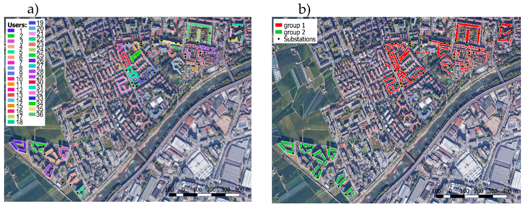
The thermal consumptions data are delivered by the smart heat meters of Bozen-Bolzano DH, which collect the average thermal power of each substation every 15 min. A total of 36 users have been selected, concerning only the complete time series of residential buildings (see
Figure 1a). In this study, a user is defined as one or more residential buildings with homogeneous characteristics fed by one or more substations connected with the DH. Two groups have been identified in
Figure 1b: users of group 1 regard non-energy-renovated blocks, which are typical of the old public housings located in the city centre, while users of group 2 are principally new generation and energy-renovated constructions placed in a new residential area.
The other time series required by the proposed method regards the outside temperature, which has been supplied by the weather station of S. Maurizio every 10 min. In order to have a dataset with a uniform time step, the outside temperature has been aggregated to 15 min.
Hence, we have checked the dataset to avoid errors due to malfunctioning of the meters, the data loggers, or the transmission system. To focus on the most challenging period for DH, we selected the heating season, which starts on 15 October 2015 and ends on 15 April 2016 [
47].
Given the heterogeneousness of the selected dataset regarding different heat demand users, it is possible to assert that the sample is significant for the thermal energy of residential users of Bozen-Bolzano during the heating season.
4. Calculation
4.1. Subsection
The selected users have been divided into two groups according to the shape of their daily thermal load pattern (
). Indeed, energy-efficient and non-energy-renovated buildings differ not only for heat consumption per meter square, but also for the operation setting of the housing heating systems.
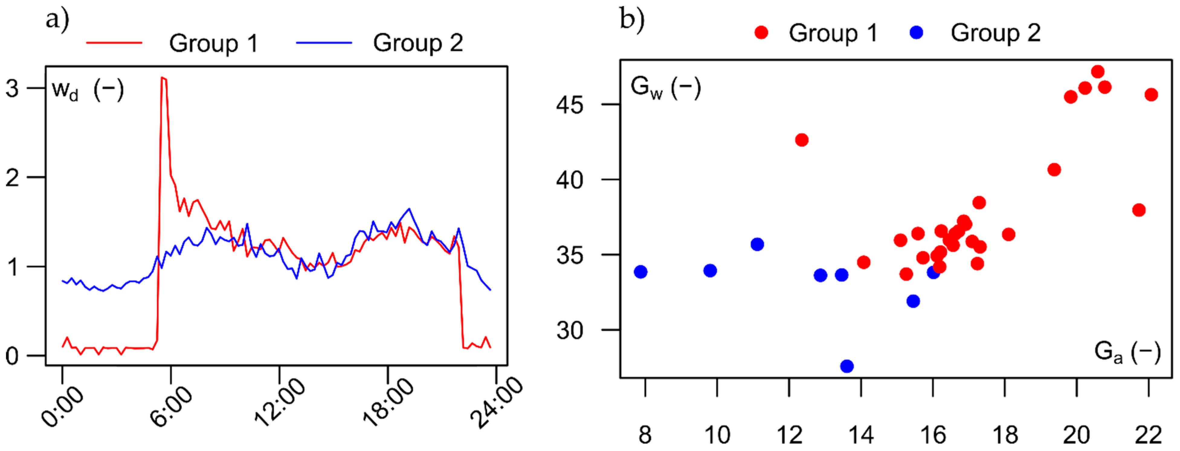
Figure 2a shows the main characteristics of each group in terms of the heat load pattern during the day.
On one side, group 1 (
Figure 2a—red line) is characterized by a night setback control which leads to a null (or very low) heat load during the night, a sharp peak between 5:00 and 6:00 a.m. (due to the reheating of the entire secondary heating system) and a final second lower spike that occurs at dinner time. This heat load behaviour is typical of the home heating systems of old/non-energy-renovated buildings which consist of high-temperature traditional radiators. The night setback control allows for saving energy.
On the other side, group 2 (
Figure 2a—blue line) is the standard heat load behaviour of the new/energy-renovated buildings featured by the home heating systems with low-temperature radiant panels. The heat load pattern presents moderate differences due to a continuous operation setting that maintain the temperature to a specific set point throughout the entire day. The morning and evening smooth peaks correspond to the increase in hot water requests (e.g., cooking, showering, etc.) and are not due to changes in space heating demand.
To assess the goodness of the user grouping, the selection has been validated by Gadd [
48] variance indexes:
, the annual relative daily variation in Equation (8), and
, the annual relative seasonal variation in Equation (9), as follows:
where
is the time discretisation interval of a day fixed to 15 min.
Figure 2b presents
versus
for the selected users, highlighting that users within the same group are located in the same area of the graph.
The intra-daily analysis, as mentioned in
Section 2, relies on the global stationary trends’ assumption of the daily heat load patterns (
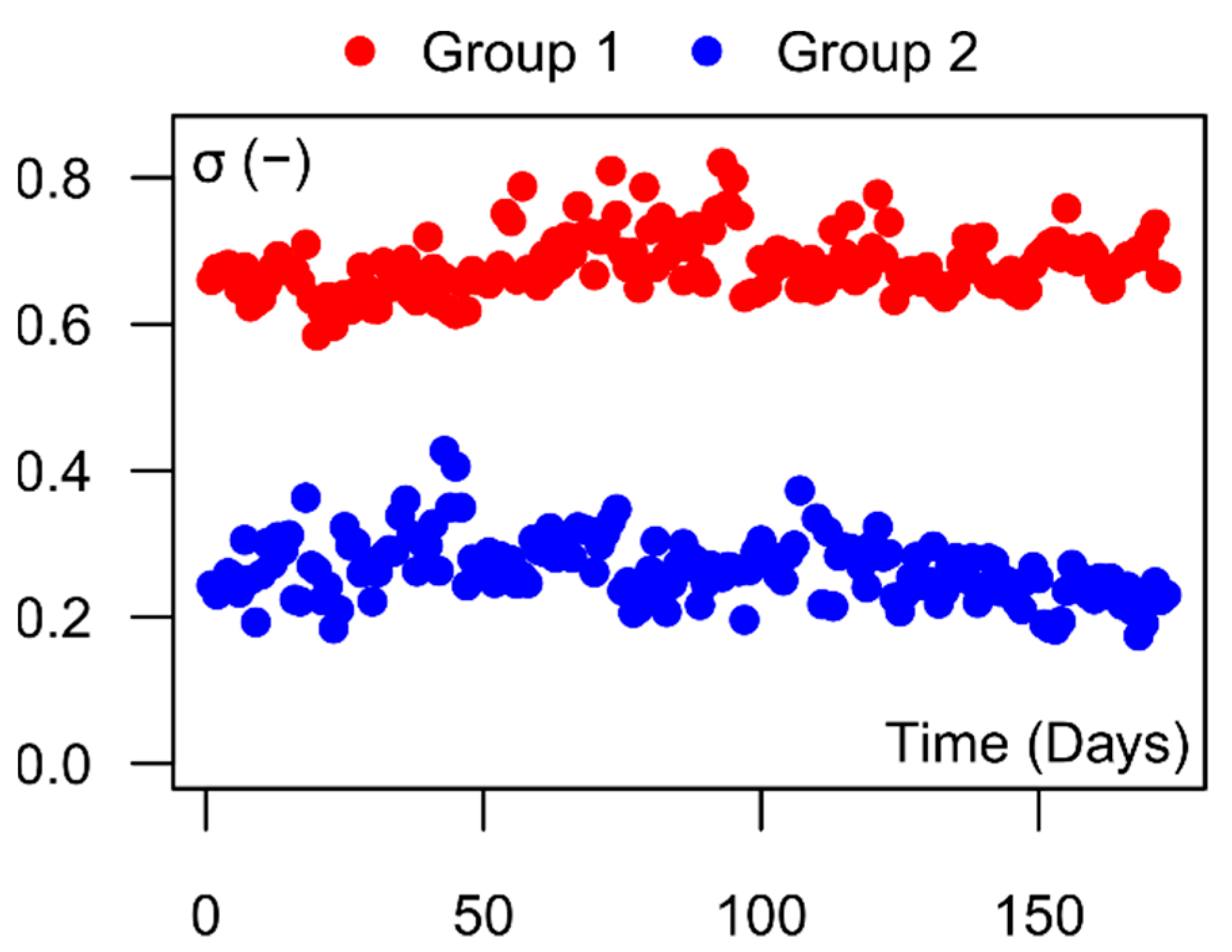
) during the heating season, that have been checked as follows. First, the time series do not present trends due to their unidimensional nature (daily mean equal to one). Second, the recursive daily seasonal component can be regarded as a stable seasonal pattern in agreement with the concept of the cyclostationary process (a process with a periodic mean and a periodic autocorrelation function). Third, the time series are also stationary in variance, which means homoscedasticity of the residuals, checked by means of daily variance plots. For instance,
Figure 3 presents the daily variance of users 4 and 23, which belong, respectively to groups 2 and 1, resulting stationary even if on different levels, due to the type of control system and the number of aggregated apartments. As shown for the two users in
Figure 3, which are different for size and energy performance, the same stationary behaviour of the daily variance is found in all other users of the analysed sample.
Indeed, the non-energy-renovated users (group 1) are characterised by a greater intra-daily variability than energy-efficient users (group 2). This propriety regarding the daily demand variation is also shown in
Figure 2a and quantified by the annual relative daily variation index
[
48] (
Figure 2b vertical axis). Finally, time series are tested through the Dickey–Fuller test for unit root [
49] rejecting the null hypothesis of non-stationarity for each time series.
4.2. Estimation of the Aggregation Relationship
With regard to the stochastic approach proposed, the two main required statistical parameters are the mean () and the coefficient of variation , which is a standardised measure of dispersion, of the daily heat load pattern () for each time interval of the day. The CV can be estimated in different ways; the first and most robust of which is through an analysis of direct measurements. This option is feasible only when such measurements are available with sufficient duration and quality. Unfortunately, in many real-life applications, direct measurements are not always available. Furthermore, it is very interesting to characterise these stochastic parameters with time series data available to the infrastructure management companies on a sample of users. For this reason, in this study, analysis of the dependence of these stochastic parameters on variables easily available to the stakeholders has been performed.
The selected non-statistical parameter considered as the main driver for the estimation of the first and second-order moments is the annual heat demand required by the considered users or group of users. This value is usually easily obtained by the managing company, as, for example, it is obtained by multiplying the energy class (
) by the heating surface (HS), as in Equation (10):
The energy class represents the energy required in one year for heating in a dwelling per unit of surface, measured in kWh/m2/year, while the heating surface is the nominal area of the dwelling. These two values are easily obtainable: the heating surface is available to municipalities for tax reasons, and the energy class is required for house energy rating. However, other, more accurate ways of deriving P are allowed in this procedure, e.g., the direct use of the yearly metered data.
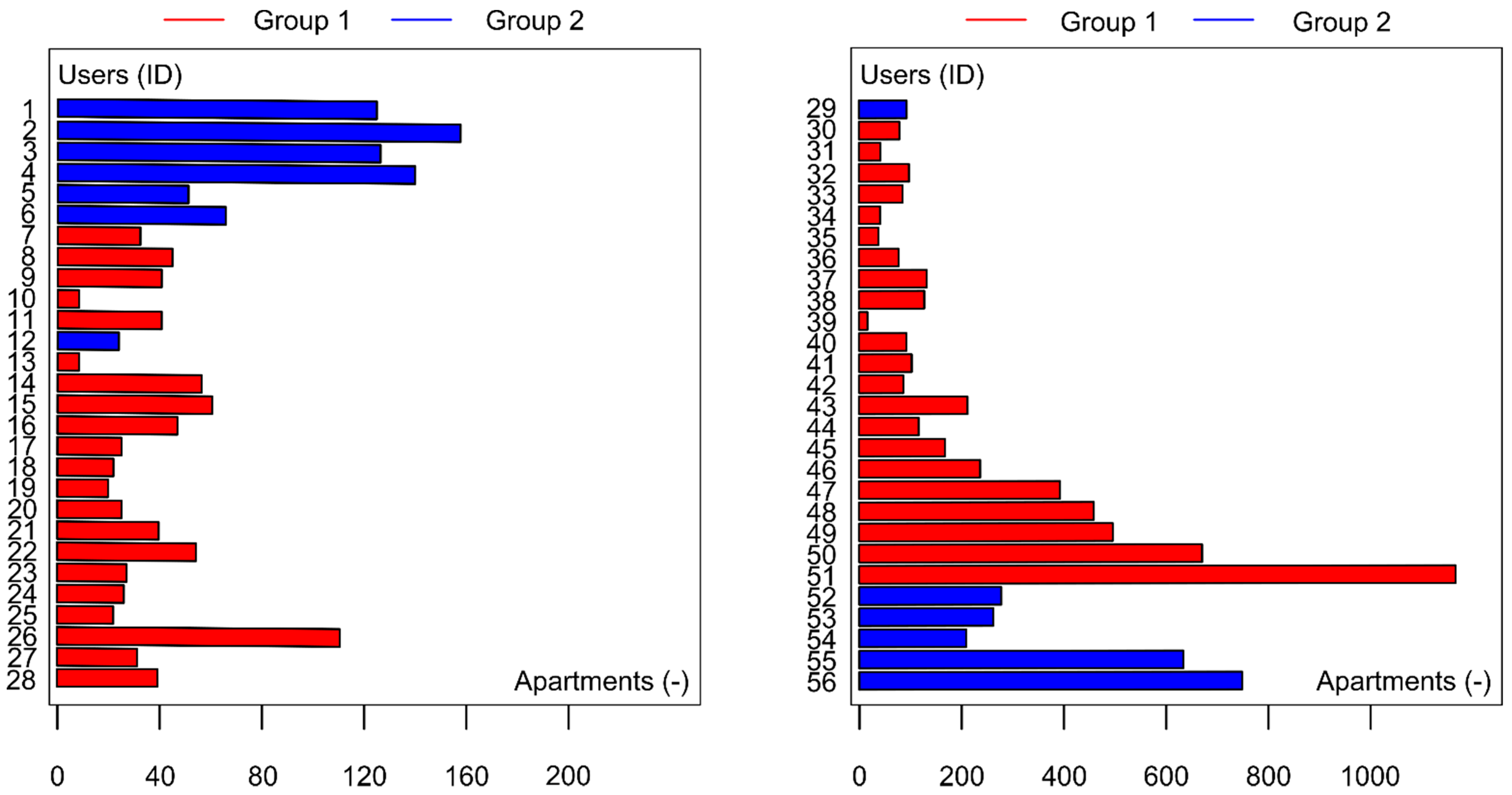
To establish a proper relationship, which has to be able to catch the effect of different users’ aggregation, the data set was enlarged with new time series of demand generated by summing the time series of real users of the same groups. Thus, the new synthetic users consist of the random aggregation of a variable number of real homogeneous users, meaning buildings with the same heat demand behaviour. In this way, the method can handle aggregation up to the district scale.
Figure 4 represents the number of apartments for each user belonging to group 1 and group 2, which consist of 28 real users and 15 aggregated users (from ID 37 to 51), and 8 real users and 5 aggregated users (from ID 52 to 56), respectively. The wide aggregation range considered, between some ten to over a thousand apartments, allows us to obtain a flexible
-
relationship for Bozen-Bolzano.
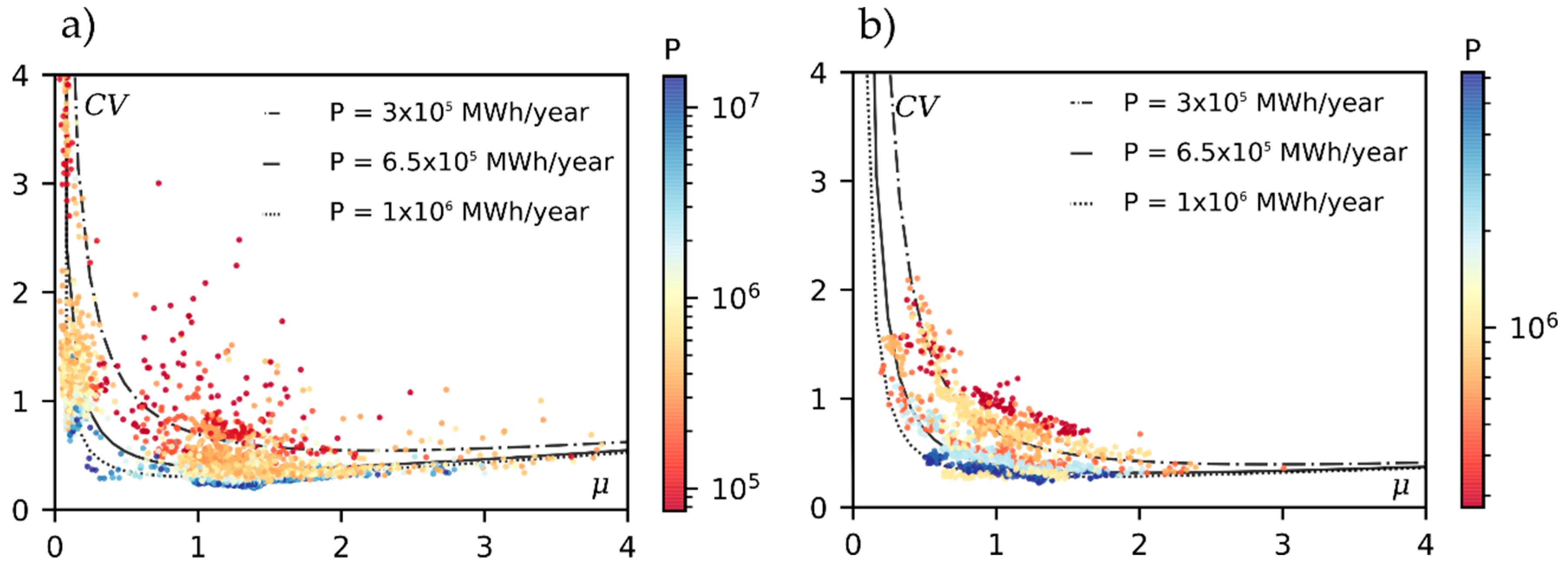
Figure 5 presents the
-
plots for group 1 and 2, respectively. The circles represent the values of the real and aggregated users coloured according to their annual heat load demand (P). It is possible to notice that, for both groups, there is an inverse proportional relationship between the first and second-order moments, e.g., [
33]. This ratio varies according to the parameter of the annual consumption; in particular, the greater this parameter P in kWh/year, the more the values are flattened on the axes, and consequently the corresponding function.
On the basis of the relationship between
and
, and the P parameter of the real data, Equation (11) has been derived. This equation displays the proposed relation through a parametric hyperbola which considers three constants to be calibrated,
,
, and
, in addition to the annual consumption P calculated using Equation (10).
The
,
, and
parameters differ for the two considered groups, and their values are reported in
Table 1. The lines in
Figure 5 show the results of Equation (11) for different values of P both for groups 1 and 2, following well the behaviour of the real data (circles) with similar aggregation parameters.
4.3. Selection of the Distribution of Daily Pattern
The available dataset has the time series of the heat load of several users with a temporal resolution of 15 min, so the day is divided into 96 intervals. Each time interval has been considered as an independent phenomenon, which consists of a sample of values regarding the monitored heating period. Thus, considering each user and aggregation of users, for each time interval, the three distributions were fitted to the observed heat load cumulated frequencies. Independent modelling of each time interval allows us to properly calculate the confidence interval of the heat demand prevision that varies throughout the day.
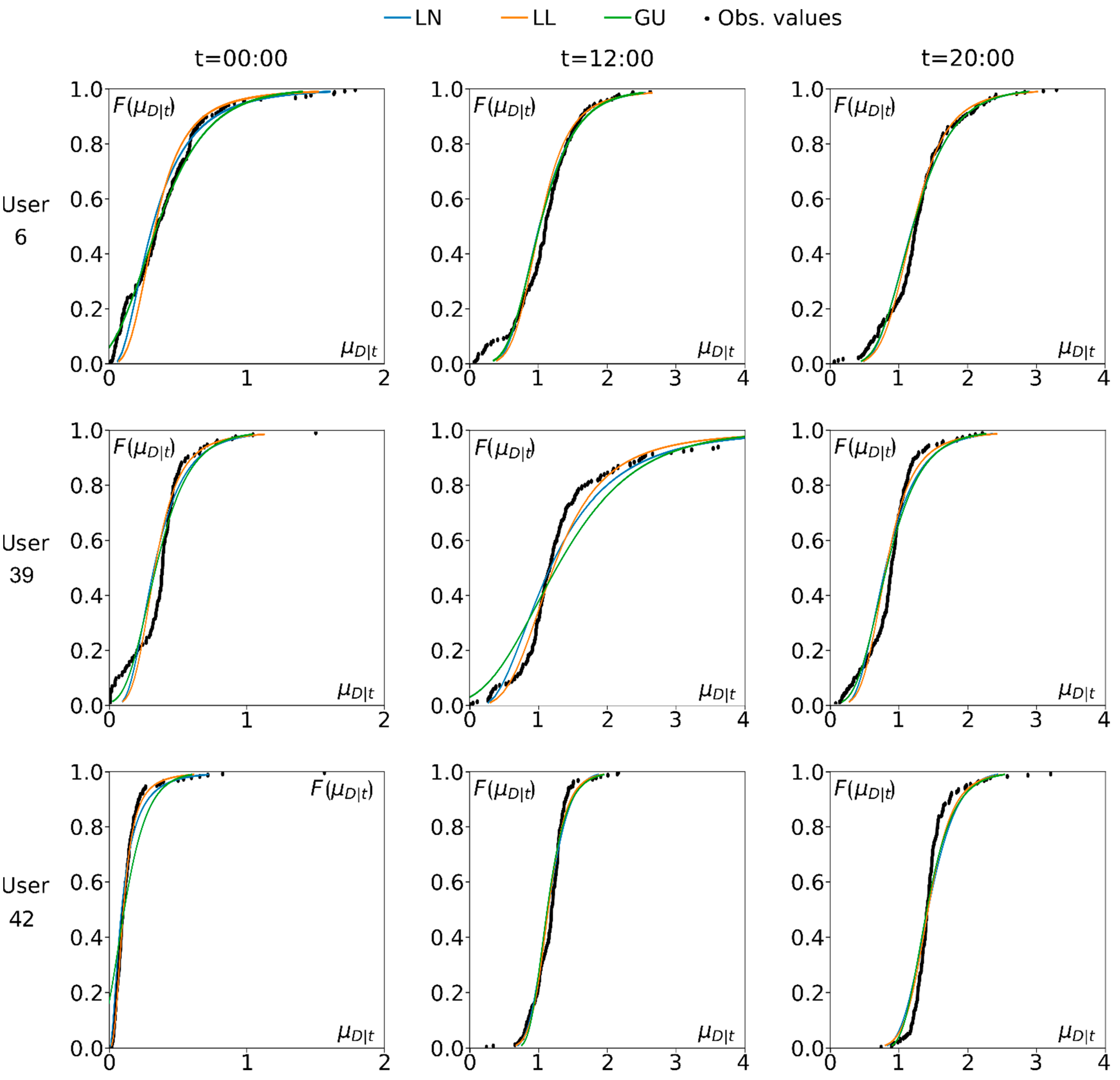
Figure 6 shows the comparison between the observed cumulated frequencies and the theoretical cumulative distribution functions Log-Normal, Log-Logistic, and Gumbel for three representative users at three different times of the day, which are interesting from an engineering point of view.
On the basis of the graphical results in
Figure 6, all three distributions fit well the observed data. However, the Gumbel distribution presents negative values at some times of the day, especially during the night (see the first column of
Figure 6 corresponding to midnight). While the Log-Logistic and Log-Normal show the best fit during the night, also avoiding negative value as probability function defined positive.
Thus, the goodness of the Log-Logistic, Log-Normal, and Gumbel is evaluated by means of the Kolmogorov-Smirnov (KS) [
50] test for all users. Indeed, KS considers the maximum drift between the observed and theoretical distribution as a goodness-of-fit measure. The KS test is applied on 96 times of the day for each of the 56 users, leading to 58% of rejection of the null hypothesis (defined as the reference pdf is equal to the empirical pdf) for Log-Logistic distribution, 62% of rejection for Log-Normal distribution, and 67% for Gumbel, with the level of significance set at 0.01. The results indicate that the Log-Logistic probability distribution has the best fit on the selected dataset.
The mediocre results obtained with the KS test are due to the use of the method of moments, which is less accurate compared to other methods such as the maximum likelihood method. However, the authors prefer the former method for this proposed procedure to be able to set the model simply with the mean and the CV of the demand, without needing a complete dataset.
4.4. Linear Regression of Seasonal Trend
After showing the differences between users of different groups on the basis of intra-daily behaviour, we have analysed the seasonal heat load pattern (
) separately. Despite the expectations, the seasonal pattern of the two groups presents the same behaviour, leading to the estimation of only one linear regression model suitable for all the analysed users.
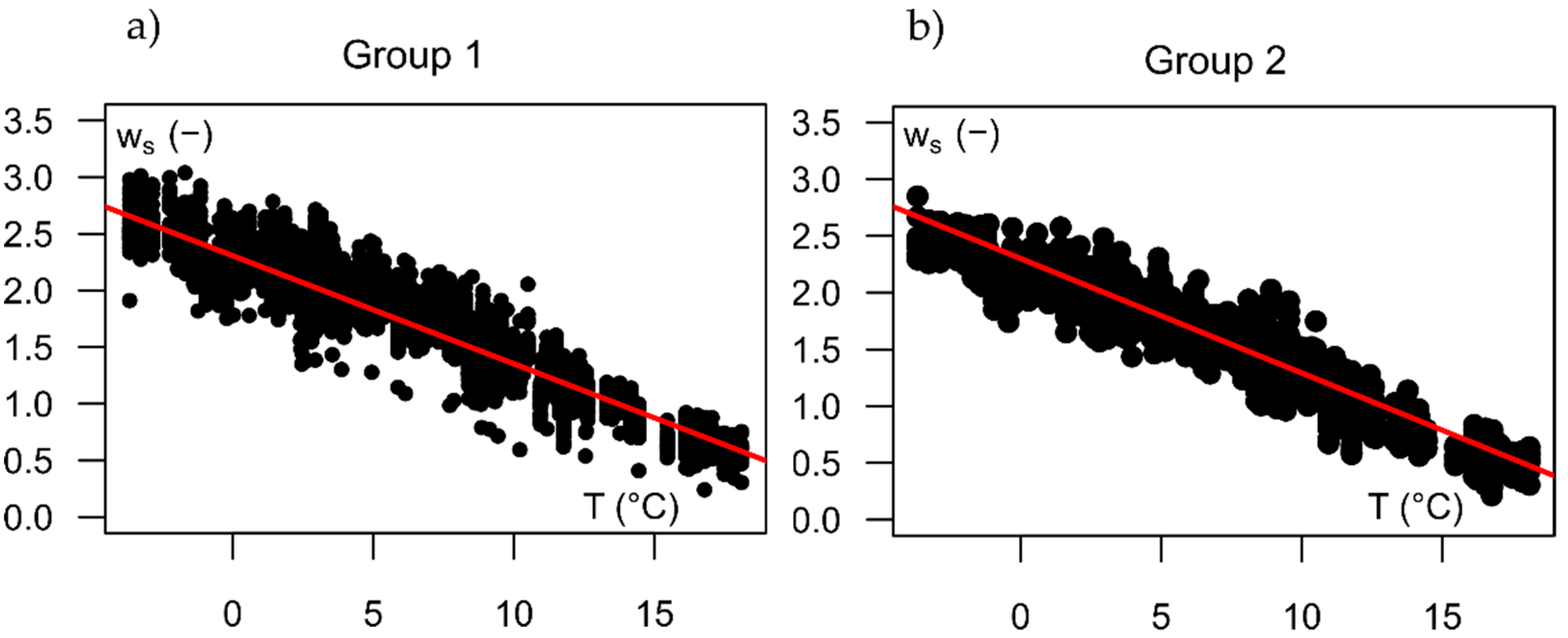
Figure 7 shows the linear behaviour of the dependence between the seasonal heat load pattern and the outdoor temperature, highlighting the similar trend of the two user groups. It means, first, that
is strongly correlated to outdoor temperature in agreement with [
51], and second, that
, which is a dimensionless variable, is independent of the buildings energy performance and the type of heating control systems. The later outcome is particularly significant as it states that the dimensionless behaviour of the daily heat demand of residential users during the heating season is uncorrelated with building proprieties. Thus, this characteristic enables the use of a unique relationship for estimating the seasonal component
defined only with the daily outside temperature for each type of users.
We have fitted the linear regression model with the least-squares method, yielding the Equation (12):
The red lines in
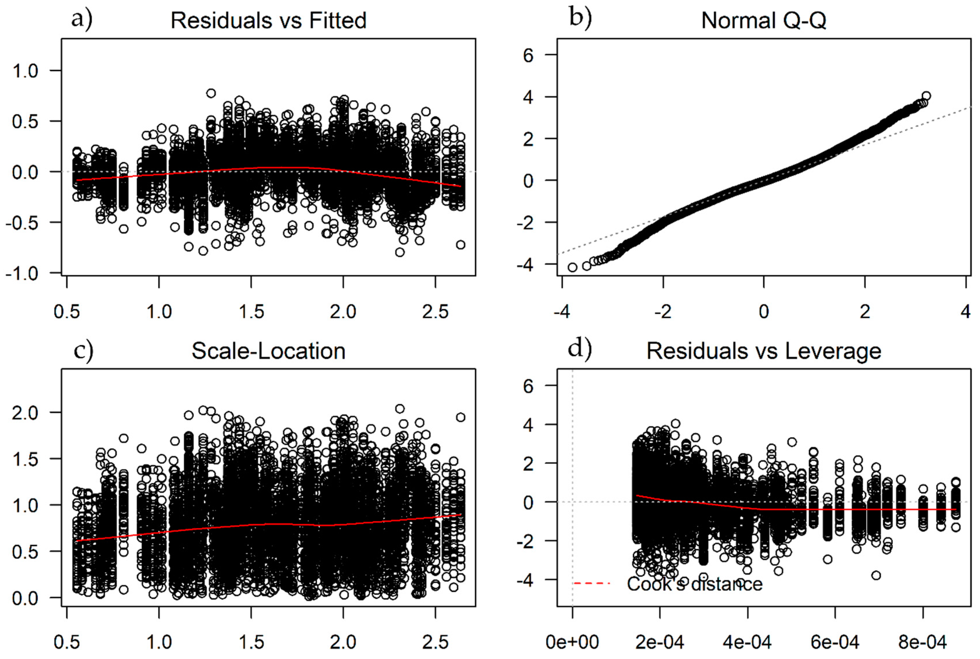
Figure 7a,b represent the estimated seasonal linear regression trend. To check the proper linear regression modelling, the assumptions of this model have been verified according to [
52]. The mean of residuals is close to zero, and the variance can be considered without any trend. The homoscedasticity of the residuals has been checked with
Figure 8a,c, which represent the residuals and standardized residuals versus the fitted values. Then, the normality of the residuals has been verified through the Q-Q plot in
Figure 8b. Finally, the absence of correlation between the residuals and the predictor variable has been tested with null Pearson’s correlation.
5. Results and Discussion
In this section, we propose an application of the estimated model (in
Section 4) for providing a three-day heat load forecasting and the corresponding confidence boundaries of two users of Bozen-Bolzano. User 51 has been selected for representing a district of group 1; it consists of about 1200 apartments (heating surface of
) with the average performance (
) of
. On the other side, user 56 represents a district belonging in group 2, which is characterised by about 750 apartments (heating surface of
) with
. These two users aim to represent the district scale of different types of buildings due to their high number of apartments aggregated.
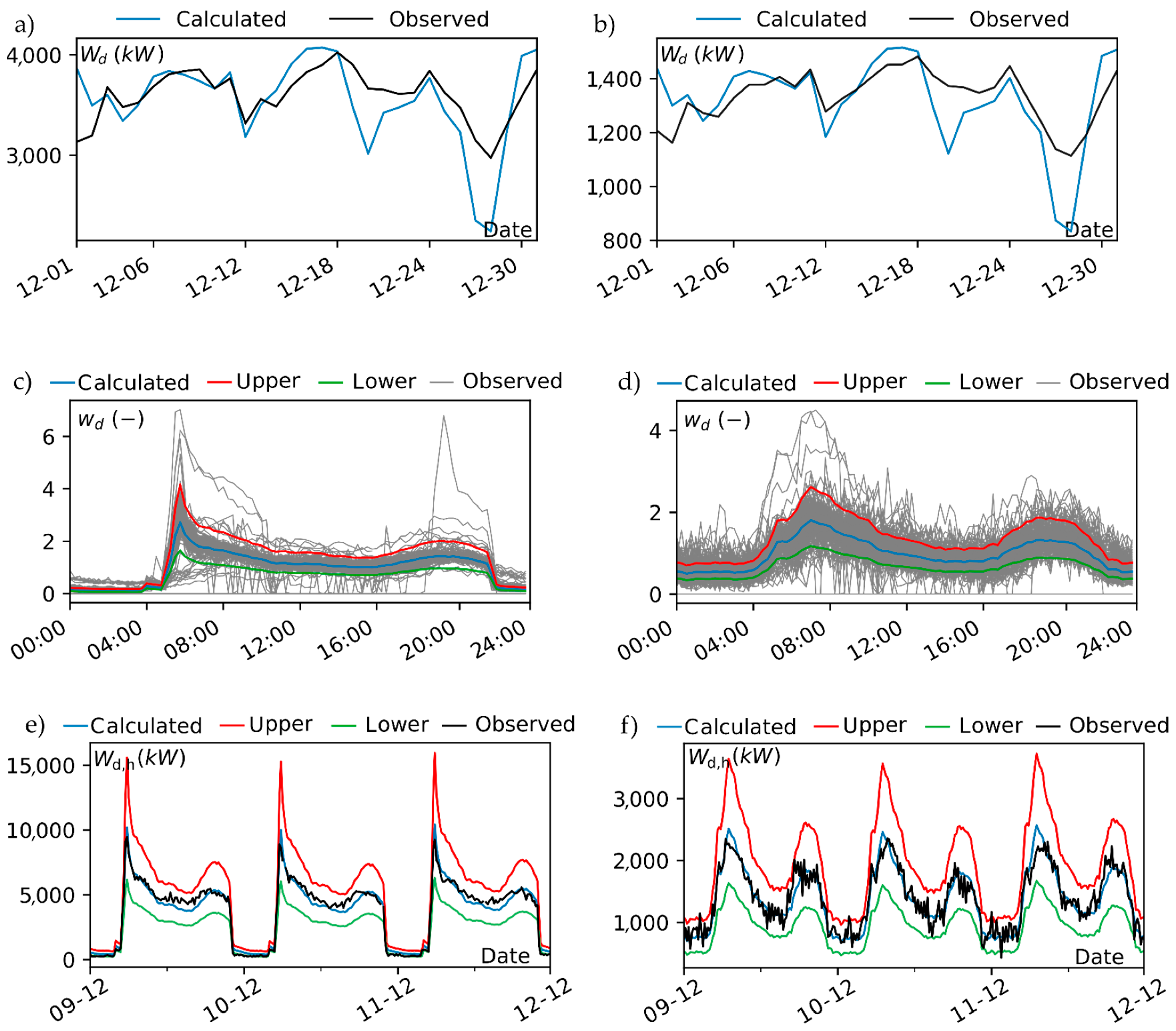
Consisting of a calculated model of seasonal and daily heat load components, and the aggregation relationship for both the defined groups, based on a sample of users’ time series, the heat load prediction has examples collecting base information about the selected district (such as the group, and the total annual heat demand (P)), and the daily temperature concerning the involved period. Thus, the forecasting has been performed over three days which range between 9 December 2016 and 11 December 2016. First, the daily average heat load has been calculated, given the outdoor temperature through the linear regression model, which is applicable to both groups, and the annual average demand (
).
Figure 9a,b presents the daily average heat load of the two districts, highlighting the similar behaviour between users of different groups.
Second, knowing the mean daily pattern of the selected users, the aggregation relationship allows us to calculate the corresponding
CV for each time of the day. Therefore, the intra-daily component has been defined through the Log-Logistic probability distribution that provides the confidence interval of the heat demand prevision.
Figure 9c,d indicates the intra-daily patterns of 2016 compared with confidence boundaries set to the 5th and 95th percentiles and the mean pattern. It is worthy to note the different behaviour between the two users due to the different heating control systems, as described in
Section 4.1.
Finally,
Figure 9e,f shows the final three-day heat load prevision merging the seasonal and intra-daily components. The heat load predicted is very close to the measured data and is entirely contained between the two boundaries in both applications. However, the measured heat load of user 56 in
Figure 9e shows unpredictable oscillation, which can be imputable mainly to the stochastic behaviour of the hot water demand.
These two previsions of heat load at the district level underline the advantages of the proposed methodology that lies in the flexibility of parameter estimation for a different users’ aggregation, the easy setting of the superimposition model on base users’ information, and the accuracy of the final results. In addition, the upper and lower boundaries give crucial information on the probability that the predicted values are included in a defined confidence interval, 5th and 95th percentiles in
Figure 9c,d, respectively. It is worth noting that good performances are achieved even for heat demand peaks, well-known times of the day in which the demand is difficult to model and predict.
6. Conclusions
We analysed the heat load behaviour of residential users connected to district heating during the heating season, adopting a data-driven approach based superimposition procedure. The final aim of the presented methodology is to provide a flexible heat demand modelling, applicable at the district level for heat load characterisation and forecasting. The analysis at the district scale has recently become a fundamental topic due to the necessity of supporting the smart energy grids, which are crucial for future sustainable energy systems. However, the well-developed methods at building and urban scale are not adaptable to the new purpose due to the excessive data needed and the poor accuracy, respectively. Therefore, this study seeks to bridge the gap in heat load forecasting at the district level through an ad hoc stochastic method.
More precisely, the proposed procedure follows a superimposition approach by characterising the seasonal and the intra-daily heat load behaviour separately. The seasonal component was modelled by studying the relationship between the daily average heat demand and the corresponding outside temperature using a linear regression model. On the other side, the daily component was analysed with bi-parametric distributions for each time of the day. The use of distribution probability functions provides information not only on the prevision, but also on the confidence intervals of the heat demand during the day.
A preliminary initial operation was necessary for investigating the different types of daily patterns presented in the dataset, and so the users were divided into homogenous groups according to their shape load pattern. The similar behaviour of the users belonging to different groups has consented to model each group separately, and thus to ensure more accurate results.
In addition, the variability of the intra-daily pattern was calculated through a proper relationship that links the coefficient of variation with the mean of the demand during the day. This formula allows to directly provide the second-order moment given the mean value and an aggregation parameter (annual heat demand), for the intra-daily component analysis.
After configuring the model with high-quality smart meter data of a sample of users, the forecasting procedure was applied on a group of monitored buildings to perform a district heat prevision over three days, but also to check the accuracy of the method on real measured consumption data. Despite this application, necessary for proving the accuracy of the model, the main advantages of the proposed methodology lie in the possibility of setting up the model on a sample of metered users, and then to perform the forecasting at the district level on the basis of a few standard details about the users of the investigated area, e.g., the type of heat control system and the annual heat demand.
The findings of this study have a doubly useful implication for supporting district heating. On one hand, the three-day previsions are crucial from an operational point of view, such as optimisation of the heat production schedule and improvement of the heat distribution management. On the other hand, the proposed procedure could be coupled with a weather model for performing long term forecasting. This type of prevision is critical for the proper planning, design, and revamping of district heating grids.
This approach may be further developed, adding a new component to the presented procedure to take into account other effects of the heat demand, such as vacation days. Additionally, an extension of the presented method may be considered regarding the non-heating season demand, which means regarding only for hot water purposes. Finally, a generalisation of the proposed methodology would be welcome by applying it to data sets collected in cities at different latitudes.
Author Contributions
Conceptualization, A.M., S.S., M.R. and R.G.; Data curation, A.M. and S.S.; Formal analysis, A.M., S.S., M.R. and R.G.; Funding acquisition, M.R.; Investigation, A.M. and S.S.; Methodology, A.M., S.S., M.R. and R.G.; Project administration, M.R.; Software, A.M. and S.S.; Supervision, M.R. and R.G.; Validation, A.M. and S.S.; Visualization, A.M. and S.S., Writing—original draft, A.M. and S.S.; and writing—review and editing, A.M., S.S., M.R. and R.G. All authors have read and agreed to the published version of the manuscript.
Funding
This work was supported by the Open Access Publishing Fund of the Free University of Bozen-Bolzano and by the internal project “TESES-Urb—Techno-economic methodologies to investigate sustainable energy scenarios at urban level” of the Free University of Bozen-Bolzano.
Data Availability Statement
Data are contained within the article.
Acknowledgments
The authors acknowledge Alperia and the Bozen-Bolzano province for providing the analysed data.
Conflicts of Interest
The authors declare no conflict of interest.
Nomenclature
| Nomenclature | Units | Definition |
| day | day of the selected period |
| (-) | total number of the day of the selected period |
| kWh//year | annual heat demand per unit of heating surface |
| (-) | annual relative daily variation index |
| (-) | annual relative seasonal variation index |
| | heating surface |
| (-) | quarter-hour time interval of a day |
| (-) | total number of the daily time step |
| kWh/year | total annual heat demand |
| °C | mean daily outdoor temperature |
| (-) | daily heat load pattern |
| (-) | seasonal heat load pattern |
| kW | thermal power demand |
| kW | annual average thermal power demand |
| kW | daily average thermal power demand |
References
- Mathiesen, B.V.; Lund, H.; Karlsson, K.B. 100% Renewable energy systems, climate mitigation and economic growth. Appl. Energy 2011, 88, 488–501. [Google Scholar] [CrossRef]
- Fankhauser, S. Valuing Climate Change: The Economics of the Greenhouse; Routledge: London, UK, 2013. [Google Scholar]
- Mazhar, A.R.; Liu, S.; Shukla, A. A state of art review on the district heating systems. Renew. Sustain. Energy Rev. 2018, 96, 420–439. [Google Scholar] [CrossRef]
- Lund, H.; Østergaard, P.A.; Chang, M.; Werner, S.; Svendsen, S.; Sorknæs, P.; Thorsen, J.E.; Hvelplund, F.; Mortensen, B.O.G.; Mathiesen, B.V.; et al. The status of 4th generation district heating: Research and results. Energy 2018, 164, 147–159. [Google Scholar] [CrossRef]
- Lund, H. Renewable Energy Systems: A Smart Energy Systems Approach to the Choice and Modeling of 100% Renewable Solutions; Academic Press: Cambridge, MA, USA, 2014. [Google Scholar]
- Rémillard, B.; Scaillet, O. Testing for equality between two copulas. J. Multivar. Anal. 2008, 100, 377–386. [Google Scholar] [CrossRef] [Green Version]
- Guelpa, E.; Toro, C.; Sciacovelli, A.; Melli, R.; Sciubba, E.; Verda, V. Optimal operation of large district heating networks through fast fluid-dynamic simulation. Energy 2016, 102, 586–595. [Google Scholar] [CrossRef]
- Righetti, M.; Bort, C.M.G.; Bottazzi, M.; Menapace, A.; Zanfei, A. Optimal Selection and Monitoring of Nodes Aimed at Supporting Leakages Identification in WDS. Water 2019, 11, 629. [Google Scholar] [CrossRef] [Green Version]
- Suganthi, L.; Samuel, A.A. Energy models for demand forecasting—A review. Renew. Sustain. Energy Rev. 2012, 16, 1223–1240. [Google Scholar]
- Wang, Z.; Srinivasan, R. A review of artificial intelligence based building energy use prediction: Contrasting the capabilities of single and ensemble prediction models. Renew. Sustain. Energy Rev. 2016, 75, 796–808. [Google Scholar] [CrossRef]
- Ma, W.; Fang, S.; Liu, G.; Zhou, R. Modeling of district load forecasting for distributed energy system. Appl. Energy 2017, 204, 181–205. [Google Scholar] [CrossRef]
- Lake, A.; Rezaie, B.; Beyerlein, S. Review of district heating and cooling systems for a sustainable future. Renew. Sustain. Energy Rev. 2017, 67, 417–425. [Google Scholar] [CrossRef]
- Sun, Q.; Li, H.; Ma, Z.; Wang, C.; Campillo, J.; Zhang, Q.; Wallin, F.; Guo, J. A Comprehensive Review of Smart Energy Meters in Intelligent Energy Networks. IEEE Internet Things J. 2015, 3, 464–479. [Google Scholar] [CrossRef]
- Uihlein, A.; Eder, P. Policy options towards an energy efficient residential building stock in the EU-27. Energy Build. 2009, 42, 791–798. [Google Scholar] [CrossRef]
- Jaggs, M.; Palmer, J. Energy performance indoor environmental quality retrofit—A European diagnosis and decision making method for building refurbishment. Energy Build. 2000, 31, 97–101. [Google Scholar] [CrossRef]
- Sailor, D.J.; Lu, L. A top–down methodology for developing diurnal and seasonal anthropogenic heating profiles for urban areas. Atmos. Environ. 2004, 38, 2737–2748. [Google Scholar] [CrossRef]
- Siwei, L.; Huang, Y.J. Energy conservation standard for space heating in Chinese urban residential buildings. Energy 1993, 18, 871–892. [Google Scholar] [CrossRef]
- Asare-Bediako, B.; Kling, W.; Ribeiro, P. Future residential load profiles: Scenario-based analysis of high penetration of heavy loads and distributed generation. Energy Build. 2014, 75, 228–238. [Google Scholar] [CrossRef]
- Pedersen, L.; Stang, J.; Ulseth, R. Load prediction method for heat and electricity demand in buildings for the purpose of planning for mixed energy distribution systems. Energy Build. 2008, 40, 1124–1134. [Google Scholar] [CrossRef]
- Ghiassi, N.; Hammerberg, K.; Taheri, M. An enhanced sampling-based approach to urban energy modelling. In Proceedings of the BS 2015—14th International IBPSA Conference, Hyderabad, India, 7–9 December 2015; pp. 626–632. [Google Scholar]
- Howard, B.; Parshall, L.; Thompson, J.; Hammer, S.; Dickinson, J.; Modi, V. Spatial distribution of urban building energy consumption by end use. Energy Build. 2011, 45, 141–151. [Google Scholar] [CrossRef]
- Newsham, G.R.; Donnelly, C.L. A model of residential energy end-use in Canada: Using conditional demand analysis to suggest policy options for community energy planners. Energy Policy 2013, 59, 133–142. [Google Scholar] [CrossRef] [Green Version]
- Sarwar, R.; Cho, H.; Cox, S.J.; Mago, P.J.; Luck, R. Field validation study of a time and temperature indexed autoregressive with exogenous (ARX) model for building thermal load prediction. Energy 2017, 119, 483–496. [Google Scholar] [CrossRef]
- Powell, K.M.; Sriprasad, A.; Cole, W.J.; Edgar, T.F. Heating, cooling, and electrical load forecasting for a large-scale district energy system. Energy 2014, 74, 877–885. [Google Scholar] [CrossRef]
- Gu, W.; Wang, Z.; Wu, Z.; Luo, Z.; Tang, Y.; Wang, J. An Online Optimal Dispatch Schedule for CCHP Microgrids Based on Model Predictive Control. IEEE Trans. Smart Grid 2016, 8, 2332–2342. [Google Scholar] [CrossRef]
- Tsai, C.-L.; Chen, W.T.; Chang, C.-S. Polynomial-Fourier series model for analyzing and predicting electricity consumption in buildings. Energy Build. 2016, 127, 301–312. [Google Scholar] [CrossRef]
- Kuo, P.-H.; Huang, C.-J. A High Precision Artificial Neural Networks Model for Short-Term Energy Load Forecasting. Energies 2018, 11, 213. [Google Scholar] [CrossRef] [Green Version]
- Protić, M.; Shamshirband, S.; Petković, D.; Abbasi, A.; Mat Kiah, M.L.; Unar, J.A.; Živković, L.; Raos, M. Forecasting of consumers heat load in district heating systems using the support vector machine with a discrete wavelet transform algorithm. Energy 2015, 87, 343–351. [Google Scholar] [CrossRef]
- Xue, G.; Pan, Y.; Lin, T.; Song, J.; Qi, C.; Wang, Z. District Heating Load Prediction Algorithm Based on Feature Fusion LSTM Model. Energies 2019, 12, 2122. [Google Scholar] [CrossRef] [Green Version]
- Labidi, M.; Eynard, J.; Faugeroux, O.; Grieu, S. A new strategy based on power demand forecasting to the management of multi-energy district boilers equipped with hot water tanks. Appl. Therm. Eng. 2017, 113, 1366–1380. [Google Scholar] [CrossRef]
- Reinhart, C.F.; Davila, C.C. Urban building energy modeling—A review of a nascent field. Build. Environ. 2016, 97, 196–202. [Google Scholar] [CrossRef] [Green Version]
- Menapace, A.; Righetti, M.; Santopietro, S.; Gargano, R.; Dalvit, G. Stochastic characterisation of the district heating load pattern of residential buildings. Euroheat Power 2019, 16, 14–19. [Google Scholar]
- Gargano, R.; Tricarico, C.; DEL Giudice, G.; Granata, F. A stochastic model for daily residential water demand. Water Supply 2016, 16, 1753–1767. [Google Scholar] [CrossRef] [Green Version]
- Catalina, T.; Virgone, J.; Blanco, E. Development and validation of regression models to predict monthly heating demand for residential buildings. Energy Build. 2008, 40, 1825–1832. [Google Scholar] [CrossRef]
- Wojdyga, K. An influence of weather conditions on heat demand in district heating systems. Energy Build. 2008, 40, 2009–2014. [Google Scholar] [CrossRef]
- Pacheco-Torres, R.; Ordóñez, J.; Martínez, G. Energy efficient design of building: A review. Renew. Sustain. Energy Rev. 2012, 16, 3559–3573. [Google Scholar] [CrossRef]
- Popescu, D.; Ungureanu, F.; Hernández-Guerrero, A. Simulation models for the analysis of space heat consumption of buildings. Energy 2009, 34, 1447–1453. [Google Scholar] [CrossRef]
- Amjady, N. Short-term hourly load forecasting using time-series modeling with peak load estimation capability. IEEE Trans. Power Syst. 2001, 16, 798–805. [Google Scholar] [CrossRef]
- Di Lascio, F.M.L.; Menapace, A.; Righetti, M.; Maurizio, R. Joint and conditional dependence modelling of peak district heating demand and outdoor temperature: A copula-based approach. J. Ital. Stat. Soc. 2019, 29, 373–395. [Google Scholar] [CrossRef]
- Di Lascio, F.M.L.; Menapace, A.; Righetti, M. Analysing the relationship between district heating demand and weather conditions through conditional mixture copula. Environ. Ecol. Stat. 2021, 28, 53–72. [Google Scholar] [CrossRef]
- Wu, L.; Kaiser, G.; Solomon, D.; Winter, R.; Boulanger, A.; Anderson, R. Improving efficiency and reliability of building systems using machine learning and automated online evaluation. In Proceedings of the 2012 IEEE Long Island Systems, Applications and Technology Conference, Farmingdale, NY, USA, 4 May 2012; pp. 1–6. [Google Scholar] [CrossRef] [Green Version]
- Kottegoda, N.T.; Rosso, R. Applied Statistics for Civil and Environmental Engineers; Blackwell: Malden, MA, USA, 2008. [Google Scholar]
- Gumbel, E.J. The Return Period of Flood Flows. Ann. Math. Stat. 1941, 12, 163–190. [Google Scholar] [CrossRef]
- Pal, R.; Pani, P. Seasonality, barrage (Farakka) regulated hydrology and flood scenarios of the Ganga River: A study based on MNDWI and simple Gumbel model. Model. Earth Syst. Environ. 2016, 2, 1–11. [Google Scholar] [CrossRef] [Green Version]
- Tricarico, C.; De Marinis, G.; Gargano, R.; Leopardi, A. Peak residential water demand. Proc. Inst. Civ. Eng. Water Manag. 2007, 160, 115–121. [Google Scholar] [CrossRef] [Green Version]
- Gargano, R.; Tricarico, C.; Granata, F.; Santopietro, S.; De Marinis, G. Probabilistic Models for the Peak Residential Water Demand. Water 2017, 9, 417. [Google Scholar] [CrossRef] [Green Version]
- DPR Decreto del Presidente della Repubblica n 74 (16 Aprile 2013) Regolamento Recante Definizione dei Criteri Generali in Materia Desercizio, Conduzione, Controllo, Manutenzione e Ispezione degli Impianti Termici per la Climatizzazione Invernale ed Estiva degli Edifici e per la Preparazione dell’acqua Calda per usi Igienici Sanitari, a Norma dell’articolo 4, Comma 1, Lettere a) e c), del d.lgs. 19 Agosto 2005, n.192 della Repubblica n. 74. Available online: http://www.energia.provincia.tn.it/binary/pat_agenzia_energia/dpr%2074-2013.pdf (accessed on 27 August 2021).
- Gadd, H.; Werner, S. Daily heat load variations in Swedish district heating systems. Appl. Energy 2013, 106, 47–55. [Google Scholar] [CrossRef] [Green Version]
- Phillips, P.C.B.; Perron, P. Testing for a unit root in time series regression. Biometrika 1988, 75, 335–346. [Google Scholar] [CrossRef]
- Massey, F.J., Jr. The Kolmogorov-Smirnov test for goodness of fit. J. Am. Stat. Assoc. 1951, 46, 68–78. [Google Scholar] [CrossRef]
- Goia, A.; May, C.; Fusai, G. Functional clustering and linear regression for peak load forecasting. Int. J. Forecast. 2010, 26, 700–711. [Google Scholar] [CrossRef]
- Seber, G.A.F.; Lee, A.J. Linear regression analysis; John Wiley & Sons: Hoboken, NJ, USA, 2012; Volume 329. [Google Scholar]
Figure 1.
Map of the selected sample of residential users fed by the DH of Bozen-Bolzano in (a), and map of the load-based user groups in (b).
Figure 1.
Map of the selected sample of residential users fed by the DH of Bozen-Bolzano in (a), and map of the load-based user groups in (b).
Figure 2.
Map of the selected sample of residential users fed by the DH of Bozen-Bolzano in (a), and map of the load-based user groups in (b).
Figure 2.
Map of the selected sample of residential users fed by the DH of Bozen-Bolzano in (a), and map of the load-based user groups in (b).
Figure 3.
The daily standard deviation of the daily heat load pattern on the y-axis and the days of the heating season on the x-axis of user 4 belonging to group 2 and user 23 belonging to group 1.
Figure 3.
The daily standard deviation of the daily heat load pattern on the y-axis and the days of the heating season on the x-axis of user 4 belonging to group 2 and user 23 belonging to group 1.
Figure 4.
Bar chart of the number of apartments aggregated for each user.
Figure 4.
Bar chart of the number of apartments aggregated for each user.
Figure 5.
- relationship of the daily heat load pattern () with parameter P for the two considered groups ((a) group 1, (b) group 2); the dots show the real data values and their colour the corresponding parameter P (colormap), while the lines indicate the results of Equation (11) with the parameters P as indicated in the legend.
Figure 6.
Comparison between the three cumulative distribution functions Log-Normal (LN), Log-Logistic (LL), and Gumbel (GU), and the observed cumulated frequencies of the daily heat load pattern
(-) of three users at different times of the day.
Figure 6.
Comparison between the three cumulative distribution functions Log-Normal (LN), Log-Logistic (LL), and Gumbel (GU), and the observed cumulated frequencies of the daily heat load pattern
(-) of three users at different times of the day.
Figure 7.
Seasonal heat load pattern during the period of the heating season versus outside temperature (°C) and linear regression trend (red line); group 1 in (a), and group 2 in (b).
Figure 7.
Seasonal heat load pattern during the period of the heating season versus outside temperature (°C) and linear regression trend (red line); group 1 in (a), and group 2 in (b).
Figure 8.
Graphs about residuals analysis: (a) residuals versus fitted values, (b) QQ-plot, (c) standardised residuals versus fitted values, and (d) residuals versus average.
Figure 8.
Graphs about residuals analysis: (a) residuals versus fitted values, (b) QQ-plot, (c) standardised residuals versus fitted values, and (d) residuals versus average.
Figure 9.
District heat load forecasting of users 51 and 56 belonging to group 1 and 2, respectively. (a,c,e) concerns user 51, while (b,d,f) user 56. (a,b) show the plot of the seasonal component, (c,d) indicate the intra-daily patterns of the heating season with the mean and boundaries (5th and 95th percentiles, respectively), and (e,f) describe the final heat load prediction of three days.
Table 1.
The , , and parameters for Equation (11).
Table 1.
The , , and parameters for Equation (11).
| | a | b | c |
|---|
| Group 1 | 1 | 0.1 | 0.1 |
| Group 2 | 1.5 | 0.05 | 0.15 |
| Publisher’s Note: MDPI stays neutral with regard to jurisdictional claims in published maps and institutional affiliations. |
© 2021 by the authors. Licensee MDPI, Basel, Switzerland. This article is an open access article distributed under the terms and conditions of the Creative Commons Attribution (CC BY) license (https://creativecommons.org/licenses/by/4.0/).


