New Infeed Correction Methods for Distance Protection in Distribution Systems

Abstract

The reliability and security of power systems may be jeopardized by the increase in the amounts of renewable generation and the uncertainties produced by these devices. In particular, the protection schemes of traditional power systems have been challenged by the integration of distributed generation (DG) resources. Distance relays (DRs), which have been mainly employed to protect transmission systems, are increasingly proposed as one of the solutions to protect distribution systems with a heavy penetration of DGs. However, conventional distance protection faces several drawbacks that might lead to maloperation. One of those challenges is the “infeed effect”, which causes the impedance seen by the distance relay to be larger than the actual positive-sequence line impedance between the fault and relay location. This paper proposes three new methods to estimate the distance to the fault in the presence of infeeds, whether in a radial distribution feeder or the transmission line. Unlike other solution methodologies in the literature that require communication links to estimate the distance to the fault, the proposed methods only need the local measurement (i.e., the voltage and current measurements at the location of the distance relay) to do the same. The performance of the method is demonstrated with a radial distribution system model in PSCAD™/EMTDC™.

1. Introduction

As opposed to traditional distribution systems (DS) in which the substation is the primary source of generation, the integration of distributed generation (DG) brings generation closer to consumers by siting generation along the feeder. DG is typically considered to be one of the following energy sources: photovoltaics (PV), small wind turbines, diesel generators, batteries, hydroelectric generators, or micro-turbines [1]. Siting small to medium power generating stations closer to the customer reduces overall energy consumption by decreasing active power losses incurred during the transmission of electricity, thereby reducing reliance on fossil fuels and improving environmental concerns. In addition, the deployment of more efficient DG-based systems reduces economic costs and aids in the development of renewable energy. In addition, integration of DG-based sources improves the operational reliability in the load centers that are remotely connected to the primary power grid and overloaded urban zones. While there are many advantages to integrating DG into the DS, the presence of DGs may complicate the existing protection of DSs, which are usually protected with overcurrent protection equipment such as overcurrent relays (OCRs) and/or fuses [2].

With the predominant integration of DGs, the traditional radial and unidirectional single-source-based distribution system configuration is changed into the bidirectional, multi-source-based distribution system [3]. Examples of the influences of DG on current protection are shown in Figure 1. At the inception of the fault, as shown in Figure 1a, the distribution substation and the DG jointly provide the fault current to the fault point. The DG fault current contribution increases the fault current. In Figure 1a, the CB1 should isolate the fault and CB2 must not operate. However, the high fault current may cause maloperation of both breakers (i.e., CB1 and CB2). The maloperation of CB2 will cause a power outage to all customers connected to the healthy feeder (i.e., the feeder with no fault). If a fault occurs downstream of the DG, as shown in Figure 1b, the fault current consists of the fault current contribution from the DG and the fault current from the distribution substation. Thus, the DG in Figure 1b decreases the fault current through CB2 compared to the case with no DG. This situation could cause a “fail-to-trip” of CB2 because the overcurrent protection sees a lower fault current than its trip settings.

The integration of DG on a distribution feeder, as shown in Figure 1c, will affect the coordination between the recloser and fuse. If a fault occurs, the fault current passing through the recloser would be lower than the fault current if there were no DG in the system. At the same time, the current through the fuse consists of the currents from the distribution substation as well as the current from the DG, which means that the fuse current is no longer the same as the current passing through the recloser. As a result, recloser–fuse coordination may be lost. Therefore, the protection philosophy of distribution systems must be reviewed and developed to overcome the new challenges posed by the integration of DG. Protection challenges due to such situations and corresponding solutions are discussed in [4,5,6]. One of the solutions that provides a reliable and secure protection scheme for DG-integrated DS is using distance relays (DR) in place of overcurrent relays [7].

DRs, which were used mainly to protect transmission systems in the past, have been proposed as one of the potential solutions to protect radial distribution systems [8,9]. The significant advantages of DR include its innate ability to detect faults in both directions (depending on the characteristics of the DR) and free from external system factors. These features make DR a favorable choice for distribution system protection in comparison to overcurrent protection [7]. However, integrating DGs in radial distribution systems may create issues that affect the reliability and sensitivity of DRs. Some of these issues include the proper setting of the zero-sequence compensation factor $K_0$, the fault resistance, and the infeed effect [10,11].

The infeed effect due to the integration of DGs in radial distribution systems causes the impedance seen by the relay to be larger than the actual positive-sequence impedance between the relay location and the fault position, causing the relay to underreach [12]. Changing the DR setting to protect a line in a distribution system equipped with one or more DGs often results in large settings. In other words, to address the infeed effect, the DR impedance settings would be increased. However, these large settings may cause maloperation of the DR during system disturbances, especially in heavy-load periods or during stable swing oscillations [12].

Some of the solutions that have been used in transmission lines to solve this problem are intertripping schemes, such as underreach with direct tripping, permissive underreach intertripping, and permissive overreach intertripping (pp. 210–213, [13]). These communication-based schemes have been proved to be a very reliable solution. Another communication-based solution, as proposed in [14], uses the real-time measurements of the current at various locations to compensate for the impedance calculated by the DR. Adjusting DR settings by using an adaptive protection scheme is proposed in [15]. The scheme relies on using remote terminal units (RTUs) to exchange data via communication links (fiber optic) between the local and remote ends of the protected line. Similarly, an adaptive distance relay setting is proposed in [16,17]. Mishra et al. [16] proposed an adaptive distance protection that modifies DR trip boundary setting based on prefault conditions of the solar photovoltaic (PV) plant (i.e., positive and negative impedances). An adaptive approach is proposed in [17] to overcome the maloperation of the distance relay in presence of infeed from static var compensator (SVC). Synchronized phasors measurement (SPM) and communication links are required for the proposed approach in [17]. In order to avoid the need for adaptive protection techniques, Tsimtsios et al. [18] proposed a pilot-based distance protection scheme. The proposed scheme is applied to meshed DS with high penetration of DGs. However, the aforementioned schemes have the disadvantage that they explicitly rely on a communication network; therefore, if the communication system fails (by either natural or cyber interference), the result will be miscoordination of the protection system. Moreover, comparing currents at line ends is expensive as it requires communication circuits to be at least as long as the lines themselves to be protected. Furthermore, the maintenance cost of these communication systems can be significant [19]. In the remainder of this paper, we propose several methods that avoid the disadvantages posed by the communication requirement.

The objective of this paper is to introduce an accurate and inexpensive approach to mitigate the infeed effect. The proposed approach is a cost-effective solution since it only requires the measurements at the relay location to estimate the distance from the DR location to the fault location in the presence of one or more distributed power sources. Hence, there is no need to install any additional hardware beyond the existing conventional protection, switching, and sensing devices.

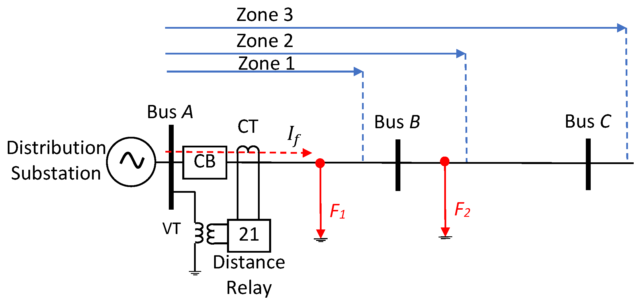
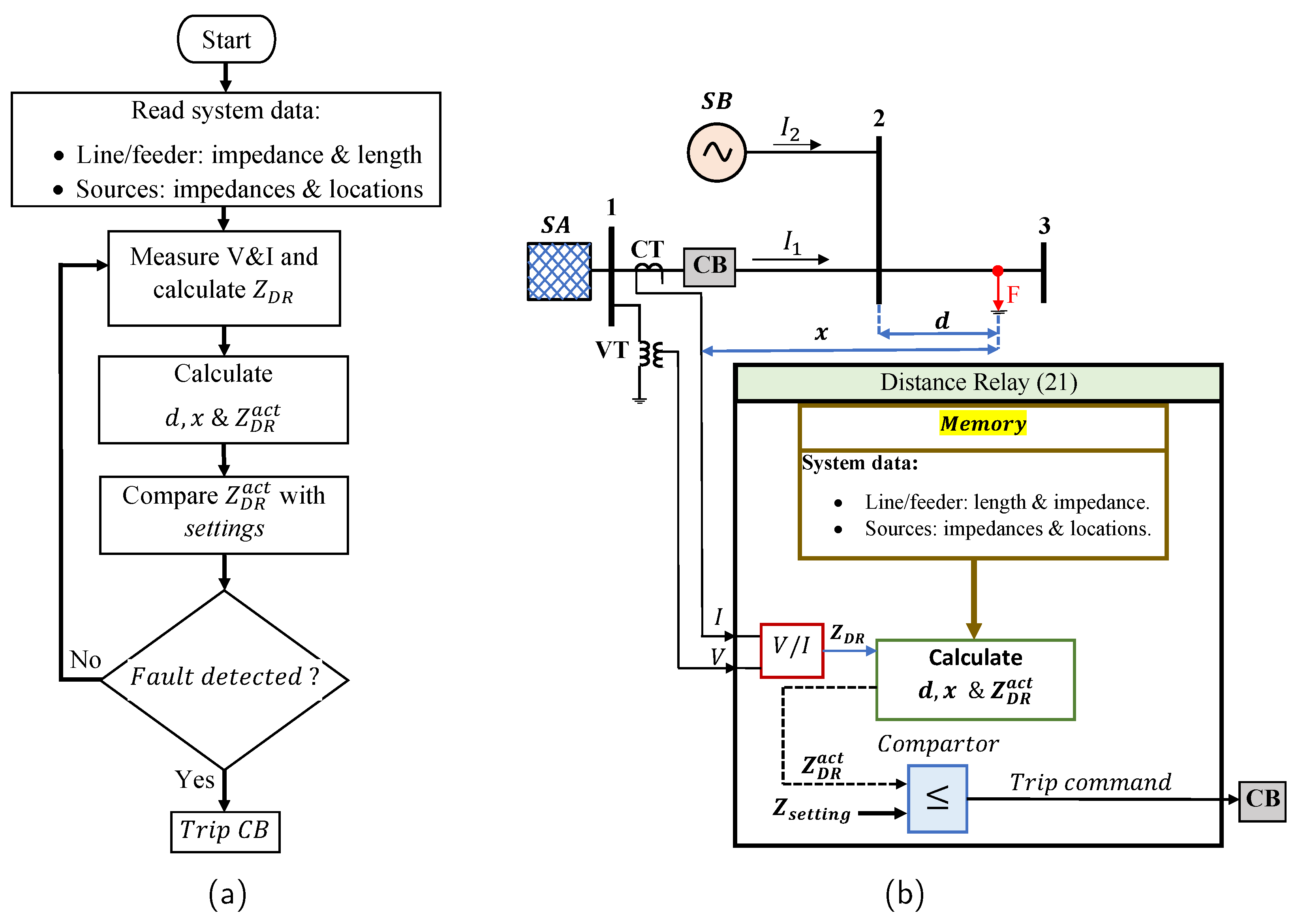
2. Distance Protection

Distance protection is based on estimating the line impedance by comparing the fault current passing through the relay against the voltage at the relay point. The feeder length protected by the distance relay is usually divided into three zones or more. Each zone covers a percentage of the line length. For example, Zone 1 usually covers about 85% of the line length from Bus A to Bus B. Zone 2 covers the entire length of the line connecting Bus A and Bus B plus a portion of the next line length (p. 184, [13]), and so on for the remaining zones, as shown in Figure 2.

The distance relay located at Bus A measures the voltage (V) and current (I) at the basic frequency, via voltage transformer (VT) and current transformer (CT), respectively. The impedance seen by the relay is:

$$Z_R=\frac{V_R}{I_R}$$

(1)

$$V_R=I_R·\alpha ·Z_{line}$$

(2)

where $V_R$ and $I_R$ are the voltage and current values measured by the relay, $\alpha$ represents the distance between the relay point and the fault point, and $Z_{line}$ is the impedance of the protected line. The value of the impedance, $Z_R$, for a fault at $F_1$ is

$$Z_R=\alpha ·Z_{lineAB}$$

(3)

and for a fault at $F_2$ is

$$Z_R=Z_{lineAB}+\alpha ·Z_{lineBC}$$

(4)

The distance relay operates when the impedance measured by the relay is less than the relay setting value. In other words, the DR will operate if the measured impedance, also known as the apparent impedance, is within its operating characteristic. This characteristic is shown most conveniently in an impedance R–X diagram, where the x-axis represents the resistance R and the y-axis represents the reactance X. There are many different DR characteristics such as mho, impedance, and quadrilateral characteristic. Choosing from these characteristics depends on many factors such as relay design, application, etc. [20]. Typical DR characteristics on a R–X diagram are shown in Figure 3.

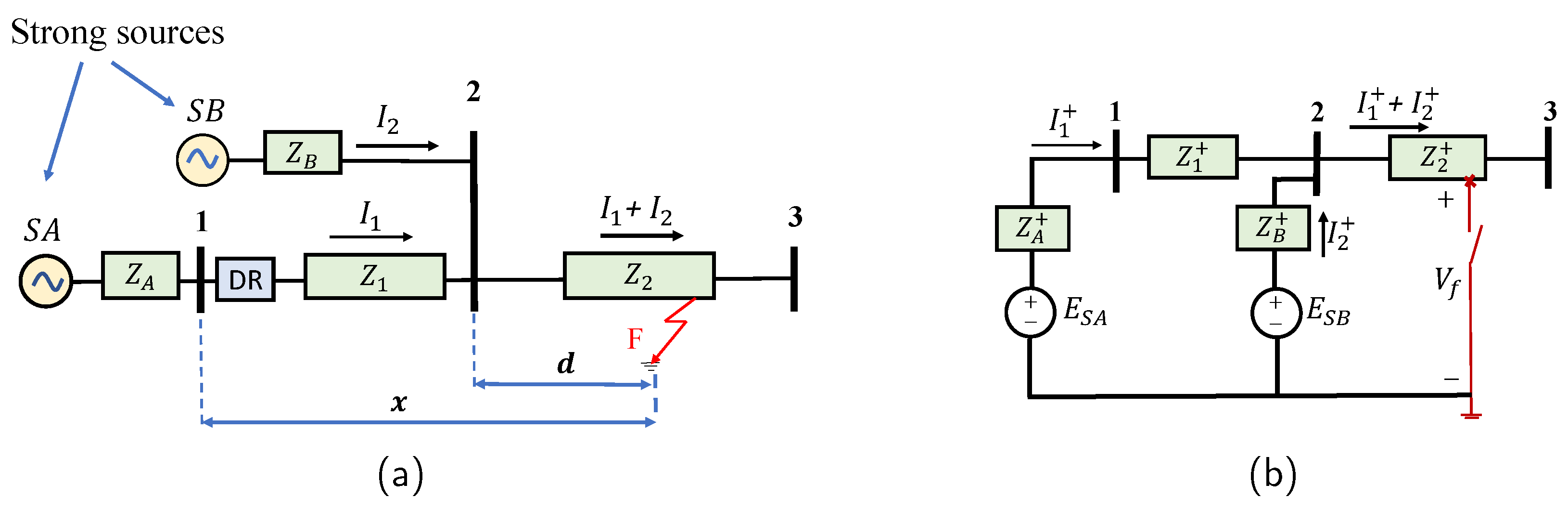
3. Infeed Effect

The infeed effect causes the impedance seen by the relay to appear to be larger than the actual positive-sequence impedance between the relay and the fault point, causing the relay to underreach. The infeed effects during non-single-line-to-ground (SLG) faults in different configurations are described in more detail in Section 3.1 and Section 3.2. Each system configuration has a particular infeed effect on the distance relay. For each system, $Z_A$, $Z_B$, and $Z_C$ are the line positive-sequence impedances. $I_S$, $I_1$, $I_2,\dots$, $I_n$ are the currents fed by the sources ${DG}_1$, ${DG}_2,\dots ,$ ${DG}_n$. A DR is utilized to protect the feeder in each configuration. The infeed effect on a ground distance relay is described in Section 3.3.

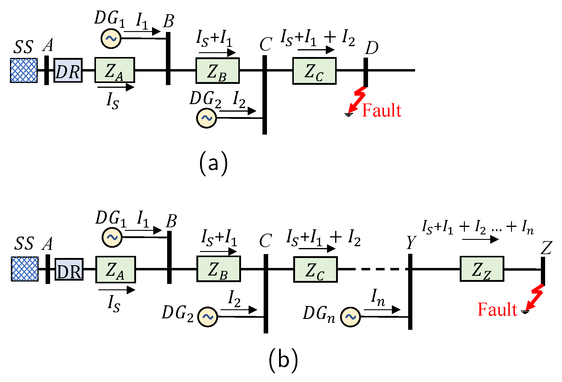
3.1. Configuration 1

A radial distribution feeder with a generation source at Bus B is shown in Figure 4a. In the case of a three-phase fault at Bus C, the measured voltage by the DR at Bus A is [13]

$$V_A=I_S{Z}_A+(I_S+I_1)Z_B$$

(5)

The positive-sequence impedance up to the fault location measured by the DR is

$$\begin{array}{ccc}\hfill Z_{DR}& =& Z_A+(1+\frac{I_1}{I_S})Z_B\hfill \\ & =& Z_A+Z_B+K·Z_B\hfill \end{array}$$

(6)

where K is defined as the infeed constant ($K=\frac{I_1}{I_S}$). Based on Equation (6), the DR at Bus A measures an impedance larger than the actual impedance between Bus A and the fault point. The additional impedance, $K{Z}_B$, impacts the DR operation and the makes DR underreach.

In Figure 4b, more than one DG are connected to the same bus. Their impact on DR measurements is

$$V_A=I_S{Z}_A+(I_S+I_1+I_2+\dots +I_n)Z_B$$

(7)

The positive-sequence impedance of the line up to the fault point, measured by the DR, is

$$\begin{array}{ccc}\hfill Z_{DR}& =& Z_A+(1+\frac{I_1+I_2+\dots +I_n}{I_S})Z_B\hfill \\ & =& Z_A+Z_B+K_n·Z_B\hfill \end{array}$$

(8)

where $K_n$ is the infeed constant ($\frac{I_1+I_2+\dots +I_n}{I_S}=\frac{{\sum }_{i=1}^n{I}_i}{I_1}$) and n is the number of DGs connected to Bus B.

The impedance–distance relation in the presence of infeeds is discussed in (pp. 186–189, [13]). The line impedance for the system in Figure 5a is shown in Figure 5b as a function of the distance. It is clear that the infeed effect changes the impedance measured by the DR at Bus A. The impedance measured by the DR in Figure 5a for two different configurations is visualized in Figure 5b. If there are no DGs in the system, the impedance measured by the DR is equal to the actual impedance of the line, which is proportional to the slope of line segment $A^{\prime }{B}^{\prime }$ in Figure 5a. Integrating a DG into the system changes the impedance measured by the DR, which is proportional to the slope of the line segment $B^{\prime }{C}^{\prime }$ in Figure 5b. Equations (9) and (10) represent the impedance measured by the DR based on the slope of the line segments in Figure 5b.

$$\begin{array}{cc}\hfill Z_{DR,AB}& =m_{AB}·d=\frac{y_2-y_1}{x_2-x_1}·d\hfill \end{array}$$

(9)

where $Z_{DR,AB}$ is the measured impedance by the DR if a fault occurs in Line $AB$ and $m_{AB}$ is the slope of Line $A^{\prime }{B}^{\prime }$. d is the distance from the relay location up to the fault point. If a fault occurs in Line $BC$, the impedance seen by the DR can be calculated as

$$\begin{array}{c}\hfill Z_{DR,BC}=m_{BC}·d=\frac{y_3-y_2}{x_3-x_2}·d\end{array}$$

(10)

where $Z_{DR,BC}$ is the measured line impedance seen by the DR at Bus A due to a fault on Line $BC$ and $m_{BC}$ is the slope of the Line $BC$.

3.2. Configuration 2

A radial distribution feeder with two generation sources at Buses B and C is shown in Figure 6a. In the case of a three line-ground (3LG) fault on Bus D, the positive-sequence line impedance up to the fault point measured by the $DR$ at Bus A would be

$$\begin{array}{cc}\hfill V_A& =I_S{Z}_A+(I_S+I_2)Z_B+(I_S+I_2+I_3)Z_C\hfill \end{array}$$

(11)

$$\begin{array}{cc}\hfill Z_{DR}& =Z_A+(1+K_1)Z_B+(1+K_2)Z_C\hfill \end{array}$$

(12)

where $K_1$ is the infeed constant ($K_1=\frac{I_1}{I_S}$) of Line $BC$ and $K_2$ is the infeed constant ($K_2=\frac{I_1+I_2}{I_S}$) of Line $CD$. In general, if the feeder has n DGs, as shown in Figure 6b, the positive-sequence line impedance up to fault position seen by the DR at Bus A is

$$\begin{array}{cc}\hfill V_A& =I_S{Z}_A+(I_S+I_2)Z_B+(I_S+I_1+I_2)Z_C+\dots +(I_S+I_1+I_2+\dots +I_n)Z_Z\hfill \end{array}$$

(13)

$$\begin{array}{cc}\hfill Z_{DR}& =Z_A+(1+K_1)Z_B+(1+K_2)Z_C+\dots +(1+K_n)Z_Z\hfill \end{array}$$

(14)

where $K_n$ is the infeed constant ($\frac{I_1+I_2+\dots +I_n}{I_S}=\frac{{\sum }_{i=1}^n{I}_i}{I_S}$) for the remote line, n is the number of all DGs on the feeder, and $Z_Z$ is the impedance of the remote line.

3.3. Infeed Effect on Ground Distance Relay

A distance relay is designed to measure the positive-sequence impedance of the protected line. However, if a single line-ground (SLG) fault occurs, the measured impedance does not reflect the actual impedance up to the fault location due to the existence of the zero-sequence current. Therefore, the ground distance element (GDE) corrects the measured impedance up to the fault location by applying a compensation factor $K_0$ [21], which is expressed for most distance relays as [22]

$$K_0=\frac{Z_0-Z_1}{Z_1}$$

(15)

hence, the GDE measures the following impedance in case of SLG fault on phase A

$$Z_{GD{E}_A}=\frac{V_{Ag}}{I_A+K_0·I_0}$$

(16)

where $Z_{GD{E}_A}$ is the measured impedance by the GDE on phase A in the case of a SLG fault on phase A. $V_{Ag}$ is the phase-A-to-ground voltage (=$\frac{V_A}{\sqrt{3}}$). $I_A$ is the phase A current and $Z_0$ and $Z_1$ are the zero and positive sequence impedances of the protected line, respectively. It should be noted that additional GDEs are required for SLG faults on phases B and C as well. If a SLG fault occurs at point C, as shown in Figure 5a, the positive-sequence impedance up to the fault location appears to the GDE as

$$\begin{array}{ccc}\hfill Z_{GD{E}_A}& =& \frac{V_{Ag}}{I_A+K_0·I_0}=Z_A+(1+\frac{I_1}{I_S})Z_B\hfill \\ & =& Z_A+Z_B+K·Z_B\hfill \end{array}$$

(17)

Thus, the phase A current has been compensated by $K_0$ and the GDE measures the positive-sequence impedance to the fault in addition to the additional impedance caused by the infeed effect.

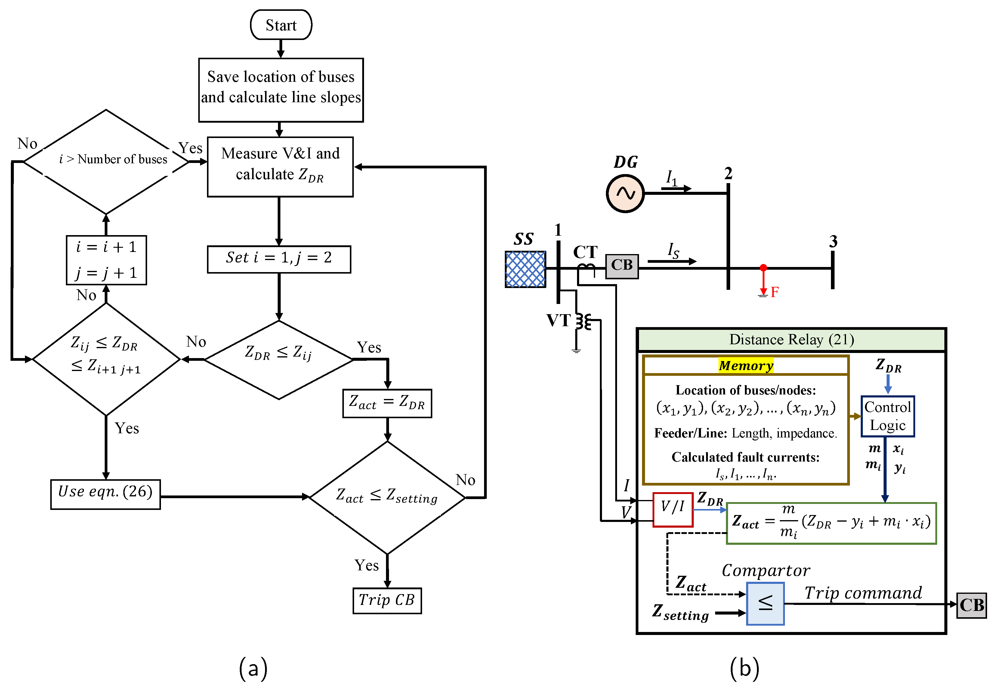
4. Proposed Methodology

Due to the infeed effect caused by one or more distributed power sources between the main source and the fault location, the measured positive-sequence impedance seen by the DR does not indicate the true positive-sequence impedance. Many solutions have been proposed to overcome this challenge. However, these solutions are either costly or have other issues related to the reliability of the protection schemes, as described above. This paper proposes a series of methods that are inexpensive, easy to implement, and do not require communication links to estimate the actual positive-sequence line impedance in the presence of one or more distributed power sources.

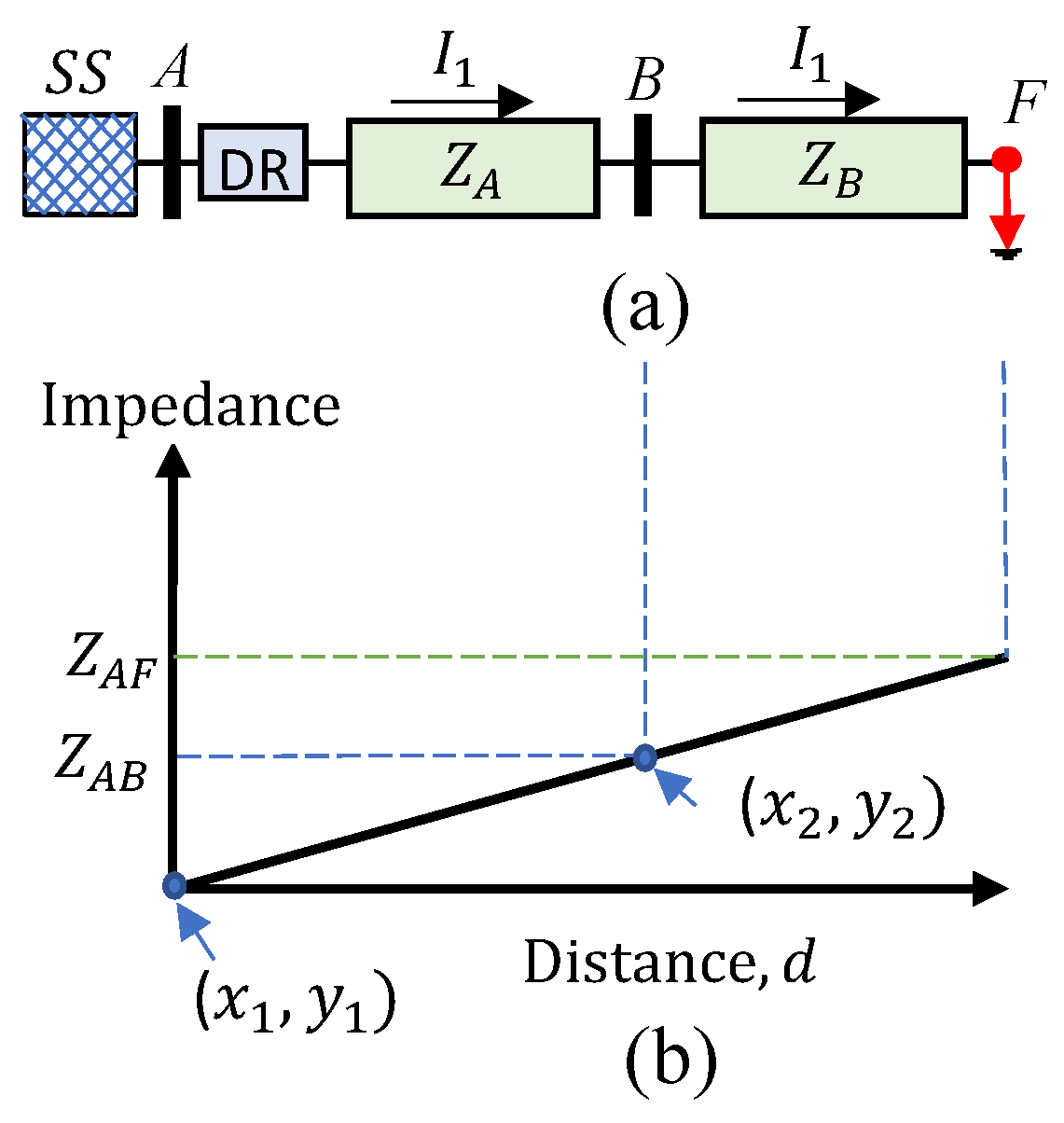
4.1. Method 1

This method requires the following data: (1) the measured impedance at the relay location; (2) the locations of the DGs; (3) the impedance and the length of the protected line; (4) fault current calculations (obtained previously from offline calculations). If the distribution feeder/transmission line has only one power source, as shown in Figure 7a, the line impedance equation as a function of distance can be written as

$$\begin{array}{cc}\hfill Z_{DR}& =m·d\hfill \end{array}$$

(18)

where $Z_{DR}$ is the positive-sequence impedance of the line/feeder corresponding to the distance d. By rearranging (18), the distance d as a function of the impedance can be represented as $d=\frac{Z_{DR}}{m}$.

A distribution feeder with a single DG is shown in Figure 8. To develop the proposed method, it is assumed that each line segment has a power source at each bus, except the last bus, which has one DG at its sending end and terminates in a load. For example, Line 1–2 in Figure 8 has the substation and $D{G}_1$ at its ends, but Line 2–3 terminates in a load.

The location/coordinate of the substation is assumed to be $(x_1,y_1)=(0,0)$ since the DR is located at Bus 1. The location/coordinate of $D{G}_1$ is $(x_2,y_2)$, where $x_2$ represents the distance from the DR location to the $D{G}_1$ location and $y_2$ represents the actual positive-sequence line impedance from the DR location to the $D{G}_1$ location. The distance $x_3$ from the DR location to Bus 3 is known, but, due to the infeed effect, the impedance $y_2$ does not equal the total positive-sequence to Bus 3. Therefore, the impedance $y_3$ must be calculated using the following equation:

$$y_3=Z_{DR}=Z_{12}+Z_{23}+K·Z_{23}$$

(19)

where $Z_{12}$ and $Z_{23}$ are the actual positive-sequence line impedances, K is the infeed constant ($K=\frac{I_1}{I_S}$), and $I_S$ and $I_1$ are the fault current contributions from the substation and $D{G}_1$ (respectively) for the case of a fault at Bus 3. The fault currents $I_S$ and $I_1$ for a 3LG fault can be calculated using the following fault calculations:

Step 1

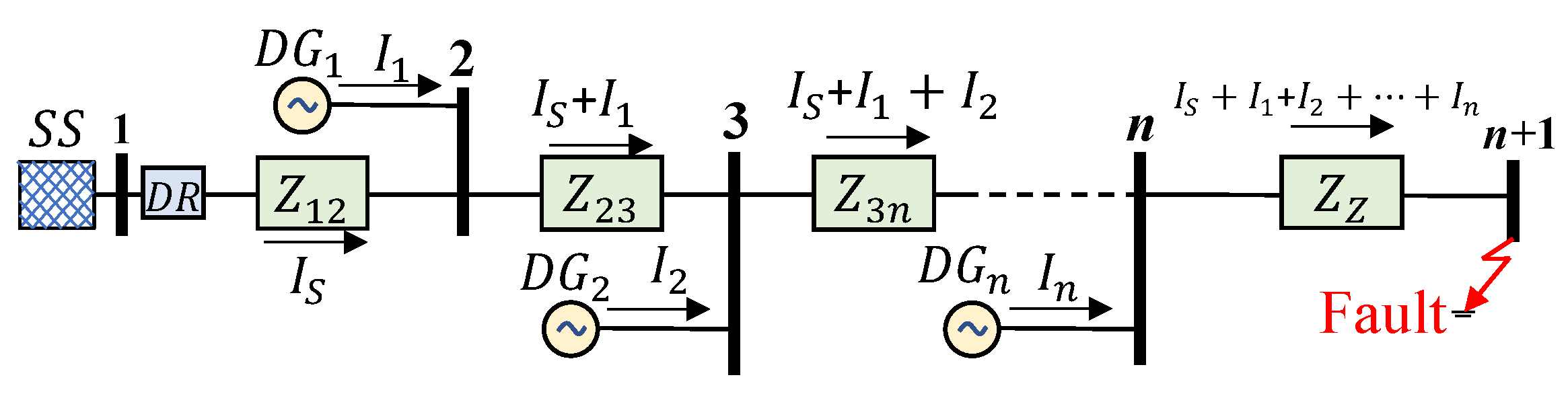
Calculation of the Thevenin impedance at the fault location. For the given system:

$$Z_{TH}^{+}=\frac{(Z_S^{+}+Z_{12}^{+})Z_{D{G}_1}^{+}}{Z_S^{+}+Z_{12}^{+}+Z_{D{G}_1}^{+}}+Z_{23}^{+}·h$$

(20)

where h is the fractional distance along the length of Line 2–3. Note that $h=1$ at Bus 3 and $h=0$ at Bus 2.

Step 2

Calculation of the fault current

$$I_{3LG}=\frac{V_f}{Z_{TH}^{+}}$$

(21)

where $V_f$ is the prefault voltage at the fault location and $Z_{TH}^{+}$ is the Thevenin impedance of the positive-sequence network at the point of the fault from Step 1.

Step 3

The fault current contributions from each source can be calculated using the current divider formula:

$$\begin{array}{cc}\hfill I_S& =I_{3LG}·\frac{Z_{D{G}_1}^{+}}{Z_S^{+}+Z_{12}^{+}+Z_{D{G}_1}^{+}}\hfill \end{array}$$

(22)

$$\begin{array}{cc}\hfill I_1& =I_{3LG}·\frac{Z_S^{+}+Z_{12}^{+}}{Z_S^{+}+Z_{12}^{+}+Z_{D{G}_1}^{+}}\hfill \end{array}$$

(23)

The actual impedance of the line can be found through leveraging the line equation that represents the impedance measured by the DR versus the distance from the fault for different configurations, i.e., the system with and without DGs. In other words, the impedance measured by DR with and without the infeed effect are compared to find the actual impedance. The measured impedance of the line in the presence of the infeed effect is formulated in (24).

$$Z_{DR}-y_2=m_2·(d-x_2)$$

(24)

where $Z_{DR}$ is the impedance measured by the DR, $x_2$ and $y_2$ represent the coordination of the first point of the faulted line segment, d is the unknown distance from the DR location up to the fault point, $m_1$ is the slope of the faulted line segment ($m_2=\frac{y_3-y_2}{x_3-x_2}$), and $x_3$ and $y_3$ are the coordinates of the remote end of the faulted line segment. Therefore, the distance to the fault can be calculated by rewriting (24) as $d=\frac{Z_{DR}-y_2}{m_2}+x_2$. Substituting d into (18), the actual positive-sequence line impedance to the fault point can be obtained:

$$Z_{act}=\frac{m}{m_2}(Z_{DR}-y_2+m_2·x_2)$$

(25)

Equation (26) is a generalization of (25) that calculates the actual impedance measured by the DR for a system with more than one DG, such as the one shown in Figure 9.

The actual impedance is given by

$$Z_{act}=\frac{m}{m_i}(Z_{DR}-y_i+m_i·x_i)$$

(26)

where $m_i$ is the slope of the faulted line, $x_i$ and $y_i$ are the coordinates of the near end of the faulted line, and i is the Bus number of the faulted segment (i.e., the near end of the faulted segment). The line segmentation data including the location of buses (i.e., x-axis in Figure 5b), impedance of the lines (i.e., y-axis in Figure 5b), and fault currents should be calculated offline and stored in the DR. To calculate the actual impedance of the line, the fault location in the system must be known. To this end, we propose an approach that iteratively compares the impedance of the line segments stored in DR with the impedance measured by the DR. The different steps of this approach are illustrated in Figure 10a. Finding the faulty section provides the impedance and distance from the DR of the underlying line, which helps to calculate the actual impedance measured by the DR according to (26). A simplified schematic diagram of Method 1 is shown in Figure 10b. The control logic in Figure 10b contains the required equations to calculate the infeed constant, K, the line slope for each line segment, and the proposed logic steps to determine the faulted segment of the line, as explained in Figure 10a.

As an example, consider the simple distribution feeder shown in Figure 11. Assume that the length of Line $AB$ is 2.5 km and $Z_A$ = 2.5 $\Omega$ and the length of Line $BC$ is 4.5 km and $Z_B$ = 4.5 $\Omega$. For a 3LG bolted fault at point C, $I_S$ and $I_1$ are $0.176\phase{{80.02}^{\circ }}$ kA and $1.576\phase{-{9.88}^{\circ }}$ kA, respectively. Therefore, the impedance measured by the DR at Bus A can be calculated using (8).

$$\begin{array}{ccc}\hfill Z_{DR}& =& Z_A+Z_B+K·Z_B\hfill \\ & =& 2.5+4.5+(8.93\phase{-{89.9}^{\circ }})·4.5\hfill \\ & =& 40.8\phase{-{80.02}^{\circ }}\Omega \hfill \end{array}$$

where K is $\frac{I_1}{I_S}=8.93\phase{-{89.9}^{\circ }}$. Note that the DR at Bus A measures an impedance of 40.8$\phase{-{80.02}^{\circ }}\Omega$ for a fault at C. This is larger than the actual impedance from A to C, which is only 7 $\Omega$. Based on the proposed approach, the feeder’s actual impedance to the fault location can be calculated:

$$\begin{array}{cc}\hfill m& =\frac{2.5-0}{2.5-0}=1\hfill \\ \hfill m_1& =\frac{40.8\phase{-{80.02}^{\circ }}-2.5}{7-2.5}=8.988\phase{-{83.51}^{\circ }}\hfill \end{array}$$

$$\begin{array}{ccc}\hfill Z_{act}& =& \frac{m}{m_1}(Z_{DR}-y_1+m_1{x}_1)\hfill \\ & =& \frac{1}{m_1}(40.8\phase{-{80.02}^{\circ }}-2.5+m_1·2.5)=7\Omega \hfill \end{array}$$

which is equal to the actual impedance of the feeder to the faulty point. It is notable that the infeed effect has no impact on the calculation.

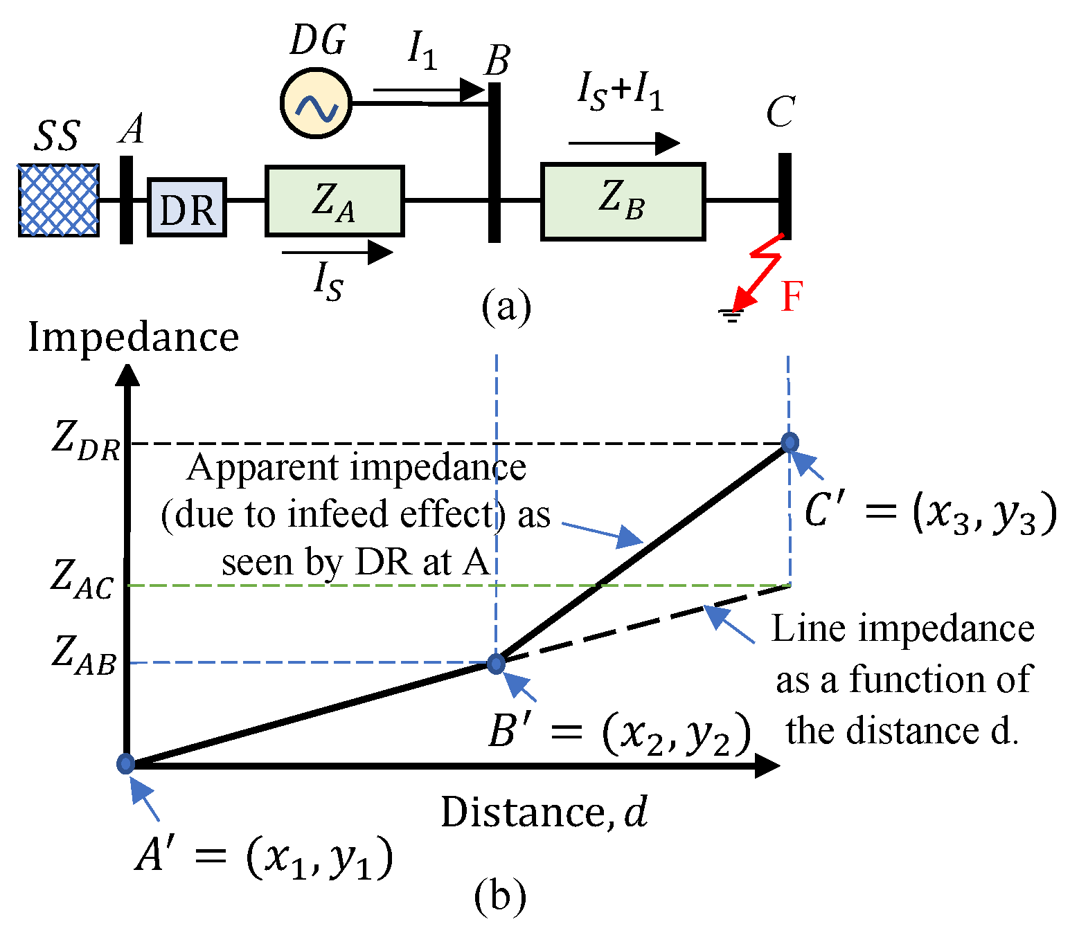
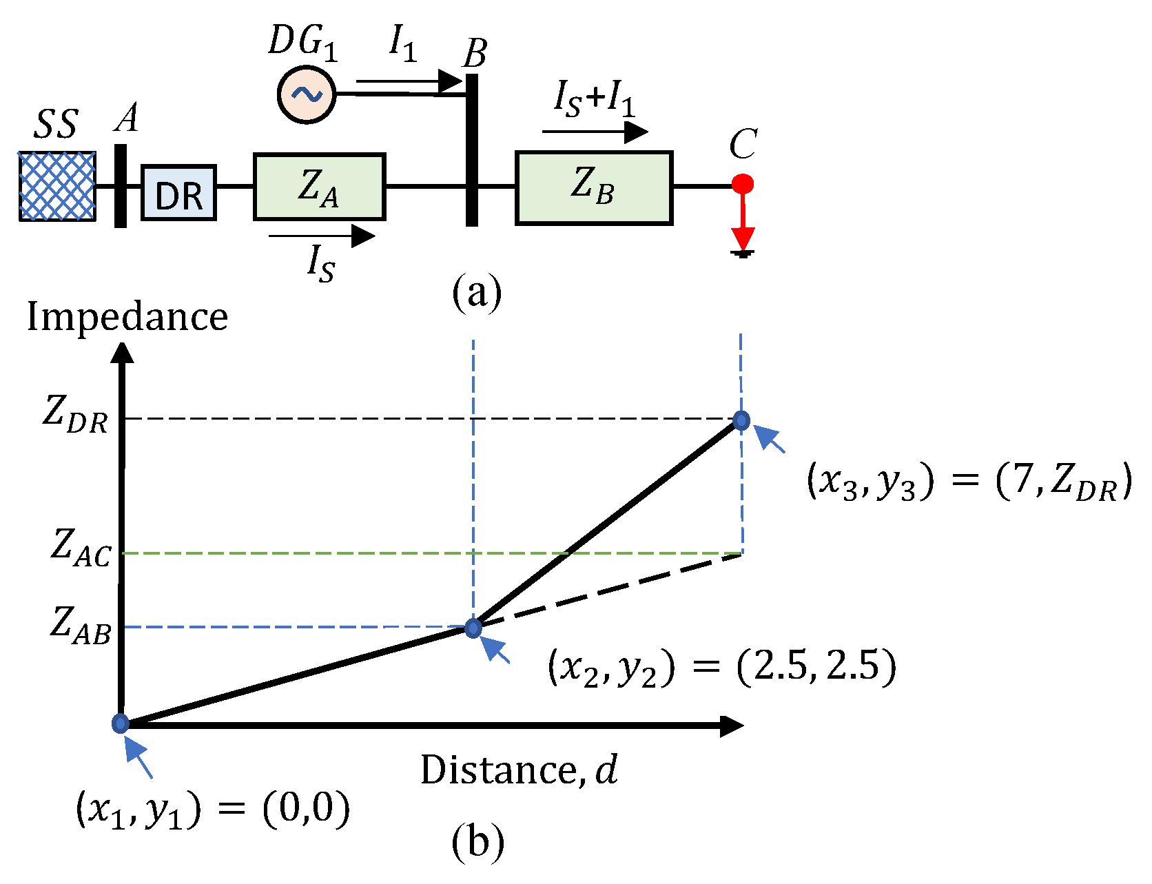
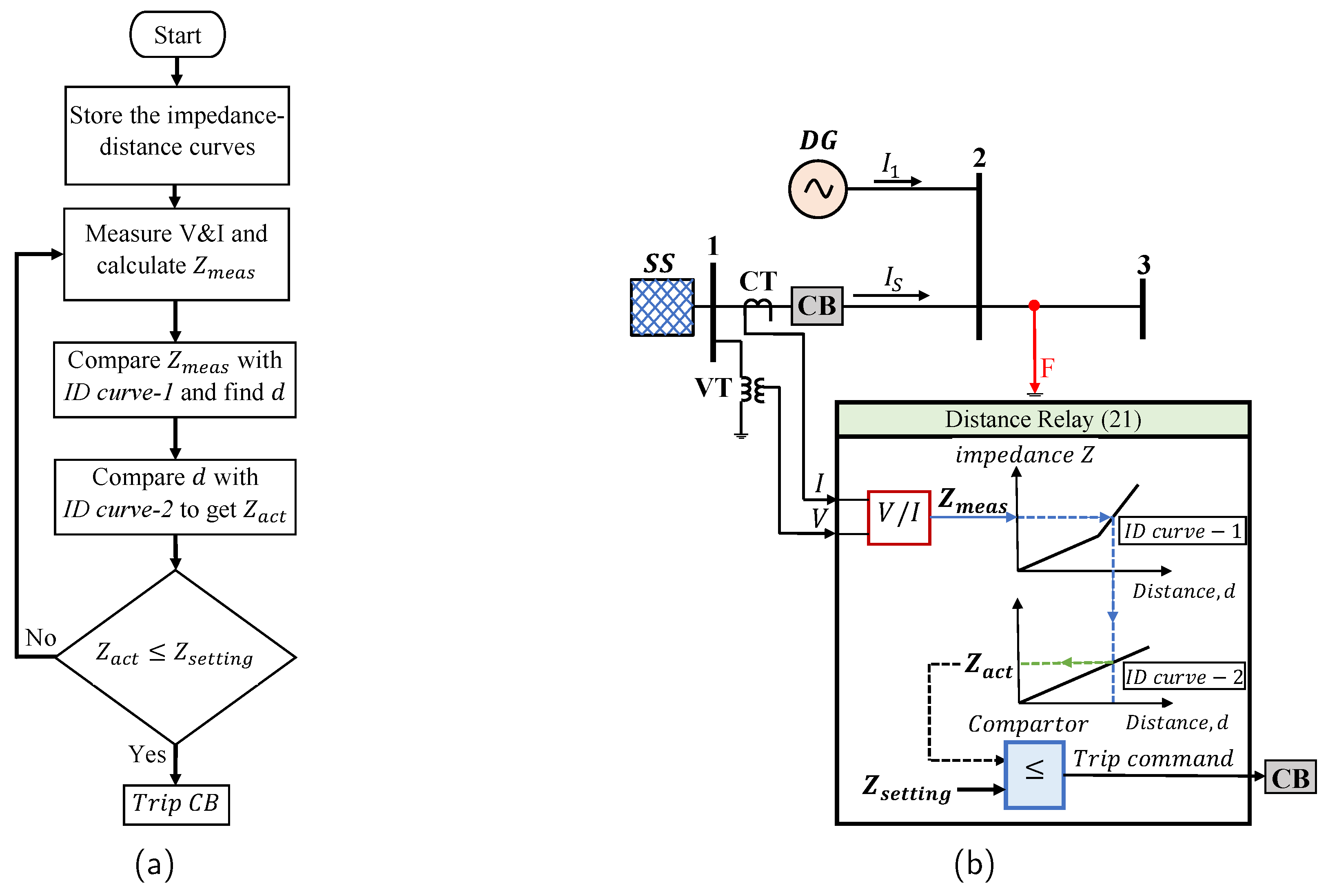
4.2. Method 2

Method 2 is based on creating two impedance–distance (ID) curves, similar to the plot in Figure 5b. The first ID curve (ID Curve 1) represents the relation between the impedance and the distance of the feeder with DGs, whereas the second ID curve (ID Curve 2) represents the impedance–distance relation of the same feeder with one power source (i.e., the main source at the beginning of the feeder/line). The impedance–distance curves should be created offline and stored in the DR. Data storage and offline calculations (even the online calculations if necessary) are not difficult for modern relays that contain large memories and advanced processors. To find the actual line impedance, $Z_{act}$, the measured impedance, $Z_{meas}$, should be compared with the ID Curve 1 to find the corresponding value of the distance. Then, the distance value is compared with the ID Curve 2 to get $Z_{act}$, as shown in Figure 12. In the case of a 3LG fault, the following steps illustrate the plotting of the line segment $B^{\prime }{C}^{\prime }$ in Figure 5b:

Step 1

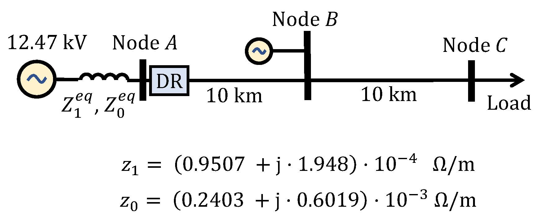
Calculation of the Thevenin impedance at the fault location. For the given system,

$$Z_{TH}^{+}=\frac{(Z_S^{+}+Z_A^{+})Z_{DG}^{+}}{Z_S^{+}+Z_A^{+}+Z_{DG}^{+}}+Z_B^{+}·d$$

(27)

where d is the fractional distance along the length of feeder/line. Note that $d=1$ at Bus C and $d=0$ at Bus B. $Z_S^{+}$ and $Z_{DG}^{+}$ are the positive-sequence impedances of the substation and DG, respectively. $Z_A^{+}$ and $Z_B^{+}$ are the positive-sequence impedances of Line $AB$ and Line $BC$, respectively.

Step 2

Calculation of the fault current as

$$I_{3LG}=\frac{V_f}{Z_{TH}^{+}}$$

(28)

where $V_f$ is the prefault voltage at fault location and $Z_{TH}^{+}$ is the Thevenin impedance of the positive-sequence network at the point of the fault from Step 1.

Step 3

The fault current contributions from each power source can be calculated using the current divider formula as follows

$$\begin{array}{cc}\hfill I_S& =I_{3LG}·\frac{Z_{DG}^{+}}{Z_S^{+}+Z_A^{+}+Z_{DG}^{+}}\hfill \end{array}$$

(29)

$$\begin{array}{cc}\hfill I_1& =I_{3LG}·\frac{Z_S^{+}+Z_A^{+}}{Z_S^{+}+Z_A^{+}+Z_{DG}^{+}}\hfill \end{array}$$

(30)

Step 4

Calculation of the infeed constant, $K=\frac{I_1}{I_S}$.

Step 5

Calculation of the impedance value corresponding to the value of d using the following equation

$$\begin{array}{cc}\hfill Z_{DR}& =Z_A^{+}+(1+K)Z_B^{+}·d\hfill \end{array}$$

(31)

Step 6

Changing the value of d in descending order (in small steps) from 1 to 0 and repeating Steps 1–5 for each d value.

Step 7

Plotting the impedance vs. distance curve.

The flowchart and the simplified schematic diagram of the proposed Method 2 are presented in Figure 12a,b, respectively.

4.3. Method 3

This method has the advantage of not requiring any offline calculations and is only based on the local measurements. It also requires the location and impedance of the infeed source to calculate the location of the fault. This data, in addition to the impedance and length of the feeder/line, which are usually known and stored in the DR as “inputs”, can be used to locate the fault without any need for measurements from the remote source. Figure 13a is used to illustrate the principle of this method.

The system in Figure 13a consists of two sources at Buses 1 and 2. The main source, $SA$, is connected to Bus 1 and the second source, $SB$, is connected to Bus 2. $SB$ can be either a strong source or a weak source. A strong source may be a feeder from another substation or a large synchronous generator, whereas a weak source may be an inverter-based resource (IBRs), such as solar or wind power [23]. To clarify how the proposed method works, we explain it for the “strong source” case under two fault types: 3LG fault and SLG faults.

4.3.1. 3LG Fault

For a 3LG fault, as shown in Figure 13a, fault currents from $SA$ and $SB$ contribute to the total fault current. Each fault current is a positive-sequence current because the fault is a symmetrical fault. The per-phase equivalent circuit of the system is shown in Figure 13b. The impedance measured by the DR can be calculated as

$$Z_{DR}=Z_1+Z_2·d·(1+\frac{I_2}{I_1})$$

(32)

and the 3LG fault current at fault location can be calculated as

$$I_{3LG}=\frac{V_f}{Z_{TH}^{+}}$$

(33)

where $V_f$ is the prefault voltage at the fault location. $Z_{TH}^{+}$ is the positive-sequence Thevenin impedance, which can be calculated as

$$\begin{array}{ccc}\hfill Z_{TH}^{+}& =& \frac{(Z_A^{+}+Z_1^{+})Z_B^{+}}{Z_A^{+}+Z_1^{+}+Z_2^{+}}+Z_2^{+}·d\hfill \\ & =& {\alpha }^{+}+Z_2^{+}·d\hfill \end{array}$$

(34)

Substituting (34) into (33) yields

$$I_{3LG}=\frac{V_f}{{\alpha }^{+}+Z_2^{+}·d}$$

(35)

Using the current-divider formula, the fault current contribution from $SB$ can be calculated as

$$\begin{array}{ccc}\hfill I_2& =& I_{3LG}·\frac{Z_A^{+}+Z_1^{+}}{Z_A^{+}+Z_1^{+}+Z_B^{+}}\hfill \\ & =& I_{3LG}·{\gamma }^{+}\hfill \end{array}$$

(36)

Substituting (33) into (36) yields

$$I_2=\frac{V_f}{{\alpha }^{+}+Z_2^{+}·d}·{\gamma }^{+}$$

(37)

Similarly, by substituting (37) into (32), the impedance $Z_{DR}$ is obtained:

$$Z_{DR}=Z_1^{+}+Z_2^{+}·d·\left(1+\frac{\frac{V_f}{{\alpha }^{+}+Z_2^{+}·d}·{\gamma }^{+}}{I_1}\right)$$

(38)

Solving (38) for d yields two possible solutions:

$$d_1,d_2=-\frac{I_1{Z_1}^{+}-I_1{Z}_{DR}+I_1{\alpha }^{+}+V_f{\gamma }^{+}\mp \beta }{2·I_1·{Z_2}^{+}}$$

(39)

where

$$\beta =\sqrt{{I_1}^2·({(Z_1^{+})}^2+Z_{DR}(-2Z_1^{+}+Z_{DR}+2{\alpha }^{+})+{({\alpha }^{+})}^2)+I_1·(-2Z_1^{+}\alpha +V_f{\gamma }^{+}·(2Z_1^{+}-2Z_{DR}+2\alpha ))+{V_f}^2{({\gamma }^{+})}^2}$$

(40)

Equation (39) has two solutions with different signs in which only the positive one ($d_2$ in this case) would be valid. The distance from the $SB$ location to the fault location is calculated using (39). Thus, the actual positive-sequence impedance from the DR location to the fault location can be calculated as

$$Z_{DR}^{act}={Z_1}^{+}+{Z_2}^{+}·d_2$$

(41)

Therefore, the per-unit distance, x, from the DR location to the fault location is

$$x=\frac{Z_{DR}^{act}}{{Z_1}^{+}+{Z_2}^{+}}$$

(42)

4.3.2. SLG Fault

The SLG fault is the most common fault that occurs in electrical networks in general and in overhead lines in particular. The SLG fault, along with line-to-line (LL) and line-to-line-to-ground (LLG) faults, are called unbalanced faults. Symmetrical components must be used for solving unbalanced faults.

The positive-sequence Thevenin impedance viewed from the fault location can be computed using (34). The negative-sequence Thevenin impedance is usually equal to the positive-sequence Thevenin impedance. Thus, it can be written as

$$\begin{array}{ccc}\hfill Z_{TH}^{-}& =& \frac{(Z_A^{-}+Z_1^{-})Z_B^{-}}{Z_A^{-}+Z_1^{-}+Z_2^{-}}+Z_2^{-}·d\hfill \\ & =& {\alpha }^{-}+Z_2^{-}·d\hfill \end{array}$$

(43)

The zero-sequence Thevenin impedance is

$$\begin{array}{ccc}\hfill Z_{TH}^0& =& \frac{(Z_A^0+Z_1^0)Z_B^0}{Z_A^0+Z_1^0+Z_2^0}+Z_2^0·d\hfill \\ & =& {\alpha }^0+Z_2^0·d\hfill \end{array}$$

(44)

The symmetrical components of the fault current are

$${I_f}^0={I_f}^{+}={I_f}^{-}=\frac{V_f}{{Z_{TH}}^0+{Z_{TH}}^{+}+{Z_{TH}}^{-}}$$

(45)

The fault current is

$$I_f=3{I_f}^0=\frac{3V_f}{{Z_{TH}}^0+{Z_{TH}}^{+}+{Z_{TH}}^{-}}$$

(46)

Applying current-divider formula, the symmetrical components of the fault current contribution from $SB$ can be expressed as

$$\begin{array}{ccc}\hfill I_2^0& =& \frac{Z_A^0+Z_1^0}{Z_A^0+Z_1^0+Z_B^0}·I_f^0\hfill \\ & =& {\gamma }^0·I_f^0\hfill \end{array}$$

(47)

$$\begin{array}{ccc}\hfill I_2^{+}& =& \frac{Z_A^{+}+Z_1^{+}}{Z_A^{+}+Z_1^{+}+Z_B^{+}}·I_f^{+}\hfill \\ & =& {\gamma }^{+}·I_f^{+}\hfill \end{array}$$

(48)

$$\begin{array}{ccc}\hfill I_2^{-}& =& \frac{Z_A^{-}+Z_1^{-}}{Z_A^{-}+Z_1^{-}+Z_B^{-}}·I_f^{-}\hfill \\ & =& {\gamma }^{-}·I_f^{-}\hfill \end{array}$$

(49)

Therefore, the fault current in phase A is

$$I_2={I_2}^0+{I_2}^{+}+{I_2}^{-}=3{I_2}^{+}$$

(50)

Substituting for $I_2$ in the infeed constant, $K=\frac{I_2}{I_1}$, yields

$$\begin{array}{ccc}\hfill K& =& \frac{3{I_2}^{+}}{I_1}\hfill \\ & =& \frac{3{\gamma }^{+}{I}_f^{+}}{I_1}\hfill \\ & =& \frac{\frac{3·V_f·{\gamma }^{+}}{{\alpha }^0+Z_2^0·d+{\alpha }^{+}+Z_2^{+}·d+{\alpha }^{-}+Z_2^{-}·d}}{I_1}\hfill \end{array}$$

(51)

$Z_{DR}$ can be expressed based on d by substituting (51) into (38),

$$Z_{DR}=Z_1^{+}+Z_2^{+}·d·\left(1+\frac{\frac{3·V_f·{\gamma }^{+}}{{\alpha }^0+Z_2^0·d+{\alpha }^{+}+Z_2^{+}·d+{\alpha }^{-}+Z_2^{-}·d}}{I_1}\right)$$

(52)

Solving for d yields

$$d=-\frac{I_1{Z}_2^{-}{Z}_1^{+}\mp \sqrt{I_1^2[a+2Z_2^{-}(b-c-d+e+f+g)+h-i-j+k+L+m)]+r+s}+v}{2I_1{Z}_2^{+}(Z_2^0+Z_2^{+}+Z_2^{-})}$$

(53)

where

$$\begin{array}{cc}\hfill a& ={(Z_2^{-})}^2·({(Z_2^{+})}^2-2Z_1^{+}{Z}_{DR}+Z_{DR}^2)\hfill \end{array}$$

(54)

$$\begin{array}{cc}\hfill b& ={(Z_1^{+})}^2·(Z_2^{+}+Z_2^0)\hfill \end{array}$$

(55)

$$\begin{array}{cc}\hfill c& =Z_1^{+}{Z}_2^{+}·(2Z_{DR}+{\alpha }^0+{\alpha }^{+}+{\alpha }^{-})\hfill \end{array}$$

(56)

$$\begin{array}{cc}\hfill d& =2Z_1^{+}{Z}_2^0{Z}_{DR}\hfill \end{array}$$

(57)

$$\begin{array}{cc}\hfill e& =Z_2^{+}{Z}_{DR}^2\hfill \end{array}$$

(58)

$$\begin{array}{cc}\hfill f& =Z_2^{+}{Z}_{DR}{\alpha }^{-}\hfill \end{array}$$

(59)

$$\begin{array}{cc}\hfill g& =Z_{DR}(Z_2^{+}({\alpha }^0+{\alpha }^{+})+Z_2^0{Z}_{DR})\hfill \end{array}$$

(60)

$$\begin{array}{cc}\hfill h& ={(Z_1^{+})}^2·({(Z_2^{+})}^2+2Z_2^{+}{Z}_2^0+{(Z_2^0)}^2)\hfill \end{array}$$

(61)

$$\begin{array}{cc}\hfill i& =2Z_1^{+}{(Z_2^{+})}^2·(Z_{DR}+{\alpha }^0+{\alpha }^{+}+{\alpha }^{-})\hfill \end{array}$$

(62)

$$\begin{array}{cc}\hfill j& =2Z_1^{+}{Z}_2^{+}{Z}_2^0·(2Z_{DR}+{\alpha }^0+{\alpha }^{+}+{\alpha }^{-})\hfill \end{array}$$

(63)

$$\begin{array}{cc}\hfill k& =Z_{DR}·(-2Z_1^{+}{(Z_2^0)}^2)+{(Z_2^{+})}^2·(Z_{DR}+2({\alpha }^0+{\alpha }^{+}+{\alpha }^{-}))\hfill \end{array}$$

(64)

$$\begin{array}{cc}\hfill L& ={(Z_2^{+})}^2·({({\alpha }^{-})}^2+2{\alpha }^{-}{\alpha }^{+}+2{\alpha }^{-}{\alpha }^0+{({\alpha }^{+})}^2+2{\alpha }^{+}{\alpha }^0+{({\alpha }^0)}^2)\hfill \end{array}$$

(65)

$$\begin{array}{cc}\hfill m& =2Z_2^{+}{Z}_2^0·(Z_{DR}^2+Z_{DR}({\alpha }^0+{\alpha }^{+}+{\alpha }^{-})+{(Z_2^0)}^2{Z}_{DR}^2\hfill \end{array}$$

(66)

$$\begin{array}{cc}\hfill r& =6I_1{V}_f{\gamma }^{+}·(Z_2^{-}{Z}_2^{+}(Z_1^{+}-ZDR)+{(Z_2^{+})}^2(Z_1^{+}-Z_{DR}+{\alpha }^0+{\alpha }^{+}+{\alpha }^{-})\hfill \end{array}$$

(67)

$$\begin{array}{cc}\hfill s& =Z_2^{+}{Z}_2^0(Z_1^{+}-Z_{DR}))+9V_f^2{(Z_2^{+})}^2{({\gamma }^{+})}^2\hfill \end{array}$$

(68)

$$\begin{array}{cc}\hfill v& =I_1[Z_1^{+}(Z_2^{+}+Z_2^0)-Z_{DR}(Z_2^0+Z_2^{+}+Z_2^{-})+Z_2^{+}({\alpha }^0+{\alpha }^{+}+{\alpha }^{-})]+3V_f{Z}_2^{+}{\gamma }^{+}\hfill \end{array}$$

(69)

Equation (53) has two solutions with different signs in which only the positive one, $d_2$, is valid. Moreover, it is important to note that $Z_{DR}$ is the corrected measured impedance, as explained in Section 3.3. The distance from the $SB$ location to the fault point is calculated using (53). Thus, the actual positive-sequence impedance from the DR location to the fault location can be calculated as

$$Z_{DR}^{act}={Z_1}^{+}+{Z_2}^{+}·d_2$$

(70)

Therefore, the per-unit distance, x, from the DR location up to the fault location is

$$x=\frac{Z_{DR}^{act}}{{Z_1}^{+}+{Z_2}^{+}}$$

(71)

The flowchart and the simplified schematic diagram of the proposed Method 3 are presented in Figure 14a,b, respectively.

5. Simulation Results

A comparison of the three proposed methods including discussion is given in this section.

5.1. Test System Description

The radial 12.47 kV, 60 Hz distribution feeder used in the simulation analysis is shown in Figure 15. The distribution feeder has two segments; each segment is 10 km long and has the following positive and zero sequence impedances, $z_1=$$(0.9507+j·1.948)·{10}^{-4}$ $\Omega$/m, and $z_0=$$(0.2403+j·0.6019)·{10}^{-3}$ $\Omega$/m. The substation is fed by an interconnected transmission grid through a step-down distribution transformer. The upstream transmission grid and the distribution transformer are represented by a Thevenin equivalent voltage source with positive and zero sequence impedances of $Z_1^{eq}=0.298\phase{{89.9}^{\circ }}$ $\Omega$ and $Z_0^{eq}=0.233\phase{{89.9}^{\circ }}$ $\Omega$ respectively. A 12.47 kV power source is also connected to the feeder at Node B, which is 10 km from the substation or DR location. The power source could be any type of strong power source, such as a synchronous generator, etc. In this simulation, we intentionally consider a larger power source at Node B, i.e., 12.47 kV with 553.8 MVA short-circuit power, in order to have a power source with a higher infeed current contribution during the fault. The feeder is protected by the DR with mho characteristics phase and ground elements at the head of the line (i.e., at Node A). The studied distribution system is modeled using PSCAD™/EMTDC™ [24].

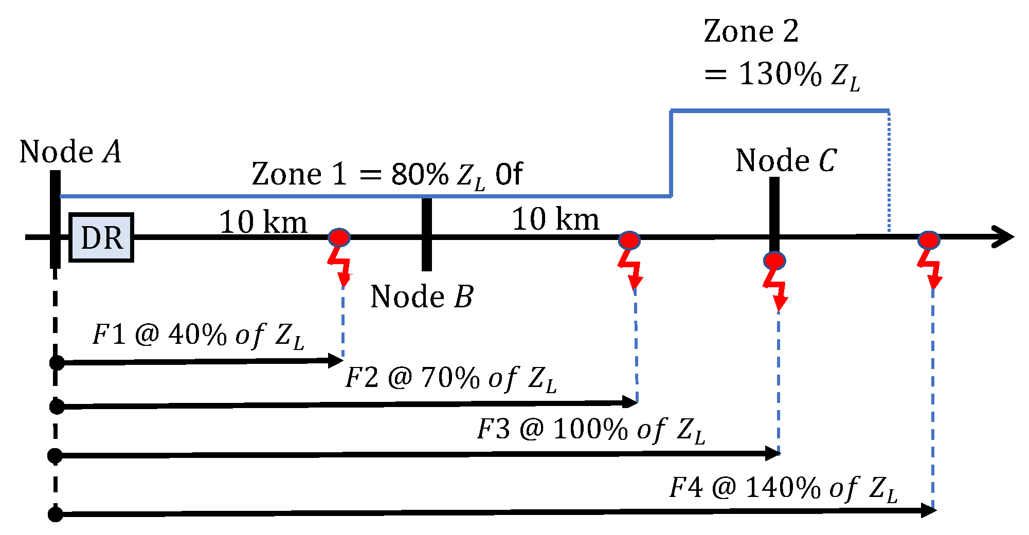
5.2. Distance Relay Settings

Two zones are set to cover the entire feeder (from Node A to Node C). Zones 1 and 2 are set to cover 80% and 130% of the positive-sequence feeder impedance, respectively. The positive-sequence line impedance is $4.3352\phase{{64}^{\circ }}$ $\Omega$. The first and second zone reaches are therefore $0.8\times 4.3352\phase{{64}^{\circ }}$ = $3.47\phase{{64}^{\circ }}$ $\Omega$ and $1.3\times 4.3352\phase{{64}^{\circ }}$ = 5.64 at ${64}^{\circ }$ $\Omega$, respectively. Zones 1 and 2 are shown in Figure 16 with green and blue mho characteristic in the complex impedance plane, respectively. For the faults located at 0–80% from the DR, the DR operates immediately. However in practice, fault isolation requires a few cycles (i.e., 6–18 cycles at 60 Hz or 0.1–0.3 s) depending on the relay decision-making process and the speed of the CB [20]. The operating time for Zone 2 is typically in the range of 0.4–0.5 s [25]. Therefore, the Zone 1 time delay is set to be 0.1 s, whereas the operating time for Zone 2 is 0.45 s.

The zero-sequence compensation factor $K_0$ is calculated and stored in the GDE in order to allow the reach settings to be specified in terms of positive-sequence impedance [7]. $K_0$ can be calculated using (15)

$$\begin{array}{ccc}\hfill K_0& =& \frac{Z_0-Z_1}{Z_1}=0.6647\phase{{6.38}^{\circ }}\hfill \end{array}$$

Converting the impedance from the primary side to the secondary side of the CT and VT does not have any impact on the proposed method, and thus we directly utilize the impedance on the primary side in this paper.

5.3. Study Cases

In order to carefully analyze the proposed methods, many fault scenarios with different fault locations and fault types were investigated. The case studies were selected to test the efficiency and accuracy of the proposed methods in measuring the feeder’s actual positive-sequence impedance in the event of faults at different distances along the distribution feeder inside and outside of the protection zones of the distance protection. In all of the case studies, there are two power sources: the distribution substation at the head of the distribution feeder (i.e., at Node A) and a power source connected to Node B, as shown in Figure 15. The study cases are for bolted 3LG and SLG faults at a distance of 40%, 70%, 100%, and 140% of the distribution feeder length. The fault locations and the DR scheme used in the case studies are shown in Figure 17.

5.3.1. Case I: Fault at a Distance of 40% of the Feeder’s Length

The objective of this case is to establish the effectiveness of the proposed methods in the event of a fault between the substation and the power source at Node B (i.e., within the boundaries of Zone 1). The impedance seen by the DR for a 3LG fault located at $F1$ (see Figure 17 for fault locations) is shown in Figure 18a. Since the infeed effect does not affect the reading of the DR, the measured impedance is correct and is the actual positive-sequence impedance between the DR location and fault location. Therefore, the Zone 1 element provides tripping with a time of 0.1 s, which is the correct function of the DR. Similarly, the impedance trajectory in the case of the SLG fault is illustrated in Figure 18b. $Z_c$ denotes the conventionally measured impedance.

5.3.2. Case II: Fault at a Distance of 70% of the Feeder’s Length

The objective of this case is to establish both the effectiveness and accuracy of the proposed methods on the DR’s measurements. The DR performance in the case of 3LG and SLG faults is shown in Figure 19a,b, respectively. We observed that the impedance measured by the conventional DR, $Z_c$, is out of the operating zones of the DR, although the fault is within the operating characteristic of Zone 1. However, the impedance measured by the proposed methods, $Z_{m1}$ (Method 1), $Z_{m2}$ (Method 2), and $Z_{m3}$ (Method 3), are all located within the Zone 1 area. Numerically, the measured impedance $Z_c$ to the fault at the DR location for a 3LG fault is 2.39 pu, rather than the actual positive-sequence impedance of 0.7 pu. By contrast, the impedance measured by the proposed methods $Z_{m1}$, $Z_{m2}$, and $Z_{m2}$ are all equal to 0.7 pu. The measured impedance $Z_c$ is 3.69 pu for a SLG fault at $F2$, while the measured impedance by the proposed methods $Z_{m1}$, $Z_{m2}$, and $Z_{m2}$ are 0.7, 0.7, and 0.68 pu, which are the same as, or close to, the actual positive-sequence impedance from the DR location to the fault point $F2$.

5.3.3. Case III: Fault at a Distance of 100% of the Feeder’s Length

In this case, the fault location is outside of Zone 1 but within the boundaries of Zone 2. As shown in Figure 20a,b, $Z_{m1}$, $Z_{m2}$, and $Z_{m3}$ trajectories move into Zone 2. However, the $Z_c$ trajectory is out of the operating zones of the DR. Therefore, $Z_{m1}$, $Z_{m2}$, and $Z_{m3}$ reflect the correct impedance trajectory. Thus, the DR trip is delayed by the time setting of Zone 2, which is set at 0.45 s. The measured $Z_c$ for a 3LG fault at $F3$ is 5.26 pu, whereas $Z_{m1}$, $Z_{m2}$, and $Z_{m3}$ are all equal to 1 pu for the same fault. Similarly, the measured $Z_c$ is 8.49 pu for SLG fault, whereas $Z_{m1}$, $Z_{m2}$, and $Z_{m3}$ are 1.0, 1.0, and 1.01 pu, which are the same as, or close to, the actual positive-sequence impedance from the DR location to the fault point $F3$.

5.3.4. Case IV: Fault at a Distance of 140% of the Feeder’s Length

The impedance trajectories seen by the DR in the case of 3LG and SLG faults at $F4$ are plotted in Figure 21a,b, respectively. In this case, the fault location is outside the operating characteristic of Zone 2. As shown in Figure 21a,b, $Z_{m1}$, $Z_{m2}$, and $Z_{m3}$ are outside Zone 2 as expected. Thus, the DR does not trip, reflecting a correct decision of the DR. The measured $Z_c$ for a 3LG fault at $F4$ is 9.09 pu, whereas $Z_{m1}$, $Z_{m2}$, and $Z_{m3}$ are all equal to 1.4 pu for the same fault. Similarly, the measured $Z_c$ is 14.84 pu for SLG fault, while $Z_{m1}$, $Z_{m2}$, and $Z_{m3}$ are 1.4, 1.4, and 1.48 pu which are the same as, or close to, the actual positive-sequence impedance from the DR location to the fault point $F4$.

The results of the different case studies are summarized in

Table 1. Distance relay performance under varying system conditions.

Fault	Fault	Zone	${\mathit{Z}}_{\mathbf{act}}$	Measured Impedance, pu
Type	Location	Protection	(pu)	${\mathit{Z}}_{\mathit{c}}$	${\mathit{Z}}_{\mathit{m}1}$	${\mathit{Z}}_{\mathit{m}2}$	${\mathit{Z}}_{\mathit{m}3}$
3LG	F1	1	0.4	0.4	0.4	0.4	0.4
	F2	1	0.7	2.39	0.7	0.7	0.7
	F3	2	1.0	5.26	1.0	1.0	1.0
	F4	Out of zones	1.4	9.09	1.4	1.4	1.4
SLG	F1	1	0.4	0.4	0.4	0.4	0.4
	F2	1	0.7	3.69	0.7	0.7	0.68
	F3	2	1.0	8.49	1.0	1.0	1.01
	F4	Out of zones	1.4	14.84	1.4	1.4	1.48

. The impedance values are in pu based on the magnitude of the positive-sequence impedance of the distribution feeder ($|Z_{base}|=4.3352\Omega$). $Z_{act}$ in Column 4 is the actual positive-sequence impedance in pu of the distribution feeder. $Z_{m1}$, $Z_{m2}$, and $Z_{m3}$, in Columns 6–8, are the measured impedances by the proposed Methods 1–3, respectively. Similar observations were made for both line–line and line–line–ground faults.

5.4. Comparison of Methods

Each of the proposed methods has its own technique for determining the location of the fault. Different features of the proposed methods including the required data and calculations, cost, and results accuracy are compared to clarify the differences between them.

• Required data and calculations: All three methods require local measurements and the system’s data in order to determine the fault location in the presence of an infeed current. In addition to the system data and local measurements, the first and second methods require the results of offline calculations in order to determine the fault location. The first method requires calculating the offline fault current values as part of the data to be stored in the DR. Similarly, the second method requires calculating offline fault currents to create ID curves. The third method has an advantage over the first two methods in that it does not require any offline calculations, and its functionality entirely depends on local measurements.
• Cost: The functionality of three methods proposed in this paper do not require the addition of any measuring or communication devices. In other words, the proposed methods do not incur any additional hardware cost to the current system.
• Accuracy of the results: One of the most important indicators of the success for any method is its accuracy. To this end, all of the proposed methods were tested using PSCAD™/EMTDC™ software. The results prove the capability of the proposed methods in locating the faults with high accuracy in the presence of an infeed effect. Method 3 is the least accurate due to its dependence purely on online measurements with no offline calculations, but the drop in accuracy may be counter-balanced by its other advantages.

A summary comparison of the proposed methods is presented in

Table 2. Comparison of the proposed methods.

Proposed	Required Data	Cost	Accuracy of
Methods	and Calculations		the Results
Method 1	Local measurements	Very low	Very high
	System data
	Offline calculations
Method 2	Local measurements	Very low	Very high
	System data
	Offline calculations
Method 3	Local measurements	Very low	High
	System data

.

6. Conclusions

Increasing the amount of renewable generation in a distribution system increases the infeed current, which challenges the current protection scheme. Three different solutions for addressing the maloperation of distance relays in power systems caused by the infeed effect are presented in this paper. Previous works that address the same issue with distance relay are either costly or have low reliability. To overcome these challenges, the methods proposed in this paper not only accurately estimate the distance to the fault in the presence of the infeed effect but also are more reliable compared to the former solutions. Furthermore, they are applicable for distance relays, in either radial distribution feeders or transmission lines. Lastly, the proposed methods do not need any peripherals, such as a communications link, to operate and are thus more economical compared to the former solutions. The accuracy of the proposed methods are examined using different case studies. The obtained results indicate the potential superiority of the proposed methods over similar proposed methods.

References

- Gonen, T. Electric Power Distribution Engineering; CRC Press: Boca Raton, FL, USA, 2015; p. 768. [Google Scholar]
- Wheeler, K.W.; Elsamahy, M.; Faried, S.O. A Novel Reclosing Scheme for Mitigation of Distributed Generation Effects on Overcurrent Protection. IEEE Trans. Power Deliv. 2018, 33, 981–991. [Google Scholar] [CrossRef]
- Tong, X.; Liu, J. Fault Processing Based on Local Intelligence. In Fault Location and Service Restoration for Electrical Distribution Systems; John Wiley & Sons: Hoboken, NJ, USA, 2016; Chapter 2; p. 32. [Google Scholar]
- El-Khattam, W.; Sidhu, T.S. Restoration of Directional Overcurrent Relay Coordination in Distributed Generation Systems Utilizing Fault Current Limiter. IEEE Trans. Power Deliv. 2008, 23, 576–585. [Google Scholar] [CrossRef]
- Singh, M.; Vishnuvardhan, T.; Srivani, S.G. Adaptive protection coordination scheme for power networks under penetration of distributed energy resources. IET Gener. Transm. Distrib. 2016, 10, 3919–3929. [Google Scholar] [CrossRef]
- Usama, M.; Mokhlis, H.; Moghavvemi, M.; Mansor, N.; Alotaibi, M.; Muhammad, M.; Bajwa, A. A Comprehensive Review on Protection Strategies to Mitigate the Impact of Renewable Energy Sources on Interconnected Distribution Networks. IEEE Access 2021, 9, 35740–35765. [Google Scholar] [CrossRef]
- Sinclair, A.; Finney, D.; Martin, D.; Sharma, P. Distance Protection in Distribution Systems: How It Assists with Integrating Distributed Resources. IEEE Trans. Ind. Appl. 2014, 50, 2186–2196. [Google Scholar] [CrossRef]
- Chang, J.; Gara, L.; Fong, P.; Kyosey, Y. Application of a multifunctional distance protective IED in a 15KV distribution network. In Proceedings of the 2013 66th Annual Conference for Protective Relay Engineers, College Station, TX, USA, 8–11 April 2013; pp. 150–171. [Google Scholar] [CrossRef]
- Enayati, A.; Ortmeyer, T.H. A novel approach to provide relay coordination in distribution power systems with multiple reclosers. In Proceedings of the 2015 North American Power Symposium (NAPS), Charlotte, NC, USA, 4–6 October 2015; pp. 1–6. [Google Scholar] [CrossRef]
- Tsimtsios, A.M.; Nikolaidis, V.C. Setting Zero-Sequence Compensation Factor in Distance Relays Protecting Distribution Systems. IEEE Trans. Power Deliv. 2018, 33, 1236–1246. [Google Scholar] [CrossRef]
- Ziegler, G. Numerical Distance Protection: Principles and Applications; John Wiley & Sons: Hoboken, NJ, USA, 2011. [Google Scholar]
- Blackburn, J.L.; Domin, T.J. Protective Relaying: Principles and Applications; CRC Press: Boca Raton, FL, USA, 2015; pp. 600–602. [Google Scholar]
- Gers, J.M.; Holmes, E.J. Protection of Electricity Distribution Networks; IET: London, UK, 2011; Volume 47. [Google Scholar]
- Biswas, S.; Centeno, V. A communication based infeed correction method for distance protection in distribution systems. In Proceedings of the 2017 North American Power Symposium (NAPS), Morgantown, WV, USA, 17–19 September 2017; pp. 1–5. [Google Scholar] [CrossRef]
- Uzubi, U.; Ekwue, A.; Ejiogu, E. Adaptive distance relaying: Solution to challenges of conventional protection schemes in the presence of remote infeeds. Int. Trans. Electr. Energy Syst. 2020, 30, e12330. [Google Scholar] [CrossRef]
- Mishra, P.; Pradhan, A.K.; Bajpai, P. Adaptive Distance Relaying for Distribution Lines Connecting Inverter-Interfaced Solar PV Plant. IEEE Trans. Ind. Electron. 2021, 68, 2300–2309. [Google Scholar] [CrossRef]
- Thakre, M.P.; Kale, V.S. An adaptive approach for three zone operation of digital distance relay with Static Var Compensator using PMU. Int. J. Electr. Power Energy Syst. 2016, 77, 327–336. [Google Scholar] [CrossRef]
- Tsimtsios, A.M.; Korres, G.N.; Nikolaidis, V.C. A pilot-based distance protection scheme for meshed distribution systems with distributed generation. Int. J. Electr. Power Energy Syst. 2019, 105, 454–469. [Google Scholar] [CrossRef]
- Anderson, P.M. Power System Protection; Wiley-IEEE Press: Piscataway, NJ, USA, 1999; p. 379. [Google Scholar]
- Kezunovic, M.; Ren, J.; Lotfifard, S. Design, Modeling and Evaluation of Protective Relays for Power Systems; Springer: Berlin/Heidelberg, Germany, 2016. [Google Scholar]
- Horowitz, S.H.; Phadke, A.G. Power System Relaying; John Wiley & Sons: Hoboken, NJ, USA, 2014; p. 111. [Google Scholar]
- Nikolaidis, V.C.; Tsimtsios, A.M.; Safigianni, A.S. Investigating Particularities of Infeed and Fault Resistance Effect on Distance Relays Protecting Radial Distribution Feeders with DG. IEEE Access 2018, 6, 11301–11312. [Google Scholar] [CrossRef]
- Jones, K.W.; Pourbeik, P.; Kobet, G.; Berner, A.; Fischer, N.; Huang, F.; Holbach, J.; Jensen, M.; O’Connor, J.; Patel, M.; et al. Impact of Inverter Based Generation on Bulk Power System Dynamics and Short-Circuit Performance; Technical Report PES-TR68; IEEE Power & Energy Society: New York, NY, USA, 2018. [Google Scholar]
- International, M.H. PSCAD Version 5.0. Winnipeg, MB, Canada. 2021. Available online: https://www.pscad.com/ (accessed on 30 July 2021).
- Ibrahim, M.A. Disturbance Analysis for Power Systems, 1st ed.; Wiley: Hoboken, NJ, USA, 2011; p. 223. [Google Scholar]