
MC-NILM: A Multi-Chain Disaggregation Method for NILM


1
School of Computer Science and Technology, Soochow University, Suzhou 215006, China
2
Jiangsu Province Software New Technology and Industrialization Collaborative Innovation Center, Nanjing 210023, China
3
School of Mechanical and Electrical Engineering, Soochow University, Suzhou 215137, China
*
Author to whom correspondence should be addressed.
Energies 2021, 14(14), 4331; https://doi.org/10.3390/en14144331
Submission received: 29 June 2021
/
Revised: 11 July 2021
/
Accepted: 14 July 2021
/
Published: 18 July 2021
(This article belongs to the Special Issue Digital Transformation in the Energy Sector: Data-Driven Analytics, Services and Business Models)
Abstract
:Non-intrusive load monitoring (NILM) is an approach that helps residents obtain detailed information about household electricity consumption and has gradually become a research focus in recent years. Most of the existing algorithms on NILM build energy disaggregation models independently for an individual appliance while neglecting the relation among them. For this situation, this article proposes a multi-chain disaggregation method for NILM (MC-NILM). MC-NILM integrates the models generated by existing algorithms and considers the relation among these models to improve the performance of energy disaggregation. Given the high time complexity of searching for the optimal MC-NILM structure, this article proposes two methods to reduce the time complexity, the k-length chain method and the graph-based chain generation method. Finally, we use the Dataport and UK-DALE datasets to evaluate the feasibility, effectiveness, and generality of the MC-NILM.
1. Introduction
Energy is the material basis for the progress and development of human society. Electricity is a very convenient way to transfer energy, and it has been adapted to a huge and growing number of uses. Nowadays, global electricity consumption is increasing year by year, and people are facing an increasingly severe energy shortage problem. The management and optimization of energy usage can effectively reduce energy consumption. Knowing the detailed usage of energy can effectively help residents optimize electric energy management. Some research [1] pointed out that disaggregated information can help householders to reduce energy consumption by 15%. Therefore, household electrical energy consumption analysis has gradually become a research field that attracts much attention.
In terms of household energy management, load monitoring is an approach that helps residents save energy. The purpose of load monitoring is to obtain power data of various appliances in the entire house. Power companies can use load monitoring approach to get information about the users’ energy consumption composition and strengthen load-side management. Such energy consumption information can guide the users to schedule the usage of the high-power non-emergency load to adjust the peak-to-valley difference and reduce network losses. Currently, researchers divide load monitoring into two categories: intrusive and non-intrusive [2]. Intrusive load monitoring uses sensors installed on each line to collect data for each appliance’s status and power. The result of this scheme is relatively accurate, but it needs to install a large number of sensors in residents’ houses with the high cost and low feasibility. Non-intrusive load monitoring (NILM) is also called energy disaggregation, which does not need to install sensors on all lines. The sensors only need to monitor the voltage, current, and other signals at the entrance of the power system, which significantly reduces the hardware cost and installation complexity. NILM can be used for home energy management systems (HEMS) and ambient assisted living (AAL) [3,4,5].
Hart first proposed the concept of NILM and its solutions in the 1990s [6]. Many researchers have proposed various solutions ever since. Ways to solve the NILM problem can be divided into low-frequency approaches and high-frequency approaches according to the sampling rate of the input signals. Low-frequency approaches use data (i.e., features) produced at rates lower than the alternating current (AC) base frequency, and high-frequency approaches use data sampled at rates higher than the AC base frequency [7]. Although more information can be extracted from high-frequency data [8], the required data acquisition equipment is more expensive. Therefore, this article studies the low-frequency approaches.
The main stages in NILM are: data collection, event detection, feature extraction, and load identification [9]. Ruzzelli et al. [10] proposed a method for NILM using the steady-state voltage information (i.e., peak value, average value, and standard deviation) and its waveform characteristics. Hassan et al. [11] used voltage-current traces for NILM and pointed out that using the combination of voltage and current traces is more straightforward to distinguish among different appliances than using voltage waveforms or current waveforms individually. Figueiredo et al. [12] proposed a non-negative tensor disaggregation method to extract features. They used the extracted features to perform energy disaggregation. Batra et al. [13] regarded NILM as a combinatorial optimization problem and proposed an algorithm to solve this problem. Some researchers are inspired by speech recognition and used hidden Markov models and their variants to solve this problem [14,15]. Some researchers [16,17] have also proposed event-based disaggregation methods. They first extracted the rising/falling edge characteristics. They then used different classification methods to classify the features to infer the appliances’ power, including support vector machines (SVM), fuzzy logic (FL), Naive Bayesian (NB), K-means, and decision tree (DT).
In recent years, with the continuous breakthroughs in computer vision, speech recognition, natural language processing, and other fields using deep learning, many scholars have also begun to use deep learning methods to solve the NILM problem. In 2015, Kelly et al. [18] used long short-term memory (LSTM), denoising autoencoder (DAE), and other deep neural networks to solve the NILM problem with low-frequency signals. Nascimento [19] used convolutional neural network (CNN) and recurrent neural network (RNN) for energy disaggregation. Kim et al. [20] applied gated recurrent unit (GRU) to NILM. Zhang et al. [21] proposed a sequence-to-point (Seq2point) method, which used mains data to generate the model’s input through a sliding window. The model’s output is the estimated power of the target appliance corresponding to the input data at the middle of the time. Pan et al. [22] applied generative adversarial network (GAN) to NILM and proposed a sequence-to-subsequence (Seq2subseq) method based on conditional GAN (cGAN). Puente et al. [23] proposed an unsupervised disaggregation method, which can identify the behavior of each appliance from mains power data through soft computing technology. The method proposed in this work establishes a box model composed of a sequence of rectangles of different heights (powers) and widths (times) to detect power changes. Piccialli et al. [24] combined the power and status information of the appliance and used a deep neural network that combines a regression sub-network with a classification sub-network to solve the NILM problem. The deep neural network used regression sub-network to infer the appliance’s power and classification sub-network to infer the state of the appliance. This work also added the attention mechanism to the deep neural network to improve the generalization ability of the neural network. Lee et al. [25] proposed an auto-encoder compression model based on the frequency selection method for NILM in the Internet of Things (IoT) environment, which can improve the reconstruction quality while maintaining the compression ratio (CR).
All of the above methods regard the models used to infer different appliances as independent models, and there is no correlation between the models. Jia et al. [26] proposed a tree structure model (treeCNN) for NILM, which considers the relation of models for different target appliances. TreeCNN placed different models as sub-models in the tree structure nodes to generate an overall model, which maintained the relative independence of each sub-model and established a connection between them. Although this method is called a tree structure method, the sub-models in treeCNN are all in a chain. Therefore, in this article, we call this disaggregation method the single-chain disaggregation method for NILM (SC-NILM). In [26], a brute-force method and a greedy method are proposed to obtain the single-chain. For the convenience of description, in this article, we will call them Opt-SC and Gre-SC, respectively. Batra et al. [27] developed a non-intrusive load monitoring toolkit (NILMTK) to facilitate researchers to use existing public datasets and quickly implement their ideas. At present, the toolkit integrates a total of 12 NILM algorithms.
When performing energy disaggregation, most researchers input mains data into a specific model, and the model outputs the inferred value of the power of the target appliance. In other words, inferring the power of multiple target appliances requires many independent models. In this article, we use the existing model for individual target appliances as a sub-model. Furthermore, multiple sub-models constitute multiple chains. The output of the end node of each chain is an inferred value of the power of the different appliances. The chains constitute an overall model, which we call the MC-NILM. Due to the high time cost of using the brute-force method to obtain the MC-NILM with the best performance, this article proposes two solutions to reduce complexity. The first approach is to reduce the total number of MC-NILM by limiting the maximum length of chains. This solution can reduce the search space when using the brute-force method to search for the best-performing MC-NILM. The second approach is to evaluate the relative position of each pair of sub-models in a chain for a target appliance and use this information to guide the searching of chain structure with a graph-based algorithm (GBA). We tested MC-NILM on two public datasets, Dataport and UK-DALE, and used different metrics to evaluate performance. Experimental results show that our MC-NILM is better than several baselines, including Opt-SC and Gre-SC. The performance gap between our chain searching methods and the exhaustive search is close.
The main contributions of this paper are as follows:
- (1)
- We proposed a multi-chain energy disaggregation method that considers the relationship between appliances for energy disaggregation and constructs a separate energy disaggregation chain for each appliance;
- (2)
- We proposed two methods to reduce the complexity of the search for MC-NILM structure;
- (3)
- Our experimental results demonstrated that the MC-NILM method is a general framework to leverage the existing NILM algorithms as sub-models and improve the overall performance of the original algorithms.
2. NILM Problem Statement
NILM is a computational technique for estimating the power of individual appliances from the data obtained from a single meter that measures total power consumption [18,28].
Use Y to represent the household’s observed mains power from time 1 to T, and Y can be represented as follows:
The set of N appliances that need to infer power is defined as A,
The power of the appliance can be expressed as
In addition, the mains also includes some appliances that do not need to infer power. The power of these appliances is added together as a whole as an unconcerned appliance U,
In addition, the mains data also contains noise, and is used to represent the noise in the mains at time t. The relationship between mains and its components can be expressed as
The purpose of NILM is to reconstruct the from Y.
3. MC-NILM
3.1. Overview
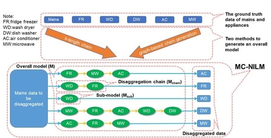
This article proposes the MC-NILM based on the following idea. When inferring the power of the target appliance , the data of other appliances in the mains acts as interference. If the data of other appliances are removed from the input data as much as possible, the power of can be inferred from mains more easily. This article uses an iterative method with a chain structure to remove the power of non-target appliances from the mains gradually. The function of nodes in the chain except the end node is to infer the power of other appliances except . We subtract the inferred power from the input data of the node as the input data of the subsequent node. The output of the end node is the inferred power of the target appliance . This method simplifies the input data of the end node and improves the ability of the end node to infer the power of . The permutation of other appliances in the chain affects the inferred output about . Since each appliance has its unique characteristics and energy consumption pattern, the optimal chains for different target appliances are also different. Therefore, we need to use multiple chains to infer the power of multiple target appliances, which is called MC-NILM. At present, the most similar to our idea is treeCNN [26]. However, the treeCNN uses a single chain for all target appliances (SC-NILM). As will be shown later, our proposed MC-NILM method can achieve better performance. Figure 1 shows a schematic diagram of the three disaggregation schemes. They are (a) the independent method adopted by most researchers, (b) the SC-NILM proposed in [26], (c) the MC-NILM proposed in this article. Figure 1 uses the five appliances studied in [26] to illustrate the three schemes.
In MC-NILM, each appliance has its disaggregation chain. The set of multiple chains is denoted by , where denotes the disaggregation chain for . is an ordered list of sub-models. Furthermore, we use to represent a sub-model used to infer the power of from the power of the corresponding components in , where Z is a collection of all mains components including target appliances, unconcerned appliances and noise, is a subset of A, represents the set Z subtract the power of appliances in set , i is the index of the appliance. In particular, when is an empty set, is abbreviated as Z, and represents the set formed by taking out the appliance from the set Z. In addition, this article uses to represent the performance of .
The overall process of MC-NILM to infer the power of the target appliances is as follows:
- We divide the whole dataset into three parts: sub-model training dataset , multi-chain structure search dataset , and performance testing dataset ;
- We use to train multiple sub-models, which can be used to form disaggregation chains;
- We use to search for the optimal multi-chain model for the target appliances, which is denoted by as a whole;
- We evaluate the performance of on .
Next, we will introduce the details of the MC-NILM.
3.2. Sub-Model Training
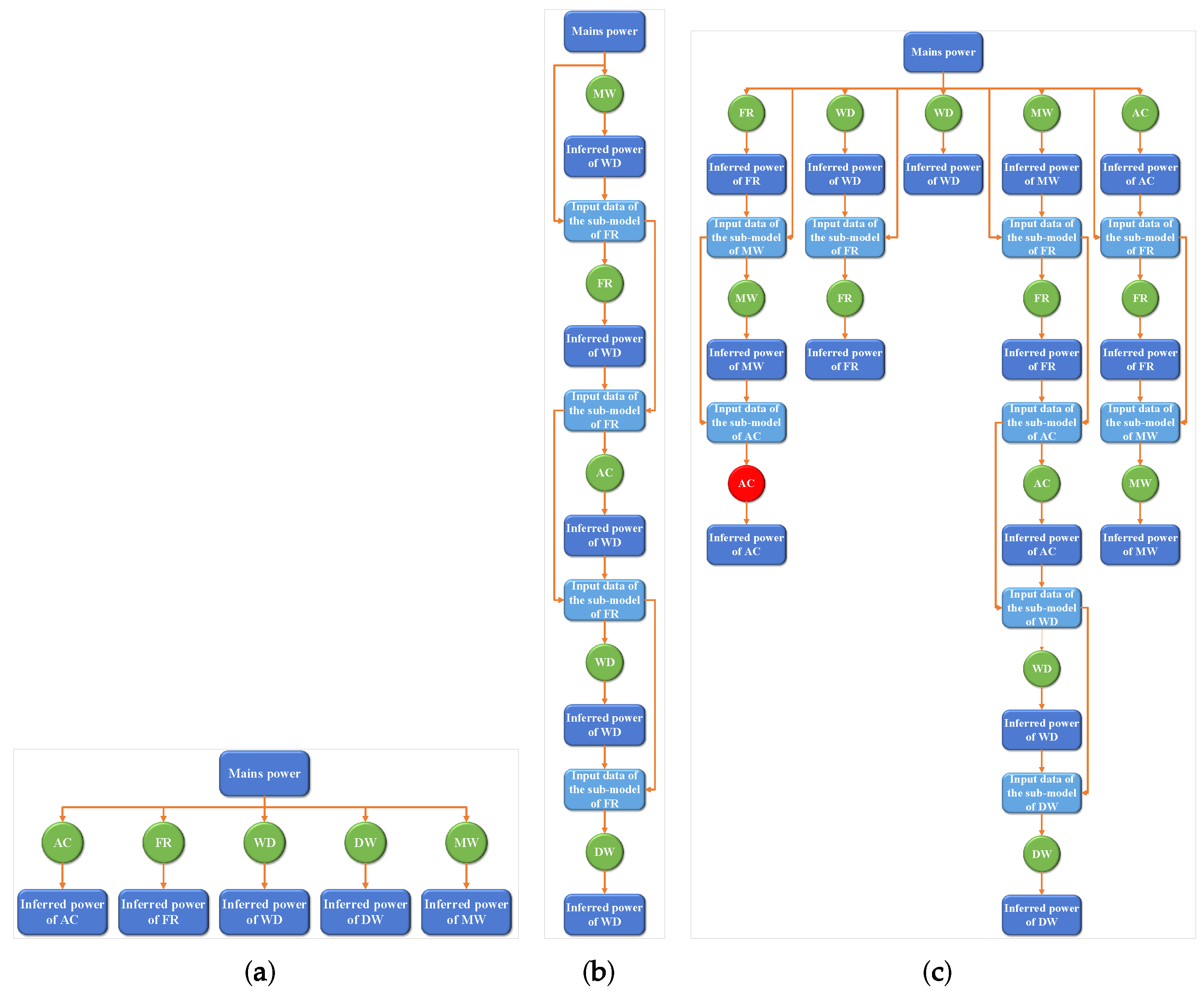
The MC-NILM proposed in this article consists of sub-models that can be created by any existing NILM method. As mentioned in the previous subsection, the first step in creating an MC-NILM is to train sub-models. For ease of description, we use the red node of an air conditioner (AC) in Figure 1c to illustrate the training process of the sub-model. In the training stage of the sub-model, the feature is ground truth power data obtained by subtracting the fridge freezer (FR) and microwave (MW) power data from the mains data. The label is the ground truth power data of the AC. In the sub-model’s inference stage, the sub-model’s input is the data obtained by gradually subtracting the output value of the node before the sub-model from the mains. The input of the sub-model is the inferred value of the power of the FR and the MW, and the output is the inferred value of the power of AC. This approach can reduce the complexity of the input data of the sub-model and reduce the difficulty of the sub-model training process.
3.3. Energy Disaggregation in a Chain
Figure 1c illustrates an example of the MC-NILM. When inferring the power of the target appliances, the MC-NILM uses different chains to infer the power of different target appliances. The input for all chains is the mains power. Along a particular chain, the powers of several other appliances except for the target one are inferred with sub-models and extracted from the mains power iteratively. The output at the end of the chain is then the inferred power of the target appliance. In this way, due to its multi-chain structure, the MC-NILM can obtain power inference data for each target appliance through mains. Algorithm 1 describes the details of the MC-NILM.
| Algorithm 1: Process of inferring power of appliance by MC-NILM |
 |
3.4. Complexity Analysis
Here we analyze the complexity of the brute-force method to search for the optimal MC-NILM model. Let us calculate the number of models generated by the MC-NILM method and the number of sub-models that need to be trained. We consider the case where the number of target appliances that need to infer power is N. For a particular chain of , during the training process, the target output of the sub-model in the end node of this chain remains unchanged, but its input has many possibilities, and the length of the chain varies from 1 to N. When the chain length is , this method needs to select appliances from appliances as the predecessors of the end node, which results in a total of different chains. Because of , there are a total of kinds of chains for . When inferring the power of N appliance, we need to evaluate the performance of models and select the MC-NILM model with the best performance. For these whole models, we need to train sub-models.
For example, the construction of all the MC-NILM models for 5 types of target appliances requires training 80 sub-models. The greater the number of sub-models, the more time and space are required to create the sub-models. The MC-NILM can use a variety of NILM methods to create sub-models. When using deep learning methods, model training is exceptionally time-consuming. Therefore, we need to reduce the complexity of MC-NILM.
3.5. Complexity Reduction
From the previous analysis, obtaining an MC-NILM with the best performance through the brute-force method requires creating a large number of sub-models, and the complexity and time cost are too high. Therefore, we propose two solutions to reduce the complexity of MC-NILM.
3.5.1. K-Length Chain
We can reduce the total number of models by limiting the maximum length of the chains. When we limit the maximum length of the chains to , the MC-NILM method requires different sub-models to generate different models. Reducing k can reduce the number of MC-NILM and reduce the number of sub-models required. Meanwhile, limiting k may affect the performance of the MC-NILM. In the extreme case, when , the MC-NILM converts to the existing independent model with low complexity and poor performance. Therefore, there is a trade-off between complexity and performance.
3.5.2. Graph-Based Chain Generation
In addition, we proposes a graph-based chain generation algorithm (GBA) for obtaining MC-NILM. This solution generates an MC-NILM based on the relationship between the two appliances. First, we train the sub-model for all N target appliances and obtain . The sub-model uses the same metrics as the MC-NILM, so the performance of the MC-NILM is optimized through the performance data of the sub-model. Subsequently, for each target appliance , we use the remaining appliance as its previous appliance training sub-model , and then combine and into a chain and then obtain . Comparing and , if is better than , it means that when inferring the power of , it is better to extract before than to extract directly. To obtain the MC-NILM, we convert the information about the relationship of these paired appliances into a graph structure.
We regard each appliance as a vertex of the graph. The weight of the directed edge connecting the vertex j () and the i () is the degree of optimization of compared to . A negative value of means that the performance of is better than . The specific calculation method is related to the selection of metrics. Although there are many different chains in MC-NILM, the input of all chains is the same data. To obtain NILM, We add a special vertex () to the graph, whose outgoing edges with zero weight point to all other vertices. The structure of the MC-NILM is obtained by finding the paths from the to all other vertices, as shown in Algorithm 2. The paths have two properties:
- (1)
- Because an appliance cannot exist more than once in a chain, these paths should be simple paths with non-cyclic.
- (2)
- These paths should be the shortest paths from the to the of the target appliances to ensure that the performance obtained by inferring the power of the target appliance through the paths is the best.
It can be seen from Algorithm 2 that in the process of using GBA to obtain MC-NILM, first, we need to train sub-models for graph construction for N appliances (line 7 to 9). Then, after the shortest paths (chains) for appliances are determined, we need to train the remaining missing sub-models within these paths (line 15 to 22), and the number of trained sub-models here may vary between 0 and . Compared with the exhaustive method, this method can significantly reduce the number of sub-models that need to be trained.
| Algorithm 2: Graph-based algorithm (GBA) for chain generation. |
 |
4. Experiment
In our experiment, we first studied the trade-off between the maximum length of the chains and the performance of the MC-NILM. Next, we compared the results of the five methods and proved the feasibility and effectiveness of the MC-NILM. Finally, we used some algorithms provided by NILMTK to create sub-models of the MC-NILM to verify the generality of the MC-NILM.
We used the Tensorflow and PyTorch framework for deep learning, and the specification of our workstation for training the proposed model is as follows:
- CPU: Intel(R) Xeon(R) Silver 4210 CPU @ 2.20 GHz (8 cores);
- GPU: GeForce RTX 2080 Ti ();
- RAM: 16 GB;
- OS: Ubuntu 16.04.7 LTS;
- TenserFlow: 1.14.0;
- PyTorch 1.3.1.
4.1. Datasets
- Dataport: Dataport is the largest public residential home energy dataset. It contains power readings logged at minute intervals from hundreds of homes in the United States. We used 112 days of data from 68 homes from mid-June onwards in the year 2015. We divided the data of 68 families into , and datasets, with dataset size ratio of 60%, 20% and 20%, respectively.
- UK-DALE (UK Domestic Appliance-Level Electricity): This dataset contains power readings logged at 6 seconds intervals of more than ten types of appliances in five households in the UK. We chose 5 appliances: kettle, microwave, dishwasher, fridge freeze, and washer dryer as our target appliance. These 5 appliances have different energy consumption modes, which can verify the performance of the models in almost all aspects. In the experiment, we used the data from April 2013 to October 2013 as , the data from October 2013 to April 2014 as , and the data from April 2014 to October 2014 as .
4.2. Experimental Settings
4.2.1. Baseline
To evaluate the effect of our proposed complexity reduction methods, we used the brute-force method and the greedy algorithm in [26] as the baselines for comparison. To illustrate that our MC-NILM as a general framework can improve the performance of the existing NILM methods, we selected the edge detection [31], combinatorial optimization (CO) [32], exact factorial hidden Markov model (Exact FHMM) [33], denoising autoencoder (DAE) [18] and online GRU [34] as the sub-models.
4.2.2. Metric
We used three metrics to measure the performance of the model during the experiment: mean absolute error (MAE), signal aggregate error (SAE), and F1. Denote as the ground truth of the power of at time t and as the corresponding inferred value.
When we are interested in the error in power at every time point, we use the mean absolute error (MAE)
MAE provides a measure of errors that is less affected by outliers, i.e., isolated predictions that are particularly inaccurate.
When we are interested in the total error in energy over a period, we use the normalised signal aggregate error (SAE)
where and denote the inferred and ground truth total energy consumption of an appliance, that is and . This metric is useful because a method could be accurate enough for reports of daily power usage even if its per-timestep prediction is less accurate.
NILM can also be regarded as a classification task. The appliance’s state can be divided into on and off. We set the power-on threshold for each appliance and judge its status based on comparing the power and power-on threshold. Table 1 shows the power-on threshold of appliances.
We used state-based precision, recall, and F1 measure metrics, which are defined as:
where , , and refer to the total number of true positives, false positives, and false negatives in the data, respectively.
4.3. Experiment Results
4.3.1. Evaluation of Complexity Reduction Algorithms
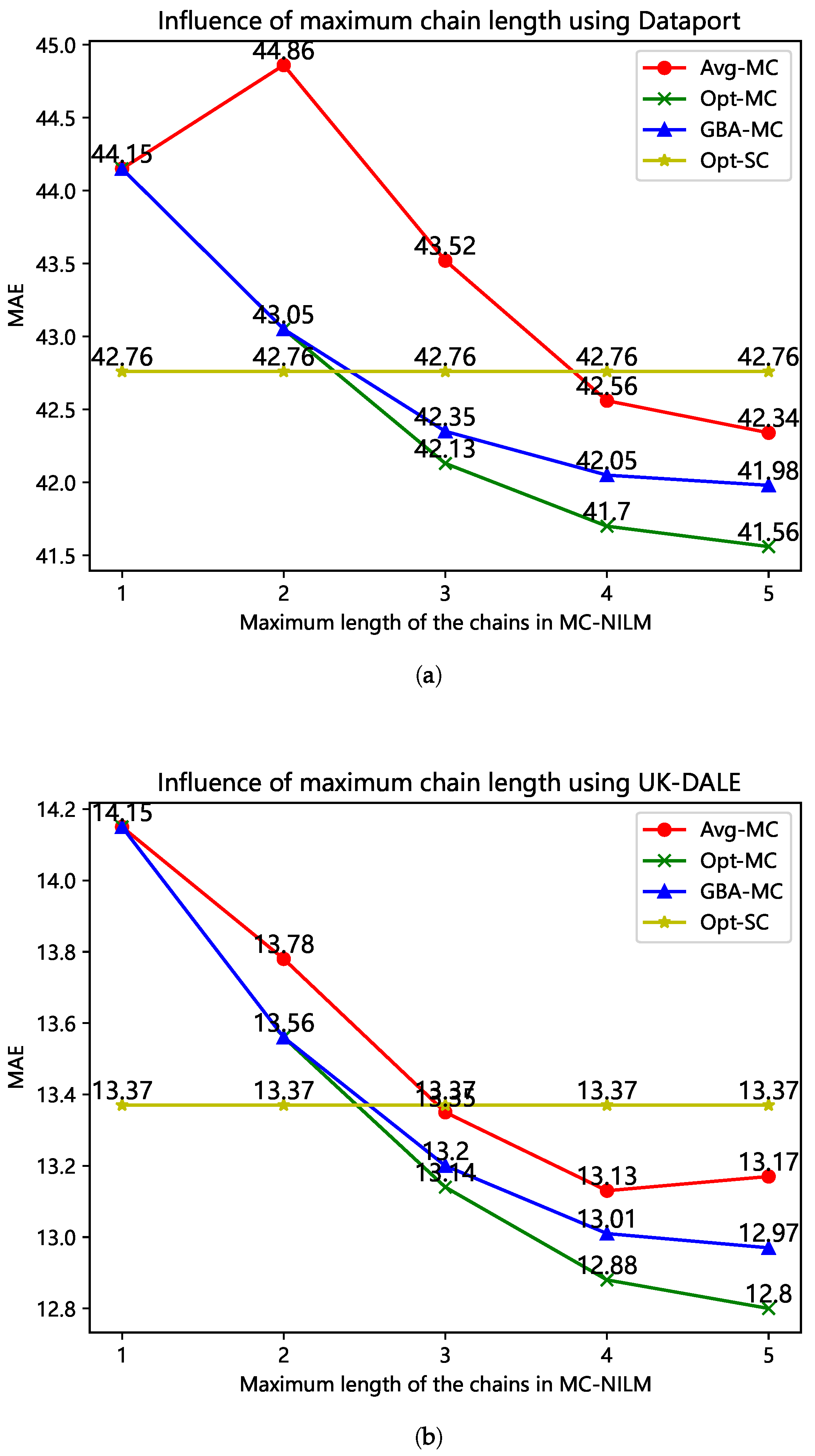
We first evaluated the influence of the maximum length of chains on the performance of MC-NILM. In Figure 2, the performance of the optimal MC-NILM using the brute-force method (Opt-MC), the average performance of all MC-NILM (Avg-MC), the performance of the model obtained by GBA (GBA-MC), and the optimal performance of the model obtained through brute-force method of the SC-NILM (Opt-SC) are compared. We used different methods to create sub-models and experimented on different datasets. For Dataport, we used the CNN network architecture proposed in [26], and for UK-DALE, we used the Seq2point method proposed in [21]. The chain length of the Opt-SC is fixed with the number of target appliances. As shown in Figure 2, although the data in Figure 2a,b are different due to the different datasets and the methods of creating sub-models, the two figures show similar information. For a given maximum length of the chains, the performance of GBA-MC is always better than Avg-MC but slightly worse than the Opt-MC. As the maximum length of the chains increases, the performances of Avg-MC, GBA-MC, and Opt-MC have different improvements. In addition, when the length of the chains is short (i.e., less than 3), the performances of all MC-NILM methods are not as good as the Opt-SC. Besides, as the maximum length of the chains increases, the marginal performance improvement of all MC-NILM models all decreases. Obviously, there exists a trade-off between model performance and complexity.
The GBA-MC reduces the time complexity of creating an MC-NILM by reducing the number of sub-models that need to be trained. In the above experiments, we used two methods of brute-force and GBA to obtain MC-NILM with chains of different maximum lengths. We have counted the number of required sub-models for the two methods, as shown in Table 2. It can be seen from this table that the number of sub-models required by the GBA-MC is no more than that of the Opt-MC, and as the maximum length of the chains increases, the GBA-MC saves more sub-models.
4.3.2. MC-NILM vs. SC-NILM
To verify our proposed MC-NILM and GBA feasibility, we used five methods, two sub-model creation methods, two datasets, and three metrics for experiments. The five methods are:
- (1)
- The brute-force method to obtain the optimal SC-NILM (Opt-SC).
- (2)
- The greedy method to obtain the SC-NILM (Gre-SC) [26].
- (3)
- The brute-force method to obtain the optimal MC-NILM (Opt-MC).
- (4)
- Calculate the average performance of all MC-NILM (Ave-MC).
- (5)
- GBA to obtain the MC-NILM (GBA-MC).
Among them, both Opt-SC and Gre-SC use single-chain structure. The difference lies in the method of obtaining the single-chain structure. Opt-MC, Ave-MC, and GBA-MC are multi-chain structures. To obtain better model performance, we set the maximum length of the chains to the total number of appliances, which is 5. The two sub-model creation methods are still the network architecture used in the [21,26]. The two datasets are Dataport and UK-DALE. The three metrics are MAE, SAE, and F1.
Table 3 shows the experimental results. For different datasets and sub-model creation methods, the best overall model is the Opt-MC. The performance of GBA-MC is slightly worse than that of the Opt-MC, but it is always better than the performance of the Opt-SC and the performance of the Gre-SC. Thus, the MC-NILM scheme outperforms the SC-NILM. It is worth noting that the Avg-MC is sometimes lower than the Opt-SC. In many MC-NILM structures, the sub-models are inappropriate positions, which leads to poor overall performance. Therefore, the careful design of chain structure is necessary.
4.3.3. Generality of MC-NILM
To verify the generality of the MC-NILM, we used a variety of existing NILM methods as sub-models to form an MC-NILM and compare the performance of the original method with the performance of the MC-NILM. In this experiment, we use five methods in NILMTK as sub-models. i.e., edge detection, CO, and Exact FHMM, DAE, and online GRU. We use the UK-DALE dataset and the MAE metric. Since it is time-consuming to obtain the best MC-NILM through the brute-force method, the experiment in this subsection uses GBA to get the MC-NILM with the maximum length of the chain equal to the number of target appliances, which is set to 5. The results in Table 4 show that no matter what underlying model we use as a sub-model, the MC-NILM outperforms the original method. Besides, the framework provides greater performance improvement for deep learning based methods (i.e., DAE and Online GRU) than the other non deep learning based methods (i.e., edge detection, CO and Exact FHMM). The potential reason is that in the process of multi-chain disaggregation, the input of the latter sub-model is the output from the predecessor sub-model. Therefore, the MC-NILM requires the output of sub-models to be as close to the ground truth as possible. The performance of the non deep learning based methods used in this subsection is worse than that of the deep learning based methods, resulting in poor accuracy of the output of the predecessor sub-models, which affects the overall performance of the MC-NILM.
5. Conclusions
Based on the existing independent NILM algorithm for each appliance, this article designs an MC-NILM framework to use these existing models as sub-models to form the overall model. The MC-NILM connects sub-models into different chains for appliances and extracts appliances’ power data from mains iteratively, which improves the overall performance of the energy disaggregation task. When acquiring an MC-NILM, because of the high complexity of obtaining the MC-NILM with the best performance by brute-force methods, two solutions are proposed to solve this problem from a different aspect. The k-length chain method reduces the total number of models generated by the multi-chain scheme by limiting the maximum length of the chain, and we can select a model from all models by brute force or GBA. GBA uses the relative position of each pair of sub-models in a chain for a target appliance to generate multi-chain and only generates one model. The k-length method reduces the time consuming to obtain MC-NILM by adding constraints, while the GBA discovers and uses additional knowledge. The two ways do not conflict and complement each other. The characteristic of k-length methods is that it cannot use the relationship between appliances but is easy to implement, while the GBA method is the opposite. Finally, we conducted experiments on two datasets to verify the feasibility, effectiveness, and generality of the MC-NILM scheme. We will further study better ways to find MC-NILM structures with higher performance and lower complexity in our future work.
Author Contributions
Conceptualization, H.M. and J.J.; methodology, H.M., W.Z. and J.J; software, H.M.; validation, X.Y. and H.Z.; writing—original draft preparation, H.M.; writing—review and editing, J.J., X.Y. and W.Z.; visualization, X.Y.; supervision, J.J.; project administration, J.J.; funding acquisition, W.Z. All authors have read and agreed to the published version of the manuscript.
Funding
This research was funded by China Postdoctoral Science Foundation grant number 2017M611905, Jiangsu Province Graduate Student Cultivation Innovation Project grant number SJCX20_1065, Collaborative Innovation Center of Novel Software Technology and Industrialization and A Project Funded by the Priority Academic Program Development of Jiangsu Higher Education Institutions (PAPD).
Institutional Review Board Statement
Not applicable.
Informed Consent Statement
Not applicable.
Data Availability Statement
The data of Dataport presented in this study are openly available in https://dataport.pecanstreet.org/academic [29]. The data of UK-DALE presented in this study are openly available in https://jack-kelly.com/data/ [30].
Conflicts of Interest
The authors declare no conflict of interest.
References
- Armel, K.C.; Gupta, A.; Shrimali, G.; Albert, A. Is disaggregation the holy grail of energy efficiency? The case of electricity. Energy Policy 2013, 52, 213–234. [Google Scholar] [CrossRef] [Green Version]
- Ridi, A.; Gisler, C.; Hennebert, J. A survey on intrusive load monitoring for appliance recognition. In Proceedings of the 2014 22nd International Conference on Pattern Recognition, Stockholm, Sweden, 24–28 August 2014; pp. 3702–3707. [Google Scholar]
- Ruano, A.; Hernandez, A.; Ureña, J.; Ruano, M.; Garcia, J. NILM techniques for intelligent home energy management and ambient assisted living: A review. Energies 2019, 12, 2203. [Google Scholar] [CrossRef] [Green Version]
- Zhou, B.; Li, W.; Chan, K.W.; Cao, Y.; Kuang, Y.; Liu, X.; Wang, X. Smart home energy management systems: Concept, configurations, and scheduling strategies. Renew. Sustain. Energy Rev. 2016, 61, 30–40. [Google Scholar] [CrossRef]
- Belley, C.; Gaboury, S.; Bouchard, B.; Bouzouane, A. An efficient and inexpensive method for activity recognition within a smart home based on load signatures of appliances. Pervasive Mob. Comput. 2014, 12, 58–78. [Google Scholar] [CrossRef] [Green Version]
- Hart, G.W. Nonintrusive appliance load monitoring. Proc. IEEE 1992, 80, 1870–1891. [Google Scholar] [CrossRef]
- Huber, P.; Calatroni, A.; Rumsch, A.; Paice, A. Review on Deep Neural Networks Applied to Low-Frequency NILM. Energies 2021, 14, 2390. [Google Scholar] [CrossRef]
- Gupta, S.; Reynolds, M.S.; Patel, S.N. ElectriSense: Single-point sensing using EMI for electrical event detection and classification in the home. In Proceedings of the 12th ACM international conference on Ubiquitous Computing, Copenhagen, Denmark, 26–29 September 2010; pp. 139–148. [Google Scholar]
- Tabatabaei, S.M.; Dick, S.; Xu, W. Toward non-intrusive load monitoring via multi-label classification. IEEE Trans. Smart Grid 2016, 8, 26–40. [Google Scholar] [CrossRef]
- Ruzzelli, A.G.; Nicolas, C.; Schoofs, A.; O’Hare, G.M. Real-time recognition and profiling of appliances through a single electricity sensor. In Proceedings of the 2010 7th Annual IEEE Communications Society Conference on Sensor, Mesh and Ad Hoc Communications and Networks (SECON), Boston, MA, USA, 21–25 June 2010; pp. 1–9. [Google Scholar]
- Hassan, T.; Javed, F.; Arshad, N. An empirical investigation of VI trajectory based load signatures for non-intrusive load monitoring. IEEE Trans. Smart Grid 2013, 5, 870–878. [Google Scholar] [CrossRef] [Green Version]
- Figueiredo, M.; Ribeiro, B.; de Almeida, A. Electrical signal source separation via nonnegative tensor factorization using on site measurements in a smart home. IEEE Trans. Instrum. Meas. 2013, 63, 364–373. [Google Scholar] [CrossRef]
- Batra, N.; Dutta, H.; Singh, A. Indic: Improved non-intrusive load monitoring using load division and calibration. In Proceedings of the 2013 12th International Conference on Machine Learning and Applications, Miami, FL, USA, 4–7 December 2013; Volume 1, pp. 79–84. [Google Scholar]
- Kolter, J.Z.; Jaakkola, T. Approximate inference in additive factorial hmms with application to energy disaggregation. In Proceedings of the Machine Learning Research, Volume 22: Artificial Intelligence and Statistics, La Palma, Canary Islands, 21–23 April 2012; pp. 1472–1482. [Google Scholar]
- Lange, H.; Bergés, M. Efficient inference in dual-emission FHMM for energy disaggregation. In Proceedings of the Workshops at the Thirtieth AAAI Conference on Artificial Intelligence, Phoenix, AZ, USA, 12–13 February 2016. [Google Scholar]
- Altrabalsi, H.; Liao, J.; Stankovic, L.; Stankovic, V. A low-complexity energy disaggregation method: Performance and robustness. In Proceedings of the 2014 IEEE Symposium on Computational Intelligence Applications in Smart Grid (CIASG), Orlando, FL, USA, 9–12 December 2014; pp. 1–8. [Google Scholar]
- Zhao, B.; Stankovic, L.; Stankovic, V. On a training-less solution for non-intrusive appliance load monitoring using graph signal processing. IEEE Access 2016, 4, 1784–1799. [Google Scholar] [CrossRef] [Green Version]
- Kelly, J.; Knottenbelt, W. Neural nilm: Deep neural networks applied to energy disaggregation. In Proceedings of the 2nd ACM International Conference on Embedded Systems for Energy-Efficient Built Environments, Seoul, Korea, 4–5 November 2015; pp. 55–64. [Google Scholar]
- do Nascimento, P.P.M. Applications of Deep Learning Techniques on NILM. Master’s Dissertation, Universidade Federal do Rio de Janeiro, Rio de Janeiro, Brazil, 2016. [Google Scholar]
- Kim, J.; Kim, H.; Le, T.-T.-H. Classification performance using gated recurrent unit recurrent neural network on energy disaggregation. In Proceedings of the 2016 international conference on machine learning and cybernetics (ICMLC), Jeju, Korea, 10–13 July 2016; Volume 1, pp. 105–110. [Google Scholar]
- Zhang, C.; Zhong, M.; Wang, Z.; Goddard, N.H.; Sutton, C.A. Sequence-to-Point Learning with Neural Networks for Non-Intrusive Load Monitoring; AAAI: Menlo Park, CA, USA, 2018. [Google Scholar]
- Pan, Y.; Liu, K.; Shen, Z.; Cai, X.; Jia, Z. Sequence-to-subsequence learning with conditional gan for power disaggregation. In Proceedings of the ICASSP 2020-2020 IEEE International Conference on Acoustics, Speech and Signal Processing (ICASSP), Barcelona, Spain, 4–8 May 2020; pp. 3202–3206. [Google Scholar]
- Puente, C.; Palacios, R.; González-Arechavala, Y.; Sánchez-Úbeda, E.F. Non-Intrusive Load Monitoring (NILM) for Energy Disaggregation Using Soft Computing Techniques. Energies 2020, 13, 3117. [Google Scholar] [CrossRef]
- Piccialli, V.; Sudoso, A.M. Improving Non-Intrusive Load Disaggregation through an Attention-Based Deep Neural Network. Energies 2021, 14, 847. [Google Scholar] [CrossRef]
- Lee, J.; Yoon, S.; Hwang, E. Frequency Selective Auto-Encoder for Smart Meter Data Compression. Sensors 2021, 21, 1521. [Google Scholar] [CrossRef]
- Jia, Y.; Batra, N.; Wang, H.; Whitehouse, K. A tree-structured neural network model for household energy breakdown. World Wide Web Conf. 2019, 2872–2878. [Google Scholar] [CrossRef]
- Batra, N.; Kelly, J.; Parson, O.; Dutta, H.; Knottenbelt, W.; Rogers, A.; Singh, A.; Srivastava, M. NILMTK: An open source toolkit for non-intrusive load monitoring. In Proceedings of the 5th International Conference on Future Energy Systems, Cambridge, UK, 11–13 June 2014; pp. 265–276. [Google Scholar]
- Sadeghianpourhamami, N.; Ruyssinck, J.; Deschrijver, D.; Dhaene, T.; Develder, C. Comprehensive feature selection for appliance classification in NILM. Energy Build. 2017, 151, 98–106. [Google Scholar] [CrossRef] [Green Version]
- Parson, O.; Fisher, G.; Hersey, A.; Batra, N.; Kelly, J.; Singh, A.; Knottenbelt, W.; Rogers, A. Dataport and NILMTK: A building data set designed for non-intrusive load monitoring. In Proceedings of the 2015 IEEE Global Conference on Signal and Information Processing (Globalsip), Orlando, FL, USA, 14–16 December 2015; pp. 210–214. [Google Scholar]
- Kelly, J.; Knottenbelt, W. The UK-DALE dataset, domestic appliance-level electricity demand and whole-house demand from five UK homes. Sci. Data 2015, 2, 1–14. [Google Scholar] [CrossRef] [PubMed] [Green Version]
- Hart, G.W. Prototype Nonintrusive Appliance Load Monitor: Progress Report 2; MIT Energy Laboratory: Cambridge, MA, USA, 1985. [Google Scholar]
- Batra, N.; Singh, A.; Whitehouse, K. If you measure it, can you improve it? exploring the value of energy disaggregation. In Proceedings of the 2nd ACM International Conference on Embedded Systems for Energy-Efficient Built Environments, Seoul, Korea, 4–5 November 2015; pp. 191–200. [Google Scholar]
- Parson, O.; Ghosh, S.; Weal, M.; Rogers, A. Non-intrusive load monitoring using prior models of general appliance types. In Proceedings of the Twenty-Sixth AAAI Conference on Artificial Intelligence, Toronto, ON, Canada, 22–26 July 2012; pp. 356–362. [Google Scholar]
- Krystalakos, O.; Nalmpantis, C.; Vrakas, D. Sliding window approach for online energy disaggregation using artificial neural networks. In Proceedings of the 10th Hellenic Conference on Artificial Intelligence, Patras, Greece, 9–12 July 2018; pp. 1–6. [Google Scholar]
Figure 1.
Schematic diagram of three energy disaggregation methods. (a) Independent method; (b) SC-NILM; (c) MC-NILM. (AC: Air conditioner, FR: Fridge freezer, WD: Wash dryer, DW: Dish washer, MW: Microwave).
Figure 1.
Schematic diagram of three energy disaggregation methods. (a) Independent method; (b) SC-NILM; (c) MC-NILM. (AC: Air conditioner, FR: Fridge freezer, WD: Wash dryer, DW: Dish washer, MW: Microwave).

Figure 2.
The influence of the maximum chain length on the performance of the MC-NILM. (a) Results of experiments using the Dataport; (b) Results of experiments using the UK-DALE.
Figure 2.
The influence of the maximum chain length on the performance of the MC-NILM. (a) Results of experiments using the Dataport; (b) Results of experiments using the UK-DALE.


Table 1.
Power-on threshold for each appliance.
| Appliance | Kettle | Microwave | Dish Washer | Fridge Freezer | Wash Dryer | Air Conditioner |
|---|---|---|---|---|---|---|
| Threshold | 2000 | 200 | 10 | 50 | 20 | 1000 |
Table 2.
Numbers of sub-models required for the the Opt-MC and GBA-MC.
| Max Length | 1 | 2 | 3 | 4 | 5 |
|---|---|---|---|---|---|
| Opt-MC | 5 | 25 | 55 | 75 | 80 |
| GBA-MC | 5 | 25 | 30 | 34 | 37 |
Table 3.
Performance of different methods on different datasets.
| Dataset | Metrics | Opt-SC | Gre-SC | Ave-MC | Opt-MC | GBA-MC |
|---|---|---|---|---|---|---|
| Dataport | MAE | 42.763 | 43.819 | 42.359 | 41.561 | 41.982 |
| SAE | 0.402 | 0.426 | 0.356 | 0.310 | 0.326 | |
| F1 | 0.424 | 0.402 | 0.459 | 0.497 | 0.462 | |
| UK-DALE | MAE | 13.372 | 13.938 | 13.171 | 12.801 | 12.972 |
| SAE | 0.112 | 0.125 | 0.114 | 0.090 | 0.099 | |
| F1 | 0.563 | 0.538 | 0.581 | 0.633 | 0.620 |
Table 4.
Improvements of GBA-NILM over the original model in terms of the MAE metric.
| Method | Edge Detection | CO | Exact FHMM | DAE | Online GRU |
|---|---|---|---|---|---|
| Original method | 68.673 | 61.379 | 53.744 | 18.423 | 11.469 |
| GBA-NILM | 65.903 | 57.800 | 49.909 | 16.902 | 10.389 |
| Improvement (%) | 4.034 | 5.831 | 7.136 | 8.256 | 9.417 |
Publisher’s Note: MDPI stays neutral with regard to jurisdictional claims in published maps and institutional affiliations. |
© 2021 by the authors. Licensee MDPI, Basel, Switzerland. This article is an open access article distributed under the terms and conditions of the Creative Commons Attribution (CC BY) license (https://creativecommons.org/licenses/by/4.0/).
Share and Cite
MDPI and ACS Style
Ma, H.; Jia, J.; Yang, X.; Zhu, W.; Zhang, H. MC-NILM: A Multi-Chain Disaggregation Method for NILM. Energies 2021, 14, 4331. https://doi.org/10.3390/en14144331
AMA Style
Ma H, Jia J, Yang X, Zhu W, Zhang H. MC-NILM: A Multi-Chain Disaggregation Method for NILM. Energies. 2021; 14(14):4331. https://doi.org/10.3390/en14144331
Chicago/Turabian StyleMa, Hao, Juncheng Jia, Xinhao Yang, Weipeng Zhu, and Hong Zhang. 2021. "MC-NILM: A Multi-Chain Disaggregation Method for NILM" Energies 14, no. 14: 4331. https://doi.org/10.3390/en14144331
Note that from the first issue of 2016, this journal uses article numbers instead of page numbers. See further details here.