Economic and Environmental Assessment on Implementing Solar Renewable Energy Systems in Spanish Residential Homes

Abstract

In Europe, buildings are responsible for more than one third of the total final energy demands and greenhouse gas emissions. In the last twenty years, the European Union has published a succession of energy performance of building directives to define and ensure the fulfilment of a series of objectives regarding greenhouse gas emissions, energy consumption, energy efficiency and energy generation from renewable sources in buildings. For its part, Spain is adapting its legal framework, transposing these directives with the aim of achieving greater energy efficiency and sustainability for buildings. Under this context, an energy, economic and environmental assessment is performed to analyze the impact of these regulatory changes on a single-family home including a photovoltaic installation for self-consumption with surpluses and/or a solar thermal installation for domestic hot water supply, located in each one of the eight thousand one hundred thirty-one municipalities that make up Spain. The energy behavior of the original house is compared with that obtained after it is updated with these new facilities. The transient system simulation tool is used for the energy study. The results show that the European objectives are far exceeded. The energy savings achieved range from 67% to 126%, carbon dioxide emissions decrease by 42% to 100% and energy bills are reduced in cost by 32% to 81%. The findings of this work can be used by policymakers as guidelines for the development of national strategic plans and financial incentives for the promotion of small-scale residential photovoltaic and solar thermal applications, as well as by designers, supervisors, managers and developers to include them in their projects.

1. Introduction

Buildings have become the largest energy consumers in Europe, accounting for approximately 40% of European Union (EU) energy consumption and 36% of greenhouse gas (GHG) emissions [1]. In this context, buildings must face the challenge of achieving energy management that enables them to contribute to economic growth, social welfare and sustainability, while preserving non-renewable resources and the natural environment [2]. In addition, they have the opportunity of adopting measures aimed at saving energy, reducing their demand and/or improving the efficiency of their systems [3]. Among them, the EU residential building stock offers high potential for energy efficiency gains and reduction of GHG emissions [4]. This is due to the heavy reliance on fossil fuels in household activities, to cover the demand for heating and domestic hot water (DHW) [5], as well as to a lesser extent and indirectly for cooling, lighting and appliances. However, occupant behavior lifestyles cannot be underrated [6], although this issue is outside the scope of this research.

The use of renewable energy systems (specifically those based on solar ones) may be a solution to reduce the GHG emissions from residential buildings, as well as save money on energy bills. Therefore, the objective of this study is to assess the triple energy (in consumption), economic (in savings and/or surplus) and environmental (in GHG emissions) impact that the incorporation of a photovoltaic (PV) and/or a solar thermal (ST) system produces in the use phase of a single-family house. This study will be extended to the entire territory of Spain, analyzing all its municipalities.

Looking for zero energy and emissions future, European legal framework has become more and more strict over the years. In this regard, the Energy Performance of Building Directives (EPBDs) aim to ensure compliance with EU objectives related to energy consumption, GHG emissions and energy efficiency. This includes the energy generation from renewable sources in buildings.

The first version of the EPBD 2002/91/EC [7] provided energy use requirements for both new and existing buildings under renovation and introduced energy performance certificates. Next, the EPBD 2010/31/EU [8] specified that by the end of 2020, all new buildings should be nearly Zero-Energy Buildings (nZEBs). Then, the EPBD 2012/27EU [9] imposed a mandatory requirement for Member States to develop national plans to increase the number of nZEBs, which should include a detailed definition of the concept of a nZEB considering their national, regional and/or local conditions, as well as a numerical indicator of primary energy use. Finally, the EPBD 2018/844/EU [10] modified the two prior directives, stressing the EU’s engagement in the fight against climate change and energy poverty. To do this, the EU has set as primary objectives to:

• Decarbonize the housing stock, renovating it from an energy standpoint.
• Ensure equal access to financing for building renovation, rewarding proposals that promote energy efficiency.
• Guarantee the quality of buildings, prioritizing the adoption of natural solutions, the encouragement of alternative high-efficiency installations, the promotion of research and the test of new solutions.

According to the EPBDs, Member States have to promote the improvement of the energy performance of buildings within their territories, taking into account outdoor climatic conditions, indoor climate requirements and cost-effectiveness [10]. The goal is to reduce GHG emissions in the Union by 80–95% compared to 1990, to ensure a highly energy efficient and decarbonized European building stock and to facilitate the cost-effective transformation of existing buildings into nZEBs.

In short, EPBDs set EU building sustainability objectives for mitigating climate change, reducing GHG emissions and energy consumption and promulgating the contribution of renewable energy. By 2020, the EU has set the target to reduce GHG emissions and energy consumption by 20%, as well as to raise the share of renewable energy in their energy consumption by a further 20%, compared to 1990 results. By 2030, the EU has established a 40% reduction in GHG emissions and a 32.5% in energy consumption, as well as a 32% contribution from renewable energy sources.

In Spain, many standards, regulations and laws have been published this century, with the aim of achieving greater energy efficiency and sustainability for buildings. The Spanish Building Act (LOE) 38/1999 [11] required the adoption of a Technical Building Code (CTE), which came into force in 2008 by the Royal Decree (RD) 384/2006 [12]. This transposed the EPBD 2002/91/EC, definitively repealing the Basic Building Standard on Thermal Conditions in buildings (NBE CT-79) [13]. After that, a few RDs (1371/2007, 238/2013) and Ministerial Orders (VIV/984/2009, FOM/1635/2013, FOM/588/2017) transposed the 2010/31/EU and 2012/27EU EPBDs, focusing on the processing of energy certifications, the regulation of thermal installations, the updating of energy demands and the limitation of energy consumption. Finally, the RD 732/2019 [14] once again modified the CTE, increasing the conditions to control the energy demand and limiting the energy consumption. This last version incorporated the considerations of the 2018/844/EU EPBD, with the purpose of reducing the energy required to satisfy the energy demand associated with the use of buildings, eventually incorporating the definition of nZEB for Spain. Furthermore, in the same year, the RD 244/2019 [15] regulated the conditions for self-consumption of electricity. This eliminated the so-called “sun tax” and even allowed the sale of surplus from small-scale producers for generation plants of less than 100 kWp.

The EU has assumed the leading role in achieving the goals of substitution of fossil fuels with renewable energy sources, reduction of GHG emissions and other environmental impacts [16]. The share of renewable energy sources on the gross final energy consumption has grown up from 11% in 2005 to 19.5% in 2017 [17], although the achievement of these objectives has been quite heterogeneous. In this context, the case of Spain must be highlighted, since the share of electricity production from renewables reached 43.66% in 2020 [18]. In addition, carbon dioxide equivalent (CO₂eq) emission-free production accounted for 66.9% of total generated, becoming the cleanest year registered.

The PV market for electricity generation has developed strongly in the recent years (102.4 GWp of grid-connected PV panels were installed globally in 2018, which is equivalent to the total PV capacity available in the world in 2012 (100.9 GWp)), leading to a total global solar power capacity of more than 500 GWp at the end of 2018 [16]. Regarding ST systems, the global ST market size stood at 496.15 GWp in 2018 and is projected to reach 767.73 GWp by 2026, exhibiting a compound annual growth rate of 5.6% during the forecast period [19].

Although the potential of renewable energy sources in buildings is under study from different points of view (as efficiency [20], employment [21], market [22] or sustainability [23], for example), the scientific community is paying special attention to the performance assessment of different renewable energy sources (hydrogen, PV, ST, wind, etc.) with a life cycle approach [16,24,25,26,27,28]. Some of them include an energy study of the use of renewable energy sources [17,29]. Others include both an economic and an environmental analysis to determine the payback period [30,31]. Some others include, instead, the evaluation of the energy profile of different renewable energy technologies [32,33].

At present, there are few new buildings in construction in Spain, but a large number are 10–20 years old, with a long useful life remaining (at least 30 years more [34]). In addition, most of these buildings (both existing and new ones) are residential homes. This leads to the need to focus on solving the renovation of existing buildings rather than promoting the development of new ones [35,36,37,38]. However, most of the current studies are aimed either at analyzing a case study (in a particular location [39,40], of a determined typology [41,42], with a specific technology [43,44], etc.) or at analyzing future developments that are not yet available on the market for the public [45,46].

As stated at the beginning of this section, the objective of this study is to assess the energy, economic and environmental impact that the incorporation of a PV and/or a ST system produces in a new or existing single-family home with at least 30 years of useful life remaining. Present-day conditions (mounting requirements, operation and maintenance instructions, technical performance, product warranty, etc.) from current commercial solutions are assumed. The analysis is carried out with satellite climatic data from the European Photovoltaic Geographical Information System (PVGIS) [47] from the last typical meteorological year (TMY) available, calculated from the period 2007–2016. This evaluation has been carried out by means of energy simulation for each of the 8131 municipalities of Spain (including mainland Spain, the Canary and Balearic Islands and the autonomous cities of Ceuta and Melilla in Africa). Some of the contributions of the paper can be summarized as follows:

• Two scenarios will be studied for each system. In the case of the PV system, all energy generated is consumed at home or sold to the supplier company and, for the ST system, auxiliary energy is supplied by electricity or natural gas.
• Forecast scenarios proposed by the EU both for the electricity and natural gas prices and for the energetic mix will be considered.
• Usual energy, economy, and emissions indicators of the considered solar systems (PV, ST) will be accomplished.
• Initial, operational and maintenance costs and GHG emissions incurred by PV and ST systems will be compared to the costs and GHG emissions from fossil-fuel-based systems to which they replace and/or complement.
• The amount of money and CO₂eq that can be saved when a household is using either a PV and/or a ST system to support the energy consumption will be quantified.
• Energy, money, and CO₂eq emissions saving maps will be generated for the different scenarios considered.

This way, the relevance of these measures for an entire country can be checked, the influence of the climatic conditions of each territory on its different energy needs can be considered and various existing technologies can be compared from different points of view. Accordingly, the findings of this study can help construction professionals (such as designers, architects and engineers, developers, builders and even legislators) to quantify the real impact that domestic solar renewable energy systems may have on energy, economic and emissions savings.

The rest of the paper is organized as follows: Section 2 describes the material and methods used for the calculation of the variables selected (energy, costs and GHG emissions): climate data, characterization of renewable energy facilities, economic and environmental study of the solar renewable energy facilities, energy simulation, energy, economic and emissions assessment and geographic information system (GIS) representation. Then, the results are presented in Section 3. Next, the energy, economic and environmental performance of the systems analyzed (conventional, PV and ST) are discussed. Finally, in Section 5, some conclusions and recommendations are highlighted.

2. Materials and Methods

To quantify the impact of incorporating solar renewable energy systems in the transformation of existing and new single-family homes into nZEBs, the energy behavior, energy costs and GHG emissions of a house without renewable energy sources has been compared to a house that incorporates them. This comparison has been made considering four premises:

S1.

House in which a PV system has been added under the assumption that the entire production will be used for self-consumption (PV consumption saving scenario).

S2.

House in which a PV system has been added under the assumption that the entire production will be sold (PV surplus sale scenario).

S3.

House in which a ST system has been added to a previous DHW one with an electric boiler, that remains as an auxiliary energy system (ST auxiliary electricity scenario).

S4.

House in which a ST system has been added to a previous DHW one supplied by natural gas, that remains as an auxiliary energy system (ST auxiliary natural gas scenario).

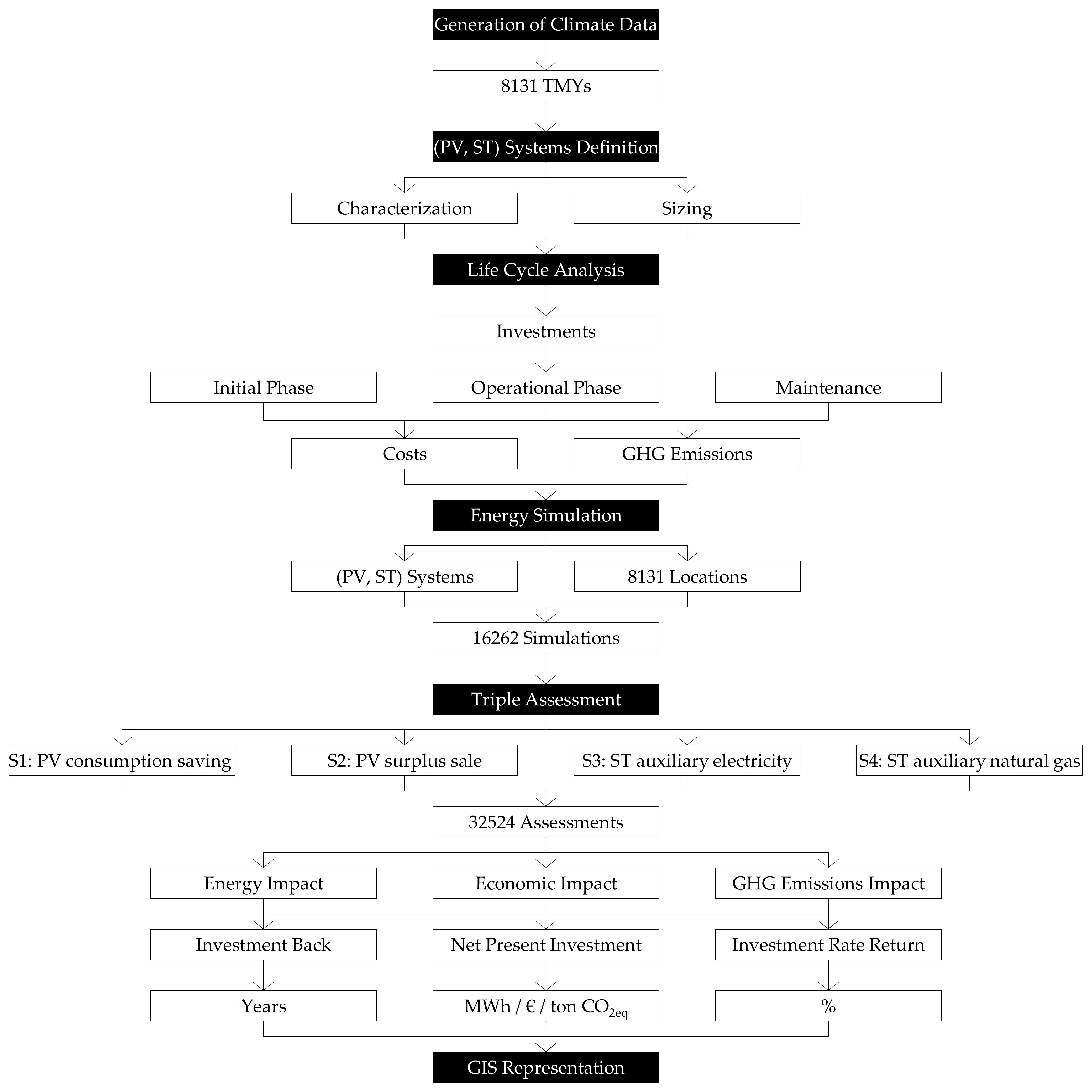
Once the scenarios are defined, a sequential method to approach the problem is established. To culminate this comparative study, the following steps need to be undertaken, as summarized in Figure 1:

• Generation of climate data for each municipality, provided by PVGIS depending on its latitude and longitude.
• Characterization and sizing of solar renewable energy facilities incorporated (PV and/or ST). This configuration remains for each location, considering their local climate data.
• Economic and environmental study of the solar renewable energy facilities included (PV, ST).
• Energy simulation for the 16,262 combinations (2 solar renewable energy installations (PV, ST), 8131 municipalities).
• Energy, economic and GHG emissions assessment of the 32,524 case studies (2 scenarios for each of the 2 solar renewable energy systems (PV, ST) in the 8131 municipalities).
• Representation of the evaluated data by means of a GIS software. These will show the average energy consumption, carbon dioxide emissions and energy costs over the 30 years of life, considering the initial emissions and investments and the corresponding performance losses, according to each assumption.

Figure 1. Research methodology scheme.

Figure 1. Research methodology scheme.

2.1. Climate Data

The PVGIS database is a project developed in 2001 by the publicly accessible European Commission Joint Research Centre, designed to allow the users to calculate photovoltaic production anywhere in Europe, among others. From the application, monthly, daily, or hourly weather data can be generated, as well as a TMY for each coordinate (by longitude and latitude) entered.

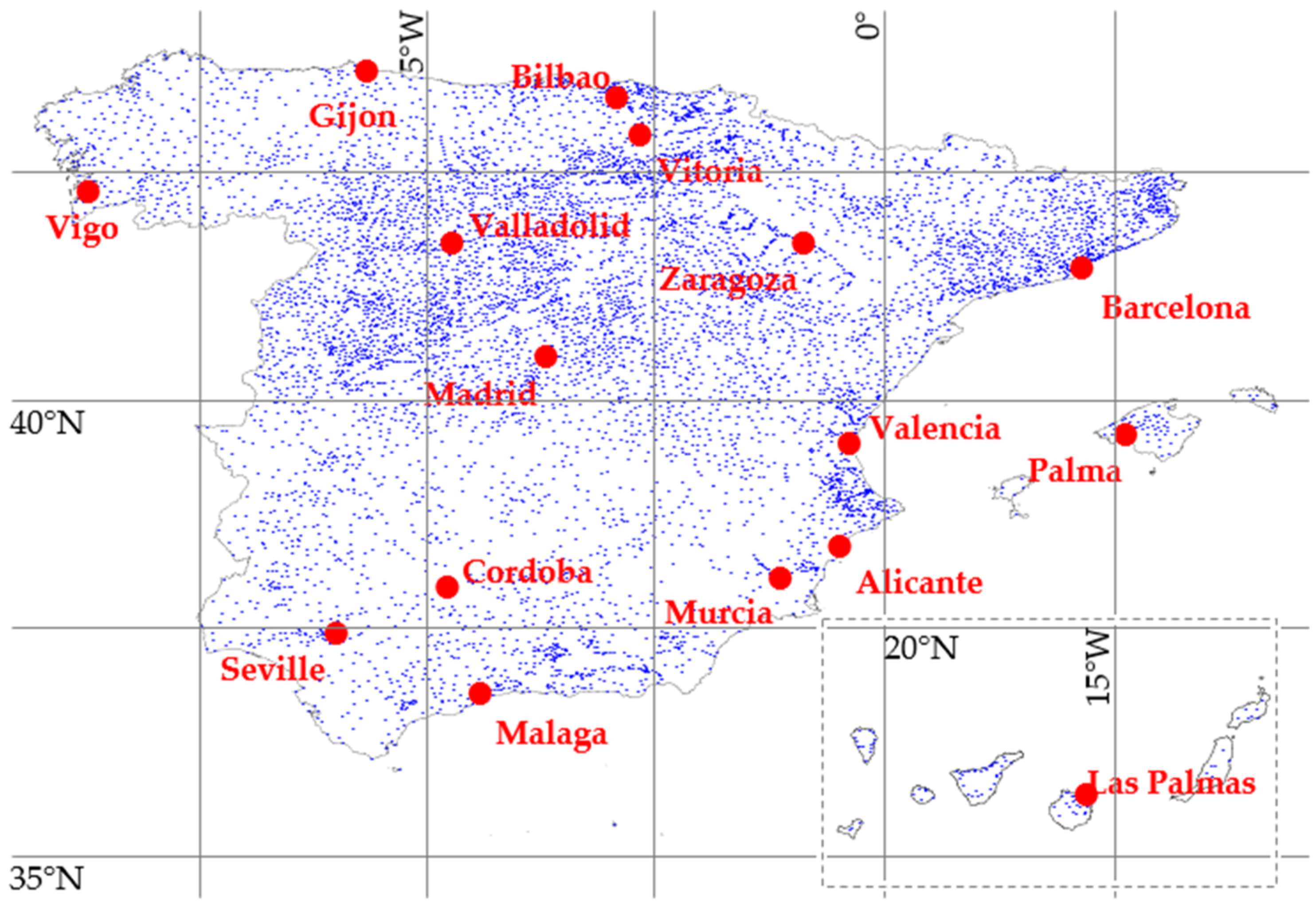
The PVGIS obtains this data by interpolation [48], based on solar radiation data obtained by satellite, solar irradiation measured in Europe’s network of weather stations, turbidity and digital elevation, providing all the climate values necessary for the generation of a TMY [49]. This study has compiled the 8131 TMYs for the period 2007–2016 (the most recent available data) corresponding to the geographical location of each municipality in Spain (in blue), as shown in Figure 2. For the sake of clarity, the sixteen cities with a population of more than a quarter of a million inhabitants will be also highlighted (in red).

2.2. Characterization of Renewable Energy Facilities

Two solar renewable energy systems have been selected for the study. On the one hand, a PV system of 2.4 kWp using 6 monocrystalline cell modules (with a nominal power rating of 400 Wp per unit) has been installed. The modules have a surface area of 2 square meters, a nominal operating cell temperature (NOCT) of 47 °C, and a temperature degradation coefficient of 0.36%/°C. It can be noted that this type of renewable energy source is not mandatory in Spain for residential buildings, even in the last version of the CTE. However, from the entry into force of the Royal Decree 244/2019, the surplus produced by a household system can be fed into the electric grid (if the facility is lower than 100 kWp), making the entire production available for use.

On the other hand, a ST system is pre-dimensioned so that approximately 80% of the demand for DHW is covered (slightly above the legal minimum of 70%), using a 10-pipe evacuated tube collector. It has a surface area of 2 square meters, an optical efficiency of 93% and an overall loss coefficient of 1.06 W/m²/K. This type of renewable energy source partially covering the demand for DHW is mandatory since the regulatory framework of the first CTE, for all new buildings or renovation of existing ones. A DHW flow rate of 140 L/d (5 occupants at a rate of 28 L/d per person) is considered, so an accumulation volume of 200 L will be used.

2.3. Economic and Environmental Study of the Solar Renewable Energy Facilities

The incorporation of the solar renewable energy facilities (the PV system that is optional for residential buildings of any type according to CTE and the ST one, which is mandatory according to the CTE for both renovation and new buildings) generates an environmental impact and supposes an initial economic investment, the return on which must be calculated. The economic evaluation of the PV system involves comparing its initial, operational and maintenance costs with the energy costs of the electricity consumption that is no longer consumed (S1: PV saving scenario) or of the sale of the surplus produced (S2: PV surplus sale scenario). In the case of the ST system, the economic evaluation consists of comparing its initial, operational and maintenance costs with the savings from the consumption of auxiliary energy, either electricity (S3) or natural gas (S4).

The energy prices considered to be saved (or sold) come from the two major supply companies in Spain (Endesa [50] and Iberdrola [51] for electricity and Naturgy [52] and Repsol [53] for natural gas). These prices are summarized in

Table 1. Electricity price (in €).

Electric Consumption		Price	Electric Taxes	VAT	Total Price
[54]	Eurostat 2018 S1	0.1874	0.0096	0.0414	0.2383
	Eurostat 2019 S1	0.1889	0.0097	0.0417	0.2403
	Eurostat 2020 S1	0.1760	0.0090	0.0389	0.2239
[55]	Power Choices Reloaded 2050	0.1910	0.0098	0.0422	0.2429
[50]	Endesa 10 Peak (18 h)	0.1546
	Endesa 10 Off-Peak (6 h)	0.1159
	Endesa 10 Mean	0.1449	0.0074	0.03199	0.1843
[51]	Iberdrola 10 Peak (16 h)	0.1811
	Iberdrola 10 Off-Peak (8 h)	0.0889
	Iberdrola 10 Mean	0.1504	0.0077	0.03319	0.1912
Price considered		0.1476	0.0075	0.03259	0.1878
Electric surplus sale		Price	Electric taxes	VAT	Total price
[50]	Endesa 10	0.0500	0.0026	0.01104	0.0636
[51]	Iberdrola 10	0.0510	0.0026	0.01126	0.0649
Price considered		0.0505	0.0026	0.01115	0.0642

and

Table 2. Natural gas price (in €).

Natural Gas Consumption		Price	Hydrocarbon Taxes	VAT	Total Price
[54]	Eurostat 2018 S1	0.0665	0.0002	0.01400	0.0807
	Eurostat 2019 S1	0.0736	0.0002	0.01549	0.0893
	Eurostat 2020 S1	0.0718	0.0002	0.01511	0.0871
[55]	Power Choices Reloaded 2050	0.0658	0.0002	0.01385	0.0799
[52]	Naturgy	0.0588	0.0001	0.01238	0.0713
[53]	Repsol	0.0599	0.0001	0.01261	0.0726
Price considered		0.0594	0.0001	0.01249	0.0720

. It can be noted that all the prices selected are lower than those from the Statistical Office of the European Union (Eurostat) [54], as well as lower than the expected future scenarios in the EU up to 2050 forecasted by the Union of the Electricity Industry (Eureletric) [55]. In this study, E³Mlab proposes 8 different scenarios (according to the magnitude of change that the delay or failure of specific elements cause): reference, power choices reloaded, lost decade 2020–2030, limited financing, RES target in 2030, limited XB trade, barriers to EE and CO₂ price driven. As the lowest price predicted for any of the eight scenarios from 2020 to 2050 is higher than the average price obtained from the supply companies, it is decided to leave the latter price as constant, so the study is on the reliable side.

For the cost definition of the elements that compose both systems, the price database from CYPE Engineers’ Archimedes software, version 2021.f [56] is used, facilitating their traceability. For this purpose, a Spanish national manufacturer has been chosen, whose production and distribution facilities are located in the city of Valencia. In economic terms, unit prices include the waste management, health and safety, overheads, industrial profits, technical fees, municipal licenses and indirect taxes. These initial costs, as well as operational and maintenance costs, are also summarized in

Table 3. Initial costs from PV system.

Element		Amount	Unit Price	Cost
[56]	Panel	6	175.00	1050.00
	Inverter (15 years)	1	409.10	409.10
	Charge Regulator	1	140.45	140.45
	Structural Base	6	30.00	180.00
	Bidirectional Counter	1	140.45	140.45
	Protection Panel	1	180.00	180.00
Assembly and Legalization		1	400.00	200.00
Budget				2600.00
VAT (10%)				260.00
Tender				2860.00

Prices (in €) referring to the CYPE Arquimedes 2021.f database [56].

,

Table 4. Maintenance costs from PV system.

Element		Amount	Unit Price	Cost
[56]	Inverter (every 15 years)	1	409.10	409.10
VAT (21%)				85.90
Tender				495.00

Prices (in €) referring to the CYPE Arquimedes 2021.f database [56].

,

Table 5. Initial costs from ST system.

Element		Amount	Unit Price	Cost
[56]	Vacuum-Tube Collector (10 tubes)	2	830.00	1660.00
	Hot Water Cylinder (200 L)	1	570.00	570.00
	Expansion Vessel	1	150.00	150.00
	Structural Base	2	30.00	60.00
	Circulator Pump	1	360.00	360.00
Assembly and Legalization		1	400.00	200.00
Budget				3200.00
VAT (10%)				320.00
Tender				3520.00

Prices (in €) referring to the CYPE Arquimedes 2021.f database [56].

,

Table 6. Operational costs from ST system.

Element		Amount	Unit Price	Cost
**	Pumping Electricity (kWh/year)	(30 × 48) 1440	0.1552	223.48
VAT (21%)				46.92
Tender				270.40

Prices (in €) referring to the CYPE Arquimedes 2021.f database [56]. ** Price from Table 1.

and

Table 7. Maintenance costs from ST system.

Element		Amount	Unit Price	Cost
[56]	Heat Transfer Fluid (every 5 years)	(5 × 2) 10	13.64	136.36
VAT (21%)				28.64
Tender				165.00

Prices (in €) referring to the CYPE Arquimedes 2021.f database [56].

, for each of the facilities considered. However, no inflation or deflation rates have been considered for those costs to be paid in the operation and maintenance phase, due to the small relative amount (9% of total investment) and the uncertainty after the COVID-19 pandemics [57].

In terms of environmental impact, a life cycle inventory of all the elements needed to incorporate the PV and ST facilities has been made. For the PV system, the FU is composed by 6 monocrystalline cell modules (described previously) with their structural base, a charge regulator, a bidirectional counter and a protection panel. For the ST system, the FU is composed by a 10-pipe evacuated tube collector (described previously) with its structural base, a hot water cylinder (200 L), an expansion vessel and a circulator pump. For the analysis, the following stages of the life cycle of both systems have been considered: manufacture, transport of systems to the final locations, installation and operation. This includes the transportation of materials to the factory, energy required for production and logistics distribution. The manufacturing site is located in Valencia (Spain). As well, decommissioning of systems has not been included.

The conversion factors to obtain CO₂eq emissions are then determined using EcoInvent 3.3 database [58] and the Intergovernmental Panel on Climate Change (IPCC) 2013 method with a timeframe of 100 years [59]. As a result, CO₂eq emissions from these interventions for the FU are shown in

Table 8. (a) Manufacture emissions from PV system. (b) Manufacture emissions from PV system.

Element	Component	Material	Amount	CF	Emissions
(a)
PV Modules (6 units, 12 m2)	Cells	Photovoltaic cell, single-Si (m2)	10.89	251.00	2732.83
	Materials	Aluminum alloy, AlMg3 (kg)	25.56	9.43	241.03
		Tin (kg)	0.15	21.50	3.33
		Lead (kg)	0.01	2.37	0.02
		Diode (kg)	0.03	295.00	9.95
		Polyethylene, HDPE (kg)	0.29	2.09	0.60
		Solar glass, low-iron (kg)	105.72	1.13	119.46
		Copper (kg)	1.24	7.82	9.67
		GFRP, polyamide, injection molded (kg)	3.54	9.14	32.36
		Ethylvinylacetate, foil (kg)	10.50	2.97	31.19
		Polyvinylfluoride film (kg)	1.34	20.90	28.09
		PET, granulate, amorphous (kg)	4.15	2.98	12.37
		Silicone product (kg)	1.46	3.18	4.66
	Auxiliary materials	Corrugated board, mixed fiber, single wall (kg)	9.16	1.08	9.98
		1-propanol (kg)	0.19	4.51	0.86
		EUR-flat pallet (unit)	0.05	8.88	0.44
		Hydrogen fluoride (kg)	0.75	3.52	2.64
		Isopropanol (kg)	0.00	1.85	0.00
		Potassium hydroxide (kg)	0.62	2.14	1.32
		Soap (kg)	0.14	6.31	0.88
	Technosphere	Electricity, medium voltage, production ENTSO (kWh)	44.76	0.46	20.46
		Diesel, burned in building machine (kg)	0.00	0.55	0.00
	Infrastructure	Tap water (kg)	60.36	0.00	0.02
		Tempering, flat glass (kg)	105.72	0.17	17.87
		Wire drawing, copper (kg)	1.24	0.76	0.94
Element	Component	Material	Amount	CF	Emissions
(b)
Structure	Technosphere	Aluminum (kg)	030.24	009.43	285.16
		Corrugated board (kg)	000.22	001.08	000.24
		Polyethylene, high density, HDPE (kg)	023.04	002.09	048.15
		Polystyrene, high impact, HIPS (kg)	000.10	003.72	000.37
		Steel, low-alloyed (kg)	003.20	001.90	006.09
	Materials	Copper (kg)	001.00	007.82	007.85
		TPE = Thermoplastic elastomere (kg)	000.79	004.91	003.89
Inverter 2.5 kW (15 years)	Materials	Steel (kg)	009.80	001.90	018.62
		Aluminum (kg)	001.40	009.43	013.20
		Transformers, wire-wound (kg)	005.50	005.41	029.76
		Printed Circuit Board, with electronic components (kg)	001.80	247.00	444.60
Charge Regulator	Materials	Steel (kg)	005.11	001.90	009.71
		Aluminum (kg)	000.47	009.43	004.40
		Copper (kg)	001.19	007.82	009.29
		Polyamide injection molded (kg)	000.25	009.14	002.31
		Polyester (kg)	000.16	003.72	000.58
		Polyethylene, HD (kg)	000.08	002.09	000.16
		Paint (kg)	000.08	006.50	000.51
		Printed Circuit Board, with electronic components (kg)	000.31	247.00	077.31
Transport		Components and materials (kg)	416.96	000.04	031.18
Sum					4243.05

Data from EcoInvent 3.3 [58]. CF: conversion factor in kg CO₂eq/kg. Emissions in kg CO₂eq (per FU).

,

Table 9. Maintenance emissions from PV system.

Element	Component	Material	Amount	CF	Emissions
Infrastructure		Tap water (kg)	1810.80	000.00	000.68
Inverter 2.5 kW (15 years)	Materials	Steel (kg)	0009.80	001.90	018.62
		Aluminum (kg)	0001.40	009.43	013.20
		Transformers, wire-wound (kg)	0005.50	005.41	029.76
		Printed Circuit Board, with electronic components (kg)	0001.80	247.00	444.60
Sum					506.86

Data from EcoInvent 3.3 [58]. CF: conversion factor in kg CO₂eq/kg. Emissions in kg CO₂eq (per FU).

,

Table 10. (a) Manufacture emissions from ST system. (b) Manufacture emissions from ST system.

Element	Component	Material	Amount	CF	Emissions
(a)
Vacuum-Tube Collector (10 units, 2 m2) Part a	Absorber	Anti-reflex coating (m2)	02.00	1.77	003.54
		Copper (kg)	05.60	7.82	043.79
		Low-alloyed steel (kg)	40.00	1.69	067.60
		Glass tube, borosilicate (kg)	28.40	2.43	069.01
		Sheet rolling (kg)	05.60	0.58	003.26
		Selective coating (black chrome) copper sheet (m2)	02.00	1.89	003.78
		Hydrochloric acid (30% in water) (kg)	00.23	0.52	000.12
		Organic chemicals (methanol) (kg)	00.02	0.60	000.01
	Framework	Stainless steel (kg)	08.00	1.90	015.20
		Rock wool (kg)	4.06	1.37	005.56
	Heat-transfer fluid	Propylene glycol (kg)	01.30	4.55	005.92
	Balance of plant	Pipework and manifold: copper (kg)	16.00	7.82	125.12
		Pipework insulation: elastomere (kg)	08.00	4.91	039.28
Element	Component	Material	Amount	CF	Emissions
(b)
Vacuum-Tube Collector (10 units, 2 m2) Part b	Miscellaneous	Corrugated board (kg)	6.66	1.08	7.19
		Brazing solder (cadmium free) (kg)	0.20	6.81	1.36
		Silicone product (kg)	0.11	3.18	0.34
		Soft solder (kg)	0.12	20.10	2.36
		Synthetic rubber (kg)	1.33	3.07	4.10
		Water (kg)	107.20	0.00	0.04
		Water, completely softened (kg)	1.70	0.00	0.00
	Manufacturing energy	Electricity (medium voltage) (kWh)	34.00	0.46	15.54
		Natural gas (kWh)	9.17	0.24	2.23
Hot water cylinder	Materials	Alkyd paint (kg)	0.42	6.50	2.73
		Glass wool (kg)	8.34	2.76	23.02
		Low-alloyed steel (kg)	91.74	1.69	155.04
		Polyvinylchloride (kg)	0.83	2.16	1.79
		Stainless steel (kg)	16.68	1.90	31.69
		Tap water (kg)	257.29	0.00	0.10
		Welding (m)	3.22	0.21	0.68
	Manufacturing energy	Electricity (medium voltage) (kWh)	14.47	0.46	6.61
		Natural gas (kWh)	17.72	0.24	4.31
Expansion Vessel	Materials	Alkyd paint (kg)	0.07	6.50	0.46
		Butyl acrylate (kg)	0.70	4.34	3.04
		Corrugated board (kg)	0.50	1.08	0.54
		Low-alloyed steel (kg)	4.70	1.69	7.94
		Polypropylene (kg)	0.03	2.12	0.05
		Welding (m)	0.50	0.21	0.11
	Manufacturing energy	Electricity (medium voltage) (kWh)	8.61	0.46	3.93
		Light fuel oil (kg)	0.45	0.55	0.25
Structure	Mounting base	Galvanized steel (kg)	13.36	2.13	28.46
Circulator Pump	Materials	Aluminum (kg)	0.05	9.43	0.47
		Cast iron (kg)	3.00	1.81	5.43
		Copper (kg)	0.63	7.82	4.89
		Polyvinylchloride (kg)	0.08	2.16	0.16
		Stainless steel (kg)	2.30	1.90	4.37
		Synthetic rubber (kg)	0.02	3.07	0.05
Transport		Components and materials (kg)	727.39	0.04	31.18
Sum					701.48

Data from EcoInvent 3.3 [58]. CF: conversion factor in kg CO₂eq/kg. Emissions in kg CO₂eq (per FU).

,

Table 11. Operational emissions from ST system.

Element	Material	Amount	CF	Emissions
Electricity	Mainland (kWh)	30 × 48	0.331	476.64
	Ceuta and Melilla (kWh)	30 × 48	0.721	1038.24
	Balearic Islands (kWh)	30 × 48	0.932	1342.08
	Canary Islands (kWh)	30 × 48	0.776	1117.44
Natural Gas	Spain (kWh)	30 × 48	0.252	362.88

Data from EcoInvent 3.3 [58]. CF: conversion factor in kg CO₂eq/kg from EPC Advisory Committee. Emissions in kg CO₂eq (per FU).

and

Table 12. Maintenance emissions from ST system.

Element	Material	Amount	CF	Emissions
Heat transfer fluid	Propylene glycol (every 5 years) (kg)	6.50	4.55	29.58
	Water, completely softened (kg)	8.50	0.00	0.00
Sum				29.58

Data from EcoInvent 3.3 [58]. CF: conversion factor in kg CO₂eq/kg. Emissions in kg CO₂eq (per FU).

. All emissions (and upfront costs) must be offset by a decrease in energy consumption for the rest of the building’s lifespan.

Emissions derived from operational activities depend on the performance of the circulation pump. For this purpose, 48 kWh/year are considered. For this reason, the mix for electricity and natural gas must be taken into account. CF are extracted from the Ministry for the Ecological Transition and the Demographic Challenge (MITECO) [60].

2.4. Energy Simulation

The simulations for the energy assessment are performed using the TRNSYS tool 17 [61], which allows the simulation of dynamic thermal systems and can be used to assess the thermal behavior of the systems associated with buildings [62]. A detailed description of the software can be found at [63]. To carry out these simulations, the weather data for each municipality is considered, as indicated previously. The simulation time is of one year, at hourly intervals. Simulations require the geometric, construction and operational definition of the systems involved. From these simulations, the energy demand for DHW, as well as PV and ST energy production, can be obtained. This allows determining the demands that are met by these systems and the need for auxiliary systems.

As a base case, a residential single-family home is established. For the electric case, two extreme cases are studied: all the energy is consumed (saving scenario), or all the energy is sold with no consumption (surplus scenario). To estimate the DHW consumption, five occupants are considered. In the initial situation, according to the scenario, a natural gas (with a nominal performance of 85%) or electric boiler (with a nominal performance of 97%) is used to produce DHW. To achieve architectural integration, the panels (collector and modules) are mounted horizontally. In relation to the systems performance, the study considers a linear performance loss for PV from 3% in the first year to 20% after 25 years, etc., up to 30 years. For ST, 5% during the first 25 years to 50% after 30 years.

2.5. Energy, Economic and Emissions Assessment

The triple evaluation results will be shown in the Results section. These results will include, among others, the energy produced by the solar renewable energy systems studied, the economic savings generated by these facilities over their life cycle, and the emissions avoided through their operation.

2.6. GIS Representation

The representations have been obtained using the inverse distance weighted (IDW) technique of ESRI’s ARCGIS 10.6.1 [64] from the specific information of each of Spain’s 8131 municipalities. For each type of system (PV, ST), evaluation (energy, economic and emissions) and scenario (consumption saving, surplus sale, auxiliary electricity and auxiliary natural gas), a series of three maps (investment back, net present investment and investment rate return) are made.

3. Results

The results obtained, in terms of energy consumption, economic savings or surplus and CO₂eq emissions for each scenario are presented below. Tables to be shown include a statistical summary (minimum, average and weighted average according to the population of each municipality and maximum values) and the results in the sixteen most populated cities in Spain, with more than a quarter of a million inhabitants. Figures to be shown include the maps from the GIS software, providing this information for each of the 8131 Spanish municipalities, using the IDW technique. For the sake of clarity, an Appendix A is enclosed in order to host some of Tables (summaries) and Figures (maps) produced. However, the most synthetic results are shown as follows in this section.

3.1. Impact on Energy Consumption

Once the production of solar renewable energy systems (PV, ST) has been calculated for each of Spain’s 8131 municipalities according to their own local climate data, there has been analyzed if these results depend mostly on some variable (as altitude of the municipality, average temperature of the municipality, latitude or average solar radiation of the municipality). Nevertheless, only two of them achieve a coefficient of determination (r-squared) greater than 50 percent for both systems: latitude and solar radiation, as summarized in Figure 3 (which orders the values of the production of the PV (up) and ST (down) systems by increasing latitude (left) and decreasing solar radiation (right)). The latitude explains the 66% of the results for the PV system and the 59% for the ST one. In addition, the solar radiation explains the 85% of the results for the PV system and the 74% for the ST one. The rest of variables (altitude and average temperature) barely explain 10% of the variability of both systems.

However, even the option that best fits (upper right corner: PV depending on solar radiation) does not explain the cases where radiation is very high (Canary Islands and southern mainland) or very low (Cantabrian Sea area), where the deviation is greater than 50%. As discussed below, there is research that links the production of solar renewable energy systems (PV and ST) to the solar radiation, but this is not enough to explain the whole territory of Spain. Therefore, having performed the energy simulation and linking the results through a geographic information system is relevant. As will be observed in the maps, geographical latitude substantially conditions the performance obtained, although local climatic conditions (altitude, cloud cover, prevailing winds, etc.) will weigh these results.

On the one hand, the production of both systems has taken into account their loss of performance. The nominal performance of the PV system (guaranteed for 30 years by the manufacturer), according to the manufacturer’s data sheet, drops linearly over the 30-year lifetime, from 97% in the first year to 80% after 25 years. The nominal performance of the ST system (also warranted for 25 years by the manufacturer), according to the manufacturer’s data sheet, remains over the first 25 years of the 30-year lifetime in 95%. However, after the warranty period, the tubes are considered to be deteriorating until half of them fail after another 5 years. In the Appendix A,

Table A1. Production in MWh/year (PV left, ST right).

Statistical Summary								Statistical Summary
Minimum	2.32	Average (µ)	3.43	Weighted µ	3.53	Maximum	4.43	Minimum	1.87	Average (µ)	2.52	Weighted µ	2.54	Maximum	3.05
Cities > 250 k Inhabitants								Cities > 250 k Inhabitants
Madrid	3.54	Zaragoza	3.63	Las Palmas	3.98	Cordoba	3.92	Madrid	2.51	Zaragoza	2.57	Las Palmas	2.79	Cordoba	2.72
Barcelona	3.40	Malaga	3.82	Bilbao	2.61	Valladolid	3.48	Barcelona	2.47	Malaga	2.66	Bilbao	2.08	Valladolid	2.53
Valencia	3.69	Murcia	3.76	Alicante	3.72	Vigo	3.11	Valencia	2.63	Murcia	2.68	Alicante	2.62	Vigo	2.36
Seville	3.85	Palma	3.65	Gijon	2.64	Vitoria	2.95	Seville	2.66	Palma	2.58	Gijon	2.12	Vitoria	2.31

(left) summarizes the annual production of the PV system and Figure A1 (left) shows their geographical distribution. The energy production of the PV system ranges 2.3 and 4.4 MWh/year, with an average of 3.4 MWh/year and a per inhabitant weighted average of 3.5 MWh/year. In addition, Table A1 (right) summarizes the annual production of the ST system and Figure A1 (right) includes their distribution throughout the 8131 municipalities in Spain. The energy production of the ST system ranges 1.9 and 3.1 MWh/year, with an average and a per inhabitant weighted average of 2.5 MWh/year. Whereas the PV system has a coefficient of variation of 9%, the ST one has only 6%. This means that the production obtained in the Canary Islands is around 90% higher than in the Cantabrian Sea area for the PV, around 60% for ST. In addition, this production is, on the contrary, very similar to the southern mainland (Andalusia and neighboring communities) for both systems.

On the other hand, the contribution of this production to the domestic consumption of a residential home is studied. First, according to the data provided by the Spanish Electricity System (REE) [65], the average annual electricity consumption is 3.3 MWh per household (which is distributed as follows: 27% for small appliances, 16% for lighting, 14% for refrigerator, 11% for heating, 10% for television, 7% for hob and oven, 4% for DHW, 3% for dishwasher, 3% for washing machine, 2% for cooling, 2% for appliances on stand-by and 1% for the tumble dryer). This electricity consumption data is used to compare it with the PV production obtained, discounting the DHW consumption (which will be analysed independently), in order to establish the contribution percentage, as summarized in

Table 13. Contribution to electricity consumption in % excluding DHW (PV left), and contribution to DHW consumption (ST right).

Statistical Summary								Statistical Summary
Minimum	71.0	Average (µ)	105.0	Weighted µ	107.8	Maximum	135.3	Minimum	59.7	Average (µ)	88.6	Weighted µ	92.5	Maximum	115.1
Cities > 250 k Inhabitants								Cities > 250 k Inhabitants
Madrid	108.2	Zaragoza	110.9	Las Palmas	121.6	Cordoba	119.9	Madrid	90.3	Zaragoza	92.7	Las Palmas	109.6	Cordoba	101.8
Barcelona	104.0	Malaga	116.8	Bilbao	79.8	Valladolid	106.3	Barcelona	89.9	Malaga	100.6	Bilbao	74.2	Valladolid	88.4
Valencia	112.9	Murcia	115.0	Alicante	113.7	Vigo	95.0	Valencia	97.8	Murcia	99.6	Alicante	99.1	Vigo	84.6
Seville	117.7	Palma	111.5	Gijon	80.8	Vitoria	90.0	Seville	101.0	Palma	96.9	Gijon	75.9	Vitoria	79.2

(left) and shown in Figure 4 (left). The contribution varies between the 71 percent and 135 percent of the electric supply needs, with an average of 105 percent and a per inhabitant weighted average of almost 108 percent. The cases in which the production is higher than the average needs (what happens in 6372 municipalities, almost 80 percent of the total number of municipalities) can sell these surplus and obtain an economic benefit.

Second, as explained in the previous section, the DHW consumption is calculated by energy simulation with the TRNSYS software (which basically depends on the air temperature, supply water temperature, direct and diffused radiation and technical characteristics of the system). If this consumption is compared with the ST production, the contribution percentage is obtained, as summarized in Table 13 (right) and shown in Figure 4 (right). The contribution varies between 60 percent and 115 percent of the DHW needs, with an average of 88 percent and a per inhabitant weighted average of almost 108 percent. It can be noted that the contribution which is higher than the DHW needs is wasted unless it is used for other purposes (as radiators or underfloor heating). This happens in 335 municipalities (a 5 percent of the total number of municipalities). In addition, the system should be protected against those overheatings, avoiding the temperature and pressure stress.

Finally, if both solar renewable energy systems are combined, their contribution to the whole household energy consumption can be measured. This combination of both systems ranges 66 and 126 percent, with the average almost reaching the total energy needs with a 97.5 percent and the per inhabitant weighted average exceeding it with 101 percent (as shown in

Table 14. Contribution to household consumption in % combining PV and ST.

Statistical Summary
Minimum	66.5	Average (µ)	97.4	Weighted µ	100.8	Maximum	126.2
Cities > 250 k Inhabitants
Madrid	100.0	Zaragoza	102.6	Las Palmas	116.4	Cordoba	111.7
Barcelona	97.6	Malaga	109.6	Bilbao	77.2	Valladolid	98.0
Valencia	106.1	Murcia	108.1	Alicante	107.2	Vigo	90.3
Seville	110.3	Palma	105.1	Gijon	78.5	Vitoria	84.9

and Figure 5). It must be highlighted this happens in 3152 municipalities (almost 40 percent of the total number of municipalities).

According to the map from Figure 5, only some households located in the Cantabrian Sea area in the north of Spain and some mountain ranges as the Cantabrian Mountains, Pyrenees and Iberian and Central Systems do not reach the 100% of solar renewable energy contribution to their consumption. In the rest of the cases, they generate more energy than they demand. On the contrary, the Canary Islands and Andalusia in the south of Spain stand out, exceeding total needs by more than 25%.

3.2. Impact on Economy

To analyze the impact on the economy, the three most common economic indicators are used: the internal rate of return (IRR), the payback (PB) and the net present value (NPV). Regarding both the PV and ST systems, the results obtained depend primarily on the scenario considered. In order to perform the economic study, it is necessary to have established both the investment (initial, operational and maintenance) and the cash flows. The investment has been taken from the data in Table 3, Table 4, Table 5, Table 6 and Table 7. The cash flows are considered: for scenarios S1 and S3, the savings in the home’s electricity consumption, for scenario S2, the income from selling the photovoltaic surplus, and for scenario S4, the savings in the home’s natural gas consumption. Electricity and natural gas prices are taken from Table 1 and Table 2 and are considered constant (but lower than the EU forecasts). System performances decrease over time as described previously. No bank credits are considered as the amount of the investment is not significant.

First, the IRR is used. The IRR measures how well each scenario will perform over time, determining whether or not a particular intervention is viable. If PV production is used entirely to reduce consumption, the IRR ranges 13.5 and 27 percent (see

Table 15. PV IRR in % (S1 (consumption saving scenario) left, S2 (surplus sale scenario) right).

Statistical Summary								Statistical Summary
Minimum	13.39	Average (µ)	20.83	Weighted µ	21.44	Maximum	27.29	Minimum	1.19	Average (µ)	4.74	Weighted µ	5.01	Maximum	7.52
Cities > 250 k Inhabitants								Cities > 250 k Inhabitants
Madrid	21.53	Zaragoza	22.12	Las Palmas	24.40	Cordoba	24.03	Madrid	5.07	Zaragoza	5.33	Las Palmas	6.31	Cordoba	6.15
Barcelona	20.64	Malaga	23.36	Bilbao	15.37	Valladolid	21.14	Barcelona	4.67	Malaga	5.87	Bilbao	2.19	Valladolid	4.89
Valencia	22.54	Murcia	22.99	Alicante	22.71	Vigo	18.70	Valencia	5.51	Murcia	5.70	Alicante	5.58	Vigo	3.79
Seville	23.57	Palma	22.24	Gijon	15.58	Vitoria	17.61	Seville	5.96	Palma	5.38	Gijon	2.29	Vitoria	3.28

(left) and Figure 6 (left)), with an average of almost 21 percent and a per inhabitant weighted average of almost 21.5 percent. If PV production is completely sold (100% of surplus), the IRR varies between 1 and 7.5 percent (see Table 15 (right) and Figure 6 (right)), with an average of almost 5 percent and a per inhabitant weighted average of slightly more than 5 percent. If ST production helps to reduce the consumption of an electric boiler for DHW, the IRR varies between 8 and 13 percent (see

Table 16. ST IRR in % (S3 (auxiliary electricity supply scenario) left, S4 (auxiliary natural gas supply scenario) right).

Statistical Summary								Statistical Summary
Minimum	7.84	Average (µ)	10.66	Weighted µ	10.68	Maximum	13.04	Minimum	0.16	Average (µ)	2.00	Weighted µ	2.01	Maximum	3.46
Cities > 250 k Inhabitants								Cities > 250 k Inhabitants
Madrid	10.37	Zaragoza	10.58	Las Palmas	11.66	Cordoba	11.24	Madrid	1.82	Zaragoza	1.95	Las Palmas	2.62	Cordoba	2.36
Barcelona	10.31	Malaga	11.00	Bilbao	8.76	Valladolid	10.64	Barcelona	1.78	Malaga	2.21	Bilbao	0.99	Valladolid	1.99
Valencia	11.05	Murcia	11.18	Alicante	10.91	Vigo	10.20	Valencia	2.24	Murcia	2.33	Alicante	2.16	Vigo	1.71
Seville	11.06	Palma	10.67	Gijon	9.37	Vitoria	10.23	Seville	2.25	Palma	2.01	Gijon	1.17	Vitoria	1.73

(left) and Figure 7 (left)), with an average and a per inhabitant weighted average of slightly more than 10.5 percent. However, if the auxiliar supply source is natural gas, then the IRR ranges 0 and 3.5 percent (see Table 16 (right) and Figure 7 (right)), with an average and a per inhabitant weighted average of slightly more than 2 percent. In this scenario (S4), it can be noted that 169 municipalities (2 percent of the total number of municipalities) reach an IRR lower than the discount rate (although always positive). This rate has been considered as the opportunity cost of the investment [66]. This value is assumed to be the interest rate obtained on 30-year Treasury bonds (that has been 1 percent in Spain in the last nine auctions, during 2020 and 2021).

Second, the PB in which the initial investment is recovered. The PB evaluates how long it will take to recover the initial investment, operational and maintenance costs of each scenario, determining whether to proceed with each intervention. If PV production is used entirely to reduce electricity consumption, the investment is recovered in 3.5 to 7 years (see the Appendix A,

Table A2. PV PB in years (S1 (consumption saving scenario) left, and S2 (surplus sale scenario) right).

Statistical Summary								Statistical Summary
Minimum	3.58	Average (µ)	4.68	Weighted µ	4.57	Maximum	6.91	Minimum	10.76	Average (µ)	16.61	Weighted µ	15.88	Maximum	25.45
Cities > 250 k Inhabitants								Cities > 250 k Inhabitants
Madrid	4.49	Zaragoza	4.38	Las Palmas	3.99	Cordoba	4.05	Madrid	16.10	Zaragoza	15.67	Las Palmas	12.02	Cordoba	12.20
Barcelona	4.68	Malaga	4.16	Bilbao	6.13	Valladolid	4.57	Barcelona	16.79	Malaga	12.55	Bilbao	22.36	Valladolid	16.40
Valencia	4.30	Murcia	4.22	Alicante	4.27	Vigo	5.13	Valencia	15.39	Murcia	15.09	Alicante	15.27	Vigo	18.50
Seville	4.12	Palma	4.36	Gijon	6.05	Vitoria	5.42	Seville	12.44	Palma	15.59	Gijon	22.07	Vitoria	19.61

(left) and Figure A2 (left)), with an average and a per inhabitant weighted average of slightly more than 4.5 years. If PV production is completely sold, the investment is recovered between 11 and 25.5 years (see the Appendix A, Table A2 (right) and Figure A2 (right)), with an average of slightly more than 16.5 years and a per inhabitant weighted average of slightly less than 16 years. The difference in the PB comes from the different value of the electricity purchased compared to the one sold (approximately three times). If ST production helps to reduce the consumption of an electric boiler for DHW, the PB varies between 7.5 and 11 years (see the Appendix A,

Table A3. ST PB in years (S3 (auxiliary electricity supply scenario) left, and S4 (auxiliary natural gas supply scenario) right).

Statistical Summary								Statistical Summary
Minimum	7.39	Average (µ)	8.78	Weighted µ	8.77	Maximum	11.17	Minimum	17.63	Average (µ)	21.32	Weighted µ	21.29	Maximum	28.97
Cities > 250 k Inhabitants								Cities > 250 k Inhabitants
Madrid	8.96	Zaragoza	8.82	Las Palmas	8.13	Cordoba	8.39	Madrid	21.77	Zaragoza	21.40	Las Palmas	19.55	Cordoba	20.27
Barcelona	9.00	Malaga	8.54	Bilbao	10.31	Valladolid	8.78	Barcelona	21.89	Malaga	20.66	Bilbao	24.86	Valladolid	21.29
Valencia	8.51	Murcia	8.42	Alicante	8.60	Vigo	9.08	Valencia	20.58	Murcia	20.37	Alicante	20.81	Vigo	22.11
Seville	8.50	Palma	8.75	Gijon	9.78	Vitoria	9.06	Seville	20.56	Palma	21.23	Gijon	23.94	Vitoria	22.06

(left) and Figure A3 (left)), with an average and a per inhabitant weighted average of slightly less than 9 years. However, if the auxiliar supply source is natural gas, then the PB ranges 17.5 and 29 years (see the Appendix A, Table A3 (right) and Figure A3 (right)), with an average and a per inhabitant weighted average of slightly less than 21.5 years. This is due to the lower price of natural gas (almost half the price). It can be noted that all the scenarios studied reach the PB before the end of their lifespan.

Third, the NPV is used. The NPV considers the time value of money, translating future cash flows into today’s ones, providing a concrete quantity to easily compare the initial outlay of cash against the present value of the return (of the investment). As discount rate, the opportunity cost of 1 percent is considered, as explained before. If PV production is entirely used to reduce consumption, the NPV ranges 6.5 and 15.5 thousand euros (see the Appendix A,

Table A4. PV NPV in thousand euros (S1 (consumption saving scenario) left, and S2 (surplus sale scenario) right).

Statistical Summary								Statistical Summary
Minimum	6.54	Average (µ)	11.24	Weighted µ	11.63	Maximum	15.43	Minimum	0.07	Average (µ)	1.68	Weighted µ	1.82	Maximum	3.11
Cities > 250 k Inhabitants								Cities > 250 k Inhabitants
Madrid	11.68	Zaragoza	12.07	Las Palmas	13.54	Cordoba	13.30	Madrid	1.83	Zaragoza	1.96	Las Palmas	2.47	Cordoba	2.39
Barcelona	11.11	Malaga	12.87	Bilbao	7.76	Valladolid	11.43	Barcelona	1.64	Malaga	2.24	Bilbao	0.49	Valladolid	1.75
Valencia	12.33	Murcia	12.62	Alicante	12.45	Vigo	9.86	Valencia	2.06	Murcia	2.16	Alicante	2.09	Vigo	1.21
Seville	13.00	Palma	12.14	Gijon	7.89	Vitoria	9.17	Seville	2.29	Palma	1.99	Gijon	0.54	Vitoria	0.97

(left) and Figure A4 (left)), with an average of slightly more than 11 thousand euros and a per inhabitant weighted average of slightly more than 11.5 thousand euros. If PV production is completely sold, the NPV varies between 0 and 3 thousand euros (see the Appendix A, Table A4 (right) and Figure A4 (right)), with an average and a per inhabitant weighted average of slightly less than 2 thousand euros. If ST production helps to reduce the consumption of an electric boiler for DHW, the NPV varies between 4 and 8 thousand euros (see the Appendix A,

Table A5. ST NPV in thousand euros (S3 (auxiliary electricity supply scenario) left, and S4 (auxiliary natural gas supply scenario) right).

Statistical Summary								Statistical Summary
Minimum	4.11	Average (µ)	6.17	Weighted µ	6.18	Maximum	7.99	Minimum	−0.39	Average (µ)	0.51	Weighted µ	0.51	Maximum	1.30
Cities > 250 k Inhabitants								Cities > 250 k Inhabitants
Madrid	5.95	Zaragoza	6.10	Las Palmas	6.92	Cordoba	6.60	Madrid	0.41	Zaragoza	0.48	Las Palmas	0.84	Cordoba	0.70
Barcelona	5.90	Malaga	6.42	Bilbao	4.76	Valladolid	6.15	Barcelona	0.39	Malaga	0.62	Bilbao	0.00	Valladolid	0.50
Valencia	6.46	Murcia	6.55	Alicante	6.35	Vigo	5.82	Valencia	0.63	Murcia	0.68	Alicante	0.59	Vigo	0.35
Seville	6.46	Palma	6.17	Gijon	5.20	Vitoria	5.84	Seville	0.64	Palma	0.51	Gijon	0.08	Vitoria	0.36

(left) and Figure A5 (left)), with an average and a per inhabitant weighted average of slightly more than 6 thousand euros. However, if the auxiliar supply source is natural gas, then the NPV ranges between −0.5 and 1 thousand euros (see the Appendix A, Table A5 (right) and Figure A5 (right)), with an average and a per inhabitant weighted average of slightly more than 0.5 thousand euros. It can be noted that 169 municipalities achieve a negative NPV (2 percent of the total number of municipalities).

3.3. Impact on Emissions

To analyze the impact on the GHG emissions, three indicators are used, as in the previous section: the emissions rate of return (ERR), the emissions payback period (EB) and the net present emissions saved (NPE). Regarding both the PV and ST systems, the results obtained depend mainly on two variables: scenario considered and location.

The ERR is the first indicator used. It measures the emissions-effectiveness of each intervention (percentage of emissions saved from each scenario considering both initial emissions and operational and maintenance emissions). Whether PV production is used entirely to reduce electricity consumption or is completely sold, the ERR of both scenarios ranges 15 and 80 percent (see

Table 17. PV ERR in % (S1 (consumption saving scenario) and S2 (surplus sale scenario)).

Statistical Summary
Minimum	14.82	Average (µ)	24.17	Weighted µ	27.32	Maximum	79.71
Cities > 250 k Inhabitants
Madrid	24.33	Zaragoza	25.25	Las Palmas	69.41	Cordoba	26.49
Barcelona	23.34	Malaga	25.56	Bilbao	16.98	Valladolid	23.28
Valencia	26.97	Murcia	26.56	Alicante	26.51	Vigo	19.46
Seville	25.44	Palma	76.65	Gijon	16.69	Vitoria	19.55

and Figure 8), with an average of almost 25 percent and a per inhabitant weighted average of almost 27.5 percent. If ST production helps to reduce the consumption of an electric boiler for DHW, the ERR varies between 33 and 274 percent (see

Table 18. ST ERR in % (S3 (auxiliary electricity supply scenario) left, and S4 (auxiliary natural gas supply scenario) right).

Statistical Summary								Statistical Summary
Minimum	33.17	Average (µ)	61.96	Weighted µ	72.48	Maximum	274.15	Minimum	23.16	Average (µ)	41.87	Weighted µ	43.88	Maximum	78.09
Cities > 250 k Inhabitants								Cities > 250 k Inhabitants
Madrid	59.67	Zaragoza	65.00	Las Palmas	238.83	Cordoba	55.57	Madrid	42.18	Zaragoza	46.01	Las Palmas	72.55	Cordoba	39.46
Barcelona	59.31	Malaga	52.00	Bilbao	44.66	Valladolid	52.06	Barcelona	41.91	Malaga	36.86	Bilbao	31.27	Valladolid	36.84
Valencia	99.54	Murcia	74.73	Alicante	79.24	Vigo	37.58	Valencia	70.68	Murcia	53.08	Alicante	56.21	Vigo	26.46
Seville	48.57	Palma	271.79	Gijon	39.29	Vitoria	51.48	Seville	34.43	Palma	68.38	Gijon	27.53	Vitoria	36.34

(left) and Figure 9 (left)), with an average of almost 62 percent and a per inhabitant weighted average of almost 72.5 percent. It can be noted that 166 municipalities exceed 100 percent, of which 152 exceed 200 percent (this happens in Canary and Balearic Islands, the Autonomous Cities of Ceuta and Melilla in Africa and some municipalities of the province of Valencia, closed to the manufacturer of both systems). However, if the auxiliar supply source is natural gas, then the ERR ranges 23 and 78 percent (see Table 18 (right) and Figure 9 (right)), with an average of almost 42 percent and a per inhabitant weighted average of almost 44 percent.

Second, the EB in which the environment is compensated (time of investment at which initial, operational and maintenance emissions are equal to the emissions savings that the investment generates). Whether PV production is used entirely to reduce electricity consumption or is completely sold, the environment is compensated in 1 to 6 years (see the Appendix A,

Table A6. PV EB in years (S1 (consumption saving scenario) and S2 (surplus sale scenario)).

Statistical Summary
Minimum	1.24	Average (µ)	4.18	Weighted µ	3.96	Maximum	6.38
Cities > 250 k Inhabitants
Madrid	4.01	Zaragoza	3.87	Las Palmas	1.43	Cordoba	3.69
Barcelona	4.17	Malaga	3.82	Bilbao	5.63	Valladolid	4.18
Valencia	3.63	Murcia	3.68	Alicante	3.69	Vigo	4.96
Seville	3.84	Palma	1.29	Gijon	5.73	Vitoria	4.94

and Figure A6), with an average of slightly more than 4 years and a per inhabitant weighted average of slightly less than 4 years. If ST production helps to reduce the consumption of an electric boiler for DHW, the EB varies between 0.5 and 3 years (see the Appendix A,

Table A7. ST EB in years (S3 (auxiliary electricity supply scenario) left, and S4 (auxiliary natural gas supply scenario) right).

Statistical Summary								Statistical Summary
Minimum	0.27	Average (µ)	1.75	Weighted µ	1.67	Maximum	3.01	Minimum	1.28	Average (µ)	2.50	Weighted µ	2.50	Maximum	4.29
Cities > 250 k Inhabitants								Cities > 250 k Inhabitants
Madrid	1.67	Zaragoza	1.54	Las Palmas	0.30	Cordoba	1.80	Madrid	2.37	Zaragoza	2.17	Las Palmas	1.38	Cordoba	2.53
Barcelona	1.68	Malaga	1.92	Bilbao	2.24	Valladolid	1.92	Barcelona	2.38	Malaga	2.71	Bilbao	3.19	Valladolid	2.71
Valencia	1.00	Murcia	1.34	Alicante	1.26	Vigo	2.66	Valencia	1.41	Murcia	1.88	Alicante	1.78	Vigo	3.76
Seville	2.06	Palma	0.27	Gijon	2.54	Vitoria	1.94	Seville	2.90	Palma	1.46	Gijon	3.61	Vitoria	2.74

(left) and Figure A7 (left)), with an average of just under 2 years and a per inhabitant weighted average of slightly more than 1.5 years. However, if the auxiliar supply source is natural gas, then the EB ranges 1.5 and 4.5 years (see the Appendix A, Table A7 (right) and Figure A7 (right)), with an average and a per inhabitant weighted average of 2.5 years.

Third, the emissions that are avoided thanks to the installation of these renewable energy sources are measured with the NPE indicator. The NPE is used to determine the feasibility of each intervention (emissions saved after discounting initial, operational and maintenance emissions for each scenario). If PV production is used entirely to reduce electricity consumption or is completely sold, the NPE ranges 15 and 87.5 tons of CO₂eq (see the Appendix A,

Table A8. PV NPE in tons CO₂eq (S1 (consumption saving scenario) and S2 (surplus sale scenario)).

Statistical Summary
Minimum	14.86	Average (µ)	25.48	Weighted µ	29.00	Maximum	87.44
Cities > 250 k Inhabitants
Madrid	25.47	Zaragoza	26.29	Las Palmas	75.57	Cordoba	28.66
Barcelona	24.30	Malaga	27.75	Bilbao	17.34	Valladolid	24.84
Valencia	27.04	Murcia	27.49	Alicante	27.17	Vigo	21.39
Seville	27.96	Palma	83.71	Gijon	17.48	Vitoria	20.25

and Figure A8), with an average of slightly more than 25 tons of CO₂eq and a per inhabitant weighted average of 29 tons of CO₂eq. If ST production helps to reduce the consumption of an electric boiler for DHW, the NPE varies between 14.5 and 56.5 tons of CO₂eq (see the Appendix A,

Table A9. ST NPE in tons CO₂eq (S3 (auxiliary electricity supply scenario) left, and S4 (auxiliary natural gas supply scenario) right).

Statistical Summary								Statistical Summary
Minimum	14.36	Average (µ)	19.16	Weighted µ	20.89	Maximum	56.34	Minimum	9.46	Average (µ)	12.69	Weighted µ	12.74	Maximum	15.91
Cities > 250 k Inhabitants								Cities > 250 k Inhabitants
Madrid	18.20	Zaragoza	18.58	Las Palmas	49.09	Cordoba	19.32	Madrid	12.45	Zaragoza	12.76	Las Palmas	14.34	Cordoba	13.25
Barcelona	18.11	Malaga	18.89	Bilbao	16.09	Valladolid	18.39	Barcelona	12.38	Malaga	12.91	Bilbao	10.78	Valladolid	12.54
Valencia	19.64	Murcia	19.58	Alicante	19.25	Vigo	17.28	Valencia	13.66	Murcia	13.54	Alicante	13.31	Vigo	11.57
Seville	18.88	Palma	54.90	Gijon	16.26	Vitoria	17.81	Seville	12.87	Palma	13.23	Gijon	10.84	Vitoria	12.11

(left) and Figure A9 (left)), with an average of slightly less than 20 tons of CO₂eq and an average and a per inhabitant weighted average of almost 21 tons of CO₂eq. However, if the auxiliar supply source is natural gas, then the NPE ranges 9.5 and 16 tons of CO₂eq (see the Appendix A, Table A9 (right) and Figure A9 (right)), with an average and a per inhabitant weighted average of slightly less than 13 tons CO₂eq.

On the other hand, in the scenarios in which conventional electricity is involved: PV production (S1 and S2) and ST with an electric boiler (S3), it can be noted that there is a significant difference among the results obtained in the mainland and those obtained in the islands (both Canary and Balearic Islands) and the autonomous cities (both Ceuta and Melilla in Africa). This is due to the high environmental cost of generating and transporting electricity in these locations, as indicated in Table 11.

Table 19. PV and ST ERR according to location and scenario (in %).

PV Scenarios
S1 and S2. Statistical Summary (PV scenarios in Mainland)
Minimum	14.82	Average (µ)	23.25	Weighted µ	23.79	Maximum	28.10
S1 and S2. Statistical Summary (PV scenarios in Islands and Autonomous Cities)
Minimum	52.87	Average (µ)	71.30	Weighted µ	71.51	Maximum	79.71
ST Scenarios
S3. Statistical Summary (ST auxiliary electricity supply scenario in Mainland)
Minimum	33.17	Average (µ)	58.43	Weighted µ	59.27	Maximum	100.32
S3. Statistical Summary (ST auxiliary electricity supply scenario in Islands and A. Cities)
Minimum	101.82	Average (µ)	241.34	Weighted µ	238.16	Maximum	274.15
S4. Statistical Summary (ST auxiliary natural gas supply scenario in Mainland)
Minimum	23.16	Average (µ)	41.36	Weighted µ	41.96	Maximum	71.33
S4. Statistical Summary (ST auxiliary natural gas supply scenario in Islands and A. Cities)
Minimum	33.11	Average (µ)	67.69	Weighted µ	67.98	Maximum	78.09

summarizes the results of the ERR depending on the location (mainland or not) and the energy to be partially replaced (electricity or natural gas), showing how the ERR ranges. It can be noted that, in S1 and S2, the average in the mainland is three times lower than the non-mainland average. In S3, four times lower. In S4, 50 percent lower.

4. Discussion

On an energy level, commercial solutions for PV and ST systems have been considered. For the PV application, savings range 71–135%, with an average of 105%. This means the PV system produces more electricity than the average household consumes in 6372 municipalities (78% of the total number). For the ST application, savings range 60–115%, with an average of 89%. This means the DHW demand is saved in 335 municipalities (4% of the total number) and at least 80% partially saved in other 6852 municipalities (88% of the total number). In addition, if both systems are combined, savings range 66–126% of the entire energy needs of a household, with an average of 97%. This means 3152 municipalities produce more energy than they really need (40% of the total number). With these results, the energy savings achieved far exceed the guidelines of EPBD-2002/91/EC (20% by 2020) and EPBD-2010/31/EU (27% by 2030).

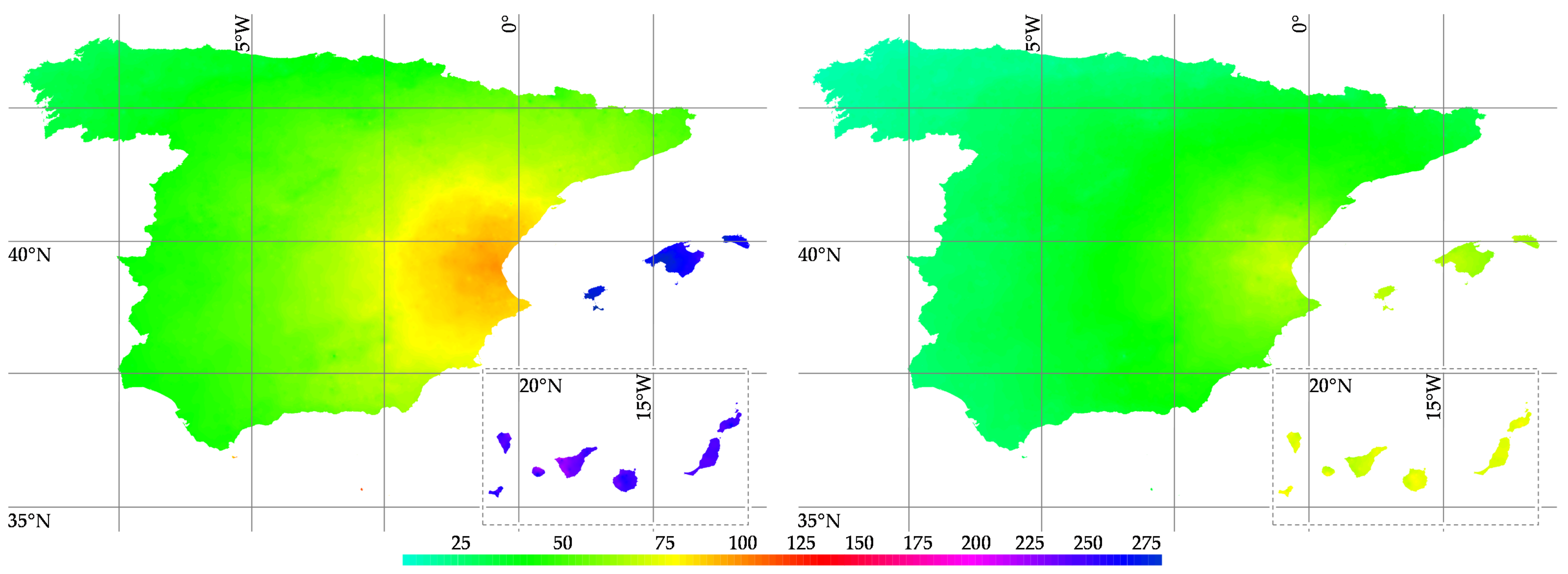
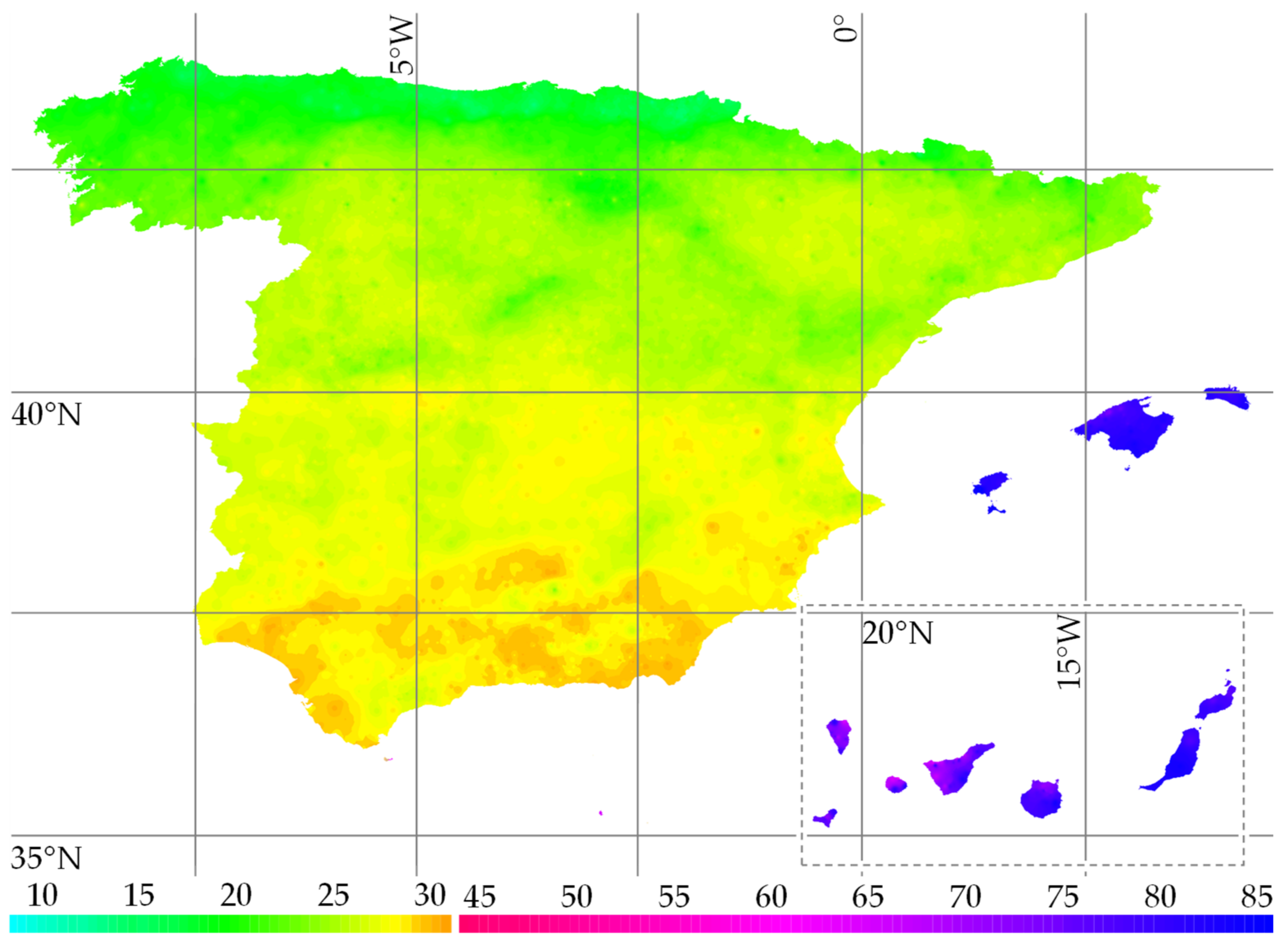
On an economic level, not all cases recover the investment in less than 30 years of lifespan, if an opportunity cost of 1% is considered. For the PV application, two extreme scenarios have been studied regarding the PV production: 100% for savings, 100% for sale. Savings range from 6.5–15.5 k €, with an average of 11 k €. However, if all the production is a surplus, the results range 0 and 3 k €, with an average of 2 k €, without no municipality with a negative balance. For the ST application, savings depend on the auxliary supply energy. If an electric boiler is the initial supplier for DHW, energy bills are reduced by 4-8 k €, with an average of 6 k €. On the contrary, if a natural gas boiler is the initial supplier, costs saved range 0–1.5 k €, with an average of 0.5 k €. In this case, the investment is not recovered in 169 municipalities (2% of the total number).

If the investment is divided by the annual energy production, an economic ratio can be obtained, as shown in

Table 20. Ratio effort in cost-energy -production for PV (left) and ST (right) installations in € cents/kWh.

Statistical Summary								Statistical Summary
Minimum	3	Average (µ)	4	Weighted µ	4	Maximum	6	Minimum	5	Average (µ)	6	Weighted µ	6	Maximum	7
Cities > 250 k Inhabitants								Cities > 250 k Inhabitants
Madrid	4	Zaragoza	4	Las Palmas	3	Cordoba	3	Madrid	6	Zaragoza	5	Las Palmas	5	Cordoba	5
Barcelona	4	Malaga	3	Bilbao	5	Valladolid	4	Barcelona	6	Malaga	5	Bilbao	7	Valladolid	5
Valencia	3	Murcia	3	Alicante	3	Vigo	4	Valencia	5	Murcia	5	Alicante	5	Vigo	6
Seville	3	Palma	4	Gijon	5	Vitoria	4	Seville	5	Palma	5	Gijon	7	Vitoria	6

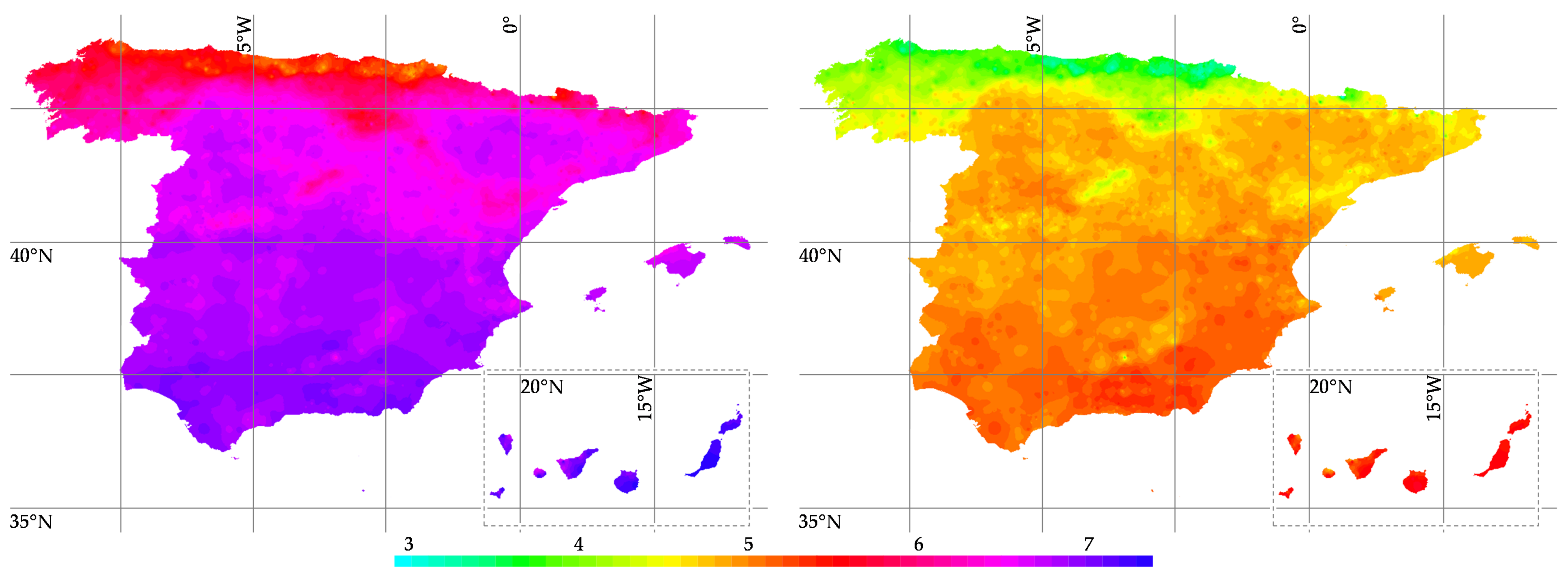
and Figure 10. These check if the cost by production (in € cents/kWh) is higher or lower than the energy (electricity or natural gas) price to be considered. For the PV saving scenario and the ST electricity one, 18.78 € cents/kWh is used for the calculations. These prices are higher than the trend indicated by Eureletric (about 19–21 € cents/kWh). For the PV surplus scenario, 6.42 € cents/kWh is used for the calculations. For the ST natural gas scenario, 7.20 € cents/kWh is used. These are lower than the trend indicated by Eureletric (about 8–9 € cents/kWh). If the ratio effort is lower than the prices considered, the initiative will be economically profitable.

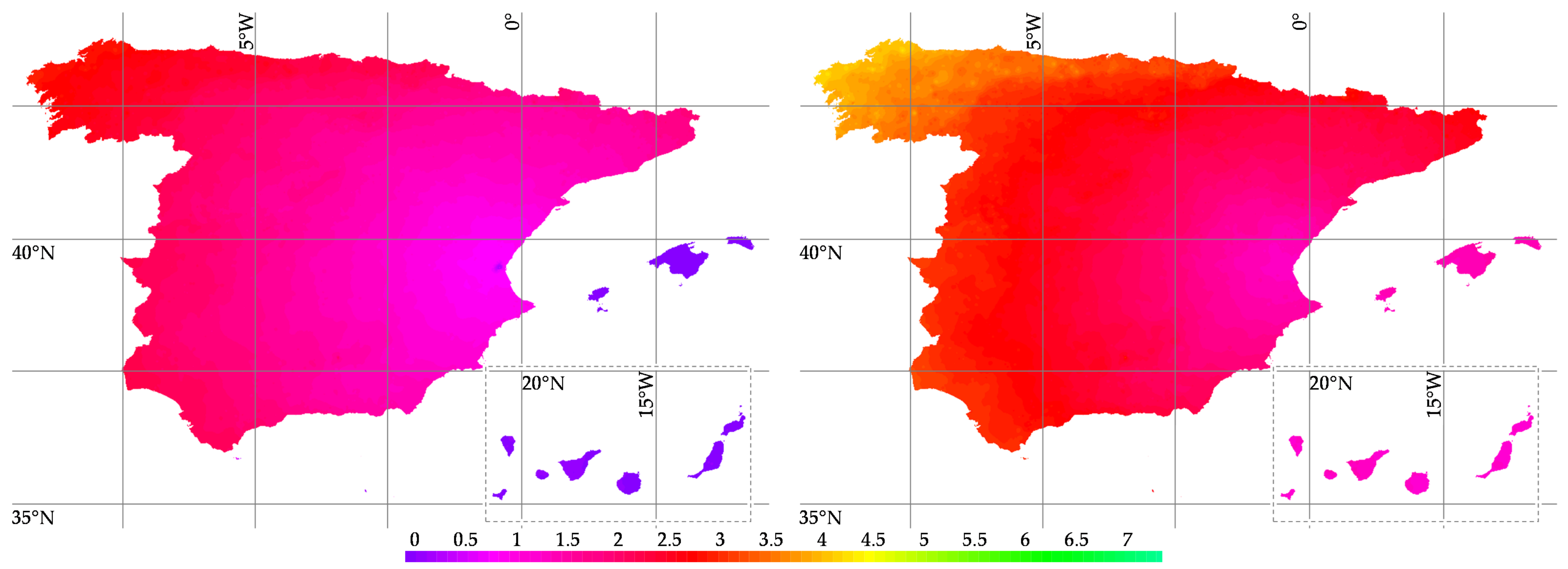
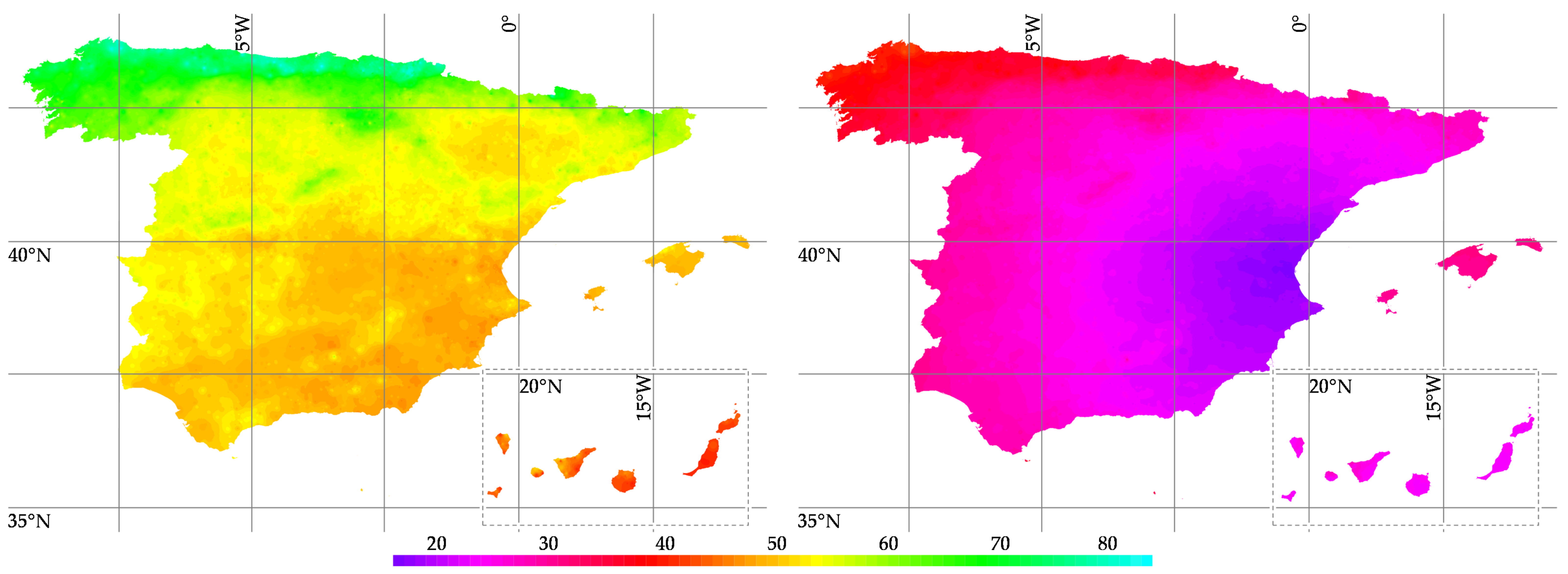
Regarding emissions, the CO₂eq emission transfer factors approved by the Permanent Commission for Energy Certification (EPC Advisory Committee) have been considered, both for electricity and natural gas, as shown in Table 11. In addition, initial, operational and maintenance emissions as a result of including a PV system and/or a ST one have also been tested. For the PV application, emmisions saved range between 15–87 tons of CO₂eq with an average of 26 tons (24 in Mainland and 78 in the islands and autonomous cities). For the ST application results depend on the auxliary supply energy. If an electric boiler is the initial supplier, the emissions saved range between 14–56 tons of CO₂eq with an average of 19 tons (18 in Mainland and 52 in the islands and autonomous cities). On the contrary, if a natural gas boiler is the initial supplier, the emissions saved range between 9–16 tons of CO₂eq (without significant differences between the Mainland and the rest of the country). Analysing the annual emissions balance, the guidelines laid out in directives EPBD-2002/91/CE (20% by 2020) and EPBD-2010/31/UE (40% by 2030) are far exceeded once more.

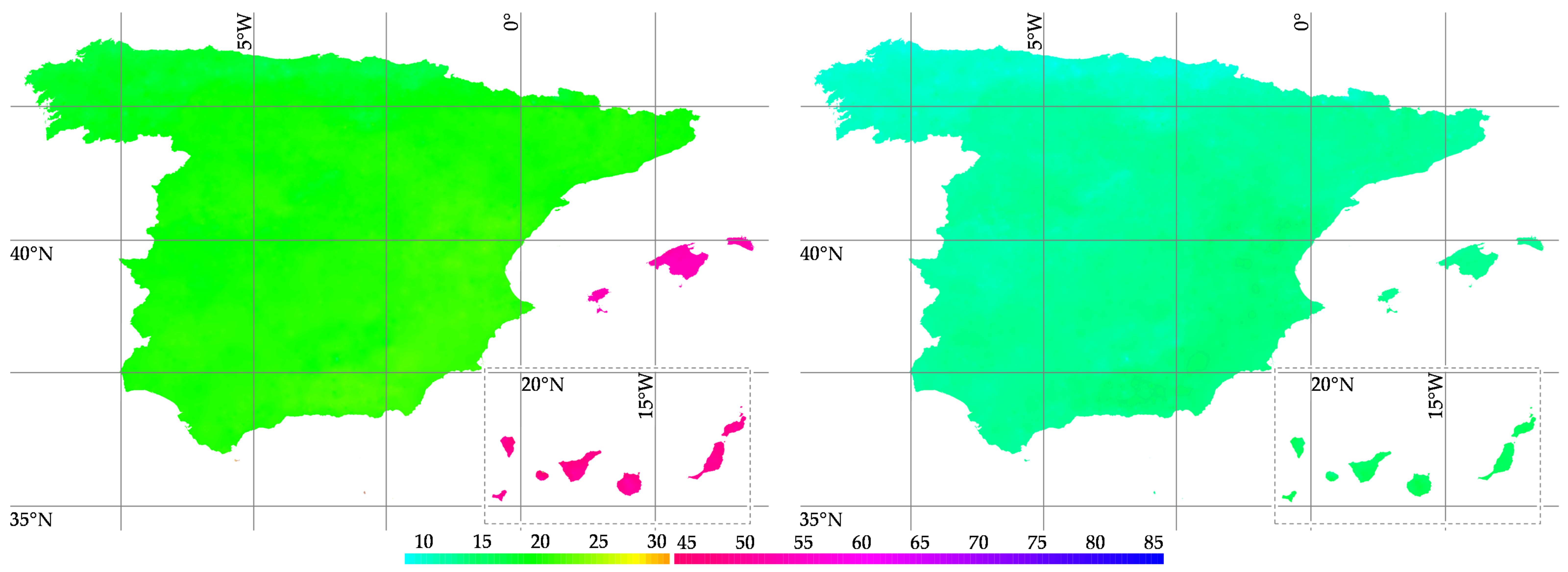
If PV and ST emissions are divided by the annual energy production, an environmental ratio is obtained, as shown in

Table 21. Ratio effort in emissions-energy production for PV (left) and ST (right) installations (in g CO₂eq/kWh).

Statistical Summary								Statistical Summary
Minimum	41.71	Average (µ)	57.29	Weighted µ	55.80	Maximum	85.56	Minimum	17.41	Average (µ)	26.98	Weighted µ	26.87	Maximum	44.62
Cities > 250 k Inhabitants								Cities > 250 k Inhabitants
Madrid	54.47	Zaragoza	52.63	Las Palmas	46.14	Cordoba	50.12	Madrid	25.26	Zaragoza	23.52	Las Palmas	25.62	Cordoba	25.81
Barcelona	56.66	Malaga	51.84	Bilbao	75.86	Valladolid	56.67	Barcelona	25.76	Malaga	27.38	Bilbao	35.09	Valladolid	28.12
Valencia	49.62	Murcia	50.20	Alicante	50.33	Vigo	66.70	Valencia	17.70	Murcia	21.10	Alicante	20.43	Vigo	37.92
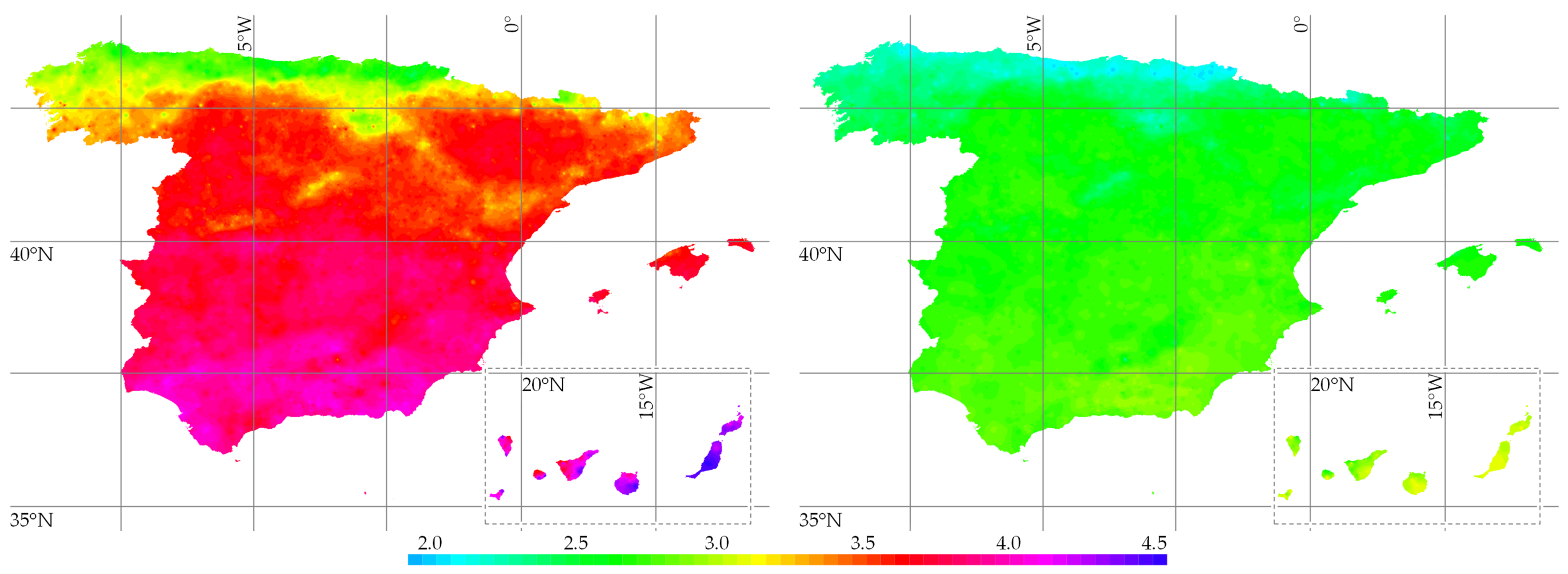
Seville	52.01	Palma	50.24	Gijon	76.87	Vitoria	66.73	Seville	28.87	Palma	30.73	Gijon	38.68	Vitoria	30.36

and Figure 11. These check if the emissions by production (in g CO₂eq/kWh) are higher or lower than the energy emissions to be considered. For S1, S2 and S3, 331 g CO₂eq/kWh in the mainland, 721 in the Autonomous Cities of Ceuta and Melilla, 932 in Balearic Island or 776 in the Canary Islands are used for the calculations. For S4, 252 g CO₂eq/kWh is used in the entire country. If the ratio effort is lower than the emissions considered, the initiative will be environmentally profitable. It can be noted that all the scenarios studied are, from this point of view, extremely promising.

If the PV and ST emissions are studied according to the lifecycle phase, weighting strongly varies from one system to another. For the PV application, the manufacturing phase ranges 78–89% of the total emissions, logistics ranges 0–12% and maintenance ranges 10–11%. On the contrary, for the ST application, the manufacturing phase ranges 27–52% of the total, logistics ranges 0–48%, operation ranges 19–64% and maintenance ranges 1–3%.

The energy efficiency of buildings has been analyzed in most Southern European countries, such as Greece [67], Italy [68], Portugal [69] and Turkey [70], as well as Spain [32,71,72]. However, these studies use cases of multifamily buildings by climatic zones or located in a specific geographic area. They are focused on comparing the primary energy consumption before and after transposition of the EPBDs, for which they usually define the envelope and calculate the heating, cooling and DHW demands. However, they usually avoid including economic or environmental issues, as well as the use of renewable energies as alternative methods of generation. In addition, most studies related to improve the energy efficiency and thus the environmental performance are focused on new buildings instead of renovation of existing ones. However, there are additional measures that can lead to further energy efficiency improvements. In this context, the inclusion of renewable energy sources arises for reducing the energy consumption, GHG emissions and energy bills. It can be noted that, although the selection of renewable sources depends largely on climate, the countries with the lowest solar potential (Northern and Central European countries) have the highest electricity and natural gas prices [73] and even some of them a higher emissions factor due to the use of carbon-based sources (for example, Germany is currently at 411 g CO₂eq/kWh according to Eurostat, about 25% higher than Spain).

Regarding the solar systems included in this research, Ref. [74] studied a domestic PV system in one municipality of France (Marseille) and two municipalities of Spain (Madrid and Seville). Their objective was to optimize the PV system by location, based on two assumptions: not returning surplus to the grid and not storing surplus energy. Despite its higher potential, the Spanish ones were dimensioned at 1.5 kWp and the French one at 2.5 kWp. This was due to four reasons: different cost of photovoltaic facilities, variable electricity prices, Spanish tax to be paid (before the entry into force of RD 244/2019) and France’s higher energy needs. In the case of Spain, the consumption was taken from the standard Spanish hourly profile provided by the Ministry of Industry. For the sake of simplicity, the PV production was obtained thanks to an online tool based on the local irradiance for each month and geographic position. Other variables influencing the PV production were also avoided.

Ref. [75] analyzed the economic and environmental impacts of substituting coal-fired electricity with PV power. The economic assessment was done through an input-output analysis, including considerations about employment, household incomes, net government tax revenue and gross domestic product that results from power generation. On the other side, the environmental analysis was based on a life cycle approach, and not only considered GHG emissions, but also SO₂, NOx and TSP emissions, and even water consumption. Geographical nuances were also excluded.

Ref. [76] reviewed 153 lifecycle studies covering a broad range of wind and solar PV electricity generation technologies to finally identify 41 of the most relevant, recent, rigorous, and original ones. Their results showed that PV energy generated a range of GHG emissions of 1 g CO₂eq/kWh to 218 g CO₂eq/kWh, where the mean value was 49.91 g CO₂eq/kWh, which are compatible with the results achieved in this research. Accordingly, although solar technologies are not “carbon-free”, they can be considered as “low-carbon”. Finally, Ref. [24] assessed a domestic ST system in the United Kingdom (UK) to measure its sustainability for partially attending the DHW demand. For the sake of simplicity, the ST production was obtained considering a national average solar irradiation and a constant efficiency was assumed.

Regarding the literature discussed, the energy simulation allows us to determine with higher precision and reliability the economic and environmental results, which is important in those locations in which results are not extremely clear and the decision must be made with more and better information. In addition, the use of a GIS technology allows a GIS-based approach to energy performance assessments of buildings at urban level. The findings of this work can be used by policymakers as guidelines for the development of national strategic plans and financial incentives for the promotion of small-scale residential solar thermal and photovoltaic applications, as well as by designers, supervisors, managers, and developers to include them in their new construction or renovation projects.

5. Conclusions

An energetic, economic and environmental life cycle assessment of two types of solar renewable energy applications (solar thermal and photovoltaic sources) has been done. The results have been estimated and compared with conventional supply systems (electricity and natural gas). The energy behavior in the initial configuration (supplied by conventional systems) is compared with that obtained after it is updated with these new facilities. This paper shows the main energy, economic and environmental indicators throughout the whole territory of Spain, considering the singularities of each location (local climatology, transportation, etc.). This GIS-based approach allows to contrast strengths and weaknesses of the systems studied from different points of view, facilitating decision making in a more holistic manner.

The results show that the European objectives are far exceeded. The energy savings achieved range from 67% to 126%, carbon dioxide emissions decrease by 42% to 100% and energy bills are reduced in cost by 32% to 81%. Therefore, solar renewable energy systems to be installed in existing or new residential buildings are essential elements to fulfill with the objective of reach nearly zero energy solutions.

This study is limited by the study of PV and ST systems manufactured in Spain (specifically in the city of Valencia), so it would be (both economically and environmentally) interesting to study the case that these are imported, for example from China. As future lines of research, the inclusion of other renewable energies, such as biomass, wind and hydrogen in the domestic environment stands out. The inclusion of end-of-life management of the systems studied, which can have an impact on categories other than climate change, is also noteworthy. Finally, to facilitate the replicability and comparison, the majority of the data analysis and spreadsheets have all been included as Supplementary Materials.

References

1. European Commission Energy Performance of Buildings Directive. Available online: https://ec.europa.eu/energy/topics/energy-efficiency/energy-efficient-buildings/energy-performance-buildings-directive_en (accessed on 20 May 2021).
2. Duarte, R.; Sánchez-Chóliz, J.; Sarasa, C. Consumer-side actions in a low-carbon economy: A dynamic CGE analysis for Spain. Energy Policy 2018, 118, 199–210. [Google Scholar] [CrossRef]
3. Merini, I.; Molina-García, A.; García-Cascales, M.S.; Ahachad, M. Energy Efficiency Regulation and Requirements: Comparison between Morocco and Spain; Springer: Cham, Switzerland, 2019; Volume 914, pp. 197–209. ISBN 978-3-030-11883-9. [Google Scholar]
4. Uihlein, A.; Eder, P. Policy options towards an energy efficient residential building stock in the EU-27. Energy Build. 2010, 42, 791–798. [Google Scholar] [CrossRef]
5. Anser, M.K.; Apergis, N.; Syed, Q.R. Impact of economic policy uncertainty on CO2 emissions: Evidence from top ten carbon emitter countries. Environ. Sci. Pollut. Res. 2021, 28, 29369–29378. [Google Scholar] [CrossRef]
6. Barthelmes, V.M.; Becchio, C.; Corgnati, S.P. Occupant behavior lifestyles in a residential nearly zero energy building: Effect on energy use and thermal comfort. Sci. Technol. Built Environ. 2016, 22, 960–975. [Google Scholar] [CrossRef]
7. European Community Directive 2002/91/EC on the energy performance of buildings. Off. J. Eur. Communities 2003, 1, 65–71.
8. European Union Directive 2010/31/EU on the energy performance of buildings. Off. J. Eur. Union 2010, 153, 13–35.
9. European Union Directive 2012/27/EU on energy efficiency. Off. J. Eur. Union 2012, 31, 1–56.
10. European Union Directive 2018/844/EU amending Directive 2010/31/EU on the energy performance of buildings and Directive 2012/27/EU on energy efficiency. Off. J. Eur. Union 2018, 156, 75–91.
11. Government of Spain Law 38/99 on Building Management. Spanish Off. Gaz. 1999, 266, 38925–38934.
12. Government of Spain Royal Decree 314/2006 on the Technical Building Code. Off. State Gaz. 2006, 74, 11816–11831.
13. Government of Spain Basic Building Standard CT-79 on thermal conditions in buildings. Off. State Gaz. 1979, 253, 24524–24550.
14. Government of Spain Royal Decree 732/2019 modifying the Technical Building Code. Off. State Gaz. 2019, 311, 140488–140674.
15. Government of Spain Royal Decree 244/2019 regulating the administrative, technical and economic conditions of electricity self-consumption. Off. State Gaz. 2019, 83, 35674–35719.
16. Muteri, V.; Cellura, M.; Curto, D.; Franzitta, V.; Longo, S.; Mistretta, M.; Parisi, M.L. Review on Life Cycle Assessment of Solar Photovoltaic Panels. Energies 2020, 13, 252. [Google Scholar] [CrossRef] [Green Version]
17. De Luca, G.; Ballarini, I.; Lorenzati, A.; Corrado, V. Renovation of a social house into a NZEB: Use of renewable energy sources and economic implications. Renew. Energy 2020, 159, 356–370. [Google Scholar] [CrossRef]
18. Ritchie, H.; Roser, M. Renewable Energy. Our World in Data. 2020. Available online: https://ourworldindata.org/renewable-energy (accessed on 15 December 2020).
19. Fortune Business Insights. Solar Thermal. Global Market Analysis, Insights and Forecast, 2015–2026; Fortune Business Insights: Pune, India, 2018. [Google Scholar]
20. García-Sanz-Calcedo, J.; López-Rodríguez, F. Analysis on the performance of a high efficiency administrative building in Spain. Int. J. Green Energy 2017, 14, 55–62. [Google Scholar] [CrossRef]
21. Heinbach, K.; Hirschl, B.; Salecki, S. Value-Added and Employment Effects of Renewable Energies and the Energy-Efficiency Refurbishment of Existing Housing—Case Study: Berlin, Germany. In Urban Energy Transition. Renewable Strategies for Cities and Regions; Droege, P., Ed.; Elsevier: Amsterdam, The Netherlands, 2018; pp. 457–466. ISBN 978-0081020746. [Google Scholar]
22. Bernath, C.; Deac, G.; Sensfuß, F. Impact of sector coupling on the market value of renewable energies—A model-based scenario analysis. Appl. Energy 2021, 281, 115985. [Google Scholar] [CrossRef]
23. De la Cruz-Lovera, C.; Perea-Moreno, A.-J.; de la Cruz-Fernández, J.-L.; Alvarez-Bermejo, J.; Manzano-Agugliaro, F. Worldwide Research on Energy Efficiency and Sustainability in Public Buildings. Sustainability 2017, 9, 1294. [Google Scholar] [CrossRef] [Green Version]
24. Greening, B.; Azapagic, A. Domestic solar thermal water heating: A sustainable option for the UK? Renew. Energy 2014, 63, 23–36. [Google Scholar] [CrossRef]
25. Mahmud, M.; Huda, N.; Farjana, S.; Lang, C. Environmental Impacts of Solar-Photovoltaic and Solar-Thermal Systems with Life-Cycle Assessment. Energies 2018, 11, 2346. [Google Scholar] [CrossRef] [Green Version]
26. Lamnatou, C.; Motte, F.; Notton, G.; Chemisana, D.; Cristofari, C. Building-integrated solar thermal system with/without phase change material: Life cycle assessment based on ReCiPe, USEtox and Ecological footprint. J. Clean. Prod. 2018, 193, 672–683. [Google Scholar] [CrossRef]
27. Horan, P.; Luther, M.B.; Li, H.X. Guidance on Implementing Renewable Energy Systems in Australian Homes. Energies 2021, 14, 2666. [Google Scholar] [CrossRef]
28. Mehrjerdi, H.; Iqbal, A.; Rakhshani, E.; Torres, J.R. Daily-seasonal operation in net-zero energy building powered by hybrid renewable energies and hydrogen storage systems. Energy Convers. Manag. 2019, 201, 112156. [Google Scholar] [CrossRef]
29. García-Sanz-Calcedo, J.; Al-Kassir, A.; Yusaf, T. Economic and Environmental Impact of Energy Saving in Healthcare Buildings. Appl. Sci. 2018, 8, 440. [Google Scholar] [CrossRef] [Green Version]
30. Chastas, P.; Theodosiou, T.; Bikas, D.; Tsikaloudaki, K. Integrating embodied impact into the context of EPBD recast: An assessment on the cost-optimal levels of nZEBs. Energy Build. 2020, 215, 109863. [Google Scholar] [CrossRef]
31. Milousi, M.; Souliotis, M.; Arampatzis, G.; Papaefthimiou, S. Evaluating the Environmental Performance of Solar Energy Systems Through a Combined Life Cycle Assessment and Cost Analysis. Sustainability 2019, 11, 2539. [Google Scholar] [CrossRef] [Green Version]
32. López-Ochoa, L.M.; Las-Heras-Casas, J.; López-González, L.M.; Olasolo-Alonso, P. Environmental and energy impact of the EPBD in residential buildings in hot and temperate Mediterranean zones: The case of Spain. Energy 2018, 161, 618–634. [Google Scholar] [CrossRef]
33. Nejat, P.; Jomehzadeh, F.; Taheri, M.M.; Gohari, M.; Majid, M.Z.A. A global review of energy consumption, CO2 emissions and policy in the residential sector (with an overview of the top ten CO2 emitting countries). Renew. Sustain. Energy Rev. 2015, 43, 843–862. [Google Scholar] [CrossRef]
34. Cerezo-Narváez, A.; Piñero-Vilela, J.M.; Rodríguez-Jara, E.Á.; Otero-Mateo, M.; Pastor-Fernández, A.; Ballesteros-Pérez, P. Transformation of residential housings from the real estate bubble into nearly zero-energy buildings: Case studies. DYNA 2020, 95, 674–680. [Google Scholar] [CrossRef]
35. Pombo, O.; Allacker, K.; Rivela, B.; Neila, J. Sustainability assessment of energy saving measures: A multi-criteria approach for residential buildings retrofitting—A case study of the Spanish housing stock. Energy Build. 2016, 116, 384–394. [Google Scholar] [CrossRef] [Green Version]
36. Soto, T.; Escrig, T.; Serrano-Lanzarote, B.; Matarredona Desantes, N. An Approach to Environmental Criteria in Public Procurement for the Renovation of Buildings in Spain. Sustainability 2020, 12, 7590. [Google Scholar] [CrossRef]
37. Monzón-Chavarrías, M.; López-Mesa, B.; Resende, J.; Corvacho, H. The nZEB concept and its requirements for residential buildings renovation in Southern Europe: The case of multi-family buildings from 1961 to 1980 in Portugal and Spain. J. Build. Eng. 2021, 34, 101918. [Google Scholar] [CrossRef]
38. Zhang, C.; Hu, M.; Laclau, B.; Garnesson, T.; Yang, X.; Li, C.; Tukker, A. Environmental life cycle costing at the early stage for supporting cost optimization of precast concrete panel for energy renovation of existing buildings. J. Build. Eng. 2021, 35, 102002. [Google Scholar] [CrossRef]
39. Vourdoubas, J. Creation of Zero CO2 Emissions Residential Buildings due to Operating and Embodied Energy Use on the Island of Crete, Greece. Open J. Energy Effic. 2017, 6, 141–154. [Google Scholar] [CrossRef] [Green Version]
40. Rey-Hernández, J.M.; Velasco-Gómez, E.; San José-Alonso, J.F.; Tejero-González, A.; Rey-Martínez, F.J. Energy Analysis at a Near Zero Energy Building. A Case-Study in Spain. Energies 2018, 11, 857. [Google Scholar] [CrossRef] [Green Version]
41. Cunha, F.O.; Oliveira, A.C. Benchmarking for realistic nZEB hotel buildings. J. Build. Eng. 2020, 30, 101298. [Google Scholar] [CrossRef]
42. Palomba, V.; Borri, E.; Charalampidis, A.; Frazzica, A.; Karellas, S.; Cabeza, L.F. An Innovative Solar-Biomass Energy System to Increase the Share of Renewables in Office Buildings. Energies 2021, 14, 914. [Google Scholar] [CrossRef]
43. Garcia Latorre, F.J.; Quintana, J.J.; de la Nuez, I. Technical and economic evaluation of the integration of a wind-hydro system in El Hierro island. Renew. Energy 2019, 134, 186–193. [Google Scholar] [CrossRef]
44. Ghazvini, M.; Sadeghzadeh, M.; Ahmadi, M.H.; Moosavi, S.; Pourfayaz, F. Geothermal energy use in hydrogen production: A review. Int. J. Energy Res. 2019, 43, 7823–7851. [Google Scholar] [CrossRef]
45. Ala, G.; Di Filippo, G.; Viola, F.; Giglia, G.; Imburgia, A.; Romano, P.; Castiglia, V.; Pellitteri, F.; Schettino, G.; Miceli, R. Different Scenarios of Electric Mobility: Current Situation and Possible Future Developments of Fuel Cell Vehicles in Italy. Sustainability 2020, 12, 564. [Google Scholar] [CrossRef] [Green Version]
46. Hazim, S.; Salih, A.; Taha Janan, M.; El Ouatouati, A.; Ghennioui, A. Marine current energy assessment and the hydrodynamic design of the hydrokinetic turbine for the Moroccan Mediterranean Coast. Energy Explor. Exploit. 2021, 39, 717–737. [Google Scholar] [CrossRef]
47. Huld, T.; Müller, R.; Gambardella, A. A new solar radiation database for estimating PV performance in Europe and Africa. Sol. Energy 2012, 86, 1803–1815. [Google Scholar] [CrossRef]
48. Mueller, R.; Behrendt, T.; Hammer, A.; Kemper, A. A New Algorithm for the Satellite-Based Retrieval of Solar Surface Irradiance in Spectral Bands. Remote Sens. 2012, 4, 622–647. [Google Scholar] [CrossRef] [Green Version]
49. Gracia Amillo, A.; Huld, T.; Müller, R. A New Database of Global and Direct Solar Radiation Using the Eastern Meteosat Satellite, Models and Validation. Remote Sens. 2014, 6, 8165–8189. [Google Scholar] [CrossRef] [Green Version]
50. Endesa Electricity Tariffs. Available online: https://www.endesa.com/en/catalog/light (accessed on 15 December 2020).
51. Iberdrola Electricity Plans. Available online: https://www.iberdrola.es/en/electricity (accessed on 15 December 2020).
52. Naturgy Tarifas de Gas (Gas Tariffs). Available online: https://www.naturgy.es/hogar/gas (accessed on 15 December 2020).
53. Repsol Gas & Más (Gas & More). Available online: https://www.repsolluzygas.com/gas-y-mas/ (accessed on 15 December 2020).
54. European Union Energy Prices. Available online: https://ec.europa.eu/eurostat/statistics-explained/index.php?title=Category:Energy_prices (accessed on 20 March 2021).
55. Capros, P.; De Vita, A.; Tasios, N.; Chanioti, X.; Papadopoulos, D. Power Choices Reloaded; Eurelectric: Athens, Greece, 2013. [Google Scholar]
56. CYPE Engineers. Arquimedes Software Version 2021.f; CYPE Engineers: Alacant, Spain, 2021; Available online: http://www.cype.es/ (accessed on 15 December 2020).
57. Leduc, S.; Liu, Z. The Uncertainty Channel of the Coronavirus; Federal Reserve Bank of San Francisco: San Francisco, CA, USA, 2020; Available online: https://www.frbsf.org/economic-research/publications/economic-letter/2020/march/uncertainty-channel-of-coronavirus/ (accessed on 15 December 2020).
58. EcoInvent EcoInvent 3.3. Available online: https://www.ecoinvent.org/database/older-versions/ecoinvent-33/ecoinvent-33.html (accessed on 30 April 2021).
59. Intergovernmental Panel on Climate Change. Climate Change 2013—The Physical Science Basis; Intergovernmental Panel on Climate Change, Ed.; Cambridge University Press: Cambridge, UK, 2014; ISBN 978-1107415324. [Google Scholar]
60. Government of Spain. CO2 Emission Factors and Primary Energy Conversion Coefficients of Different Final Energy Sources Consumed in the Building Sector in Spain; Ministry of Industry, Energy and Tourism and Ministry of Public Works: Madrid, Spain, 2016.
61. Solar Energy Laboratory. TRNSYS Transient System Simulation Tool version 17; University of Wisconsin-Madison: Madison, WI, USA, 2012; Available online: https://sel.me.wisc.edu/trnsys/ (accessed on 15 December 2020).
62. Beccali, M.; Cellura, M.; Fontana, M.; Longo, S.; Mistretta, M. Energy retrofit of a single-family house: Life cycle net energy saving and environmental benefits. Renew. Sustain. Energy Rev. 2013, 27, 283–293. [Google Scholar] [CrossRef]
63. Solar Energy Laboratory. Manual of TRNSYS 17 a TRaNsient System Simulation Program; University of Wisconsin-Madison: Madison, WI, USA, 2012; Volume 5. [Google Scholar]
64. ESRI. ArcGIS Desktop Version 10.6.1; ESRI: Redlands, CA, USA, 2019; Available online: https://desktop.arcgis.com/en/ (accessed on 15 December 2020).
65. The Spanish Electricity System. How Much Do My Household Appliances Consume? The Spanish Electricity System: Madrid, Spain, 2020; Available online: https://www.ree.es/sites/default/files/interactivos/como_consumimos_electricidad/cuanto-consumen-mis-electrodomesticos.html (accessed on 15 December 2020).
66. European Commission. Guide to Cost-Benefit Analysis of Investment Projects: Economic Appraisal Tool for Cohesion Policy 2014–2020; Publications Office of the European Union: Brussels, Belgium, 2014; ISBN 9789279347962. [Google Scholar] [CrossRef]
67. Gaglia, A.G.; Tsikaloudaki, A.G.; Laskos, C.M.; Dialynas, E.N.; Argiriou, A.A. The impact of the energy performance regulations’ updated on the construction technology, economics and energy aspects of new residential buildings: The case of Greece. Energy Build. 2017, 155, 225–237. [Google Scholar] [CrossRef]
68. Salvalai, G.; Masera, G.; Sesana, M.M. Italian local codes for energy efficiency of buildings: Theoretical definition and experimental application to a residential case study. Renew. Sustain. Energy Rev. 2015, 42, 1245–1259. [Google Scholar] [CrossRef]
69. Magalhães, S.M.C.; Leal, V.M.S. Characterization of thermal performance and nominal heating gap of the residential building stock using the EPBD-derived databases: The case of Portugal mainland. Energy Build. 2014, 70, 167–179. [Google Scholar] [CrossRef]
70. Kalaycıoğlu, E.; Yılmaz, A.Z. A new approach for the application of nearly zero energy concept at district level to reach EPBD recast requirements through a case study in Turkey. Energy Build. 2017, 152, 680–700. [Google Scholar] [CrossRef]
71. López-Ochoa, L.M.; Las-Heras-Casas, J.; López-González, L.M.; García-Lozano, C. Environmental and energy impact of the EPBD in residential buildings in cold Mediterranean zones: The case of Spain. Energy Build. 2017, 150, 567–582. [Google Scholar] [CrossRef]
72. Bastante-Ceca, M.J.; Cerezo-Narváez, A.; Piñero-Vilela, J.M.; Pastor-Fernández, A. Determination of the Insulation Solution that Leads to Lower CO2 Emissions during the Construction Phase of a Building. Energies 2019, 12, 2400. [Google Scholar] [CrossRef] [Green Version]
73. D’Agostino, D.; Parker, D. A framework for the cost-optimal design of nearly zero energy buildings (NZEBs) in representative climates across Europe. Energy 2018, 149, 814–829. [Google Scholar] [CrossRef]
74. Arcos-Vargas, A.; Cansino, J.M.; Román-Collado, R. Economic and environmental analysis of a residential PV system: A profitable contribution to the Paris agreement. Renew. Sustain. Energy Rev. 2018, 94, 1024–1035. [Google Scholar] [CrossRef]
75. Wang, Z.; Fan, W. Economic and environmental impacts of photovoltaic power with the declining subsidy rate in China. Environ. Impact Assess. Rev. 2021, 87, 106535. [Google Scholar] [CrossRef]
76. Nugent, D.; Sovacool, B.K. Assessing the lifecycle greenhouse gas emissions from solar PV and wind energy: A critical meta-survey. Energy Policy 2014, 65, 229–244. [Google Scholar] [CrossRef]
Figure 2. Location of 8131 municipalities of Spain (highlighting cities > 250 k inhabitants).
Energies 14 04183 g002
Figure 3. PV (up) and ST (down) production ordered by latitude (left) and solar radiation (right).
Energies 14 04183 g003
Figure 4. Contribution to electricity consumption in % excluding DHW (PV left), and contribution to DHW consumption (ST right).
Energies 14 04183 g004
Figure 5. Contribution to household consumption in % combining PV and ST.
Energies 14 04183 g005
Figure 6. PV IRR in % (S1 (consumption saving scenario) left, S2 (surplus sale scenario) right).
Energies 14 04183 g006
Figure 7. ST IRR in % (S3 (auxiliary electricity supply scenario) left, S4 (auxiliary natural gas supply scenario) right).
Energies 14 04183 g007
Figure 8. PV ERR in % (S1 (consumption saving scenario) and S2 (surplus sale scenario)).
Energies 14 04183 g008
Figure 9. ST ERR in % (S3 (auxiliary electricity supply scenario) left, and S4 (auxiliary natural gas supply scenario) right).
Energies 14 04183 g009
Figure 10. Ratio effort in cost-energy production for PV (left) and ST (right) installations in € cents/kWh.
Energies 14 04183 g010
Figure 11. Ratio effort in emissions-energy production for PV (left) and ST (right) installations (in g CO2eq/kWh).
Energies 14 04183 g011