Article

Analyzing Trade in Continuous Intra-Day Electricity Market: An Agent-Based Modeling Approach

1
Division of Electric Power and Energy Systems, KTH Royal Institute of Technology, 11428 Stockholm, Sweden
2
Department of Electrical Engineering and Computer Science, University of Liège, 4000 Liège, Belgium
*
Author to whom correspondence should be addressed.
These authors contributed equally to this work.
Energies 2021, 14(13), 3860; https://doi.org/10.3390/en14133860
Submission received: 17 April 2021 / Revised: 3 June 2021 / Accepted: 22 June 2021 / Published: 27 June 2021

Abstract

:
In recent years, the vast penetration of renewable energy sources has introduced a large degree of uncertainty into the power system, thus leading to increased trading activity in the continuous intra-day electricity market. In this paper, we propose an agent-based modeling framework to analyze the behavior and the interactions between renewable energy sources, consumers and thermal power plants in the European Continuous Intra-day (CID) market. Additionally, we propose a novel adaptive trading strategy that can be used by the agents that participate in CID market. The agents learn how to adapt their behavior according to the arrival of new information and how to react to changing market conditions by updating their willingness to trade. A comparative analysis was performed to study the behavior of agents when they adopt the proposed strategy as opposed to other benchmark strategies. The effects of unexpected outages and information asymmetry on the market evolution and the market liquidity were also investigated.

1. Introduction

In recent decades, an increase in the share of variable renewable energy sources (RES) has been observed in the energy mix. These energy sources are characterized by highly volatile generation profiles throughout the year, as highlighted by [1], and have stimulated a substantial growth in the volumes of electricity traded in the short-term electricity markets, as pointed out by [2]. Short-term markets are organized in a sequence of trading floors [3]. First, the day-ahead (DA) market takes place one day before the physical delivery, followed by the intra-day (ID) market, where electricity trading occurs until a few minutes before the actual electricity production/consumption. Once the ID market closes, the committed generation or consumption becomes financially binding for market participants. In the case of deviations (imbalances) between the actual and the committed production/consumption, financial penalties might ensue during the imbalance settlement process. In this context, the ID trading floor becomes particularly interesting because participants can exploit the enhanced accuracy of forecasts that comes with reduced lead times. Thus, market actors can reduce their imbalances by performing adjustments close to the time of delivery as discussed by [4]. Additionally, they can provide flexibility in the market, mitigating the need for expensive balancing actions, which is further discussed by [5,6]. Intra-day markets are typically organized according to two distinct mechanisms, namely continuous trade or discrete auctions. This paper focuses on the former mechanism, as it is the one expected to prevail at the European level, as pointed out by [7,8].
The increased amount of activity expected in ID markets raises the volatility and cross-border flows in the market [3]. As a result, the need for automation in the trading process is rising. Moreover, an expected upsurge in the amount of available information and IT infrastructure for traders, which is further explained by [9,10], has prompted the development of bots for automated trading as shown by [11]. For instance, according to [12], in July 2019, the intra-day volume traded on the Nord Pool trading platform by bots through the application programming interface (API) exceeded 52%. In this context, it becomes relevant to analyze the interactions of the automated players in the ID market and evaluate their impact on the market outcome.
With reference to the increased relevance of short-term markets and automatic trading, this paper tackles the issue faced by an agent trading in the European Continuous Intraday (CID) market. In particular, we propose an open source agent-based modeling (ABM) framework for the CID market where agents can interact and exchange energy through a centralized limit order book. These agents exchange electricity according to some trading strategy. In this paper, we propose a trading strategy based on adaptive learning—such a strategy allows the agents to build price–volume curves, which are then used to post orders in the CID market. To benchmark the proposed adaptive learning trading strategy, we introduce a second one following a “naive” approach. We leverage these two strategies to assess the impact of different trading strategies on the prices of the CID market and revenues of the agents.
The presented modeling framework enables the analysis of a number of additional events and their impact on the CID markets. In this regard, we analyze the combined impact of (i) generation/consumption capacity outages and (ii) the different strategies adopted by each agent, on the price volatility in the CID market. Additionally, we investigate how some agents can influence the transaction prices in the CID market if better estimates of the imbalance prices are available those agents. Indeed, when the transmission system operator mobilizes resources to provide additional reserves in the balancing market, only some of the market players are activated. Such agents, therefore, receive information concerning reserve activation prices which is not universally available. This creates information asymmetry concerning imbalance prices across the market players.
The rest of the paper is organized as follows. Section 2 discusses the related work in the literature. Section 3 gives the overview of how the continuous ID electricity market works. The details of the proposed model are covered in the sections ranging from Section 4 to Section 7. The continuous market clearing performed by the MO is described in Section 4. The detailed modeling of different agents is explained in Section 5. Section 6 describes the pricing and volume strategies for the agents. The imbalance settlement mechanism adopted in the simulator is highlighted in Section 7. Discussions regarding the performed case studies and obtained results are given in Section 8. Section 9 concludes the paper and discusses future work avenues.

2. Related Works

The prevailing literature on energy exchange optimization has mainly focused on the DA market. As for ID and CID, limited research work can be found to date, in particular, related to the mathematical modeling of the CID electricity market. The research gap and the need to develop more detailed simulation models for the CID market is highlighted by [13]. The participation of a wind power producer (WPP) in the CID market and the benefits obtained through the reduction in the imbalance costs are presented by [14]. However, this work does not explicitly model the trading process in the ID market, and only considers a limited order book (a compilation of available bids and asks for trading). More thorough modeling of the CID market is provided by [15], where a deep reinforcement learning framework for the participation of energy storage in the CID market is proposed. In the latter, historical limit order book data were used to train the trading agent. However, the use of historical data does not allow the study of the market impact of each player. The need to model the interactions of the different market agents in the ID market has been emphasized by [16]. Similarly, Ref. [17] organized the CID electricity market as a continuous double auction (CDA) (according to [18], CDA is a fixed-duration auction mechanism where more than one buyer and seller can compete with each other to buy and sell goods, respectively, and transactions can take place at any time whenever an offer to buy and an offer to sell match) with the aim of understanding the impact of RES agents’ forecast errors on the CID market. However, their work assumes that a single entity aggregates the entire wind and solar power generation and trades the overall forecast error in the ID market as a single entity. This entity is not allowed to submit orders, but it has to accept the best price available when it enters the market.
Agent-based modeling provides a framework for simulating the operation of electricity markets, with the purpose of investigating the behavior of different market participants and to study their interactions. Some of the agent-based models (ABMs) that have been developed in the past include EMCAS (electricity market complex adaptive systems) by [19,20], NEMSIM (national electricity market simulation system) by [21], STEMS-RT (short-term electricity market simulator–real time) by [22], SEPIA (simulator for electric power industry agents) by [23], AMES (agent-based modeling of electricity system) by [24], and MASCEM (multi-agent system that simulates competitive electricity markets) by [25]. A detailed literature review of these models has been performed by [26]. Some recent research work on agent-based modeling includes [27,28,29,30,31]. A literature review of contemporary ABMs in different electricity markets can be found in [32]. However, none of the aforementioned ABMs is well suited for modeling the European CID market since the trading mechanism (limit order book) and the rules are not explicitly considered.
In this work, we present a novel ABM framework for the CID market, where all the agents can interact and exchange energy via submitting orders in a centralized limit order book. However, we adopt a different approach with respect to [33,34], where the authors proposed a model to optimize the participation of a portfolio of assets in the energy markets, aiming to maximize returns and the minimization of the implied risk. In this paper, we consider each agent to control only one type of asset. Two different pricing strategies are considered according to which the agents are posting orders in the market. The first one is a simple strategy that randomly assigns a price to the volume that each agent needs to trade at each step. The second pricing strategy adopted in this paper is a slightly modified version of the trader AA (adaptive aggressiveness) strategy presented by [35] that is used in financial markets. The main feature of this strategy is the notion of aggressiveness, which is a variable that determines the behavior of the trader in the market, e.g., passive, active, aggressive. More specifically, an aggressive trader tends to submit better offers than its estimate of the competitive equilibrium price with the intention of improving its chance of transacting. This variable is progressively learned in response to the market events. According to [36], the trader AA strategy has been shown to dominate not only all other algorithmic strategies but also human traders. However, the quoted volume is not considered as a strategic variable in this strategy. In this paper, we propose an adjusted version of the trader AA strategy that we call the modified trader AA (MTAA) strategy. The proposed strategy also uses the aggressiveness variable for the construction of price–volume curves.
In light of the above, the contributions of this paper are four-fold. First, we propose a novel ABM framework to investigate the interactions between different agents in the context of a CID market. Second, we employ an MTAA pricing strategy that learns from past events in the CID market and benchmark it against a naive strategy that randomly chooses prices from a range of prices based on the best buying and selling prices in the CID market. Third, we study the response of different agents interacting in the CID market to capacity outages under different pricing strategies. Lastly, we investigate the impact of information asymmetry of the imbalance prices on the CID market prices.

3. Principles of Continuous Intra-Day Markets
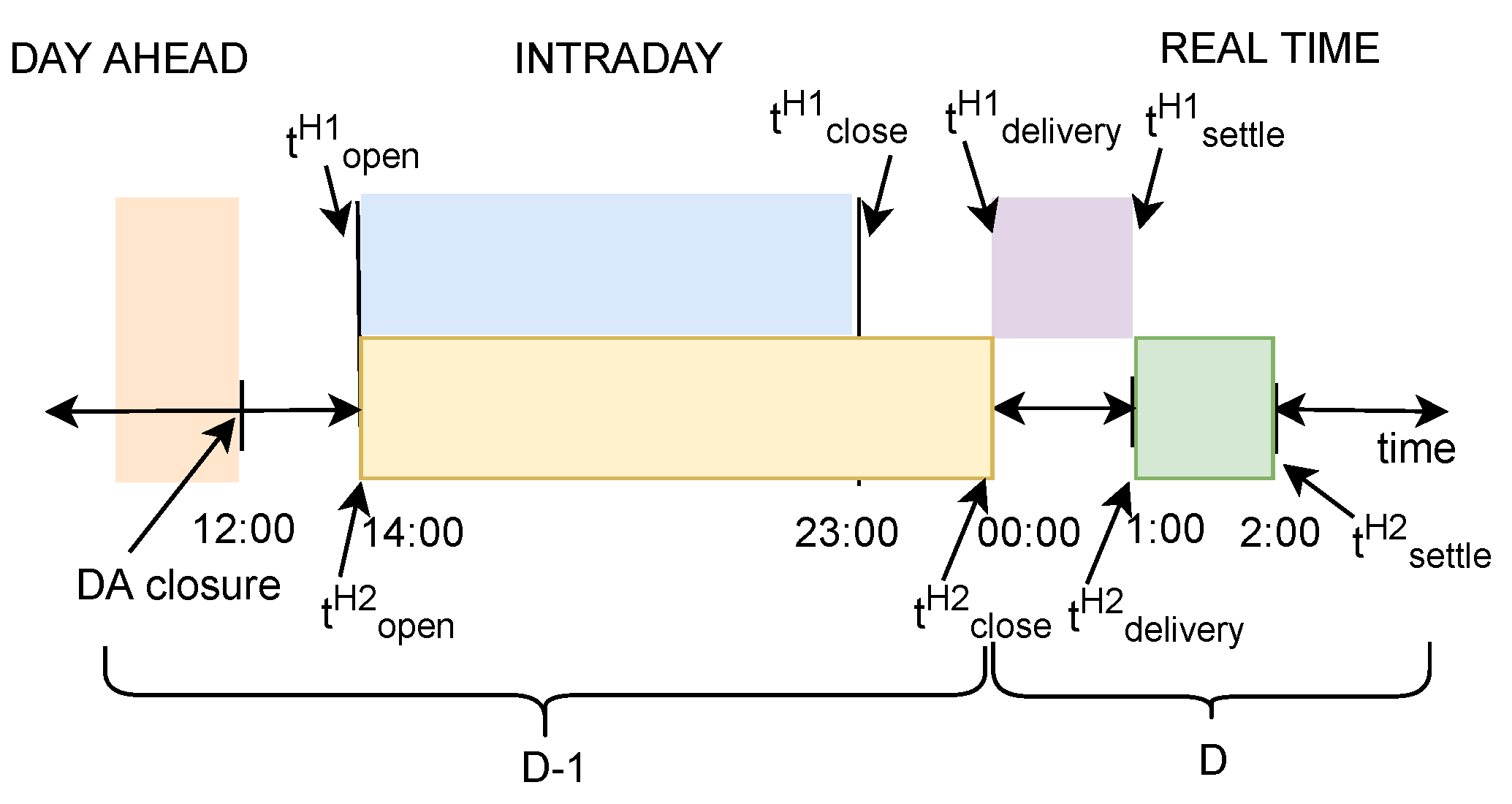
This section describes the organization and the main principles that define the exchanges in the proposed CID market mechanisms. These principles are inspired by the work of Boukas et al.; for more details, we refer the reader to [15].

3.1. Market Set-Up

In the CID market, the actual delivery of energy in a predefined time slot is known as a market product. A wide range of products is offered by the market operators in Europe based on the associated duration of physical delivery. For instance, Nord Pool offers quarterly (15 min-long), half-hourly (30 min-long), hourly, and block products. The latter are products inter-linked in time and comprise several consecutive hourly products (up to 24) as described by [37]. Although the increasing number and range of available products aim to facilitate trading activities, these also complicate the decision process.
Assumption 1.
Throughout this paper, it is considered that trading takes place solely for one product. This assumption seeks to simplify notation and to reduce the complexity arising from (i) the time coupling of the products in the delivery timeline, as well as (ii) the dependency between trading and delivery timelines.
In this regard, the market product starting at the first hour of the day can be encoded as H 1 , as shown in Figure 1. In this figure, the physical delivery of product H 1 starts at t d e l i v e r y H 1 and ends at t s e t t l e H 1 . The trading activity for this product starts the day before at t o p e n H 1 and terminates shortly before the actual delivery at t c l o s e H 1 . In the following, we will consider the trading timeline defined as the time interval T ˜ = t o p e n H 1 , t c l o s e H 1 . Furthermore, we consider a discretization of the continuous time interval T ˜ , with the discretization step Δ t . The discrete time horizon is defined as T = { t o p e n H 1 , t o p e n H 1 + Δ t , . . . , t c l o s e H 1 } .

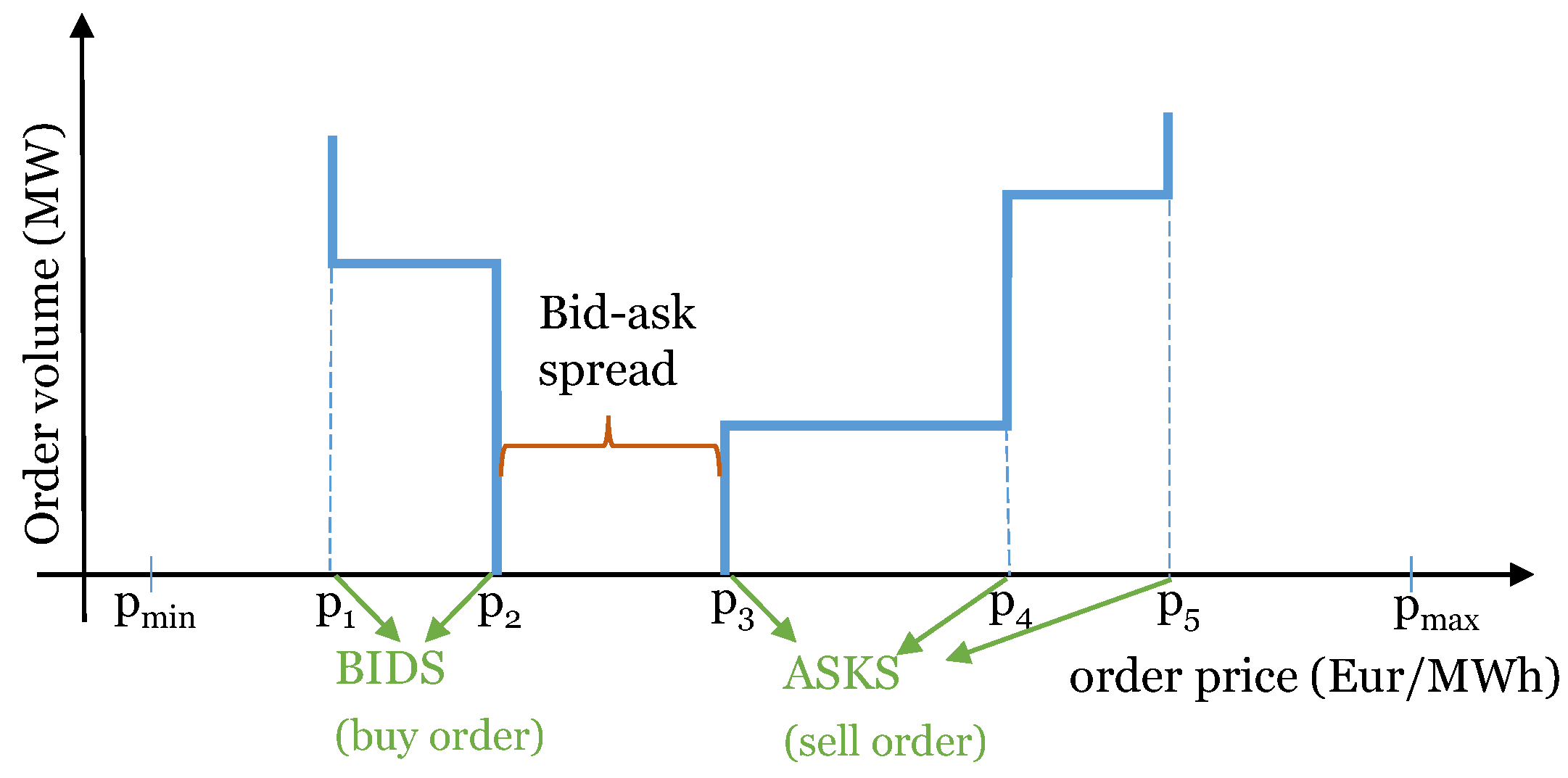
3.2. Market Mechanism

At each time-step in the trading timeline, a market participant can express their willingness to buy or sell a product (consume or produce energy during a predefined time-slot) by posting orders in the CID market. There are four main types of orders: (i) the market order, where no price limit is specified and the order is matched at the best price; (ii) the limit order, which contains a price limit and can only be matched at the specified price or better; (iii) the market sweep order, which is immediately executed (fully or partially) or canceled; and (iv) block orders, consisting of one or several (up to 24) consecutive hourly products. Each one of these types of order can receive additional execution specifications related to the time or the volume of the order execution.
Assumption 2.
In this paper, it is assumed that the agents can only place simple limit orders. Placing a new limit order for a product in the CID market involves specifying its side, i.e., whether it is a buy or a sell order y { S e l l , B u y } , its volume v R + , and the price π [ π m i n , π m a x ] for producing or consuming one unit of energy.
Every incoming order is treated according to the first-come–first-serve (FCFS) rule as explained by [38]. If the price of a new Buy (Sell) order is equal or higher (lower) than the price of an existing Sell (Buy) order, it will automatically be realized. Each transaction is settled following the pay-as-bid principle, according to which the transaction price is set by the oldest order of the two. Unmatched orders are stored in the limit order book (LOB), a ledger that centralizes all outstanding bids and asks—i.e., the pending orders that have not yet been canceled by the agents that originated them—and which is accessible to all market participants. The LOB typically has two sides, namely the bid and the ask sides. The former contains the prices and quantities of outstanding bid orders sorted in descending order, while the latter stores the prices of outstanding asks and the associated quantities sorted in ascending order. A visualization of outstanding bids and asks for product H 1 , as found in a typical LOB is presented in Figure 2. The current work follows the LOB implementation described by [39].

4. Continuous Market Clearing

This section describes the functionality of the market operator (MO) agent. The MO is responsible for organizing and facilitating the interactions between trading agents in the CID market. As previously described, the exchanges take place through a centralized order book. The MO is responsible for receiving the incoming orders from the agents, processing them, and record the financial transactions. This agent is also responsible for updating the order book and communicating it to the market participants. An overview of the CID market simulator is shown in Figure 3.

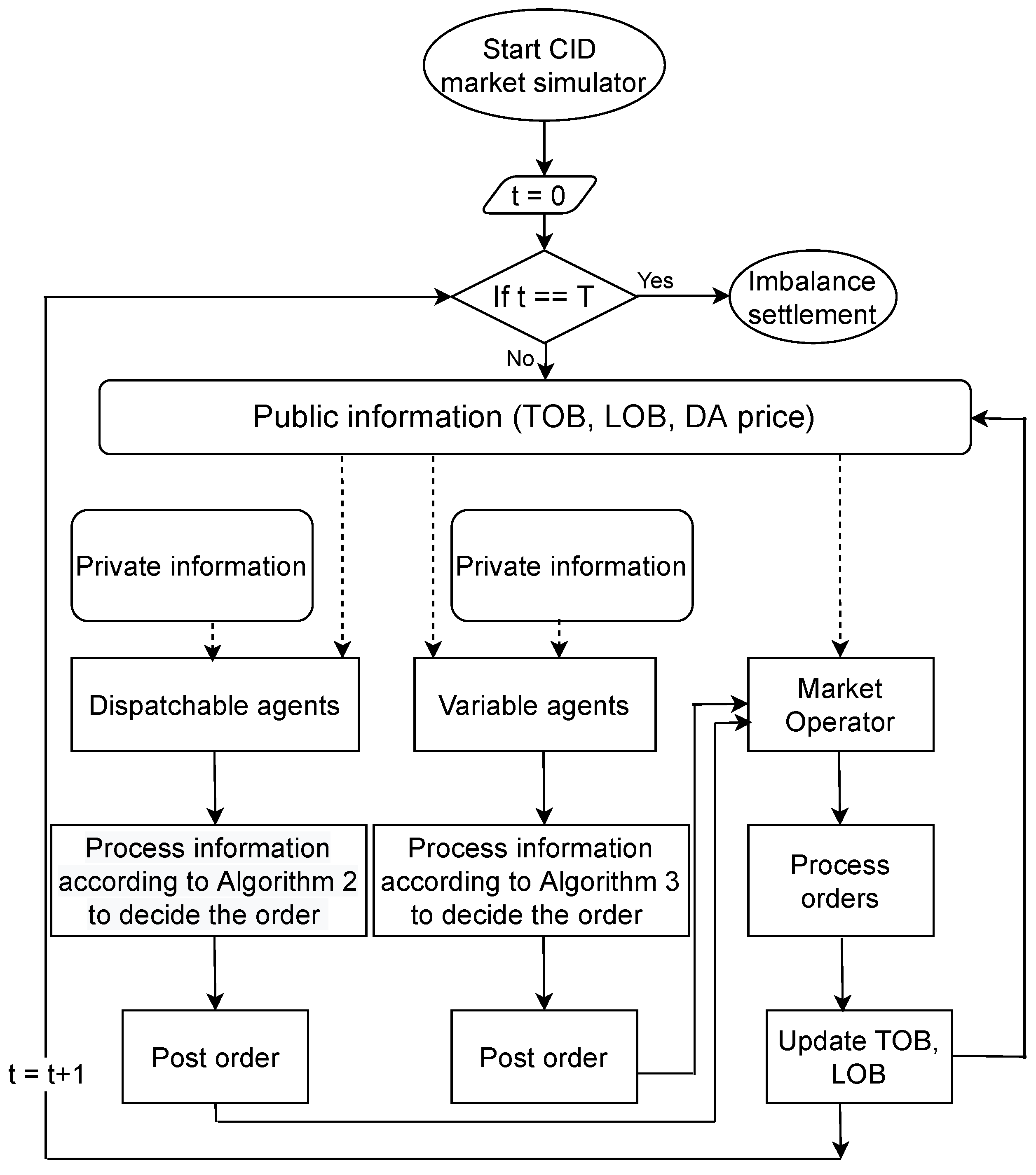
4.1. Continuous Market Operation

This subsection highlights the various steps taken consecutively by the MO agent to operate the continuous market clearing and the trading agents that submit their orders during the entire trading timeline. The market session is composed of a set of agents interacting over a discrete time horizon T. Let i denote an agent from the set I = { 1 , , N } where N is the number of agents. Additionally, let o b t denote the LOB at time-step t T .
Assumption 3.
A general assumption in this paper is that the only public information available to the trading agents is the top of the LOB t o b t and the DA price ( π D A ). The top of the LOB t o b t is a vector consisting of various price and volumes indicators: the best bid price b b p t , the best bid volume b b v t , the best ask price b a p t , the best ask volume b a v t , the volume weighted average price in the bid side v w a p b t and the volume weighted average price in the ask side v w a p a t . Compactly, we have:
t o b t = ( b b p t , b b v t , b a p t , b a v t , v w a p b t , v w a p a t ) .
At the beginning of the market session, the MO instantiates the LOB o b t o p e n . Then, at each time-step t, all the agents in the market are given a chance to post their orders. Each agent is assigned a unique identity number and the sequence in which these agents are selected to act is chosen randomly. Every agent, once selected by the MO, first cancels any of their previously submitted orders still in the order book o b t , and then submits a new order o i , t = ( y i , t , v i , t , π i , t ) according to their strategy S i . At this stage, the submitted order o i , t is processed by the MO and a new instance of the LOB emerges, i.e., o b t + 1 . The top of the LOB ( t o b t + 1 ) is also generated and shared among the agents for them to update their trading strategies. This process is repeated until the end of the trading horizon. The described process is presented in Algorithm 1. After CID trading, the imbalance settlement (detailed in Section 7) takes place, where deviations from the committed schedules are penalized.
Algorithm 1 Run the market
1:
procedureRunMarket( o b t o p e n )
2:
    for  t t o p e n , t c l o s e  do
3:
         i r a n d ( I )
4:
         o i , t S i ( t o b t )
5:
         o b t + 1 , t o b t + 1 MO Processing( o i , t , o b t , t o b t )
6:
        Update agents’ trading strategies
7:
    end for
8:
    Imbalance settlement
9:
end procedure

4.2. Order Processing

This subsection describes how the MO processes the orders submitted by the trading agents in the CID market. Once a new order o i , t is submitted by an agent, the MO determines whether a transaction is realized and updates the LOB accordingly. First, the MO checks the side of the order. For a buy (sell) order, the MO compares the price of the order ( π i , t ) with the best ask (best bid) price, and if π i , t is greater (lower) than the b a p t ( b b p t ), a transaction takes place. During this process, the matching volume v m a t c h and price π m a t c h are computed, as shown in the Appendix A. At this stage, an updated instance of the LOB o b t + 1 is generated. The orders whose entire volume is matched are removed from the LOB while the orders that are partially matched are first updated and then added to the LOB. The algorithms that compose the processing of the submitted orders can be found in Appendix A.

4.3. Updating Agents’ Beliefs

At each time-step t of the trading horizon, the MO communicates the top of the LOB (which is generated from the LOB o b t ) to the trading agents. With this information, the agents update their strategies S i as described in Section 5.1 and Section 6.

4.4. Transaction Confirmation

When a match takes place, the two parties of the transaction are notified and both of them locally confirm it, as described in Section 5.1.

5. Trading Agents

Two main types of trading agents are considered in the model, namely the dispatchable agents representing the operators of thermal power plants, and the variable agents representing renewable generators and consumers, among others. In this section, we first describe a generic agent that has all the common attributes and functionalities of the two aforementioned types of trading agents. Subsequently, the particular characteristics that differentiate them are elaborated.

5.1. Generic Agent

At each time-step t in the trading horizon, the information available to a trading agent can be divided, depending on its restriction level, into public and private.
Public information is considered to be available to all market participants at the same time and includes the top of the LOB t o b t and the day-ahead (DA) price π D A . On the other hand, the private information is only available to each individual agent. Formally, the public information available to an agent i in the current framework writes as
s i , t p u b l i c = ( t o b t , π D A ) .
In the following, a detailed description of the agents’ private information is introduced. Then, the modules that facilitate the interactions of the agent with the market environment are defined.

5.1.1. Private Information

The private information available to trading agent i contains the effective capacity C i , t of the production/consumption asset that can be traded at time-step t in the trading horizon. At the beginning of the trading horizon t o p e n , the effective capacity is defined as C i , t o p e n , and initialized with the value C i . The private information of an agent i also includes the market position p i , t m a r at time-step t, which represents the net volume of energy traded for the corresponding product. In particular, a positive (negative) market position indicates that the trading agent has sold (purchased) energy. At the beginning of the trading horizon, p i , t m a r is initialized with the value of the day-ahead market position, represented by p i d a . The private information also contains the cash-flow r i , t , which reflects the cumulative revenues of agent i during the trading process.
The difference between the market position p i , t m a r at time-step t and the expected energy output at physical delivery is denoted by imbalance δ i , t , which lists as additional private information for a given agent. The agent has private access to their most recent prediction for the positive and negative imbalance prices ( π ^ i , t i m b , + and π ^ i , t i m b , , respectively).
Assumption 4.
In this paper, it is assumed that all the trading agents aim to maximize their expected profits, taking into account payments for imbalances. The final imbalance Δ i is defined as the difference between the actual realization and the market position at the end of the trading horizon ( p i , t c l o s e m a r ). The trading decisions about the energy produced/consumed are such that the imbalance penalties are minimized.
During the trading process, an agent can be both a buyer and a seller. The minimum price an agent i is willing to offer and the maximum price they are willing to pay for a unit of power at time-step t are denoted by l i , t s e l l and l i , t b u y , respectively, and are considered additional private information. Finally, each agent maintains a local LOB o b i , t l o c a l during the trading process, as a private ledger tracking their outstanding orders at time-step t. This local LOB is updated when new orders are posted or when the existing (outstanding) ones are partially/fully accepted or canceled. Formally, the private information of an agent i writes as
s i , t p r i v a t e = ( C i , t , p i , t m a r , r i , t , δ i , t , π ^ i , t i m b , + , π ^ i , t i m b , , l i , t s e l l , l i , t b u y , o b i , t l o c a l ) .

5.1.2. Potential Functionalities

We define ‘potential functionality’ as a function that can be performed by a specific agent. In the case of a generic agent, the agent functionalities available are described as follows:

(1) Strategy S i ( t o b t )

This function comprises all necessary computations for submitting orders in the market. The definition and the interactions of this functionality with the rest of the simulator are detailed in Section 6. In its basic form, the pricing strategy receives as input the public information about t o b t . Based upon this, it computes all relevant information required for the design of the price–volume curves used for creating and submitting orders to the market.

(2) Outage O ( p o u t , c ˜ )

This function simulates the effect of receiving information regarding an unexpected outage within the available portfolio during the trading horizon. It takes as input an outage probability p o u t and the share of capacity which will be affected by the outage, given by c ˜ . The discrete event of an outage X { 0 , 1 } is sampled from a Bernoulli distribution defined as
P ( X | p o u t ) = ( p o u t ) X · ( 1 p o u t ) 1 X ,
where X = 1 corresponds to a capacity outage of share c ˜ . The outage functionality O is used to update the effective capacity C i , t at each time-step t by sampling a discrete event X t from Equation (2) and updating the effective capacity C i , t as in:
C i , t = ( 1 c ˜ ) · C , if X t = 1 C , otherwise .
Assumption 5.
In this paper, we assume that the up- and down-regulation prices are known to the market operator agent throughout the trading horizon. The other agents forecast these prices with some error. This assumption allows us to study the effect of information asymmetry of imbalance prices on the behavior of the agents.

(3) Imbalance Price forecaster I ( e i i m b )

This function is used to produce estimates of the imbalance prices π ^ i , t i m b , + , π ^ i , t i m b , of the traded product (time slot) at each time-step t. For the sake of simplicity, we assume that the imbalance price forecasts are given by adding white noise with variance e i i m b to the real positive and negative imbalance price denoted by π i m b , + , π i m b , , respectively. Thus, the imbalance prices are given by
π ^ i , t i m b , + = π i m b , + + N ( 0 , e i i m b )
π ^ i , t i m b , = π i m b , + N ( 0 , e i i m b )
Further details about the choice of π i m b , + and π i m b , are provided in Section 7.1.

(4) Confirm a Transaction Locally

This function enables a series of operations between parties in the case a transaction takes place between two agents at time-step t. First, the agents update their market position p i , t m a r and their cash-flow r i , t and then they update their local order book o b i , t l o c a l accordingly. For a transaction between two parties exchanging a volume of v m a t c h , at a price π m a t c h , the update of market positions and cash-flows for each party depending on their side y m a t c h , is given by
p i , t + 1 m a r = p i , t m a r + v m a t c h , if y m a t c h = S e l l v m a t c h , if y m a t c h = B u y
r i , t + 1 = r i , t + v m a t c h · π m a t c h , if y m a t c h = S e l l v m a t c h · π m a t c h , if y m a t c h = B u y
The local order book o b i , t l o c a l that contains all outstanding orders is updated after each transaction as follows. If the transacted volume v m a t c h fully matches the posted limit order volume v, the order is removed from the LOB. Otherwise, the order remains in the local book with an updated volume v i , t as reduced by v m a t c h .

5.2. Dispatchable Agent

This agent is built upon the previously described generic one and allows for the representation of trading agents controlling fully dispatchable assets, i.e., thermal plants.

5.2.1. Private Information

In addition to the private information of the generic agent, the dispatchable agent also tracks what we call buy and sell margins, g i , t d o w n and g i , t u p , respectively. At every time-step t, these margins correspond to the difference between the market position p i , t m a r and the minimum stable load C ̲ i , t (for a buy order) or the difference between the effective capacity C i , t and the market position p i , t m a r (for a sell order). Formally, these margins are given by
g i , t d o w n = max p i , t m a r min C ̲ i , t , C i , t , 0
g i , t u p = max C i , t p i , t m a r , 0
The private information of a dispatchable agent i writes as
s i , t p r i v a t e , d i s = ( s i , t p r i v a t e , g i , t d o w n , g i , t u p ) ,
where s i , t p r i v a t e is the private information available to the agent i at time t as per Equation (1) and g i , t d o w n and g i , t u p are the buy and sell margins according to the Equations (8) and (9), respectively.

5.2.2. Potential Functionalities

(1) Strategy S i , d i s ( t o b t )

Functionality is used to produce the order to be submitted to the market at time-step t, according to Algorithm 2. Firstly, agent i cancels all potential outstanding orders. Then, it computes the effective capacity C i , t according to Equations (2) and (3). The resulting capacity is used to compute the buy/sell margins according to Equations (8) and (9), respectively. Then, new imbalance prices forecasts ( π ^ i , t i m b , + and π ^ i , t i m b , ) are computed according to Equations (4) and (5) before the effective capacity C i , t is leveraged to evaluate the imbalance δ i , t as per:
δ i , t = min { C i , t p i , t m a r , 0 } + min { p i , t m a r C ̲ , 0 }
At the end of the trading horizon, the final imbalance Δ i for a dispatchable agent i is computed as Δ i = δ i , t c l o s e . In case the agent observes a negative imbalance δ i , t < 0 , the limit price buy l i , t b u y is updated. This happens as the agent prefers to buy the energy that cannot be physically produced via its unit than to face imbalance penalties. Again, this follows from Assumption 4 related to the requirement of the trading agents to be in balance at the real-time delivery stage. In such a situation, the updated limits are given by
l i , t + 1 b u y = ( 1 α ) l i , t b u y + α · max { π ^ i , t i m b , , l i , t o p e n b u y } , if δ i , t < 0 l i , t o p e n b u y , otherwise
l i , t s e l l = l i , t o p e n s e l l
It should be noted that the limit sell price l i , t s e l l remains the same for the entire trading session since the agent does not face any positive imbalance. In the final step, with all the public and private information available, agent i can use its pricing strategy P S i to produce the order o i , t that will be submitted to the market at time-step t.
Algorithm 2 Steps to decide the orders to be placed
1:
procedure S i , d i s ( t o b t )
2:
    Cancel outstanding orders
3:
    Update capacity( C i , t ) as per Equation (3)
4:
    Compute buy/sell margins g i , t d o w n , g i , t u p as per Equations (8) and (9)
5:
    Predict imbalance prices π ^ i , t i m b , + , π ^ i , t i m b , as per Equations (4) and (5)
6:
    Compute imbalance( δ i , t ) as per Equation (10)
7:
    Update limit price buy/sell l i , t b u y , l i , t s e l l as per Equations (11) and (12)
8:
     o i , t PS ( t o b t , s i , t p r i v a t e , d i s )
9:
    return  o i , t
10:
end procedure

5.3. Variable Agent

The variable agent is also built upon the previously described generic agent and contains additional attributes and functionalities that enable the representation of trading agents that control variable assets, i.e., renewable energy sources or consumption.

5.3.1. Private Information

Due to the variable nature of this type of agent, it is considered that the agent has access to a forecast p ^ i , t v a r at every time-step t, which is the most recent forecast of the uncertain production/consumption.
Assumption 6.
In this paper, we assume that the production/consumption forecast available to each agent is independent of other agents and does not consider any spatial correlation.

5.3.2. Potential Functionalities

(1) Forecasting functionality

Forecasts are produced by this functionality at a frequency D i , t , according to:
p ^ i , t v a r = F i ( C , e i , t c s t , p i , t v a r , p ^ i , 0 v a r ) ,
where C is the effective capacity as per Equation (3), e i , t c s t is the error constant, p i , t v a r and p ^ i , 0 v a r denotes the realization and initial forecast of the variable consumption/production, respectively. In this paper, we consider that the forecast of electricity consumption and RES production p ^ i , t v a r is generated by adding a systemic error e i , t v a r to the actual realization p i , t v a r , as per:
p ^ i , t v a r = p i , t v a r + e i , t v a r
The error e i , t v a r at time-step t is computed by one of the following functions:
  • Cosinusoidal forecast:
    e i , t v a r = C ˜ · cos t | T | 2 · e i , t c s t
  • Sinusoidal forecast:
    e i , t v a r = C ˜ · sin t | T | 2 · e i , t c s t
  • Constant offset forecast:
    e i , t v a r = C ˜
    where C ˜ denotes the amplitude/offset of the error and e i , t c s t is a constant that can adjust the frequency of the error. Thus, the private information of a variable agent i writes as
    s i , t p r i v a t e , v a r = ( s i , t p r i v a t e , p ^ i , t v a r ) .
    where s i , t p r i v a t e is the private information available to the agent i at time t according to Equation (1) and p ^ i , t v a r is the forecast of production/consumption of the variable agent.

(2) Strategy S i , v a r ( t o b t )

Functionality is used to produce the order to be submitted to the market at a decision time-step t, according to Algorithm 3. At first, agent i cancels all potential outstanding orders. Then, the agent computes an updated version of the effective capacity C i , t according to Equations (2) and (3) and receives the most recent forecast of consumption/production p ^ i , t v a r from Equation (13). Then, new imbalance price forecasts ( π ^ i , t i m b , + and π ^ i , t i m b , , respectively) are computed according to Equations (4) and (5). At each time-step t, the imbalance δ i , t of a variable agent is computed as the difference between their market position p i , t m a r and their most recent forecast p ^ i , t v a r as per:
δ i , t = p i , t m a r p ^ i , t v a r .
At the end of the trading horizon, the final imbalance Δ i for variable agent i is computed as
Δ i = p i , t m a r p i , t v a r .
If a variable agent has an imbalance δ i , t , they face the risk of being exposed to an imbalance penalty. To take this into account, the agent updates their limit buy/sell prices ( l i , t b u y , l i , t s e l l ) towards its estimates of the positive/negative imbalance prices ( π ^ i , t i m b , + , π ^ i , t i m b , ) according to:
l i , t + 1 b u y = ( 1 α ) l i , t b u y + α · max { π ^ i , t i m b , , l i , t o p e n b u y } , if δ i , t < 0 l i , t o p e n b u y , otherwise
l i , t + 1 s e l l = ( 1 α ) l i , t s e l l + α · min { π ^ i , t i m b , + , l i , t o p e n s e l l } , if δ i , t > 0 l i , t o p e n s e l l , otherwise
Finally, the variable agent i can use its pricing strategy P S i together with the available public and private information to produce an order o i , t that will be submitted to the market at time-step t.
Algorithm 3 Variable agent strategy
1:
procedure S i , v a r ( t o b t )
2:
    Cancel outstanding orders
3:
    Update capacity( C i , t ) as per Equation (3)
4:
    Compute recent forecast ( p ^ i , t v a r ) as per (13)
5:
    Predict imbalance prices π ^ i , t i m b , + , π ^ i , t i m b , as per Equations (4) and (5)
6:
    Compute imbalance( δ i , t ) as per Equation (17)
7:
    Update limit price buy/sell l i , t b u y , l i , t s e l l as per Equation (18)
8:
     o i , t PS ( t o b t , s i , t p r i v a t e , d i s )
9:
    return  o i , t
10:
end procedure

6. Pricing Strategies

As described in the previous section, after deciding the amount of energy to be put into the market, each agent i employs a pricing strategy P S i for this volume. More specifically, each agent needs to construct a price–volume curve that defines the price at which shares of the total volume will be placed into the market. In the following, the two available pricing strategies, namely a naive strategy and a modified trader AA strategy, will be described. In this section, first, a generic pricing scheme that serves as a basis for any of the two aforementioned strategies is introduced. Then, the naive and the modified trader AA pricing strategies are described in detail.

6.1. Generic Strategy

This strategy includes the common parameters and functions that any of the two proposed pricing schemes should contain in the current framework. Thus, irrespective of the pricing strategy, a set of parameters is required to construct the price–volume curve of an agent. This set includes (i) the updated values for the buy/sell limits ( l i , t s e l l , l i , t b u y ) (for the ease of notation, the index i will be dropped in the rest of this section as the concepts described here apply to each agent); (ii) the (user-defined) number of orders n that the agent submits to the market; and (iii) the top of the book at the previous time-step ( b b p t p r e v , b b v t p r e v , b a p t p r e v , b a v t p r e v ).
In addition, the generic pricing strategy is characterized by a set of processes. First, the agent initializes all relevant strategy parameters. Then, the agent learns the strategy parameters based on information received from the MO (e.g., top of the book, transactions). This update occurs at each market event and contains slightly different sub-processes depending on the pricing strategy in use. Finally, the agent constructs the price–volume curve and outputs the orders that are submitted to the MO.

6.2. Naive Strategy

This strategy builds the price–volume curve by randomly sampling from a range of prices. The additional parameters that are characteristic for the naive strategy are (i) the price range π r a n g e used for random sampling and (ii) the number of intervals m in which the price range is split. According to the naive strategy, an agent first initializes the values of l t s e l l , l t b u y , n, π r a n g e and m. Then, the values of the previous best bid/ask prices/volumes are updated according to the new top of the book received from the MO. Then, the agent passes the volume decision and the side of the orders to be posted and the price–volume curve is built. In the case that the agent attempts to sell a volume v, the naive strategy proceeds as follows. First, a price range is defined containing m intervals, with minimum and maximum values given by
π m i n s e l l = max { b b p t π r a n g e , l t s e l l }
π m a x s e l l = max { b a p t + π r a n g e , l t s e l l + π r a n g e }
Similarly, in the case the agent attempts to buy a volume v, the price range limits are given by
π m i n b u y = min { b b p t π r a n g e , l t b u y π r a n g e }
π m a x b u y = min { b a p t + π r a n g e , l t b u y }
The price step is defined as
Δ π = π m a x · π m i n · m
The sets containing the candidate prices for selling P s e l l and buying P b u y can be defined as
P s e l l = { π m i n s e l l , π m i n s e l l + Δ π , , π m a x s e l l }
P b u y = { π m i n b u y , π m i n b u y + Δ π , , π m a x b u y }
Then, a number of n price values π j , with j { 1 , . . , n } , are sampled i.i.d. from P s e l l or P b u y , while the volume v is shared equally among all orders (i.e., v 1 = . . . = v n = v n ). The final orders are defined as
o i , t = { ( π 1 , v 1 ) , ( π 2 , v 2 ) , , ( π n , v n ) }

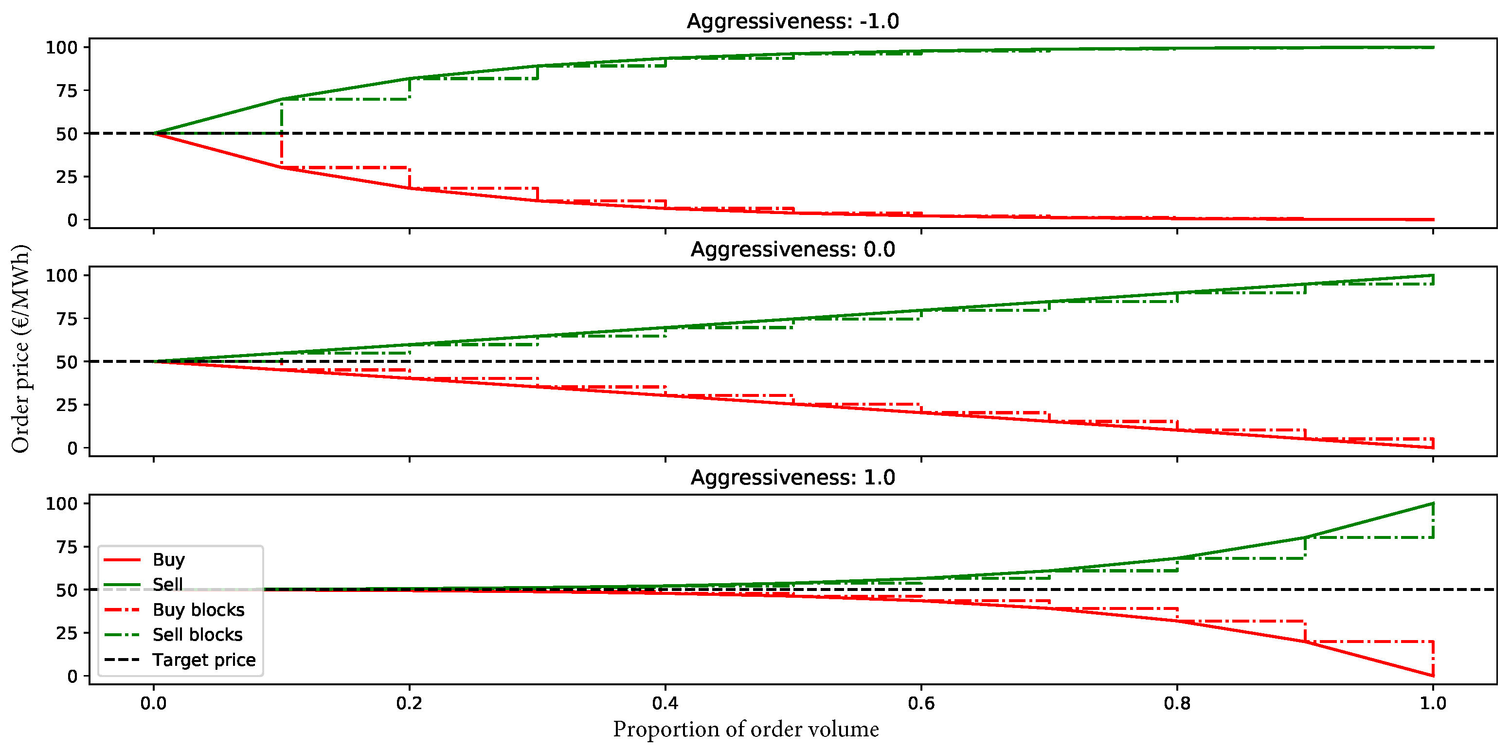
6.3. Modified Trader AA Strategy

This strategy builds the price–volume curve in two steps. First, the methodology introduced in the trader AA strategy, detailed by [35], is used to define the target price at each step. Subsequently, the target price is used as a reference point to build the price–volume curve. A first additional pricing strategy parameter that is specific to the MTAA scheme is the competitive equilibrium price estimate π ^ t . Second, the aggressiveness a t characterizes the trading behavior of an agent. It takes values in 1 , 1 , where a t > 0 corresponds to an aggressive trader (posting orders that are better than their π ^ t estimate), a t = 0 is associated with an active trader (posting orders that are at their estimate π ^ t ) and a t < 0 denotes a passive agent (posting orders that are worse than their estimate π ^ t ). A third MTAA parameter is the target price τ t that specifies the price that the agent is willing to offer given its aggressiveness level a t . In particular, the target price τ t is given by a parameterized exponential function with parameter θ .
The MTAA strategy implements the following steps. First, an initialization that retrieves the values of l t o p e n s e l l , l t o p e n b u y , n, π ^ t o p e n , a t o p e n and θ t o p e n from the agent occurs. This is followed by the learning of the parameters of the strategy after each time-step t, based on the received top of the order book and the transactions that might have taken place. The main parameters of the MTAA strategy are updated as follows:
  • The competitive equilibrium price estimate p ^ is computed at each step as the mean value of K past transactions according to:
    π ^ t = 1 K k = 1 K π k
  • The aggressiveness a is updated as
    a t + 1 = a t + β · ( δ p a t ) ,
    where δ p is a proxy of the degree of aggressiveness that would form a price equal to the best bid price b b p t , if the agent is a buyer and the last event is a bid, or equal to the best ask price, b a p t , if the agent is a seller and the last event is an ask. In case the last event is a transaction, the price reference is the transaction price π m a t c h . The learning process of the aggressiveness takes place in a step-wise manner that depends on the step-size parameter β .
  • The target price parameter θ is only updated when a transaction takes place, while the magnitude of the update depends on the market volatility ν through function θ ¯ ( ν ) . The updated parameters are given by
    θ t + 1 = θ t + β 1 · ( θ ¯ ( ν ) θ t ) ,
  • The target price τ t at each step t is computed as a function of the aggressiveness level a, the estimated equilibrium price π ^ t and the limit prices to buy/sell ( l t s e l l , l t b u y ). Compactly, it writes:
    τ t = g θ t ( l t s e l l , l t b u y , π ^ t , a t ) ,
    where θ t defines the shape of the exponential.
Finally, the last step involves learning the price–volume curve with the volume, decision, and side of the orders posted by the agent, the volume decision, and the side of the orders the agent will post and constructs the price–volume curve in a two-stage procedure. Building this curve is a two-step process. First, the decision on the bid/ask price is taken following the procedure described by [35]. More specifically, for determining the price at which a new order will be posted, the MTAA strategy uses the target price τ t and the observed top of the book t o b t . The price, depending on the side of the orders, is given by
π a s k = b a p t ( b a p t τ t ) / η
π b i d = b b p t + ( τ t b b p t ) / η
where η is a parameter that determines the rate of decrease (increase) in the ask price (bid price) and η [ 1 , ) . Then, given the resulting price and the agent aggressiveness, exponential price–volume curves for selling or buying energy are given by
P s e l l ( V ) = π a s k + ( π m a x π a s k ) · e V a t ϕ 1 e a t ϕ 1
P b u y ( V ) = π b i d + ( π m i n π b i d ) · e V a t ϕ 1 e a t ϕ 1
where V 0 , 1 represents the proportion of the volume v and π m a x , π m i n , ϕ are user-defined parameters that are used to define the price range of the curves.
Then, a number of n price values π j , with j { 1 , , n } , are derived from P s e l l ( V j ) or P b u y ( V j ) , where:
V j = l = 1 j v l v .
The volume v is shared equally among all orders (i.e., v 1 = = v n = v n ). The final orders are defined as
o i , t = { ( π 1 , v 1 ) , ( π 2 , v 2 ) , , ( π n , v n ) }
An illustration of the price–volume curves derived from MTAA strategy based on different aggressiveness values is shown in Figure 4.

7. Imbalance Settlement

The MO, in addition to running the ID market, is considered to be responsible for the final imbalance settlement after gate closure. This relies on the assumption that the final position of each agent at the gate closure is binding and the agent does not adjust its production/consumption during the physical delivery. The positive and negative imbalance prices ( π i m b , + and π i m b , , respectively) denote the penalties applied to positive and negative imbalances caused by the trading agents. The two prevailing imbalance mechanisms currently in use throughout Europe, namely single and dual pricing, are both available in the current framework, with the user being responsible to define which of the two is applied.
The single pricing mechanism applies a penalty to the agents that have a negative imbalance and remunerates the agents that have a positive one. The value of the imbalance prices under the single pricing mechanism is often the same based on the specific electricity market (i.e., π i m b , + π i m b , ) and depends on the sign and the size of the system imbalance. For instance, if the system imbalance is positive, a downwards regulation takes place. All imbalances are then settled at the downwards regulating price π d o w n and for the single pricing mechanism this implies π i m b , + = π i m b , = π d o w n . Formally, the single imbalance pricing settlement amount r i s i p , d o w n is given by
r i s i p , d o w n = π i m b , · Δ i .
Alternatively, when a negative system imbalance occurs, an upwards regulation takes place and imbalances are settled at the upwards regulating price π u p , which results in π i m b , + = π i m b , = π u p . In that case, the single imbalance pricing settlement amount r i s i p , u p will be:
r i s i p , u p = π i m b , + · Δ i .
The dual pricing mechanism applies a different price to the positive and the negative imbalances, respectively. For example, let R denote the regulation volume activated to counteract the system imbalance. In the case the system is in upwards regulation (i.e., negative system imbalance), an upward regulation price π u p is applied to the positive imbalances and the day-ahead price π D A is applied to the negative imbalances. Formally, π i m b , + = π u p and π i m b , = π D A . Thus, the dual imbalance pricing settlement amount under upwards system regulation (i.e., r i d i p , u p ) is given by
r i d i p , u p = π u p · Δ i , if Δ i > 0 π D A · Δ i , if Δ i < 0
In the case that the system is in downwards regulation (i.e., positive system imbalance), a downward regulation price π d o w n is applied to the negative imbalances and the spot price π D A is applied to the positive imbalances. Formally, π i m b , + = π D A and π i m b , = π d o w n . Hence, the dual imbalance pricing settlement amount under downwards system regulation (i.e., r i d i p , d o w n ) is given by
r i d i p , d o w n = π D A · Δ i , if Δ i > 0 π d o w n · Δ i , if Δ i < 0
If no regulation is activated, then all imbalances are treated at spot price π D A . As described above, the sign and the amount of the system imbalance (regulation sign) determine the penalty that will be attributed to the trading agents.

7.1. Impact on System Regulation

In this paper, we consider that the values for the upwards π u p and the downwards π d o w n regulation prices are predefined and do not depend on the regulation volume activated R. This way, the sign of the system regulation s g n ( R ) is sufficient to determine the imbalance prices ( π i m b , + and π i m b , , respectively), given the imbalance mechanism (single/dual pricing) considered and its computation proceeds as follows. First, a random variable Y { 0 , 1 } is sampled from a Bernoulli distribution that writes as
P ( Y | f ) = ( k ) Y · ( 1 k ) 1 Y ,
where k denotes the probability of having a positive imbalance. In order to incorporate the impact of the imbalances of trading agents in the imbalance settlement period (ISP), the imbalance influence factor f 0 , 1 is used. The cumulative imbalance caused by the trading agents is computed as
Δ m a r k e t = n N Δ i ,
while the probability k writes as
k = 0.5 + s g n ( Δ m a r k e t ) · f 2 .
On the one hand, when f = 0 , the sign of the imbalance Δ m a r k e t does not impact the system imbalance, which is then determined in a random way. On the other hand, if f = 1 , the cumulative imbalance of trading agents fully define the total system imbalance. Then, the sign of the system regulation R, given the realization of the random variable Y is given by
s g n ( R ) = + 1 , if Y = 0 1 , otherwise
Once the sign of the regulation volume is determined, the imbalance settlement takes place for each agent according to Equations (37)–(39).

8. Test Case, Results and Discussion

The presented ABM framework is used to evaluate three case studies based on a proposed market configuration. First, the impact of different pricing strategies on the market outcome is evaluated by gradually modifying the traders that adopt the MTAA strategy. Then, the effect of capacity outages in the market price formation process is validated. Finally, the effect of the imbalance price information asymmetry is analyzed.

8.1. Test Case Set-Up

In the following section, a case study with six trading agents is proposed. Among these, four are variable (two RES agents, W i n d 1 and W i n d 2 and two consumer agents, F l e x 1 and F l e x 2 ) and two are dispatchable ( T h e r 1 and T h e r 2 ), according to the classification in Section 5. Additionally, an MO agent is defined to manage and clear the orders submitted by the aforementioned traders.

8.1.1. Trading Agents Configuration

In line with Section 5, the trading agents have specific sets of input parameters. Numerical values for the listed parameters are presented in Table 1. The values in this table are set so as to maintain enough liquidity in the market in different case studies discussed in this section. For the variable agents, the forecast error drives their trading behavior and it is given by the difference between their updated forecasts and their updated position. At the gate-opening time of the CID market, the DA position is the initial position of the agents. The updated forecast is derived from the capacity and p v a r . For example, for the W i n d 1 agent, the updated forecast would be 2200 MWh, therefore, leading to a forecast error of 700 MWh from its initial DA position. The capacities, DA positions, and initial limit prices of the dispatchable agents are decided based on their characteristics to participate in the CID market if they can sell beyond their DA positions at a price above their marginal cost or buy at a low price in the CID market to produce less than their DA position. The forecasts of these agents are assumed to be updated every 5 min. The minimum stable load of the conventional agents is assumed to be 50 MW whereas the n o r d e r s value for all the agents are assumed to be equal to 10. Additionally, the input values of MTAA strategy parameters including β , η , and δ p are chosen according to [35].

8.1.2. Market Operator Configuration

In the current example, the MO processes orders for one single hourly product from 00:00 to 01:00 on day D, assuming a trading session that starts ( t o p e n H 1 ) at 16:00 and ends ( t c l o s e H 1 ) at 23:00 on day D 1 . The DA price is set to 30 EUR/MWh, while the upwards and downwards regulation prices are 160 EUR/MWh and 5 EUR/MWh, respectively. Dual imbalance pricing is adopted as imbalance settlement mechanism. Lastly, the time-step for the CID trade is considered to be 5 min.
The code for the simulations is written in Python 3.8. Simulations are performed on a GNU/Linux machine whose CPU is an Intel Core i7-8665U and with 16 GB of RAM. It takes 2 min to complete each simulation. The repository containing the proposed framework implementation as well as the test cases presented is freely accessible in GitLab [40].

8.2. Evaluating the Effect of Different Pricing Strategies

This subsection investigates the impact of the two available pricing strategies (i.e., naive and MTAA) on the agents’ revenues. To this end, four different simulations are run where the agents’ strategies are tested. In the first simulation (Wind AA), the RES agents adopt an MTAA strategy while the rest use a naive strategy. For the second simulation (Consumer AA), the consumer agents adopt an MTAA strategy, while the rests adopt the naive one. In the third simulation (Thermal AA), the conventional agents adopt the MTAA strategy, while the rest use a naive one. Finally, for the fourth simulation (All AA), all six agents adopt the MTAA pricing strategy.
In this case study, constant offset forecast (see Section 5.3 for details) is assumed to be adopted by all variable agents for the sake of simplicity. Based on the DA position of W i n d 1 and W i n d 2 and their generation forecast, they would predominantly act as sellers in the CID market. On the other hand, F l e x 1 and F l e x 2 would act as buyers in the CID market to be able to match their positions with their forecasts. T h e r 1 and T h e r 2 can either sell or buy in the CID market depending on whether they can be transacted at a lower price than their updated limit buy or higher price than their updated limit sell.
Table 2 lists the revenues (in k€) of all six agents after the ID gate closure (before the imbalance settlement stage) under different pricing strategies. The transaction prices in the CID market as a result of the strategies of the agents are shown in Figure 5.
Figure 5a displays the evolution of the transaction price in the Wind AA scenario. At the gate-opening of the CID market, the naive consumer agents ( F l e x 1 and F l e x 2 ) buy at their limit prices (150 EUR/MWh). Owing to high liquidity in the market during the initial few hours, they buy the deficit in their position and reach the forecasted consumption levels. W i n d 1 , W i n d 2 and T h e r 1 , T h e r 2 act as sellers to F l e x 1 , F l e x 2 until they reach their forecasted consumption. During these transactions, the F l e x 1 , F l e x 2 agents lower the prices of their bid orders according to the naive strategy. Consequently, the ask order prices for the MTAA agents are adapted to respond to the market. As F l e x 1 , F l e x 2 match their forecasts, the transaction price falls to 20 EUR/MWh. At this price level, around 18:20, the naive T h e r 1 , T h e r 2 agents start posting bid orders, as that price is equal to their limit to buy. The strategic W i n d 1 , W i n d 2 agents (the agents that follow the MTAA strategy are referred to as ‘strategic’ agents while those with the naive strategy are referred to as ‘naive’ agents) adapt to the prices in the market and are transacted until their positions become equal to their forecasts.
It can be observed from Figure 5b that when the F l e x 1 and F l e x 2 agents follow the MTAA strategy ( F l e x A A scenario), the transaction price at the CID gate opening is at 70 EUR/MWh, which is well below their limits to buy. Figure 5b and Figure 6b show how the strategic consumers can pay a lower price as compared to the scenarios ( W i n d A A and T h e r A A ) when they are naive while the producers are strategic. This explains why the cost incurred by the F l e x 1 and F l e x 2 agents in the CID market is lower in the F l e x A A scenario (61,260 EUR and 55,260 EUR) as compared to that in the W i n d A A scenario, as seen in Table 2. At the same time, it can be seen in Table 2 that the revenues earned by the naive wind agents (64,480 EUR and 61,760 EUR) for reaching the same final position (as seen from Figure 6a–c and Table 2) are reduced when F l e x agents are strategic.
The thermal agents in the CID market can sell above their limits to sell ( l s e l l ) and then buy at a cheaper price than what they have sold at as long as the price is below their limits to buy ( l b u y ). This behavior of the thermal agents can be observed in Figure 6a–c. Figure 6c shows the Thermal AA scenario where the thermal agents sell at a high price (above 150 EUR/MWh) at the gate opening of the CID market (16:00). They start buying from the naive wind agents 19:00 onwards. Following the MTAA strategy, both T h e r agents can transact. Moreover, the strategic T h e r agents trade their volumes in parts over a period of a few hours rather than trading the entire volume in a shorter time period as in Figure 6a,b. The effect of this can be seen on the revenues of the thermal agents in Table 2.
The time required for the transaction price to reach 20 EUR/MWh, which is the limit to buy for T h e r 2 , is different depending on the scenarios. In Figure 5a (Wind AA) where RES agents act as sellers while T h e r 1 and T h e r 2 are the buyers. It can be observed that the transactions take place at 20 EUR/MWh at 18:20. However, in Figure 5c (Thermal AA), the transaction prices reach 20 EUR/MWh at 19:00, when the sellers ( W i n d 1 and W i n d 2 ) are naive while the buyers ( T h e r 1 , T h e r 2 ) are strategic. Therefore, it can be inferred that if the sellers are strategic, the price can converge faster to the value at which the buyers can buy (limit to buy l b u y ). However, if the sellers are naive, this process of adaptation of the price to l b u y can be slower.
In Figure 5d, the transaction prices stay within the range of 61–69 EUR/MWh. In this case, all the agents follow the MTAA strategy. As the transaction price does not go below the limit to buy ( l b u y ) for the T h e r agents, they are not able to buy from the W i n d agents. As a result, W i n d 1 and W i n d 2 agents are only able to sell to the F l e x 1 and F l e x 2 agents, who have limited capacities to buy. The strategic F l e x 1 , F l e x 2 agents trade their volumes in parts over the entire trading horizon as opposed to the earlier cases. Therefore, the wind agents are not able to match their positions with their forecasts as opposed to the previous scenarios. This shows that the proportion of strategic agents and their capacities can have a significant effect on the transaction prices, thus influencing the liquidity and final positions of the agents in the CID market. As seen in Table 2, the revenues earned by wind and thermal agents are reduced, while costs incurred by Flex agents are less than the W i n d A A and T h e r A A scenarios.
Notably, the behavior of the variable agents in the CID market is sensitive to their DA positions and forecasts. The aim of the variable agents is to match their positions in the CID market to their updated forecasts. However, these agents are also limited by their capacities. Therefore, if the DA position of an agent is close to its capacity, it might reach its capacity limit soon and would not be able to trade further. This can give rise to lack of liquidity in the CID market, especially with a small number of trading agents. Hence, the effect of different price–volume strategies would become difficult to study in such type of a market setup.

8.3. Comparing the Response to Capacity Outages

As described in Section 5, the agents can update their preferences in the wake of an extreme event, e.g., an outage. This subsection analyzes the effect of information of an outage event on the behavior of the agents and the transaction prices. As the strategy followed by each agent is responsible for deciding its behavior, the effect of the information of outages is studied and compared when the agents follow either an MTAA or a naive strategy. The following cases describe the different strategies followed by the agents.
  • Case I: all the agents follow the naive strategy;
  • Case II: only the agent that suffers the outage follows an MTAA strategy while all the other agents are naive;
  • Case III: all agents adopt the MTAA strategy except the one that suffers the outage;
  • Case IV: all agents follow the MTAA strategy.
To showcase the impact of outages on the behavior of agents, a series of experiments are conducted. First, the effect of receiving information about an outage for T h e r 1 at different time instants in the trading session is simulated, and the associated results are centralized in Table 3. Then, similarly, the effect of knowledge of 100% outage in the portfolio of W i n d 1 at different time instants is evaluated. The corresponding results from W i n d 1 outage simulations are summarized in Table 4.
In Table 3, it can be seen that the response to the outage of T h e r 1 is highly sensitive to the strategies adopted by T h e r 1 and the other agents. It also depends on the time when the outage takes place. Consider Case II ( T h e r m a l A A ) when the outage is received at 75% of the trading horizon, a substantial price increase of 325% is observed. As the outage takes place closer to the gate-closure, the less expensive agents ( W i n d 1 and W i n d 2 ) have already reached their forecasted set points and do not sell to the T h e r 1 agent. Therefore, a more expensive naive T h e r 2 whose limit to sell is above 80 EUR/MWh is activated in the market, setting the prices to 85 EUR/MWh.
In Case II ( T h e r m a l A A ), the naive agents lead the prices in the market and the MTAA agent follows. A similar principle also applies to Case III when only the unit with an outage is naive but the others are strategic. The relative change in transaction prices is significant in Case III as the T h e r 1 agent is naive and other agents are strategic.
In Case IV, when all the agents follow an MTAA strategy, the agents trade the volume in parts throughout the trading horizon and the transaction prices are generally higher as compared to the other cases. In this case, if an outage of T h e r 1 is going to happen, then the relative change in prices is not that significant as the agents learn slowly per the market event (outage). As a result, the unit that will suffer the outage is still able to buy back in the CID market but in small parts of volume distributed over several hours until gate closure. Trading smaller volumes with time leads to smaller price change rather than a surge in price if the entire volume was being traded in a short duration of time—therefore, avoiding a sudden surge in prices.
It can be seen that there is a less significant relative increase in price when the outage occurs at the beginning of the trading horizon (t = 25%) as compared to near the gate closure (t = 75%). One of the main reasons for this difference can be that the transaction prices are already higher in the market at the beginning. Therefore, a further increase in price does not create a spike in price.
A common observation from Table 3 and Table 4 shows that there is always an increase in price when producers T h e r 1 and W i n d 1 are informed about the outages. There is a difference between the relative changes in prices in Table 3 and Table 4 for outages of the thermal and wind producers, respectively. These differences are owed to the fact that the limit to buy ( l b u y ) for the wind agent is higher than the thermal agents. Therefore, under certain circumstances, when the unit that loses the capacity needs to buy, it can pay a high price depending on its limit to buy, thus increasing the prices in the market.

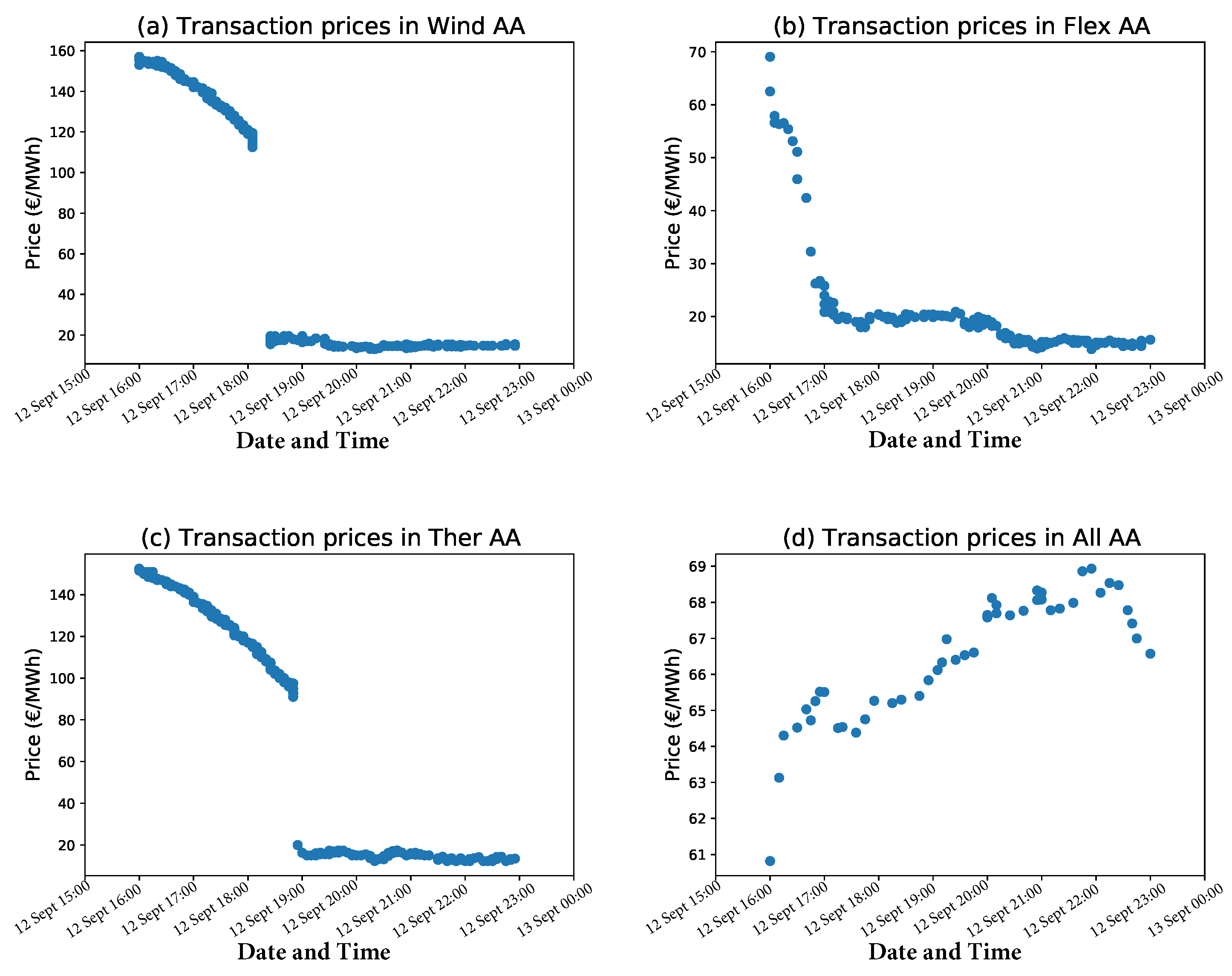
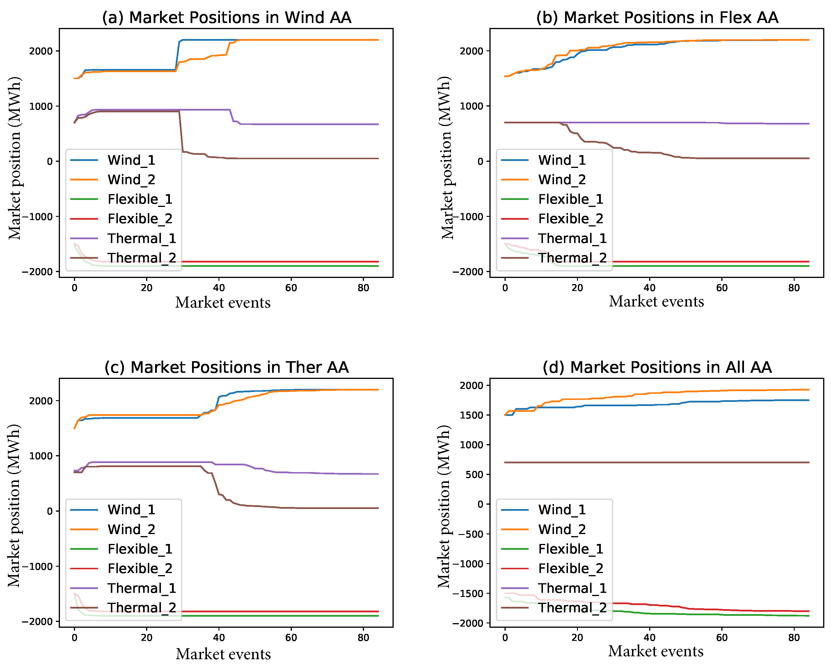
8.4. Evaluating the Effect of the Imbalance Price Information Asymmetry

In an electricity market, some agents have better estimates of the imbalance prices as compared to others. Based on the estimates of imbalance prices available to each variable agent, they may either prefer to remain in imbalance or trade in the CID market to reach its forecasted generation or consumption. This subsection discusses the effect of information asymmetry on the behavior of the agents in the CID market (in this study, in relation to information asymmetry, all the agents are assumed to follow the MTAA stategy). According to Equations (4) and (5), the estimates of imbalance prices can be varied by assigning different values to e i m b .

8.4.1. Effect of Information Asymmetry on the Wind Agent

In this case study, we analyze the effect of information asymmetry on W i n d 1 agent. To perform the analysis, we make certain assumptions about the values of white noise variance ( e i m b ). The estimates of the imbalance price values to the agents is obtained by adding the real imbalance prices ( π ^ i , t i m b , + , π ^ i , t i m b , ) to the variance generated by e i m b , the detailed expression is provided in Section 5.1. In this analysis, we keep the value of e i m b equal to zero for all other five agents but W i n d 1 and vary e i m b for the latter. The input data used for this study are similar to those in Table 1; however, a few parameters, namely the limit to sell ( l s e l l ) for W i n d 1 and W i n d 2 and realization ( p v a r ) value for W i n d 1 , were modified. The l s e l l for W i n d 1 and W i n d 2 agents was set to 30 EUR/MWh while p v a r value for W i n d 1 was set to 2000 MWh.
The value of e i m b is increased from 50 EUR/MWh to 250 EUR/MWh, thus making the estimate of imbalance prices worse for the W i n d 1 agent. The estimate of imbalance prices affects the limits set by the agent according to Equation (19). The W i n d 1 agent remains in positive imbalance throughout the trading horizon. Therefore, it is interesting to observe the change in the limit to sell ( l s e l l ) of W i n d 1 with the change in e i m b . The W i n d 1 agent compares its performance with the imbalance settlement. As e i m b is increased, the W i n d 1 agent starts underestimating the value of the down-regulation price. Therefore, the W i n d 1 agent lowers its limit to sell to transact and reach its forecasted generation rather than staying in imbalance. The W i n d 1 agent would otherwise be paid in the imbalance settlement stage according to its low estimate of down-regulation price.
Table 5 shows the relative change in transaction prices for different values of e i m b . With the increase in e i m b , the information about imbalance prices is made worse. As a result, the limit to sell for the W i n d 1 agent fluctuates more for a larger value of e i m b . On the other hand, the W i n d 2 agent has perfect information of the imbalance prices with e i m b = 0 , therefore, at the beginning of the trading horizon, it sets its limit to sell to 5 EUR/MWh, which is the actual value of the down-regulation price. The W i n d 2 agent does not change its limit to sell after that due to perfect information about the down-regulation price. It can be seen in the second row of Table 5 that the transaction price at the gate opening of the CID market, ( π t r o p e n ), takes a value around 80 EUR/MWh. However, the way the transaction prices evolve during the trading horizon changes with the values of e i m b . The transaction price at the gate closure ( π t r c l o s e ) as seen in Table 5 is different based on the values of e i m b .

8.4.2. Effect of Information Asymmetry on the Flexible Agent

To study the effect of information asymmetry from a buyer’s standpoint, the e i m b value for F l e x 1 is increased from 0 to 300 EUR/MWh, while that of the other five agents is kept at 0 EUR/MWh. During this analysis, the limit to sell ( l s e l l ) for W i n d 1 and W i n d 2 agents was set to be 30 EUR/MWh. The realization ( p v a r ) value for W i n d 1 was set at 2000 MWh. The value of limit to buy ( l b u y ) for F l e x 1 and F l e x 2 agents was made equal to 70 EUR/MWh.
The effect of variation of e i m b of F l e x 1 agent on the transaction price can be seen in Table 6. This table shows how the value of e i m b of F l e x 1 agent affects the transaction prices. With the increase in the error of the imbalance price estimate for the F l e x 1 agent, it erroneously overestimates the positive imbalance price ( π ^ i , t i m b , + ). As a result, according to Equation (18), the agent updates its limit to buy ( l i , t b u y ) according to the new estimate of π ^ i , t i m b , + , which is greater than its previous value. This leads to an increase in the l i , t b u y of the F l e x 1 agent, which results in elevated order prices posted by the agent. Therefore, an increment in the transaction price in the CID market with time is observed.
The effect of e i m b on the limit to buy ( l b u y ) or sell ( l s e l l ) depends on the initial limits of the variable agent of interest and that of other agents in the market. For example, if we are studying the effect of information asymmetry on a buyer and if its limit to buy is above the limit to sell of potential sellers, then the e i m b variation does not make any difference to the transaction prices or the way the limit to buy adapts. In such a case, the initial limit to buy for buyers needs to be set at a lower value than the limit to sell, and then as the e i m b value is increased, the limit to buy increases to be transacted in the CID market. This study on the information asymmetry of imbalance prices shows the importance of publishing the information about balancing reserves activated by the system operators in real time. The lack of this would cause information asymmetry, which can favor a few market participants who can then influence the market price.

8.5. Discussion

In this section, we discuss the limitations of the presented framework and the developed pricing strategies. More specifically, one central assumption is that we have discretized the CID market timeline so that the agents are allowed to submit orders at equidistant time instants. However, in reality, the trade can take place at any time in the trading horizon. This may lead to different outcomes when large time-steps are considered. In addition, the agent configuration selected for each experiment is critical and should be carefully selected to reflect a realistic market instance. The behavior of the agents in the CID market is sensitive to their DA positions, capacities, and forecasts. If the DA position input of an agent is close to its capacity, it might soon reach its capacity limit in the CID market trading horizon and would not be willing to trade further. This can give rise to a lack of liquidity in the CID market, especially with a few numbers of trading agents. Hence, in such a market setup, the effect of different price–volume strategies would become difficult to assess. With the availability of sufficient data, a realistic market configuration can be tested with the proposed ABM to derive more practical insights.
In addition, in this paper, we assume that the strategic variables of each agent are not public, and consequently, the rest of the agents do not have access to any of this information. However, in a real market setting, there might be universally available forecasts of wind, solar, or electricity load, which could directly facilitate the predictions of the other agent strategies or future prices. However, to simplify the simulation process, we consider that the agents do not have access to this information. The MTAA pricing strategy allows for the agents to decide their order prices by considering the past transaction prices in the market and the submitted orders. The order prices can then be updated each time the agent submits an order in the CID market. In the naive strategy, the agents have no access to the past or future values of the prices.

9. Conclusions

In this paper, we proposed an agent-based modeling framework to simulate the behavior and interaction of different agents in the European CID market. In particular, dispatchable as well as variable agents can trade electricity through a centralized limit order book, which is constantly updated by the electricity market operator. Two pricing strategies are considered according to which the trading agents can decide upon the orders to be posted in the CID market, namely a naive and a learning-based adaptive aggressiveness (AA) trading strategy. The proposed adaptive trading strategy was found to perform better than the naive strategy in terms of the revenues accumulated by the agents in the CID market. The proportion of strategic agents in the CID market was found to have a significant effect on the transaction prices, thus influencing the liquidity and final positions of the agents in the CID market. The strategic producers were able to exploit the limit prices of the naive consumer agents in the market, leading to high transaction prices in the market.
Furthermore, this paper shows that, in the case of an outage of a dispatchable agent, the prices in the market increase, and the surge in price is larger as the outage takes place closer to the gate closure. A more significant change in prices takes place when a strategic agent suffers an outage while other agents are naive, and in the case that a naive agent suffers an outage while others are strategic. However, when all the agents are strategic a substantial price increase is not observed. Therefore, in the wake of an outage, it is beneficial if the agents adopt the proposed learning-based strategy to avoid the high transaction prices. We further show that, in the case of information asymmetry in the imbalance prices, there is a decrease/increase in the limit to sell/buy of the agents, therefore leading to a decrease/increase in the transaction prices. Therefore, the revenues (cost) earned by sellers (buyers) are reduced (increased) as an effect of information asymmetry.
The key findings of this paper can be summarized as follows:
  • The proposed ABM provides a formalized tool to study the behavior of agents (market players) under different CID market settings;
  • The MTAA strategy presented in this work outperforms the benchmark (i.e., a naive strategy) in terms of revenue and coping after outages;
  • Information asymmetry among agents regarding the imbalance prices influences the transaction prices in the CID market, favoring those agents with more information.
Future work could be directed towards modeling hydro-power, energy storage and other agents in the CID market. An extension of the framework to include multiple products is another interesting addition to the existing agent-based model. Effort could be put in the future to add transmission constraints and perform larger case studies.

Author Contributions

Conceptualization, P.S. and I.B.; methodology, P.S. and I.B.; software, P.S. and I.B.; formal analysis, P.S. and I.B.; investigation, P.S.; data curation, P.S.; validation, P.S., I.B., D.R., and M.M.d.V.; writing—original draft preparation, P.S.; writing—review and editing, I.B., D.R., M.M.d.V., and M.A.; visualization, P.S.; supervision, M.A.; project administration, P.S.; funding acquisition, M.A. All authors have read and agreed to the published version of the manuscript.

Funding

This research was funded by the Swedish Energy Agency.

Institutional Review Board Statement

Not applicable.

Informed Consent Statement

Not applicable.

Data Availability Statement

All data utilized in the case studies is provided in the Section 8, ‘Test Case, Results and Discussion’.

Acknowledgments

The authors are thankful to the Swedish Energy Agency for the financial support to carry out this research work.

Conflicts of Interest

The authors declare no conflict of interest.

Nomenclature

The following abbreviations are used in this manuscript:
Abbreviations
A A Adaptive aggressiveness
A B M Agent-based model
C D A Continuous double auction
C I D Continuous intra-day
D A Day ahead
F C F S First-come–first-serve
I D Intra-day
I S P Imbalance settlement period
L O B Limit order book
M O Market operator
M T A A Modified trader adaptive aggressiveness
R E S Renewable energy sources
T O B Top of the order book
W P P Wind power producer
X B I D Cross-border intra-day
The main notation is presented below for a quick reference. Additional symbols are introduced throughout the text.
Indices
iAgent that participates in the CID market
tTime
j Order number
Parameters
t o p e n H 1 Gate opening time for intra-day trade for hourly product H 1
t c l o s e H 1 Gate closing time for intra-day trade for hourly product 1 H
t d e l i v e r y H 1 Start time of the physical delivery for hourly product H 1
t s e t t l e H 1 End time of the physical delivery for hourly product 1 H
T ˜ CID trading horizon for a specific CID product
Δ t Discretization step for the trading horizon
NTotal number of agents participating in the CID market
π D A Day-ahead price
p i d a Position of an agent i after DA market clearing
C i , t o p e n Effective capacity of agent i at time t o p e n
nNumber of orders placed by an agent in CID market
e i i m b Factor to represent the deviation of the forecast with respect tothe real
imbalance price
π i m b , + Real positive imbalance price
π i m b , Real negative imbalance price
π u p Up-regulation price
π d o w n Down-regulation price
C ̲ i Minimum stable load of a dispatchable agent i
α A step factor to update limit prices
l i , 0 b u y Initial limit of an agent to buy
l i , 0 s e l l Initial limit of an agent to sell
C ˜ Amplitude/offset of the forecast error
e i , t c s t Parameter to define the shape of forecast of agent i at time t
D i , t Frequency of arrival of new forecasts
p i v a r The actual production/consumption of a variable agent
RParameter indicating the size and sign of regulation volume to counteract
the system imbalance
kProbability of having a positive imbalance
fImbalance influence factor
Variables
Binary Variables
YBinary variable that indicates if the system was up- or down-regulating
y i , t Order side of an order posted by agent i at time t
Positive Variables
g i , t d o w n The volume that a dispatchable agent i can buy at t
g i , t u p The volume that a dispatchable agent i can sell at t
C i , t Effective capacity of an agent i at time t
v i , t Volume of an order posted by agent i at time t
v i , t r e m Remainder volume from order i at time t
v i , t m a t c h Matched volume from order i at time t
b b v t Best bid volume at time t
b a v t Best ask volume at time t
v m a t c h Volumes matched in a transaction
Continuous Variables
r i , t Cumulative revenues collected by an agent i at each time-step t of the
trading process
π i , t Price of an order posted by agent i at time t
b b p t Best buy price at time t
b a p t Best ask price at time t
v w a p b t Volume weighted-average price in the bid side at t
v w a p a t Volume weighted-average price in the ask side at t
π m a t c h Price at which orders are matched
p i , t m a r The net volume of energy traded by agent i until time-step t
δ i , t Imbalance of an agent i at time t
π ^ i , t i m b , Recent prediction of negative imbalance price by agent i at time t
π ^ i , t i m b , + Recent prediction of positive imbalance price by agent i at time t
Δ i Final imbalance of an agent i
l i , t b u y Maximum price that an agent i is willing to pay to buy at time t
l i , t s e l l Minimum price at which an agent i can sell at time t
p i , t m a r The market position at the closing time of the CID market
p ^ i , t v a r The recent forecast of uncertain production/consumption at t
e t v a r Error component that relates the forecasted and actual production/
consumption of variable agents
b b p t p r e v Best bid price of the previous step
b a p t p r e v Best ask price of the previous step
b b v t p r e v Best bid volume of the previous step
b a v t p r e v Best ask volume of the previous step
r n s i p Single imbalance pricing settlement amount
r n d i p , u p Dual imbalance pricing amount under up-regulation
r n d i p , d o w n Dual imbalance pricing amount under down-regulation
Δ m a r k e t The cumulative imbalance caused by agents trading in the CID market
Compilation of Variables
o b t Order book that contains outstanding bids and asks at time t
o i , t Order posted by an agent i at time t
t o b t Top of the order book at time t
Sets
ISet of agents participating in the CID market
TSet of time-steps available for trading in CID market
P s e l l Set of candidate prices in naive strategy
o b i , t l o c a l A private ledger by agent i to track its outstanding orders in the CID
market at time-step t
s i , t p r i v a t e Set of private information available to agent i at time t
s i , t p r i v a t e , d i s Set of private information available to a dispatchable agent i at time t
Outage Parameters
p o u t Probability of outage
c ˜ Outage percentage
Naive Strategy Parameters and Variables
π r a n g e Size of price range considered in naive strategy
mThe number of evenly spaced parts of price range in naive strategy
π m i n b u y Minimum price value at which a naive agent can buy
π m a x b u y Maximum price value for a naive agent to buy
π m i n s e l l Minimum price value at which a naive agent can sell
π m a x s e l l Maximum price value for a naive agent to sell
P s e l l Set containing the candidate prices for ask orders
P b u y Set containing the candidate prices for bid orders
Δ π Price step
MTAA Strategy Parameters and Variables
π m i n User-defined minimum price value for MTAA strategy
π m a x User-defined maximum price in the MTAA strategy
π i , t a s k Price of an ask order determined by MTAA strategy for agent i at time t
π i , t b i d Price of a bid order determined by MTAA strategy for agent i at time t
a i Aggressiveness of agent i
τ i Target price for an agent i
θ Parameter that relates r with τ
π ^ Competitive equilibrium price
β Step-size parameter to update aggressiveness
ν Market volatility
P s e l l ( V j ) Set of price values of ask orders as a function of proportion of order volume
P b u y ( V j ) Set of price values of bid orders as a function of proportion of order volume
Operators
m a x Maximum operator
m i n Minimum operator

Appendix A. Algorithms

Algorithm A1 Order processing
1:
function Process( o i , t , o b t , t o b t )
2:
     if  y i , t = B I D  then
3:
         if  π i , t b a p t  then
4:
             v r e s v i , t
5:
             v m a t c h Match( v r e s , y i , t , b a v t )
6:
             π m a t c h b a p t
7:
             o b t + 1 , t o b t + 1 Update LOB( o b t , v m a t c h )
8:
             o i , t Update order( v r e s )
9:
            Go to line 3
10:
        else
11:
            o b t + 1 o b t . A D D ( o i , t )
12:
        end if
13:
    else
14:
        if  π i , t b b p t  then
15:
            v r e s v i , t
16:
            v m a t c h Match( v r e s , y i , t , b b v t )
17:
            π m a t c h b b p t
18:
            o b t + 1 , t o b t + 1 Update LOB( o b t , v m a t c h )
19:
            o i , t Update order( v r e s )
20:
           Go to line 14
21:
        else
22:
            o b t + 1 o b t . A D D ( o i , t )
23:
        end if
24:
    end if
25:
    return  o b t + 1 , t o b t + 1
26:
end function
Algorithm A2 Match
1:
functionMatch( v r e s , y i , t , v t )
2:
     if  y i = B I D  then
3:
         while  v r e s > 0  do
4:
         end while
5:
         if  v r e s > v t  then
6:
             v m a t c h = v r e s v t
7:
         else
8:
             v m a t c h = v r e s
9:
          end if
10:
    else
11:
        while v r e s > 0
12:
        if  v r e s > v t  then
13:
            v m a t c h = v r e s v t
14:
        else
15:
            v m a t c h = v r e s
16:
        end if
17:
    end if
18:
    return  v m a t c h
19:
end function
Algorithm A3 Update LOB
1:
functionUpdate ob( o b t , v m a t c h )
2:
     if trade = TRUE then
3:
         if  y i = B I D  then
4:
            if  v r e s > b a v t  then
5:
                 A D D ( o t ) and R E M O V E ( o b a v t )
6:
            else if  v r e s = b a v t  then
7:
                 R E M O V E ( o b a v t )
8:
            else
9:
                 M O D I F Y ( o b a v t )
10:
           end if
11:
        else
12:
           if  v r e s > b b v t  then
13:
                A D D ( o t ) and R E M O V E ( o b b v t )
14:
           else if  v r e s = b b v t  then
15:
                R E M O V E ( o b b v t )
16:
           else
17:
                M O D I F Y ( o b b v t )
18:
           end if
19:
        end if
20:
    else
21:
         A D D ( o t )
22:
    end if
23:
    return  o b t + 1 , t o b t + 1
24:
end function
Algorithm A4 Update posted order
1:
functionUpdate order( o b )
2:
     v t + 1 r e s v t m a t c h v t r e s
3:
end function

References

  1. ENTSOE. Power Facts Europe 2019. Available online: https://eepublicdownloads.blob.core.windows.net/public-cdn-container/clean-documents/Publications/ENTSO-E%20general%20publications/ENTSO-E_PowerFacts_2019.pdf (accessed on 8 March 2021).
  2. Neuhoff, K.; Ritter, N.; Salah-Abou-El-Enien, A.; Vassilopoulos, P. Intraday Markets for Power: Discretizing the Continuous Trading? 2016. Available online: https://ssrn.com/abstract=2723902 (accessed on 25 June 2021).
  3. Ciferri, D.; D’Errico, M.C.; Polinori, P. Integration and convergence in European electricity markets. Econ. Politica 2020, 37, 463–492. [Google Scholar] [CrossRef] [Green Version]
  4. Pogosjan, D.; Winberg, J. Förändringar av Marknadsdesign och deras påverkan på balanshållningen i det Svenska Kraftsystemet: En kartläggning och analys av de Balansansvarigas arbetsgång. 2013. Available online: https://www.svk.se/siteassets/5.jobba-har/dokument-exjobb/forandringar-av-marknadsdesign-och-deras-paverkan-balanshallningen.pdf?_t_id=qWowEhUA1rBRRNtzXdqH-w==&_t_uuid=-UEFAhWSR7eX49e5YldH_Q&_t_q=sf6-gas&_t_tags=language:sv,siteid:40c776fe-7e5c-4838-841c-63d91e5a03c9,andquerymatch&_t_hit.id=SVK_WebUI_Models_Media_OfficeDocument/_ffc3ccaf-a4bd-441d-a665-a05a3e9b59d8&_t_hit.pos=259 (accessed on 15 February 2021).
  5. Dobschinski, J.; De Pascalis, E.; Wessel, A.; von Bremen, L.; Lange, B.; Rohrig, K.; Saint-Drenan, Y.M.; Fraunhofer, I.W.E.S.; ForWind, O.; Germany, E. The potential of advanced shortest-term forecasts and dynamic prediction intervals for reducing the wind power induced reserve requirements. In Proceedings of the Scientific Proceedings of the European Wind Power Conference, Warsaw, Poland, 20–23 April 2010; pp. 177–182. [Google Scholar]
  6. Holttinen, H. Handling of wind power forecast errors in the nordic power market. In Proceedings of the Probabilistic Methods Applied to Power Systems, Stockholm, Sweden, 11–15 June 2006. [Google Scholar]
  7. Le, H.L.; Ilea, V.; Bovo, C. Integrated European intra-day electricity market: Rules, modeling and analysis. Appl. Energy 2019, 238, 258–273. [Google Scholar] [CrossRef]
  8. Schittekatte, T.; Reif, V.; Meeus, L. The EU Electricity Network Codes (2019 ed.). Available online: https://fsrglobalforum.eu/wp-content/uploads/2019/03/FSR_2019_EU_Electricity_Network_Codes.pdf (accessed on 21 February 2021).
  9. Nordic TSOs. Short-Term Markets. Available online: https://www.svk.se/siteassets/press-och-nyheter/nyheter/tsos-discussion-paper-for-consultation.pdf (accessed on 4 December 2020).
  10. Coulter, K. 5 Trends Reshaping Today’s Global Power Market. Available online: https://www.renewableenergyworld.com/2020/01/14/5-trends-reshaping-todays-global-power-market/#gref (accessed on 12 March 2021).
  11. Nord Pool. Bots Disguised as Electricity Traders Are Placing Orders. Available online: https://careers.nordpoolgroup.com/blog/posts/25998-bots-disguised-as-electricity-traders-are-placing-orders (accessed on 5 April 2021).
  12. NordPool. Nord Pool Key Statistic July 2019. Available online: https://www.nordpoolgroup.com/message-center-container/newsroom/\exchange-message-list/2019/q3/nord-pool-key-statistics—july-2019/ (accessed on 10 December 2020).
  13. Shinde, P.; Amelin, M. A literature review of intraday electricity markets and prices. In Proceedings of the 2019 IEEE Milan PowerTech, Milan, Italy, 23–27 June 2019; pp. 1–6. [Google Scholar]
  14. Skajaa, A.; Edlund, K.; Morales, J.M. Intraday trading of wind energy. IEEE Trans. Power Syst. 2015, 30, 3181–3189. [Google Scholar] [CrossRef] [Green Version]
  15. Boukas, I.; Ernst, D.; Théate, T.; Bolland, A.; Huynen, A.; Buchwald, M.; Wynants, C.; Cornélusse, B. A deep reinforcement learning framework for continuous intraday market bidding. arXiv 2020, arXiv:2004.05940. [Google Scholar]
  16. Richard Scharff and Mikael Amelin. Trading behaviour on the continuous intraday market elbas. Energy Policy 2016, 88, 544–557. [Google Scholar] [CrossRef]
  17. Alexander von Selasinsky. The Integration of Renewable Energy Sources in Continuos Intraday Markets for Electricity. Ph.D. Thesis, TU Dresden, Dresden, Germany, 2016.
  18. Vytelingum, P. The Structure and Behaviour of the Continuous Double Auction. Ph.D. Thesis, University of Southampton, Southampton, UK, 2006. [Google Scholar]
  19. Veselka, T.; Boyd, G.; Conzelmann, G.; Koritarov, V.; Macal, C.; North, M.; Schoepfle, B.; Thimmapuram, P. Simulating the Behavior of Electricity Markets with an Agent-Based Methodology: The Electric Market Complex Adaptive Systems (emcas) Model; Center for Energy, Environmental, and Economic Systems Analysis (CEEESA): Vancouver, Canada, 2002; Available online: https://ceeesa.es.anl.gov/pubs/43943.pdf (accessed on 25 June 2021).
  20. Charles, M.; Thimmapuram, P.; Koritarov, V.; Conzelmann, G.; Veselka, T.; North, M.; Mahalik, M.; Botterud, A.; Cirillo, R. Agent-based modeling of electric power markets. In Proceedings of the IEEE Winter Simulation Conference, Savannah, GA, USA, 7–10 December 2014. [Google Scholar]
  21. Grozev, G.; Batten, D.; Anderson, M.; Lewis, G.; Mo, J.; Katzfey, J. Nemsim: Agent-based simulator for australia’s national electricity market. In Proceedings of the SimTecT 2005 Conference Proceedings, Sydney, Australia, 9–12 May 2005. [Google Scholar]
  22. Audouin, R.; Hermon, F.; Entriken, R. Extending a spot market multi-agent simulator to model investment decisions. In Proceedings of the 2006 IEEE PES Power Systems Conference and Exposition, Atlanta, GA, USA, 29 October–1 November 2006. [Google Scholar]
  23. Harp, S.A.; Brignone, S.; Wollenberg, B.F.; Samad, T. Sepia. a simulator for electric power industry agents. IEEE Control Syst. Mag. 2000, 20, 53–69. [Google Scholar]
  24. Sun, J.; Tesfatsion, L. An agent-based computational laboratory for wholesale power market design. In Proceedings of the 2007 IEEE Power Engineering Society General Meeting, Tampa, FL, USA, 24–28 June 2007; pp. 1–6. [Google Scholar]
  25. Praça, I.; Ramos, C.; Vale, Z.; Cordeiro, M. Mascem: A multiagent system that simulates competitive electricity markets. IEEE Intell. Syst. 2003, 18, 4–60. [Google Scholar] [CrossRef]
  26. Zhou, Z.; Chan, W.K.V.; Chow, J.H. Agent-based simulation of electricity markets: a survey of tools. Artif. Intell. Rev. 2007, 28, 305–342. [Google Scholar] [CrossRef]
  27. Aliabadi, D.E.; Kaya, M.; Şahin, G. An agent-based simulation of power generation company behavior in electricity markets under different market-clearing mechanisms. Energy Policy 2017, 100. [Google Scholar] [CrossRef]
  28. Lopes, F.; Coelho, H. Electricity Markets with Increasing Levels of Renewable Generation: Structure, Operation, Agent-Based Simulation, and Emerging Designs; Springer: Berlin/Heidelberg, Germany, 2018; Volume 144. [Google Scholar]
  29. Vermeulen, B.; Pyka, A. Agent-based Modeling for Decision Making in Economics under Uncertainty. Econ. Open-Access Open-Assess. E-J. 2016, 10, 1–33. [Google Scholar] [CrossRef] [Green Version]
  30. Aliabadi, D.E.; Kaya, M.; Sahin, G. Competition, risk and learning in electricity markets: An agent-based simulation study. Appl. Energy 2017, 195, 1000–1011. [Google Scholar]
  31. Poplavskaya, K.; Lago, J.; de Vries, L. Effect of market design on strategic bidding behavior: Model-based analysis of European electricity balancing markets. Appl. Energy 2020, 270. [Google Scholar] [CrossRef]
  32. Shinde, P.; Amelin, M. Agent-Based Models in Electricity Markets: A Literature Review. In Proceedings of the 2019 IEEE Chengdu, China Innovative Smart Grid Technologies—Asia (ISGT Asia), Chengdu, China, 21–24 May 2019; pp. 1–6. [Google Scholar]
  33. Faia, R.; Pinto, T.; Vale, Z.; Corchado, J.M. Portfolio optimization of electricity markets participation using forecasting error in risk formulation. Int. J. Electr. Power Energy Syst. 2018, 106739. [Google Scholar] [CrossRef]
  34. Canelas, E.; Pinto-Varela, T.; Sawik, B. PortfolioElectricity Portfolio Optimization for Large Consumers: Iberian Electricity Market Case Study. Energies 2018, 13, 106739. [Google Scholar]
  35. Vytelingum, P.; Cliff, D.; Jennings, N.R. Strategic bidding in continuous double auctions. Artif. Intell. 2008, 172, 1700–1729. [Google Scholar] [CrossRef] [Green Version]
  36. Luca, M.D.; Cliff, D. Human-agent auction interactions: Adaptive-aggressive agents dominate. IJCAI Int. Jt. Conf. Artif. Intell. 2011, 178–185. [Google Scholar] [CrossRef]
  37. NordPool. Market Opening and Closing Times. Available online: https://www.nordpoolgroup.com/trading/intraday-trading/order-types/ (accessed on 10 December 2020).
  38. EPEXSPOT. Epexspot Operational Rules. Available online: https://www.epexspot.com/document/40170/EPEX%20SPOT%20Market%20Rules (accessed on 6 June 2020).
  39. Cliff, D. BSE: A minimal simulation of a limit-order-book stock exchange. In Proceedings of the 30th European Modeling and Simulation Symposium, EMSS 2018, Budapest, Hungary, 17–19 September 2018; pp. 194–203. [Google Scholar]
  40. Repository. Intraday Market Simulator. Available online: https://gitlab.uliege.be/Ioannis.Boukas/intraday-market-simulator (accessed on 15 March 2021).
Figure 1. Graphical representation of the limit order book at time t.
Energies 14 03860 g001
Figure 2. Graphical representation of the shared order book at time t.
Energies 14 03860 g002
Figure 3. Overview of CID market simulator.
Energies 14 03860 g003
Figure 4. Illustration of MTAA price–volume curve (order price vs. proportion of order volume to be posted in the CID market).
Energies 14 03860 g004
Figure 5. Effect of different price–volume strategies on transaction prices with respect to trading time in (a) Wind AA; (b) Consumer AA; (c) Thermal AA; and (d) All AA.
Energies 14 03860 g005
Figure 6. Effect of different price–volume strategies on market positions (in MWh) of the agents in (a) Wind AA; (b) Consumer AA; (c) Thermal AA; and (d) All AA with respect to market events.
Energies 14 03860 g006
Table 1. Summary of parameters of various trading agents considered in the exercise.
Wind 1 Wind 2 Flex 1 Flex 2 Ther 1 Ther 2
C i ¯ (MWh)250024002500240010001000
p d a (MWh)15001400−1500−1500700700
p ^ 0 v a r (MWh)16001800−1800−1900
p v a r (MWh)17001600−2400−2300
l s e l l (EUR/MWh)101030308080
l b u y (EUR/MWh)1501501501501520
p ^ (EUR/MWh)20401001005050
e c s t (-)4444
α (-)0.5
e i m b (-)20
Table 2. Revenues of agents (k€) before imbalance settlement (incl. day-ahead) under the four investigated scenarios.
Scenario
AgentWind AAConsumer AAThermal AAAll AA
W i n d 1 79.2064.4884.4168.16
W i n d 2 70.5161.7689.6761.09
F l e x 1 −106.76−61.26−105.50−71.75
F l e x 2 −94.39−55.26−92.81−69.15
T h e r 1 54.0320.8635.9626.80
T h e r 2 36.408.4127.2623.84
Table 3. Effect on the transaction prices (EUR/MWh) for information of 100% outage T h e r 1 at different trading times and for different pricing strategies. (First column: Share of trading horizon reached at outage in %) (Bef.: Before, Af.: After).
(%)
Time
Case ICase IICase IIICase IV
π tr π tr Δ π tr π tr Δ π tr π tr Δ π tr π tr Δ
Bef.Af.(%)Bef.Af.(%)Bef.Af.(%)Bef.Af.(%)
25%65707.6958626.89698624.637777.81.04
50%404717.5253540689032.3574.5750.67
75%2025252085325658530.7676.577.51.30
Table 4. Effect on the transaction prices (EUR/MWh) for information of 100 % outage of W i n d 1 at different trading times and for different pricing strategies. (First column: Share of trading horizon reached at outage in %) (Bef.: Before, Af.: After).
(%)
Time
Case ICase IICase IIICase IV
π tr π tr Δ π tr π tr Δ π tr π tr Δ π tr π tr Δ
Bef.Af.(%)Bef.Af.(%)Bef.Af.(%)Bef.Af.(%)
25%65165153.857.57021.715165100076.877.50.91
50%45165266.61880344.415165100065673.07
75%201657251787411.7151651000404717.5
Table 5. Effect of information asymmetry of imbalance price for agent W i n d 1 on transaction prices.
ParameterUnitsWind1
e i m b EUR/MWh0.050.0100.0150.0200.0250.0
π t r o p e n EUR/MWh80.580.584.080.080.082.0
π t r c l o s e EUR/MWh73.073.015.014.013.012.0
Δ π t r %−9.32−9.32−82.14−82.50−83.75−85.37
Table 6. Effect of information asymmetry of imbalance price for the F l e x 1 agent on transaction prices.
ParameterUnitsFlex1
e i m b EUR/MWh0.050.0150.0250.0300.0
π t r o p e n EUR/MWh80.091.073.063.066.0
π t r c l o s e EUR/MWh77.080.080.169.280.0
Δ π t r %−3.75−1.239.729.8421.21
Publisher’s Note: MDPI stays neutral with regard to jurisdictional claims in published maps and institutional affiliations.

