Wind Farm Cable Connection Layout Optimization with Several Substations

Abstract

Green energy has become a media issue due to climate changes, and consequently, the population has become more aware of pollution. Wind farms are an essential energy production alternative to fossil energy. The incentive to produce wind energy was a government policy some decades ago to decrease carbon emissions. In recent decades, wind farms were formed by a substation and a couple of turbines. Nowadays, wind farms are designed with hundreds of turbines requiring more than one substation. This paper formulates an integer linear programming model to design wind farms’ cable layout with several turbines. The proposed model obtains the optimal solution considering different cable types, infrastructure costs, and energy losses. An additional constraint was considered to limit the number of cables that cross a walkway, i.e., the number of connections between a set of wind turbines and the remaining wind farm. Furthermore, considering a discrete set of possible turbine locations, the model allows identifying those that should be present in the optimal solution, thereby addressing the optimal location of the substation(s) in the wind farm. The paper illustrates solutions and the associated costs of two wind farms, with up to 102 turbines and three substations in the optimal solution, selected among sixteen possible places. The optimal solutions are obtained in a short time.

1. Introduction

1.1. General Context and Motivation

Climatic changes and the population’s awareness of pollution have contributed to policymakers changing their policies on energy production. On the other hand, we have seen an exponential increase in the world population resulting in high electricity consumption through the industrial and domestic load. Governments have cherished clean energies to the detriment of fossil energies that contribute to the planet’s pollution. Wind energy has benefited from these policies. Wind energy has been a considerable investment for almost all developed countries in the last two decades, with a strong bet on onshore wind farms. This commitment to strengthening renewable energies with a particular focus on wind power will continue in the coming decades. An example of this strategy is the Renewable Energy Directive, Directive (EU) 2018/2001, (RED II), which established a common framework for the promotion of energy from renewable sources in the EU and set a binding target of 32% for the overall share of energy from renewable sources in the EU’s gross final consumption of energy in 2030 [1]. In this context, the design of large wind farms using several substations is becoming increasingly common, bringing more efficient and more profitable exploration models to the new wind farm concessions.

1.2. Related Work

The design of wind turbines has been approached by many researchers using classical methods [2,3,4,5,6,7,8] and meta-heuristics [9,10,11,12,13]. However, works considering more than one station are scarce [14,15,16,17,18,19,20,21,22]. Moreover, they use meta-heuristics or optimization in two phases, which do not guarantee obtaining optimal solutions.

Chen et al. [14] use a fuzzy clustering algorithm to assign the turbines to a substation. The optimization of the cable layout is carried on using the minimum spanning tree algorithm. Considering meta-heuristics approaches and the optimization in two independent phases could lead to suboptimal solutions. In their work, a wind farm with three substations and 50 turbines was presented.

Wang et al. [15,23] use an integrated design method to minimize the total cost considering the substation location, connection topology, and cable cross-sections. The method uses an evolutionary algorithm to determine the substations coordinates, the substation associated with each turbine, and the cable layout. They applied the algorithm in a wind farm with two substations and up to 66 turbines.

Pillai et al. [16] use an approach for a wind farm’s cable design layout. To solve the problem, they divide it into two phases. The first phase places the substation using the capacitated clustering algorithm. In the second phase, for each subproblem, they use a mixed integer linear program (MILP) to find out the cable connection layout and cable type to be installed. The MILP takes into account initial solutions provided by some heuristics.

Huang et al. [17] propose a genetic algorithms to optimize the Horn Rev wind farm. They consider the transformers connected to wind turbines, substations costs, and cable costs.

Zuo et al. [18] analyzed the economic and reliability benefits of the collector system topology for offshore wind farms’ repowering and expansion. The method was based on cross-substation incorporation and radial topology to link repowered old wind farms and new ones. The multilayer optimization consists of an offshore substation (OS) refinement layer, an offshore wind farm partition layer, and an intra-zone cable connection layer. The collector system connection design was based on the predetermined WT selections and layouts, where the WTs were uniformly distributed by the substations. Moreover, the authors considered the repowered farms as one wind turbine. In each zone, the cable connection was based on the minimum spanning tree. A fuzzy clustering technique was used to determine the substation locations.

Dutta and Overbye [19] proposed a clustering-based algorithm for the cable layout of a large-scale wind power plant. Comparison of the proposed method with the radial feeder cable configuration shows that real power losses in the collector system are lowered and greater reliability is achieved with the proposed design. In this work, three different cable layout configurations have been compared.

Wu and Wang [21] use an ant colony algorithm to reduce wind farms’ construction costs and to improve the reliability of the collector system. They use the K-means clustering algorithm to partition the wind turbines into several groups to find the shorter collection lines in a radial configuration for the wind farm. They presented a problem with four substations and regions.

Pérez-Rúa et al. [22] propose a mixed-integer linear programming to optimize the cable system of offshore wind farms considering economic costs and losses power. The cable layout encompasses the interconnection between wind turbines (WTs) and transmission systems to couple Offshore Substations (OSSs) to the Onshore Connection Point. The work considers three case studies with up to 175 turbines and eight possible locations for substations, of which two are intended to be chosen. The computational time ranges from 1.48 h to 23.29 h.

1.3. Contribution and Document Structure

This work proposes an exact methodology to solve the optimization wind farm layout problem with several substations. Additionally, restrictions are used to limit connections on walkways. This paper’s main contribution is to efficiently solve the wind farm layout optimization, considering the topology and cable connection simultaneously, with several substations and many wind turbines. The proposed integer linear programming model determines the topology, selecting the connections and the substations that should be in the optimal solution and optimal cable to be used, minimizing energy losses and cable installation costs, all at the same time. The model also determines the optimal set of substations to be in the optimal solution.

The paper is divided into five sections. Section 2 describes the model of the electrical power grid underlying the wind farms. In Section 3, an integer linear programming model to optimize the wind farm layout considering several substations is presented. Section 4 presents and discusses the obtained results. Finally, Section 5 draws the main conclusions.

2. Electrical Grid Power Flow

The steady-state analysis of the power flow in the wind farm distribution network, where each wind turbine represents a node, assumes a fundamental role in this kind of research. It is essential to know all the network parameters to develop an equivalent model for all the constituent elements. Usually, this collector system is established with voltage levels between 20 kV and 30 kV. Since these networks have a radial structure, it is crucial to calculate the power flow circulating in each branch. Some research papers address exactly the problem of power flow in radial networks [5,24,25,26]. In addition, research such as [27], dedicated to the problem of reactive energy optimization in radial networks, present contributions to the calculation of the load flow also adapted to the radial feature of these networks.

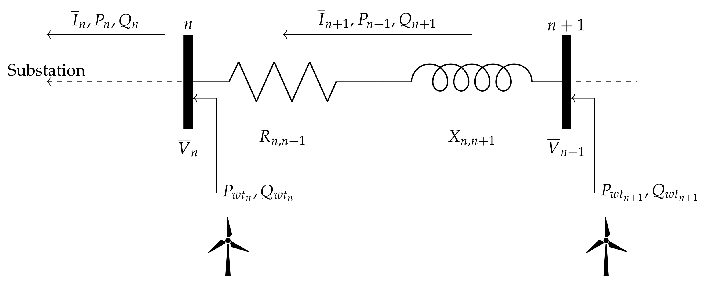
As referred to in Reference [5], in the study of wind farms collecting system, the short line model must be used. This is due to the fact that the networks that connect the various elements of a wind farm are not longer than hundreds of meters or a few kilometers, where the R/X ratio is high. Considering the short line model, several simplifications can be made in the model, and the cables’ shunt admittance can be neglected. Therefore, the network branches can be represented by the model of Figure 1, where active ($P_n$) and reactive ($Q_n$) power flows between the buses are calculated by using Equations (1) and (2), respectively. The bus voltage is calculated using Equation (3) [28]. In this model, the turbines are represented as injector points of active and reactive power in the collecting system.

$$P_n=P_{n+1}+P_{{\mathrm{wt}}_n}-R_{n,n+1}·\frac{P_{n+1}^2+Q_{n+1}^2}{|V_{n+1}{|}^2},$$

(1)

$$Q_n=Q_{n+1}+Q_{{\mathrm{wt}}_n}-X_{n,n+1}·\frac{P_{n+1}^2+Q_{n+1}^2}{|V_{n+1}{|}^2},$$

(2)

$$|V_n{|}^2={\left|V_{n+1}\right|}^2-2(R_{n,n+1}{P}_{n+1}+X_{n,n+1}{Q}_{n+1})+(R_{n,n+1}^2+X_{n,n+1}^2).\frac{P_{n+1}^2+Q_{n+1}^2}{|V_{n+1}{|}^2}.$$

(3)

where $R_{n,n+1}$ and $X_{n,n+1}$ represents the branch resistance and reactance between buses n and $n+1$, respectively. Considering

$$I_{n+1}^2=\frac{P_{n+1}^2+Q_{n+1}^2}{|V_{n+1}{|}^2},$$

(4)

the active and reactive branch losses are given by Equations (5) and (6), respectively.

$$P_{\mathrm{loss}(n,n+1)}=R_{n,n+1}·I_{n+1}^2,$$

(5)

$$Q_{\mathrm{loss}(n,n+1)}=X_{n,n+1}·I_{n+1}^2.$$

(6)

Therefore, the total power losses, $P_{\mathrm{loss}\mathrm{total}}$, can then be obtained by adding all losses from all line sections as given by

$$P_{\mathrm{loss}\mathrm{total}}=\sum _{k\in \mathcal{B}}{P}_{\mathrm{loss}(k,k+1)}+Q_{\mathrm{loss}(k,k+1)}$$

(7)

where $\mathcal{B}$ is the set of the buses in the network.

The resistance $R_{n,n+1}$ and reactance $X_{n,n+1}$ values between buses depend on the cable characteristics, namely: resistance R, inductance L, and the maximum current $I_{\mathrm{z}}$ that can support. This latter value limits the number of turbines connected through a cable. In fact, the rated current drawn by each turbine, with a rated power $P_{\mathrm{r}}$ and a U interconnection grid voltage, is defined by:

$$I_{\mathrm{r}}=\frac{P_{\mathrm{r}}}{\sqrt{3}·U·cos\phi }$$

(8)

where the value of $cos\phi$ is the turbines’ power factor. For example, assuming that $P_{\mathrm{r}}=2$ MW and $U=20$ kV, the rated current drawn by each turbine is $I_{\mathrm{r}}=57.735$ A. The $I_{\mathrm{r}}$ value restricts the cable type used in a connection depending on the number of downstream wind turbines.

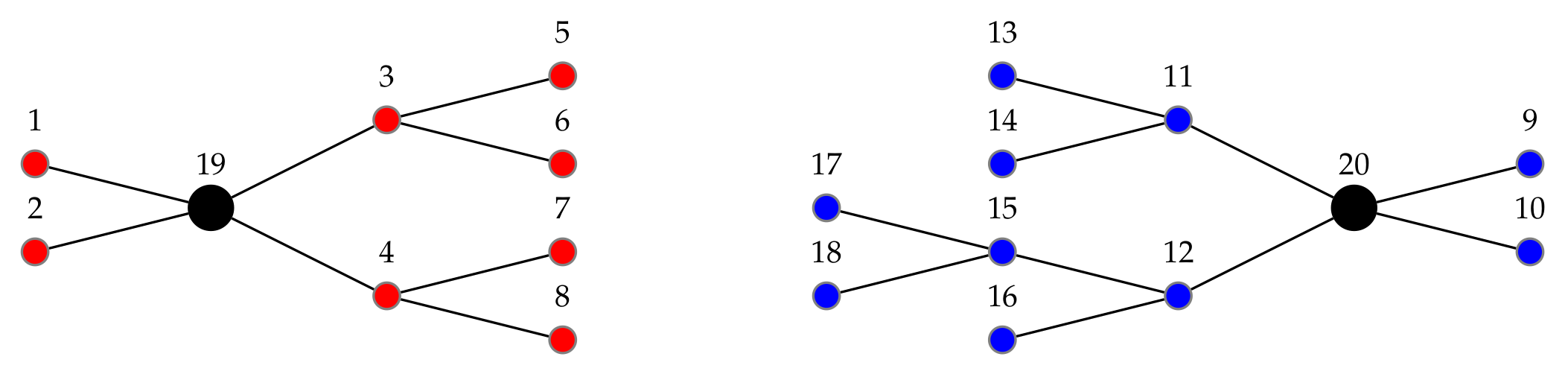
Consider the wind farm example shown in Figure 2, with two substations, nodes 19 and 20, and eighteen wind turbines, nodes 1 to 18. This layout has four branch lines connected to each substation. The total current reaching a substation from a branch line is the sum of the currents drawn by all turbines connected through this branch. For example, the branch starting in connection $(19,3)$ supports three wind turbines (including turbine 3), and so, the current crossing this cable is $3\times I_{\mathrm{r}}=173.22$ A. The branch starting in connection $(20,12)$ supports five wind turbines (including turbine 12), and so, the current crossing this cable is $5\times I_{\mathrm{r}}=288.68$ A.

In this work, the available cable types are presented in

Table 1. Unipolar cable characteristics (LXHIOV) 18/30 kV.

Type	Section	Inductance	Electrical Resistance	Max. Current	Price
k	(mm${}^2$)	L (mH/km)	R ($\mathbf{\Omega }/$km)	${\mathit{I}}_{\mathbf{z}}$ (A)	C (EUR/m)
1	050	0.62	0.6410	169	06.80
2	070	0.59	0.4430	207	07.12
3	095	0.57	0.3200	247	07.98
4	120	0.55	0.2530	281	08.70
5	150	0.54	0.2060	313	12.77
6	185	0.53	0.1640	354	13.23
7	240	0.50	0.1250	408	14.89
8	300	0.49	0.1000	458	17.50
9	400	0.47	0.0778	519	21.09
10	500	0.46	0.0605	585	23.77

. So, in the connection $(19,3)$ of Figure 2 a cable type less than $k=2$ cannot be used, which has $I_{\mathrm{z}}=207$ A, and in connection $(20,12)$ a cable type less than $k=5$ cannot be used, which has $I_{\mathrm{z}}=313$ A.

Among all the available cable types, the one with the highest $I_{\mathrm{z}}$ value is $k=10$ with $I_{{\mathrm{z}}_{10}}=585$ A. So, in the case that $I_{\mathrm{r}}=57.735$ A, any branch line cannot have more than $⌊\frac{I_{{\mathrm{z}}_{10}}}{I_{\mathrm{r}}}⌋=⌊\frac{585}{57.7}⌋=10$ wind turbines, where $\lfloor a\rfloor$ denotes the maximum integer not greater than a.

3. Mathematical Formulation

This section presents an Integer Linear Programming (ILP) model to obtain the optimal wind farm layout considering the topology and cables connection simultaneously for wind farms with several substations.

3.1. Data Sets and Parameters

Consider the node-sets $N=\{1,\cdots ,n\}$, corresponding to wind turbines location and $S=\{n+1,\cdots ,n+s\}$ corresponding to substation locations. The goal is to obtain the wind-farm connection layout, i.e., a spanning forest of a graph, $G=(V,A)$ with $V=N\cup S$ and $A=\left\{\right(i,j):i\in S,j\in N\}\cup \left\{\right(i,j):i\in N,j\in N,i\ne j\}$ where the root of each spanning trees is a node belonging to set S.

In the layout problem is considered the set of available cable types $K=\{1,\cdots ,k\}$ presented in Table 1. The maximum current intensity $I_{{\mathrm{z}}_k}$ that each cable type $k\in K$ can support bounds the number of downstream wind turbines for this cable by $⌊\frac{I_{{\mathrm{z}}_k}}{I_{\mathrm{r}}}⌋$. So, the maximum number of wind turbines in any branch line is:

$$Q=\underset{k\in K}{max}⌊\frac{I_{{\mathrm{z}}_k}}{I_{\mathrm{r}}}⌋.$$

(9)

Therefore, the number of downstream wind turbines that each connection $(i,j)$ can support, being node i in the substation side, is:

$$\mathcal{Q}\left(i\right)=\left\{\begin{array}{cc}Q\hfill & ,i\in S\hfill \\ Q-1\hfill & ,i\in N\hfill \end{array}\right..$$

(10)

Another parameter to consider is the F parameter that represents the maximum number of connections that can be linked to the substation, called feeders.

3.2. Costs

The total cost is given by the sum of the costs of active losses, $c_{\mathrm{p}}$, and reactive losses, $c_{\mathrm{q}}$, during the expected wind farm lifetime, and the infrastructure cost, $c_{\mathrm{I}}$, which includes the cable costs and digging cost.

For all pairs of nodes $(i,j)\in A$ it is known the distance ${\ell }_{ij}$, in meters, between them. By using Equations (5) and (6), the cost of the active and reactive losses, during the wind farm lifetime, in a connection $(i,j)$ supporting t downstream turbines, using a three-phase cable of type k, are, respectively,

$${c_p}_{ij}^{kt}=3·h·c_{\mathrm{e}p}\frac{{\ell }_{ji}·R_k}{{10}^3}·t^2·l_{\mathrm{f}}^2·I_{\mathrm{r}}^2,$$

(11)

and

$${c_q}_{ij}^{kt}=3·h·c_{\mathrm{e}q}\frac{{\ell }_{ji}·\omega ·L_k}{{10}^6}·t^2·l_{\mathrm{f}}^2·I_{\mathrm{r}}^2$$

(12)

where h is the number of hours during the expected wind farm lifetime, $c_{\mathrm{e}p}$ is the active energy cost, $c_{\mathrm{e}q}$ is the reactive energy cost, and $l_{\mathrm{f}}$ is the load factor which reflects the real operating conditions during the wind farm lifetime; $\omega$ is the angular frequency.

The infrastructure cost to make a cable connection $(i,j)$ using a cable of a type k is

$${c_{\mathrm{I}}}_{ij}^k=(D+3·C_k)·{\ell }_{ij},$$

where D is the digging cost (EUR by meter) and $3·C_k$ is the three-phase cable cost (EUR by meter).

Following [3], a preprocessing calculus is performed to determine the optimal cable type, $k_{ij}^t$, for a connection $(i,j)$ supporting the current of t downstream wind turbines,

$$\begin{array}{c}\hfill {\displaystyle k_{ij}^t=arg\underset{k\in K:t·I_{\mathrm{r}}\le I_{{\mathrm{z}}_k}}{min}\left({c_{\mathrm{I}}}_{ij}^k+{c_p}_{ij}^{kt}+{c_q}_{ij}^{kt}\right),}\end{array}$$

(13)

and the correspondent cost,

$$\begin{array}{c}\hfill T_{ij}^t={c_{\mathrm{I}}}_{ij}^{k_{ij}^t}+{c_p}_{ij}^{k_{ij}^{t}t}+{c_q}_{ij}^{k_{ij}^{t}t}\end{array}$$

(14)

is the minimum cost for the connection $(i,j)$ with t downstream turbines.

3.3. Decision Variables

The decision variables are:

• For all $(i,j)\in A$, binary variables $x_{ij}^t$ taking value 1 if the nodes i and j are connected (being node i on the substation side) and supports the current of t downstream wind turbines (including the one located in j); otherwise, it takes value zero.
• For all $i\in S$, binary variables $w_i$ taking value 1 if substation i is in the solution; otherwise, it takes value zero.

3.4. Cable Connection Layout Model

The ILP model to optimize the wind farm layout considering multiple substations, WFLMS, is given by:

$${\displaystyle min\sum _{(i,j)\in A}\sum _{t=1}^{\mathcal{Q}\left(i\right)}{T}_{ij}^t·x_{ij}^t}$$

(15)

$$\begin{array}{cc}& \mathrm{s}\mathrm{u}\mathrm{b}\mathrm{j}\mathrm{e}\mathrm{c}\mathrm{t} \mathrm{t}\mathrm{o}\hfill \end{array}$$

$$\begin{array}{cc}& \sum _{i\in S}\sum _{j\in N}\sum _{t=1}^Q\left(t·x_{ij}^t\right)=n\hfill \end{array}$$

(16)

$$\begin{array}{cc}& \sum _{j\in N}\sum _{t=1}^Q{x}_{ij}^t\le F·w_i,i\in S\hfill \end{array}$$

(17)

$$\begin{array}{cc}& \sum _{i\in V}\sum _{t=1}^{\mathcal{Q}\left(i\right)}{x}_{ij}^t=1,j\in N\hfill \end{array}$$

(18)

$$\begin{array}{cc}& \sum _{i\in V}\sum _{t=1}^{\mathcal{Q}\left(i\right)}\left(t·x_{ij}^t\right)-1=\sum _{i\in N}\sum _{t=1}^{\mathcal{Q}\left(i\right)}\left(t·x_{ji}^t\right),j\in N\hfill \end{array}$$

(19)

$$\begin{array}{cc}& x_{ij}^t\in \{0,1\},(i,j)\in A,t=1,\cdots ,\mathcal{Q}\left(i\right)\hfill \end{array}$$

(20)

$$\begin{array}{cc}& w_i\in \{0,1\},i\in S\hfill \end{array}$$

(21)

The objective function (15) minimizes the total cost layout. Equation (16) guarantees that the network connects n wind turbines. Constraints (17) impose the maximum number of feeders, F, that can enter each substation. Constraints (18) guarantee that each wind turbine $j\in N$ has one incoming connection. Constraints (19) are the flow conservation constraints and guarantee that for each wind turbine $j\in N$, if there exists an incoming connection supporting t downstream wind turbines, then the outgoing connections from turbine j must support $t-1$ downstream wind turbines. Finally, constraints (20) and (21) are the variable domain constraints.

3.5. Bounding Connections

If it is desired to bound the number of connections between a set of turbines, B, to the remaining wind turbines and substations, the following constraint must be included,

$$\sum _{j\in B}\sum _{i\in V,i\notin B}\sum _{t=1}^{\mathcal{Q}\left(i\right)}{x}_{ij}^t+\sum _{j\in B}\sum _{i\in N,i\notin B}\sum _{t=1}^{\mathcal{Q}\left(j\right)}{x}_{ji}^t\le L$$

(22)

where L is the maximum number of links between set turbines, B, to the remaining wind turbines and substations.

3.6. Substations Selection

The model WFLMS enables one to determine also the set of substations to include in the solution. So, it can be used to determine the best substation locations as long as a discrete set of substation locations is available. Furthermore, if a maximum number, M, of substations to be present in the solution is predefined, only Constraint (23) needs to be included.

$$\sum _{i\in S}{w}_i\le M.$$

(23)

3.7. General Comments

It is also possible to incorporate in model WFLMS the topology of the wind turbines farm, choosing a given number of turbines from a set of possible locations of wind turbines. This is done by enlarging the turbine’s set, N, to the set of possible locations of the turbines from which it is intended to choose n turbines. In terms of the optimization model, it is not necessary to change the model, it is only necessary to extend the data files.

To take into account the real landscape and forbidden zones, it is necessary to compute the distances between the nodes in order to contemplate the ground situation.

4. Results and Discussion of the Case Studies

This section presents and discusses the obtained results using the proposed model to optimize the layout of two wind farms, WF-102-S2 and WF-74-S3, generated according to examples found in [29,30]. The first one has two substations and 102 wind turbines, while the second one has 74 wind turbines and sixteen possible sites for a substation, of which a maximum of three are to be chosen.

In all cases, the ten cable types presented on Table 1 were considered. Additionally, it was considered: $h=24\times 365\times 20$ as the number of hours during the expected wind farm lifetime, assuming that it is 20 years; $c_{\mathrm{e}p}=102.52\times {10}^{-6}$ EUR/Wh as the cost of active energy; $c_{\mathrm{e}q}=51.26\times {10}^{-6}$ EUR/Wh as the cost of reactive energy; $l_{\mathrm{f}}=0.35$ as the load factor, which reflects the real operating conditions during the wind farm lifetime, and is the ratio between the generated current and the maximum current that can be generated; $\omega =100\pi$ rad/s as the angular frequency.

The optimization models were constructed using FICO Xpress Mosel (Xpress Mosel Version 4.8.0), and then they were solved with FICO Xpress Optimizer. Computations were performed on a computer Intel(R) Core(TM) i7-8550U CPU @ 1.80 GHz 1.99 GHz with 8GB RAM and 64 bits.

The results of each wind farm are analyzed in the following sections.

4.1. WF-102-S2 Wind Farm

The first case study is the WF-102-S2 wind farm with two substations and 102 wind turbines with $P_{\mathrm{r}}=2$ MW of rated power, interconnected by a $U=20$ kV grid. With these parameters, the rated current drawn by each turbine is $I_{\mathrm{r}}=57.735$ A, and the maximum number of wind turbines per branch line is $Q=10$. This value is due to the fact that the maximum current intensity that the available cables can support is $I_{\mathrm{z}}=585$, Table 1, and so $Q=⌊\frac{585}{57.7}⌋=10$, Equation (9).

The coordinates of the wind turbines and substations are in

Table A1. WF-102-S2 wind farm coordinates (WGS84).

No.	Latitude	Longitude	No.	Latitude	Longitude	No.	Latitude	Longitude
$0_1$	54.04470000	−3.50255000	34	54.08490000	−3.57471667	69	54.09626667	−3.63493333
$0_2$	54.07951667	−3.57511667	35	54.08981667	−3.58510000	70	54.10030000	−3.64470000
1	54.02993333	−3.44731667	36	54.10518333	−3.61761667	71	54.10380000	−3.65460000
2	54.03440000	−3.45588333	37	54.10988333	−3.62753333	72	54.01888333	−3.50275000
3	54.03886667	−3.46446667	38	54.11658333	−3.64171667	73	54.02335000	−3.51133333
4	54.04331667	−3.47305000	39	54.02441667	−3.47503333	74	54.02781667	−3.51991667
5	54.04778333	−3.48163333	40	54.02886667	−3.48361667	75	54.03226667	−3.52850000
6	54.05225000	−3.49021667	41	54.03333333	−3.49220000	76	54.03673333	−3.53708333
7	54.05671667	−3.49880000	42	54.03780000	−3.50078333	77	54.04118333	−3.54568333
8	54.06116667	−3.50740000	43	54.04226667	−3.50936667	78	54.04565000	−3.55426667
9	54.06563333	−3.51598333	44	54.04671667	−3.51795000	79	54.05010000	−3.56286667
10	54.07010000	−3.52456667	45	54.05118333	−3.52655000	80	54.05475000	−3.57295000
11	54.07455000	−3.53316667	46	54.05563333	−3.53513333	81	54.05955000	−3.58366667
12	54.07901667	−3.54176667	47	54.06010000	−3.54373333	82	54.06296667	−3.59505000
13	54.08361667	−3.55065000	48	54.06836667	−3.56223333	83	54.06450000	−3.60870000
14	54.08823333	−3.55953333	49	54.07218333	−3.57215000	84	54.06603333	−3.62235000
15	54.09283333	−3.56843333	50	54.07598333	−3.58206667	85	54.06756667	−3.63601667
16	54.09743333	−3.57731667	51	54.07980000	−3.59196667	86	54.09203333	−3.64363333
17	54.11125000	−3.60400000	52	54.08360000	−3.60190000	87	54.09580000	−3.65346667
18	54.11585000	−3.61290000	53	54.10071667	−3.62623333	88	54.01613333	−3.51660000
19	54.12045000	−3.62180000	54	54.11020000	−3.64816667	89	54.02058333	−3.52520000
20	54.12536667	−3.63128333	55	54.02165000	−3.48888333	90	54.02505000	−3.53376667
21	54.02716667	−3.46116667	56	54.02611667	−3.49746667	91	54.02950000	−3.54235000
22	54.03163333	−3.46975000	57	54.03058333	−3.50606667	92	54.03396667	−3.55095000
23	54.03610000	−3.47833333	58	54.03503333	−3.51465000	93	54.03841667	−3.55953333
24	54.04056667	−3.48691667	59	54.03950000	−3.52323333	94	54.04180000	−3.56891667
25	54.04503333	−3.49550000	60	54.04395000	−3.53181667	95	54.04603333	−3.57950000
26	54.04948333	−3.50408333	61	54.04841667	−3.54040000	96	54.04980000	−3.59058333
27	54.05395000	−3.51266667	62	54.05288333	−3.54900000	97	54.05308333	−3.60208333
28	54.05840000	−3.52126667	63	54.05733333	−3.55758333	98	54.05588333	−3.61396667
29	54.06286667	−3.52986667	64	54.06156667	−3.56758333	99	54.05816667	−3.62616667
30	54.06733333	−3.53845000	65	54.06580000	−3.57758333	100	54.05991667	−3.63860000
31	54.07178333	−3.54705000	66	54.06933333	−3.58836667	101	54.06475000	−3.64645000
32	54.07616667	−3.55626667	67	54.07296667	−3.60095000	102	54.08780000	−3.65233333
33	54.08053333	−3.56548333	68	54.07660000	−3.61353333

.

Two scenarios are considered for this wind farm: the wind farm original, WF-102-S2, and the wind farm WF-102-S2W, which includes a limit in the sidewalk connection.

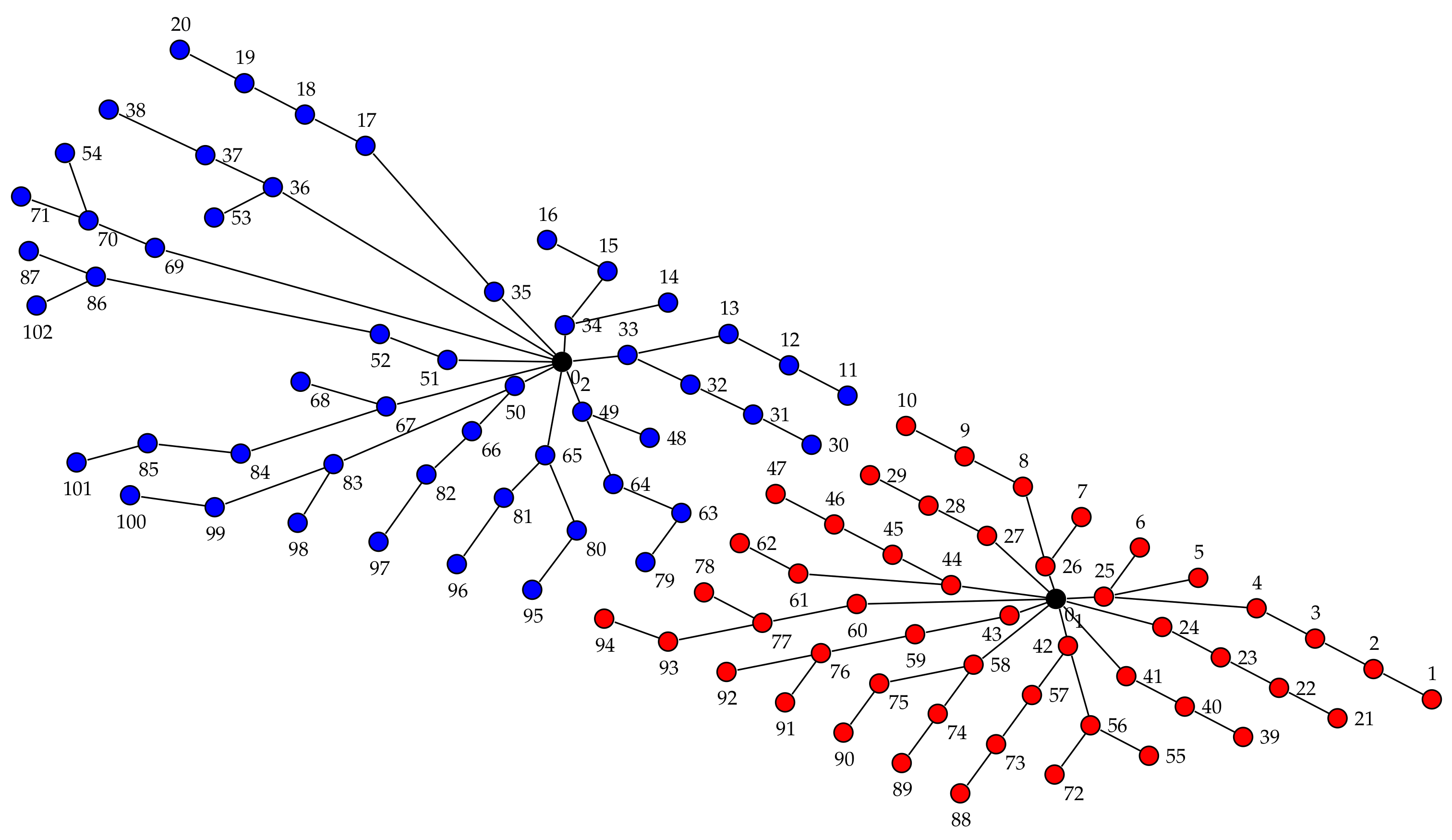
For the first scenario, WF-102-S2, the obtained cable connection layout is presented in Figure 3, the costs in the optimal solution are presented in

Table 2. Optimal costs: WF-102-S2 and WF-102-S2-W wind farm.

Case Study	Costs
	${\mathit{C}}_{\mathit{I}}$	${\mathit{C}}_{\mathit{p}}$	${\mathit{C}}_{\mathit{q}}$	Total
WF-102-S2	6,332,484.5	2,410,659.4	1,732,628.4	10,475,772.3
WF-102-S2-W	6,112,964.7	2,527,016.9	2,027,064.2	10,667,045.8

, and information about optimal cable connections is presented in

Table 3. Optimal solution cable type: WF-102-S2 and WF-102-S2-W wind farm.

Case Study	# Feeders/Substation		Connections/Cable Type
	${\mathit{O}}_1$	${\mathit{O}}_2$	3	4	7	8	10
WF-102-S2	10	10	39	22	17	10	14
WF-102-S2-W	10	10	41	23	18	6	14

.

The correspondent model WFLMS for this scenario has 207 constraints and 94,758 variables, and the processing time to obtain the optimal solution was 79 s.

The total cost obtained is EUR 10,475,772.3, where 60.5% is the infrastructure cost, corresponding to EUR 6,332,484.5, 23.0% is the active losses cost, corresponding to EUR 2,410,659.4, and 16.5% is the reactive losses cost, corresponding to EUR 1,732,628.4. The highest amount corresponds to the infrastructure cost, and the smallest part is the reactive losses cost during wind farm lifetime. Table 3 shows information about the cable types being used in the optimal solution. In the optimal solution, only five different types of cables are used: type 3 in 41 connections, type 4 in 23 connections, type 7 in 18 connections, type 8 in 6 connections, and type 10 in 14 connections.

The second scenario, WF-102-S2W, is obtained by limiting to two the connections passing on the walkway, adding constraint (22) with $L=2$ in the model WFLMS.

The optimal connection layout for WF-102-S2W is presented in Figure 4 and the costs in the optimal solution are presented in Table 2.

The correspondent model has 207 constraints and 94,758 variables, and the processing time to obtain the optimal solution was 85.3 s.

In the optimal solution, only five different types of cables are used: type 3 in 39 connections, type 4 in 22 connections, type 7 in 17 connections, type 8 in 10 connections, and type 10 in 14 connections, Table 3.

The total cost is EUR 10,667,045.8, where: 57.3% is the infrastructure cost, corresponding to EUR 6,112,964.7; 23.7% is the active losses cost, corresponding to EUR 2,527,016.9; and 19.0% is the reactive losses cost, corresponding to EUR 2,027,064.2.

There are two sectors in both optimal wind farm solutions, WF-102-S2 and WF-102-S2-w: one has an installed capacity of 100 MW, with 50 wind turbines connected to substation $0_1$ and the other one has 104 MW of installed capacity, with 52 turbines connected to substation $0_2$. There are ten branch lines linked to each substation, and the number of wind turbines in each branch line ranges between four and eight turbines. In the optimal solutions, only five different types of cables are used 3, 4, 7, 8, and 10, as shown in Table 3.

Comparing both scenarios’ optimal solutions, in Table 2 and Table 3, as expected, the total cost corresponding to the optimal solution when limiting the number of connections to a subset of turbines, study case WF-102-S2-W, is higher. This phenomenon is due to the increasing of active and reactive loss costs that are not compensated by the decreasing observed in the infrastructure cost. Note that these changes in costs result from the use of lower types of cables, which are cheaper but have higher energy losses.

4.2. WF-74-S3 Wind Farm

The second wind farm, WF-74-S3, is formed by 74 turbines with $P_{\mathrm{r}}=2$ MW of rated power, interconnected by a $U=20$ kV grid. With these parameters, the rated current drawn by each turbine is $I_{\mathrm{r}}=57.735$ A, and the maximum number of wind turbines per branch line is $Q=10$. Sixteen possible positions for substations, distributed in a grid of 4 × 4-type points over the wind farm, are considered: $O_1$, $O_2$, ..., $O_{16}$. The coordinates of the wind turbines and substations are presented in

Table A2. WF-74-S3 wind farm coordinates (Cartesian).

No.	Latitude	Longitude	No.	Latitude	Longitude	No.	Latitude	Longitude
$O_1$	0639.1	0640.6	15	1800.0	1410.0	45	3000.0	3000.0
$O_2$	0639.1	1546.7	16	1800.0	1812.0	46	3000.0	3410.0
$O_3$	0639.1	2452.8	17	1375.0	1812.0	47	3000.0	3812.0
$O_4$	0639.1	3358.9	18	1000.0	2225.0	48	3800.0	3410.0
$O_5$	1542.2	0640.6	19	0600.0	1410.0	49	3800.0	3812.0
$O_6$	1542.2	1546.7	20	0187.5	1000.0	50	3800.0	1000.0
$O_7$	1542.2	2452.8	21	0600.0	1812.0	51	3000.0	1812.0
$O_8$	1542.2	3358.9	22	0187.5	1410.0	52	3375.0	1812.0
$O_9$	2445.3	0640.6	23	0187.5	1812.0	53	3375.0	2225.0
$O_{10}$	2445.3	1546.7	24	0187.5	2225.0	54	3375.0	2600.0
$O_{11}$	2445.3	2452.8	25	1375.0	2225.0	55	3800.0	2600.0
$O_{12}$	2445.3	3358.9	26	1800.0	2225.0	56	3800.0	0187.5
$O_{13}$	3348.4	0640.6	27	1800.0	2600.0	57	3800.0	1410.0
$O_{14}$	3348.4	1546.7	28	1375.0	3000.0	58	3800.0	3000.0
$O_{15}$	3348.4	2452.8	29	1000.0	3000.0	59	3375.0	3000.0
$O_{16}$	3348.4	3358.9	30	0600.0	3000.0	60	3000.0	2225.0
01	0187.5	0187.5	31	0187.5	3000.0	61	3000.0	2600.0
02	0187.5	0600.0	32	0187.5	3410.0	62	3000.0	1410.0
03	0600.0	1000.0	33	1375.0	3410.0	63	3000.0	1000.0
04	0600.0	0187.5	34	1000.0	3410.0	64	3000.0	0600.0
05	1000.0	0187.5	35	1375.0	3812.0	65	3800.0	0600.0
06	1000.0	0600.0	36	1000.0	3812.0	66	3375.0	0187.5
07	1375.0	1000.0	37	0600.0	3812.0	67	2600.0	2225.0
08	1375.0	0600.0	38	1800.0	3410.0	68	2187.5	2225.0
09	1800.0	0600.0	39	1800.0	3812.0	69	2187.5	1812.0
10	1800.0	0187.5	40	2187.5	3812.0	70	2600.0	1410.0
11	2600.0	0187.5	41	2187.5	3410.0	71	2187.5	1410.0
12	2187.5	0600.0	42	2187.5	3000.0	72	2600.0	1000.0
13	2187.5	1000.0	43	2187.5	2600.0	73	3375.0	1000.0
14	1800.0	1000.0	44	2600.0	3000.0	74	2600.0	1812.0

.

The goal is to optimize the cable layout, choosing at most three of the available substations. To solve this problem, the model WFLMS including constraint (23) with $M=3$ is considered.

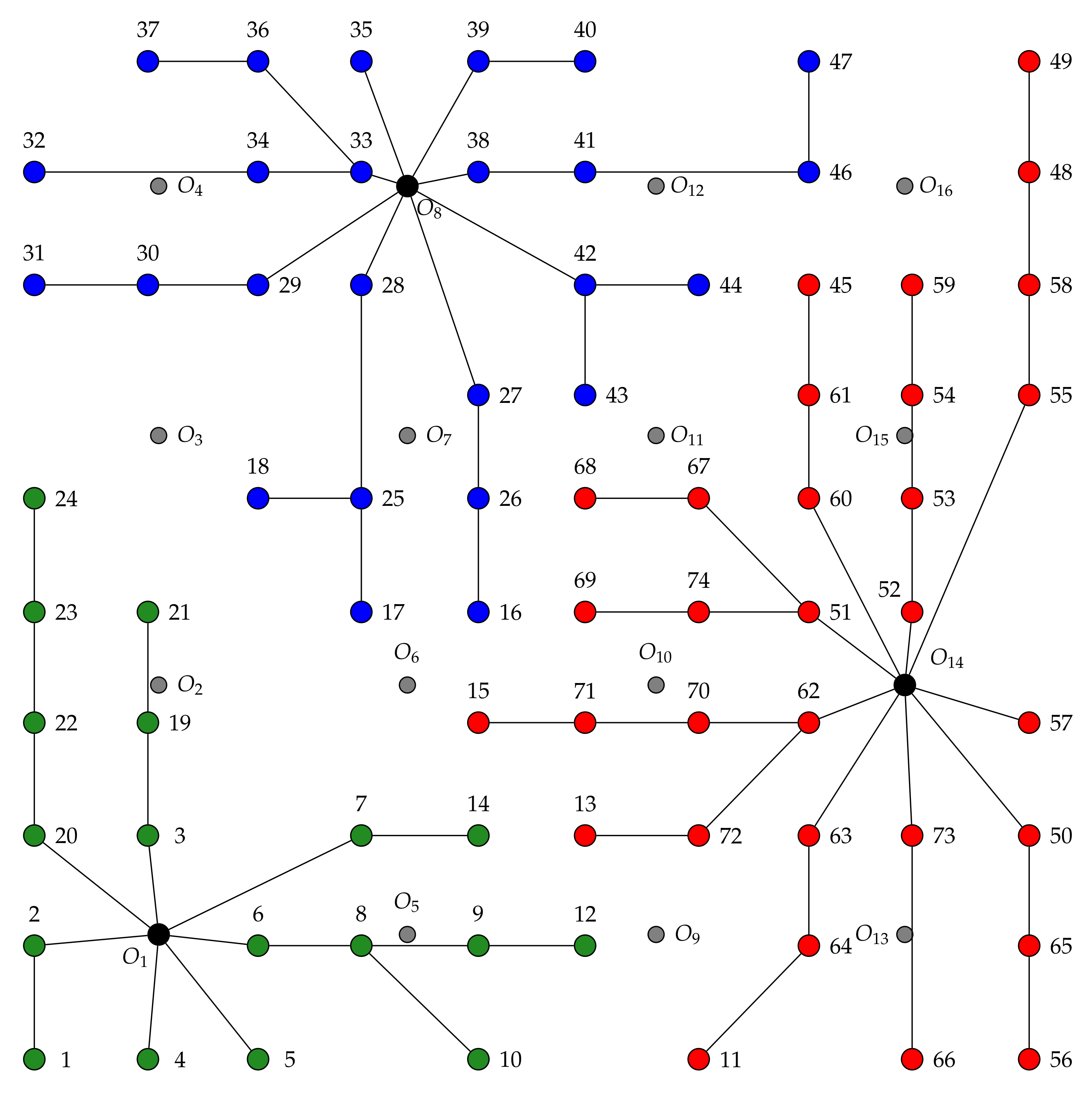
The optimal connection layout is presented in Figure 5, the costs in the optimal solution are shown in

Table 4. Optimal costs: WF-74-S3.

Case Study	Costs
	${\mathit{C}}_{\mathit{I}}$	${\mathit{C}}_{\mathit{p}}$	${\mathit{C}}_{\mathit{q}}$	Total
WF-74-S3	1,887,148.4	660,641.2	360,997.9	2,908,787.5

, and information about optimal cable connections is presented in

Table 5. Optimal solution cable type: WF-74-S3 wind farm.

Case Study	# Feeders/Substation			# Connections/Cable Type (k)
	${\mathit{O}}_{\mathbf{1}}$	${\mathit{O}}_{\mathbf{8}}$	${\mathit{O}}_{\mathbf{14}}$	3	4	7	8	10
WF-74-S3	7	8	9	30	21	13	6	4

.

The model has 166 constraints and 60,474 variables, and the processing time to obtain the optimal solution was 158.4 s.

The optimal wind farm has three sectors: one has an installed capacity of 26 MW, with 18 wind turbines connected to the substation $O_1$; the other one has 50 MW of installed capacity, with 25 turbines connected to the substation $O_8$; and the last one has 31 wind turbines connected to the substation $O_{14}$, having 62 MW.

There are seven branches connected to substation $O_1$, in which the number of turbines varies from one to five. Substation $O_8$ is linked to eight branch lines; it also has a number of turbines ranging between one and five. There are nine branch lines linked to the substation $O_{14}$, in which the number of turbines varies between one and six. In the optimal solutions, only five different types of cables are used: type 3 in 30 connections, type 4 in 21 connections, type 7 in 13 connections, type 8 in 6 connections, and type 10 in 4 connections, as shown in Table 5.

The total cost is EUR 2,908,787.57, where 64.9% is the infrastructure cost, corresponding to EUR 1,887,148.4, 22.7% is the active losses cost, corresponding to EUR 660,641.2, and 12.4% is the reactive losses cost, corresponding to EUR 360,997.9, Table 4.

Once again, the highest amount corresponds to the infrastructure cost and the lowest amount is the reactive losses cost during wind farm lifetime.

Comparing this approach with approaches in the literature, Reference [22], the presented model is much faster at finding the optimal solution.

5. Conclusions

This work presents an ILP model to solve a cable connection layout considering wind farms with several substations. The model was applied to two wind farms with up to 102 turbines. In the wind farm with 102 turbines, there are two substations, and two variants of this case study are considered: one in which the original model WFLMS is considered and another in which a new model is considered where, to meet the solution installed on the ground, the number of connections between a set of turbines and the rest of the wind farm is limited. An additional constraint was considered in the latter case study. The proposed model was able to determine the optimal solution in both variants in a very short time, around 80 s.

In a wind farm with 74 turbines, sixteen possible locations for substations are considered, and the goal is to optimize the layout of the wind farm with at most three substations. To contemplate this new issue, it is only necessary to include a new constraint (23), to the initially proposed model, WFLMS. The optimal solution for this case study was obtained in only 158.4 s.

To contemplate this new issue, a new constraint (23), to the initially proposed model, WFLMS, was included. The optimal solution for this case study was obtained in only 158.4 s.

The results are promising. The optimal solutions are obtained in a short time and, if desired, the number of possible locations for the substations can be increased, bringing the discretized problem closer to the problem of choosing the best locations globally across the park.

The proposed model can also consider forbidden zones and can be adapted to optimize also the topology of the wind turbines farm, choosing a given number of turbines from a set of possible locations of wind turbines. Furthermore, compared with the literature, the presented model is fast at finding the optimal solution.

References

- Directive (EU) 2018/2001 on the promotion of the use of energy from renewable sources. Off. J. Eur. Union 2018, L 328, 209.
- Cerveira, A.; Baptista, J.; Solteiro Pires, E.J. Optimization Design in Wind Farm Distribution Network. In International Joint Conference SOCO’13-CISIS’13-ICEUTE’13; Herrero, Á., Baruque, B., Klett, F., Abraham, A., Snášel, V., de Carvalho, A.C., Bringas, P.G., Zelinka, I., Quintián, H., Corchado, E., Eds.; Springer International Publishing: Cham, Switzerland, 2014; pp. 109–119. [Google Scholar]
- Cerveira, A.; de Sousa, A.; Solteiro Pires, E.J.; Baptista, J. Optimal Cable Design of Wind Farms: The Infrastructure and Losses Cost Minimization Case. IEEE Trans. Power Syst. 2016, 31, 4319–4329. [Google Scholar] [CrossRef]
- Wędzik, A.; Siewierski, T.; Szypowski, M. A new method for simultaneous optimizing of wind farm’s network layout and cable cross-sections by MILP optimization. Appl. Energy 2016, 182, 525–538. [Google Scholar] [CrossRef]
- Cerveira, A.; Baptista, J.; Solteiro Pires, E.J. Wind farm distribution network optimization. Integr. Comput. Aided Eng. 2016, 23, 69–79. [Google Scholar] [CrossRef]
- Fischetti, M.; Pisinger, D. Mixed Integer Linear Programming for new trends in wind farm cable routing. Electron. Notes Discret. Math. 2018, 64, 115–124. [Google Scholar] [CrossRef] [Green Version]
- Bentz, C.; Costa, M.C.; Hertz, A.; Poirion, P.L. Cabling optimization of a windfarm and capacitated K-Steiner tree. In Proceedings of the PGMO-COPI’14 Gaspard Monge Program for Optimization—Conference on Optimization Practices in Industry, Palaiseau, France, 28–30 October 2014; p. 4. [Google Scholar]
- Hertz, A.; Marcotte, O.; Mdimagh, A.; Carreau, M.; Welt, F. Optimizing the Design of a Wind Farm Collection Network. INFOR Inf. Syst. Oper. Res. 2012, 50, 95–104. [Google Scholar] [CrossRef]
- Baptista, J.; Solteiro Pires, E.J.; Cerveira, A. Wind Farm Distribution Network Optimization Based in a Hierarchical GA. In Proceedings of the ISAP2013—Seventeenth International Conference on Intelligent System Applications to Power Systems, Tokyo, Japan, 1–4 July 2013; p. 6. [Google Scholar]
- Veeramachaneni, K.; Wagner, M.; O’Reilly, U.M.; Neumann, F. Optimizing energy output and layout costs for large wind farms using particle swarm optimization. In Proceedings of the 2012 IEEE Congress on Evolutionary Computation, Brisbane, Australia, 10–15 June 2012; pp. 1–7. [Google Scholar] [CrossRef]
- Qi, Y.; Hou, P.; Yang, L.; Yang, G. Simultaneous Optimisation of Cable Connection Schemes and Capacity for Offshore Wind Farms via a Modified Bat Algorithm. Appl. Sci. 2019, 9, 265. [Google Scholar] [CrossRef] [Green Version]
- Wang, L.; Wu, J.; Han, R.; Wang, T. Minimizing Energy Loss by Coupling Optimization of Connection Topology and Cable Cross-Section in Offshore Wind Farm. Appl. Sci. 2019, 9, 3722. [Google Scholar] [CrossRef] [Green Version]
- Khanali, M.; Ahmadzadegan, S.; Omid, M.; Nasab, F. Optimizing layout of wind farm turbines using genetic algorithms in Tehran province, Iran. Int. J. Energy Environ. Eng. 2018, in press. [Google Scholar] [CrossRef] [Green Version]
- Srikakulapu, R.; U, V. Optimized design of collector topology for offshore wind farm based on ant colony optimization with multiple travelling salesman problem. J. Mod. Power Syst. Clean Energy 2018, 6, 1181–1192. [Google Scholar] [CrossRef] [Green Version]
- Wang, L.; Wu, J.; Wang, T.; Han, R. An optimization method based on random fork tree coding for the electrical networks of offshore wind farms. Renew. Energy 2020, 147, 1340–1351. [Google Scholar] [CrossRef]
- Pillai, A.; Chick, J.; Johanning, L.; Khorasanchi, M.; de Laleu, V. Offshore wind farm electrical cable layout optimization. Eng. Optim. 2015, 47, 1689–1708. [Google Scholar] [CrossRef] [Green Version]
- Lingling, H.; Yang, F.; Xiaoming, G. Optimization of electrical connection scheme for large offshore wind farm with genetic algorithm. In Proceedings of the 2009 International Conference on Sustainable Power Generation and Supply, Nanjing, China, 6–7 April 2009; pp. 1–4. [Google Scholar] [CrossRef]
- Zuo, T.; Zhang, Y.; Meng, K.; Tong, Z.; Dong, Z.Y.; Fu, Y. Collector System Topology Design for Offshore Wind Farm’s Repowering and Expansion. IEEE Trans. Sustain. Energy 2021, 12, 847–859. [Google Scholar] [CrossRef]
- Dutta, S.; Overbye, T.J. A clustering based wind farm collector system cable layout design. In Proceedings of the 2011 IEEE Power and Energy Conference at Illinois, Urbana, IL, USA, 25–26 February 2011; pp. 1–6. [Google Scholar] [CrossRef]
- Dutta, S.; Overbye, T. Optimal Wind Farm Collector System Topology Design Considering Total Trenching Length. IEEE Trans. Sustain. Energy 2012, 3, 339–348. [Google Scholar] [CrossRef]
- Wu, Y.; Wang, Y. Collection line optimisation in wind farms using improved ant colony optimisation. Wind Eng. 2021, 45, 589–600. [Google Scholar] [CrossRef]
- Pérez-Rúa, J.A.; Stolpe, M.; Cutululis, N.A. Integrated Global Optimization Model for Electrical Cables in Offshore Wind Farms. IEEE Trans. Sustain. Energy 2020, 11, 1965–1974. [Google Scholar] [CrossRef]
- Wang, L.; Wu, J.; Tang, Z.; Wang, T. An Integration Optimization Method for Power Collection Systems of Offshore Wind Farms. Energies 2019, 12, 3965. [Google Scholar] [CrossRef] [Green Version]
- Chen, T.; Chen, M.; Hwang, K.; Kotas, P.; Chebli, E.A. Distribution system power flow analysis—A rigid approach. IEEE Trans. Power Deliv. 1991, 6, 1146–1152. [Google Scholar] [CrossRef]
- Moon, Y.H.; Choi, B.K.; Cho, B.H.; Kim, S.H.; Ha, B.N.; Lee, J.H. Fast and reliable distribution system load flow algorithm based on the Y/sub BUS/ formulation. In Proceedings of the 1999 IEEE Power Engineering Society Summer Meeting, Conference Proceedings (Cat. No.99CH36364), Edmonton, AB, Canada, 18–22 July 1999; Volume 1, pp. 238–242. [Google Scholar] [CrossRef]
- Gómez Expósito, A.; Romero Ramos, E. Reliable load flow technique for radial distribution networks. IEEE Trans. Power Syst. 1999, 14, 1063–1069. [Google Scholar] [CrossRef]
- Baran, M.E.; Wu, F.F. Optimal capacitor placement on radial distribution systems. IEEE Trans. Power Deliv. 1989, 4, 725–734. [Google Scholar] [CrossRef]
- Haque, M. Efficient load flow method for distribution systems with radial or mesh configuration. IEE Proc. Gener. Transm. Distrib. 1996, 143, 33–38. [Google Scholar] [CrossRef]
- Seafish. Kingfisher Wind Farms Chart: Walney 1–3 Offshore Wind Farm. 2021. Available online: https://kis-orca.org/downloads/ (accessed on March 2021).
- Pricope, R.; Neagu, B. Optimal Reconfiguration of a Wind Farm Power Distribution Network. Bul. Inst. Politeh. Din Iasi 2015, LXI, 91–101. [Google Scholar]
Figure 1.
Line diagram of a radial distribution system.
Figure 2.
Wind farm layout example.
Figure 3.
Optimal cable connection layout for WF-102-S2 wind farm.
Figure 4.
Optimal cable connection layout for WF-102-S2-W wind farm.
Figure 5.
Optimal cable connection layout for the WF-74-S3 wind farm.