Modeling Electricity Price and Quantity Uncertainty: An Application for Hedging with Forward Contracts

Abstract

Energy transactions in liberalized markets are subject to price and quantity uncertainty. This paper considers the spot price and energy generation to follow a bivariate semi-nonparametric distribution defined in terms of the Gram–Charlier expansion. This distribution allows us to jointly model not only mean, variance, and correlation but also skewness, kurtosis, and higher-order moments. Based on this model, we propose a static hedging strategy for electricity generators that participate in a competitive market where hedging is carried out through forward contracts that include a risk premium in their valuation. For this purpose, we use Monte Carlo simulation and consider information from the Colombian electricity market as the case study. The results show that the volume of energy to be sold under long-term contracts depends on each electricity generator and the risk assessment made by the market in the forward risk premium. The conditions of skewness, kurtosis, and correlation, as well as the type of the employed risk indicator, affect the hedging strategy that each electricity generator should implement. A positive correlation between the spot price and energy production tends to increase the hedge ratio; meanwhile, negative correlation tends to reduce it. The increase of forward risk premium, on the other hand, reduces the hedge ratio.

1. Introduction

Electricity is usually traded in a short-term market (spot market) and a long-term market via contracts for future delivery (forward contracts). The electricity market is characterized by being highly volatile when compared to other commodity markets. This high volatility in terms of price and quantity is due to market circumstances (e.g., expectations or strategies of each company and economic dynamics) and physical conditions (e.g., climate, water availability, fuel production, or damage to the power transmission network [1]).

Electricity trading implies the consideration of three main characteristics: (i) the limitation of storage for large amounts of electricity and long periods, (ii) the technical difficulties or environmental and social restrictions for long-distance transmission, and (iii) the intensive use of capital required for expanding systems at a large scale, which presents long and uncertain payback periods. Under those conditions, multiple uncertainties exist in both the electric power system and market operation. As far as the electric power system is concerned, the need for preserving the stability of the system involves different issues—e.g., economic dispatch, unit commitment, optimal power flow and power system expansion planning—that are subject to various uncertainties, including demand variations, transmission interruptions, generator failure, fuel availability, weather conditions, as explained by [2,3], and regulatory modifications, among other causes. Those real-time conditions affect the electricity pricing and imply uncertainties over the financial results for the market agents (sellers and buyers) that can drive to significant financial losses or even bankruptcy [4]. These uncertainty levels are rising due to the increase of renewable energy sources in electric power systems [5]. All of these factors explain how reliable and economically viable operations of electric power systems depend on a collection of optimization problems to coordinate electric power systems.

To achieve the best results for electricity generators, reduce their risk levels, and reach their business objectives, they must define the quantity of electricity to be sold through forward contracts and to be traded at a spot price. It should be noted that electricity generators face price and quantity uncertainty, unlike in other types of financial products; Ref. [6] explains the spot price volatility, because electricity cannot be economically stored and must be produced instantaneously to satisfy the demand. In these circumstances, ref. [7] considers the implications of load uncertainty that cannot be perfectly hedged applying financial derivatives. Ref. [8] describes how demand unpredictability is a regular matter for any commodity. Holding inventory is an answer to mitigate quantity risk for those commodities that can be economically stored; this is mentioned by [9] as a limitation to execute intertemporal arbitrage in electricity markets.

Quantity risk (or volumetric risk) is driven by different conditions, such as the economic cycle, fuel availability, hydrologic inflows, or climate. These conditions also affect price; hence, generated quantity and price tend to be correlated. Due to the limitations regarding electricity storage for extended periods (i.e., months or years), the cost-of-carry valuation is not applicable to value the theoretical forward price. Therefore, market agents set the forward price based on their expectations and the risks they assume, which gives rise to the forward risk premium (FRP).

This FRP has been studied by [10,11] for the Pennsylvania–New Jersey–Maryland (PJM) electricity market; Ref. [12] for the Nord Pool; Ref. [13] for the Colombian electricity market; Ref. [14] for the European Electricity Exchange (EEX); and [15] for the British electricity market [16]. The incorporation of an FRP immediately leads to a difference between the forward price and the spot price expectations. Regarding the behavior of uncertainty sources, the literature studies typically address the hedging problem in electricity markets by assuming normality either on the variables or on their logarithm. Although this is a common assumption—used by [7,8], and [17], among other authors—to properly select the number of forward contracts to hedge the risk associated with transactions in electricity markets, it presents limitations to deal with problems that involve cases of skewness and kurtosis.

Nevertheless, ref. [18] indicates that some variables in electricity markets exhibit conditions of skewness and kurtosis and higher-order moments that are not adequately represented only using normal distributions. These authors show that semi-nonparametric (SNP) distributions allow a better fit for hydrologic inflows, spot price, and even demand for electricity data. Ref. [19] shows that SNP distributions serve to treat historical variables featuring skewness and heavy tails. Ref. [20] uses SNP modeling to describe the co-movements of price and volume in the stock market of the United States (US), and [21] also employs the SNP distribution to model returns in the US and United Kingdom (UK) stock markets. Other works that adopt SNP approaches to expand series beyond the traditional normal or lognormal distributions are those by [22], who measures the productivity of researchers worldwide, and [23], who estimates the size distribution of US firms.

In this study, we go a step further by considering the uncertain components of each electricity generator’s price and energy generation understudy to follow a joint SNP distribution. Ref. [24] described this type of distribution and explained how it is estimated, and more recently, refs. [25,26] applied related densities to forecast financial variables. However, to the best of our knowledge, this is the first attempt to model electricity markets in a multivariate SNP framework. Furthermore, the joint modeling of price and quantity through a SNP distribution allows us to capture not only the correlation between both variables but also the dependence between all moment structures. All of these features pay a fundamental role on the risk positions of electricity generators and their strategies.

As a direct application of the model, we propose a static hedging strategy for electricity generators that participate in a competitive market where hedging is carried out through forward contracts that include a risk premium in their valuation. We consider the spot price and energy generation variables to follow a bivariate SNP distribution in terms of the Gram–Charlier expansion. This distribution allows us to not only model the mean, the variance, and their correlation but also the skewness, the kurtosis, and higher-order moments. We employ Monte Carlo simulation to analyze the effect of three risk indicators (standard deviation, value-at-risk (VaR), and conditional VaR (CVaR) on energy sales. We consider the Colombian electricity market as the case study, where the energy sources are predominant renewables.

The main contribution of the paper to the analysis of electricity markets is the structuring of an energy portfolio that does not impose the assumption of normality in both price and energy generation. The results show that the optimal quantity of energy to be sold through forward contracts is dependent not only on the conditions of spot price and quantity uncertainty but also on the way market agents weigh the assumed risk levels. Particularly, this methodology is used for hydropower generators affected by flow regimen aspects. Furthermore, the number of forward sales is determined by the correlation between price and energy generation and the FRP.

The rest of the paper is structured as follows. Section 2 introduces the mathematical model and the methodology implemented to jointly model prices and quantity uncertainty. Section 3 describes the data used in the case study. Section 4 discusses the results, analyzing the sensitivity of the risk of forward energy contracts not only to the SNP density characteristics but also to the rest of the elements of the forward contracts. Finally, Section 5 draws the main conclusions.

2. Model and Methodology

Electricity generators tend to hedge their sales of energy, which they may supply through self-generation or spot purchases. Ref. [7] proposes the hedging strategy of electricity generator i as an optimization problem with a mean–variance utility function over its net energy sales $\left(I^i\right)$. This problem is represented by Equation (1) and depends on the level of risk aversion ${\lambda }^i$. The mean–variance utility function exhibits limitations when the forward price does not match the expected spot price, i.e., when there is an FRP. Ref. [17] states that when there is a risk premium in electricity markets, the optimization of the mean–variance utility function is subject to the decision makers’ level of risk aversion, as illustrated in Equation (1), where $E\left[I^i\right]$ represents the expected utility of generator i on the decision variable $I^i$.

$$\begin{array}{cc}max& E\left[I^i\right]-{\lambda }^i\cdot E[{\left( I^i-E\left[I^i\right]\right)}^2]\end{array}$$

(1)

We consider an electricity generator i that faces uncertainty over its net sales at time $T$; therefore, it decides to sell long-term electricity contracts beforehand starting from time ($t=t_0$). If such a generator participated in an electricity market whose spot price and energy generation derived from a multivariate SNP distribution, our research question is: how many contracts should it trade to hedge its risk?

2.1. Spot Price and Energy Generation

We propose modeling these two variables through multivariate SNP functions. Below, we describe the portfolio multivariate SNP distribution, which generalizes the multivariate normal in terms of Gram–Charlier (Type A) series for every portfolio variable. Let us assume that $Z_t$ is a vector that contains J variables distributed with zero mean and multivariate SNP distribution. Its joint probability density function (pdf) $F_Z$ is written, as proposed by [24], as follows:

$$F_Z\left(Z_t\right)=G_Z\left(Z_t\right)+\left[{{\displaystyle \prod }}_{j=1}^J\frac{1}{{\sigma }_j}{g}_{z_j}\left(\frac{z_{jt}}{{\sigma }_j}\right)\right]\left[{{\displaystyle \sum }}_{j=1}^J{k}_{z_j}\left(\frac{z_{jt}}{{\sigma }_j}\right)\right] ;-\infty <z_{jt}<\infty$$

(2)

where $G_Z\left(Z_t\right)$ is a multivariate normal pdf with zero mean, covariance matrix $\Sigma$—with general element $\left\{{\sigma }_{ij}\right\}$ and marginal pdfs represented by $\frac{1}{{\sigma }_j}{g}_{z_j}\left(\frac{z_{jt}}{{\sigma }_j}\right)$—i.e., $z_{jt}~N(0,{\sigma }_j^2)$ and $v_{jt}=z_{jt}/{\sigma }_j~N\left(0,1\right)$, ${\sigma }_j^2={\sigma }_{jj}$; and $k_{z_j}\left(v_{jt}\right)$ is a linear combination of the first $M_j$ terms of the Gram–Charlier series Hermite polynomial, as shown in Equation (3). The terms of these expansions, $H_m\left(v_{jt}\right),$ is the so-called Hermite polynomials (HP) or order m—see Equation (5), which is weighted by parameter $d_{jm}$ capturing the raw moment of order m for the marginal variable j.

$$k_{z_j}\left(z_{jt}\right)={{\displaystyle \sum }}_{m=2}^{M_j}{d}_{jm}{H}_m\left(\frac{z_{jt}}{{\sigma }_j}\right)$$

(3)

Hence, the marginal pdf of $z_{jt}$ is:

$$f_{z_j}\left(z_{jt}\right)=\frac{1}{{\sigma }_j\sqrt{2\pi }}exp\left\{-\frac{1}{2}{\left(\frac{z_{jt}}{{\sigma }_j}\right)}^2\right\}\left\{1+{{\displaystyle \sum }}_{m=2}^{M_j}{d}_{jm}{H}_m\left(\frac{z_{jt}}{{\sigma }_j}\right)\right\}$$

(4)

Note that the univariate Gram–Charlier density in Equation (4) is an expansion of a normal pdf in terms of orthogonal polynomials—as described in Equation (7) below—and truncated at an arbitrary order $M_j$ that depends on the degree of accuracy and flexibility required for the SNP approximation. It can be easily proven that the even (odd) moment of order r of variable $z_{jt}$ depends linearly on $d_{jm}$ for all j ≤ r and j even (odd). Particularly, mean and variance are $E\left[z_{jt}\right]=0$ and $E\left[z_{jt}^2\right]=\left(1+2d_{j2}\right){\sigma }_j^2$, respectively, and the covariance between the variables $z_{jt}$ and $z_{it}$ is defined by the corresponding entry in matrix $\Sigma$, i.e., $E\left[z_{jt}{z}_{it}\right]={\sigma }_{ji}$. Furthermore, if $d_{j3}>0$ ($d_{j3}<0$), then the j-th marginal pdf features positive (negative) skewness, when $d_{j4}>0$ the marginal pdf of $z_{jt}$ exhibits leptokurtosis, and the higher-order even parameters account for extreme values. A further discussion on the interpretation of such parameters can be found in the studies by [18,21,23] for the case of electricity markets.

The main advantage of the SNP modeling lies in its ability to capture the full density (skewness, kurtosis, higher order moments, and their dependencies) with a flexible formulation. As a matter of fact, the asymptotic Gram–Charlier expansion captures the true underlying distribution. However, the truncated expansions might present positivity problems that are traditionally tackled through positive transformations—see, e.g., refs. [20,27], analyzing positivity surfaces [28] or implementing controlled optimization [21]. In this paper we opt for the latter method since constrained/transformed SNP densities may also present convergence problems due to complex nonlinearities among the moment structure—see, e.g., ref. [29].

The HP of order m, $H_m\left(v_{jt}\right)$ is defined in terms of the m-th derivative of the standard normal pdf, $g\left(v_{jt}\right)=\frac{1}{2\pi }{e}^{-\frac{v_{jt}{}^2}{2}}$, and thus, can be calculated by solving Equation (5).

$$H_m\left(v_{jt}\right)=\frac{{\left(-1\right)}^m}{g\left(v_{jt}\right)}\cdot \frac{d^{m}g\left(v_{jt}\right)}{d{v}_{jt}{}^m}$$

(5)

Hence, the first five HPs used to represent the standardized random variable $v$ are:

$$\begin{gathered} H_0\left(v_{jt}\right)=1 \\ {H}_1\left(v_{jt}\right)=v_{jt} \\ {H}_2\left(v_{jt}\right)=v_{jt}{}^2-1 \\ {H}_3\left(v_{jt}\right)=v_{jt}{}^3-3v_{jt} \\ {H}_4\left(v_{jt}\right)=v_{jt}{}^4-6v_{jt}{}^2+3 \\ {H}_5\left(v_{jt}\right)=v_{jt}{}^5-10v_{jt}{}^3+15v_{jt} \end{gathered}$$

(6)

It is noteworthy that the HPs form an orthonormal basis, since:

$$\int H_s\left(v_{jt}\right)H_m\left(v_{jt}\right)g\left(v_{jt}\right)d{v}_{jt}=0 Ɐs\ne m.$$

(7)

Next, we define the joint SNP pdf for spot price and energy generation. Let $p_T$ be the natural logarithm of the spot price $P_T$ and $q_T^i$, that of the energy generation by generator i. We assume that $p_T$ and $q_T^i$ are governed by a bivariate SNP process on the stochastic standardized (i.e., zero mean and unit variance) variables ${ϵ}_t^p$ and ${ϵ}_t^{q^i}$ with correlation coefficient ${\rho }_{p{\mathrm{q}}^{\mathrm{i}}}$, whose joint pdf is given by:

$$F_{ϵ}\left({ϵ}_t^p,{ϵ}_t^{q^i}\right)=G_{ϵ}\left({ϵ}_t^p,{ϵ}_t^{q^i}\right)+g\left({ϵ}_t^p\right)\cdot g\left({ϵ}_t^{q^i}\right)\cdot \left\{k_p\left({ϵ}_t^p\right)+k_{q^i}\left({ϵ}_t^{q^i}\right)\right\}$$

(8)

$G_{ϵ}\left({ϵ}_t^p,{ϵ}_t^{q^i}\right)$ being a standardized bivariate normal pdf with correlation ${\rho }_{p{\mathrm{q}}^{\mathrm{i}}}$ and $g\left({ϵ}_t^p\right)$ and $g\left({ϵ}_t^{q^i}\right)$ N (0, 1) pdf.

Thus, marginal distributions can be written as follows (see proof in Appendix A):

$$\begin{gathered} f_P\left({ϵ}_t^p\right)=g\left({ϵ}_t^p\right)+g\left({ϵ}_t^p\right)\cdot \left\{k_p\left({ϵ}_t^p\right)\right\} \\ {f}_{q^i}\left(q_T^i\right)=g\left({ϵ}_t^{q^i}\right)+g\left({ϵ}_t^{q^i}\right)\cdot \left\{k_{q^i}\left({ϵ}_t^{q^i}\right)\right\} \end{gathered}$$

(9)

where $k_p\left({ϵ}_t^p\right)={\displaystyle \sum }_{m=2}^{M_p}{d}_{pm}{H}_m\left({ϵ}_t^p\right)$ and $k_{q^i}\left(q_T^i\right)={\displaystyle \sum }_{m=2}^{M_{q^i}}{d}_{q^{i}m}^i{H}_m\left(q_T^i\right) .$

2.2. Forward Price

If an agent purchased a forward contract at time $t_o$ to receive an amount of electricity at maturity time $T$ at price $F_T^{t_o},$ it would receive such agreed amount at maturity at the agreed price $F_T^{t_o}$. Since such electricity received at time $T$ is valued at the spot price $P_T$, its net income will be given by the difference between the spot price and the agreed price stated in the contract, as in Equation (10).

$$Long Forward Payout=P_T-F_T^{t_o}$$

(10)

The seller will be paid at the agreed price in exchange for delivering the agreed amount of electricity, which will be valued at the spot price at maturity, as the short forward payout in Equation (11). This relation is used to measure the sensitivity of the risk indicators.

$$Short Forward Payout=F_T^{t_o}-P_T$$

(11)

Some authors [30] argued that traditional cost-based valuation models are not applicable in electricity markets. The assessment of assumed risk levels is reflected in the traded contracts’ price, as demonstrated for those who studied the FRP in electricity markets. Thus, the price of an electricity forward contract agreed at time $t_0$ and a maturity T will be different from the expected spot price. This difference is known as the forward risk premium (FRP), represented by Equation (12).

$$FR{P}_T^{t_0}=E_{t_0}\left(P_T\right)-F_T^{t_o}$$

(12)

The FRP sign indicates who is the agent hedging the risk and paying for it: when the sign of the FRP is positive, the seller is the one paying for the hedging, while when it is negative, the buyer is the one paying for it. According to [13], a positive FRP value denotes a normal backwardation condition. This FRP may describe the expected spot price or the forward price based on the following relationships:

$$\begin{gathered} E_{t_0}\left(P_T\right)=F_T^{t_o}+FR{P}_T^{t_0} \\ {F}_T^{t_o}=E_{t_0}\left(P_T\right)-FR{P}_T^{t_0} \end{gathered}$$

(13)

Due to the nature of forward contracts, convergence must occur at maturity, i.e., a forward price agreed on that matures at T should be equal to the spot price, as stated by [31]. Therefore as maturity approaches, the FRP becomes null in electricity markets [17], as follows:

$$\begin{gathered} \underset{t_0\to T}{\lim }FR{P}_T^{t_0}=0 \\ \Rightarrow F_T^T=P_T \end{gathered}$$

(14)

2.3. Pay-Off Function

Assuming that an electricity generator that has produced an amount of electricity $Q_T^i$ at time $T$ sells all this electricity at the market spot price $P_T$, then its net sales $I_{T }^i$ are given by the product of the spot price and its energy generation:

$$I_T^i=P_T\cdot Q_T^i$$

(15)

At time $t=t_0$, the spot price and the energy generation values are unknown, which means that the generator is taking a risk due to variations in price and quantity. To hedge the assumed risk, the generator decides to implement certain strategy $j$ at time $t_0$, whose pay-off function is ${\varphi }_T^{ij}(Q_T^i,P_T|{\theta }_{t_0}^{ij})$; its net energy sales will be given by:

$$I_T^i=P_T\cdot Q_T^i+{\varphi }_T^{ij}(Q_T^i,P_T|{\theta }_{t_0}^{ij})$$

(16)

where ${\theta }_{t_0}^{ij}$ is the vector of the parameters necessary to specify strategy $j$ implemented by electricity generator $i$ at the initial time $t_0$. According to [9], when the hedging strategy corresponds to the sale of fixed-price (forward) contracts, its pay-off function ${\varphi }_T^{ij}$ will be equal to $C_T^{t_0}\cdot \left(F_T^{t_o}-P_T\right).$ This function depends on the amount of electricity sold under the forward contract, $C_T^{t_0}$, and the difference between the fixed price of the contract, $F_T^{t_o}$, and the spot price, $P_T$. Hence, the sales of a generator that hedges its risk through forward sales is given by:

$$I_T^i=P_T\cdot Q_T^i+C_T^{t_0}\cdot \left(F_T^{t_o}-P_T\right)$$

(17)

If we also assume that, at time $t_o$, the conditional expected value of the energy generation is denoted by $E_{t_0}\left(Q_T\right)$, the previous expression can be written relatively to the expected generation unit, as follows:

$$\begin{gathered} \frac{I_T^i}{E_{t_0}\left(Q_T\right)}=P_T\cdot \frac{Q_T^i}{E_{t_0}\left(Q_T\right)}+\frac{C_T^{t_0}}{E_{t_0}\left(Q_T\right)}\cdot \left(F_T^{t_o}-P_T\right) \\ \Rightarrow {\pi }_T^i=P_T\cdot Q^{\ast }{}_T^i+{\eta }_T^{t_0}\cdot \left(F_T^{t_o}-P_T\right) \end{gathered}$$

(18)

where $Q^{\ast }{}_T^i=\frac{Q_T^i}{E_{t_0}\left(Q_T\right)}$ will be the energy generation with respect to the expected value and, analogously, ${\pi }_T^i=\frac{Q_T^i}{E_{t_0}\left(Q_T\right)}$ and ${\eta }_T^{t_0}=\frac{C_T^{t_0}}{E_{t_0}\left(Q_T\right)}$. The previous equation can also be rewritten by grouping the random variables in the first term $\left(Q^{\ast }{}_T^i-{\eta }_T^{t_0}\right)\cdot P_T$ and the deterministic ones in the second term ${\eta }_T^{t_0}\cdot F_T^{t_0}$, as shown below:

$${\pi }_T^i=(q_T^i-{\eta }_T^{t_0})\cdot P_T+{\eta }_T^{t_0}\cdot F_T^{t_0}$$

(19)

For this purpose, the production cost is ignored. However, this mainly applies to hydropower renewables. Thermal plants have fuel costs typically correlating with power prices.

2.4. Risk Indicators

The standard deviation (Std) measures the dispersion of the variable $I_T^i$ from its mean.

$$Std\left[I_T^i\right]=\sqrt{E\left[I_T^i{}^2\right]-{\left(E\left[I_T^i\right]\right)}^2}$$

(20)

The VaR captures the lowest income that would be expected at the desired confidence level (e.g., $5\%$), which can be written as:

$$5\%={{\displaystyle \int }}_{-\infty }^{Va{R}_{5\%}}f\left(I_T^i\right)\cdot d{I}_T^i$$

(21)

where $f\left(I_T^i\right)$ is the probability density function; the CVaR also estimates the lowest profit expected but given that the VaR level has been exceeded. CVaR averages all the net income levels below the VaR; it is computed as in Equation (22).

$$CVa{R}_{5\%}={{\displaystyle \int }}_{-\infty }^{Va{R}_{5\%}}{I}_T^i\cdot f\left(I_T^i\right)\cdot d{I}_T^i$$

(22)

The optimal hedge portfolio for risk should include searching for conditions that maximize the VaR and the CVaR or minimize the standard deviation for the portfolio sales.

2.5. Methodology

We propose a stepwise procedure in three stages: (i) estimation of the deterministic component parameters, (ii) estimation of the random (bivariate) component parameters, and (iii) sensitivity analysis and simulation of electricity generator’s portfolios under Monte Carlo simulation.

(i)

Parameter estimation of spot price and energy generation

Regarding the spot price $P_t$, we considered an exponential model represented by a stochastic process with a deterministic long-term mean and mean reversion, as described by Equation (23). This structure was developed based on the models proposed by [32,33], which have been applied to the case of Colombia by [17,34].

$$\begin{gathered} p_t=ln\left(P_t\right) \\ {p}_t={\mu }_p\left(t\right)+x_t^p \\ {x}_t^p={\varphi }_p\cdot x_{t-1}^p+e_t^p \end{gathered}$$

(23)

Similarly, as for the energy generation of agent i, we have:

$$\begin{gathered} q_t^i=ln\left(q_t\right) \\ {q}_t^i={\mu }_{q^i}\left(t\right)+x_t^{q^i} \\ {x}_t^{q^i}={\varphi }_{q^i}\cdot x_{t-1}^{q^i}+e_t^{q^i} \end{gathered}$$

(24)

where ${\mu }_p\left(t\right)={\beta }_{0p}+{\beta }_{1p}\cdot t$ and ${\mu }_{q^i}\left(t\right)={\beta }_{0q}+{\beta }_{1q}\cdot t$ are deterministic trend specifications. There, $x_t^p$ and $x_t^{q^i}$ are stochastic autoregressive of order 1 AR(1) components, which are assumed to be stationary, i.e., $\left|{\varphi }_p\right|<1$ and $\left|{\varphi }_{q^i}\right|<1$ and $e_t^p$ and $e_{\mathrm{t}}^{q^{\mathrm{i}}}$ being white noises with zero mean, variances ${\sigma }_p^2$ and ${\sigma }_{q^i}^2$, respectively, and correlation coefficient ${\rho }_{p{\mathrm{q}}^{\mathrm{i}}}$. The set of equations used to estimate the uncertain components of the spot price can also be written in matrix form, with ${\mathit{z}}_{\mathit{t}}^{\mathit{i}}=\left(p_T, q_T^i\right)$, as follows:

$$\begin{gathered} {\mathit{z}}_{\mathit{t}}^{\mathit{i}}={\mathit{\mu }}^{\mathit{i}}\left(t\right)+{\mathit{x}}_{\mathit{t}}^{\mathit{i}} \\ {\mathit{x}}_{\mathit{t}}^{\mathit{i}}={\mathit{\varphi }}^{\mathit{i}}{\mathit{x}}_{\mathit{t}-1}^{\mathit{i}}+{\mathit{e}}_{\mathit{t}}^{\mathit{i}} \end{gathered}$$

(25)

where

$${\mathit{\mu }}^{\mathit{i}}\left(t\right)=\left(\begin{array}{c}{\mu }_p\left(t\right)\\ {\mu }_{q^i}\left(t\right)\end{array}\right), {\mathit{x}}_{\mathit{t}}^{\mathit{i}}=\left(\begin{array}{c}{x}_t^p\\ x_t^{q^i}\end{array}\right), e_t^i=\left(\begin{array}{c}{e}_t^p\\ e_t^{q^i}\end{array}\right) \mathrm{and} {\mathit{\varphi }}^{\mathit{i}}=\left(\begin{array}{cc}{\varphi }_p& 0\\ 0& {\varphi }_{q^i}\end{array}\right).$$

(ii)

Bivariate distribution estimation for price and energy generation

The vector ${\mathit{ϵ}}_{\mathit{t}}^{\mathit{i}}$ is assumed to follow the bivariate SNP distribution defined by the Equation (8). Ref. [35] proved that the model can be consistently estimated in two steps: First, (quasi) maximum likelihood (QML) estimation of every mean–variance process independently—Equations (23) and (24)—and under normality; Secondly, joint maximum likelihood (ML) of the rest of the parameters of the bivariate pdf, ${\left\{d_{jm}^i\right\}}_{m=2}^{M_j}$ for $j=p,q^i$, which we denote by the vector ${\mathit{\theta }}^{\mathit{i}}={\left(\begin{array}{cc}{\mathit{\theta }}_p& {\mathit{\theta }}_{q^i}\end{array}\right)}^{\prime }$, as well as the correlation between both variables, denoted by ${\rho }_{p{q}^i}$. This second step considers the standardized series ${\mathit{ϵ}}_{\mathit{t}}^{\mathit{i}}=\mathit{\Lambda }{\mathit{e}}_{\mathit{t}}^{\mathit{i}}$, where $\mathit{\Lambda }=diag\left(\frac{1}{{\sigma }_p},\frac{1}{{\sigma }_{q^i}}\right)$ and, thus, the loglikelihood for generator i, given a sample of size T, corresponds to Equation (26),

$$l\left({\mathit{\theta }}^i\right)={{\displaystyle \sum }}_{t=1}^{T}log\left[F_{ϵ}({\mathit{ϵ}}_{\mathit{t}}^{\mathit{i}}|{\mathit{\theta }}^i)\right]$$

(26)

where $F_{ϵ}({\mathit{ϵ}}_{\mathit{t}}^{\mathit{i}}|{\mathit{\theta }}^i)$ is the SNP distribution in Equation (8), conditioned on the parameter set ${\mathit{\theta }}^i$.

(iii)

Monte Carlo simulation of bivariate SNP distribution

Once the model was estimated, we analyzed the sensitivity of the results to the parametric uncertainty and its effects on the electricity market hedging under the SNP distributional assumption for the random component. We performed Monte Carlo simulations, which required the extraction of (correlated) random numbers from the bivariate SNP distribution of spot price and energy generation (${ϵ}_t^i$). According to [36], no truly random number can be generated by a computer code as long as it can only perform sequences of deterministic operations. From uniform pseudo-random samples, numbers from any other kind of density distributions applying a specific transformation can be obtained. This transformation can be performed by taking the inverse cumulative distribution function to a sample of uniformed pseudo-random numbers.

A straightforward method to simulate the SNP distribution series can be obtained by implementing the methodology proposed by [37], valid for any joint distribution. Intuitively, this methodology involves filtering out the joint distribution through its marginal density functions to obtain uniformly distributed functions with a dependence structure.

Based on Meucci’s methodology, each component of vector ${ϵ}_t$ can be standardized, using the cumulative functions $F_p\left({ϵ}_t^p\right)$ and $F_{q^i}\left({ϵ}_t^{q^i}\right)$, towards a space where each variable contains a uniform probability distribution, as follows:

$$\mathit{U}\equiv \left(\begin{array}{c}{U}_p\\ U_g^i\end{array}\right)\equiv \left(\begin{array}{c}{F}_p\left({ϵ}_t^p\right)\\ F_{q^i}\left({ϵ}_t^{q^i}\right)\end{array}\right)$$

(27)

Therefore, to generate a random number from a joint SNP distribution whose cumulative marginal functions are $F_p$ and $F_{q^i}$, it will suffice, for the purposes of this study, to evaluate the quantile function Q(.) of the random numbers that maintain the distribution of $\mathit{U}~\mathrm{U}\left(0,1\right)$ and its correlations. Figure 1 illustrates the set of proposed transformations. In this work, we need to simulate not only one sample but two correlated samples to recreate the bivariate SNP.

To create a sample for the SNP correlated random variables ${ϵ}_t^p$ and ${ϵ}_t^{q^i}$, we executed a two steps algorithm: (i) generate two pseudo-random uniform-distributed correlated numbers: $U_q$ and $U^p$, considering a cumulative distribution $U~uniform\left(0,1\right)$, and then (ii) filter each number with its inverse-cumulative distribution, using $F_q^{-1}\left(U_q\right)$ for ${ϵ}_t^{q^i}$ and $F_p^{-1}\left(U^p\right)$ for ${ϵ}_t^p$. These distributions correspond to the fitted marginals for the joint SNP distribution. Once the parameters of the random components were calibrated, we implemented this simulation methodology to perform the sensitivity analyses for the portfolio hedging problem.

3. Data Description

We used the information for the electricity spot price from the Colombian electricity market and the main electricity generators from January 2000 to December 2018. The spot price series corresponds to the average price of the monthly energy locally traded in the Colombian energy market, measured in COP (Colombian peso) per kWh (kilowatt-hour) (COP/kWh). Meanwhile, the generation corresponds to the total energy produced monthly for a generator, and it is measured in GWh (10⁶ kWh).

Table 1. Descriptive statistics of spot price and energy generation of each generator.

Type	Generator	Unit	Mean	SD	Skewness	Kurtosis	Percentile
							5th	25th	50th	75th	95th
Series without transformations
Spot	Spot	COP/kWh	124.1	125.8	4.38	27.3	40.9	64.6	85.5	145.8	249.2
Energy Generation	EPMG	GWh	1038	209	−0.25	2.26	686.2	866	1068	1198	1359
	ISGG	GWh	798	258	0.34	2.92	391.7	620	794	949	1267
	CHVG	GWh	337	130	0.80	3.22	160.3	246	319	409	616
	ENDG (1)	GWh	1110	169	0.38	3.57	882.4	1002	1093	1190	1468
Natural logarithm of the series (2)
Spot	Spot	log	4.58	0.62	1.01	4.51	3.71	4.17	4.45	4.98	5.52
Energy Generation	EPMG	log	6.92	0.22	−0.68	2.91	6.53	6.76	6.97	7.09	7.21
	ISGG	log	6.63	0.35	−0.55	3.06	5.97	6.43	6.68	6.86	7.14
	CHVG	log	5.75	0.38	−0.09	2.60	5.08	5.51	5.76	6.01	6.42
	ENDG	log	7.00	0.15	−0.22	3.86	6.78	6.91	7.00	7.08	7.29
Relative to the mean. Series with transformation: x/E(x) (3)
Spot	Spot	pu (4)	1.00	1.01	4.38	27.25	0.33	0.52	0.69	1.17	2.01
Energy Generation	EPMG	pu	1.00	0.20	−0.25	2.26	0.66	0.83	1.03	1.15	1.31
	ISGG	pu	1.00	0.32	0.34	2.92	0.49	0.78	0.99	1.19	1.59
	CHVG	pu	1.00	0.38	0.80	3.22	0.48	0.73	0.94	1.21	1.83
	ENDG	pu	1.00	0.15	0.38	3.57	0.79	0.90	0.98	1.07	1.32

(1) This series contains information from September 2007 to December 2018. (2) The natural logarithm of each measure in the series is calculated. (3) Each measure in the series is divided by the series mean. (4) pu stands for per unit; the values are relative to the mean of each series.

shows the descriptive statistics of the series employed in this study. The generators considered were EPM (EPMG), ISAGEN (ISGG), AES Chivor (CHVG), and Enel (ENDG)—which predominantly managed hydraulic resources. The spot price series exhibited the highest value of skewness, while all the energy generation series, except EPMG, showed a positive skewness. Regarding kurtosis, spot price again exhibited the highest value; the kurtosis of CHVG and ENDG was above that of a normal distribution, while that of EPMG and ISGG was below 3. For the sake of comparisons, the series in logarithms and relative to the mean are also displayed.

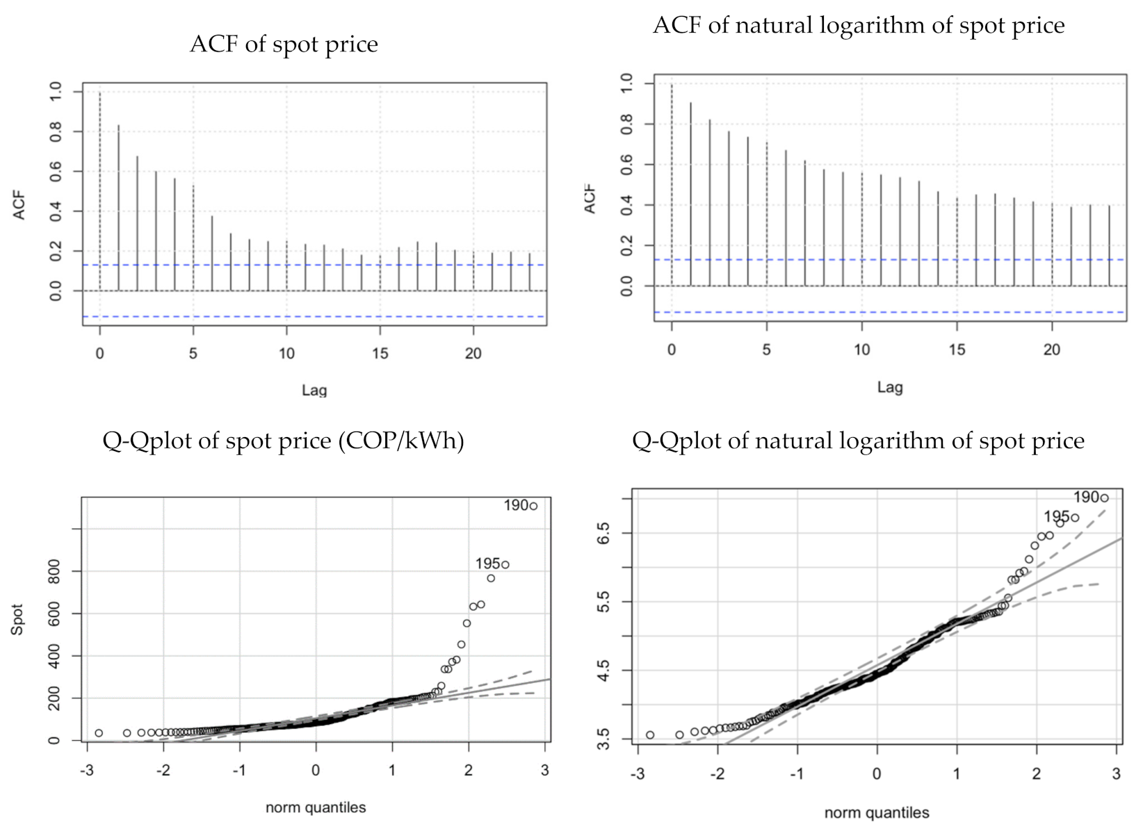
Figure 2 illustrates the spot price series, as well as its autocorrelogram, Q-Qplot, and natural logarithm. There, spot price exhibits a trend and jumps; its highest jump occurs after 2015 due to the occurrence of the El Niño, together with the shortage of natural gas for power generation. The autocorrelograms of spot price and its natural logarithm show the memory condition of this time series. According to the Q-Qplots, which assess the percentiles of the samples, the data do not fit adequately a normal distribution.

ISGG, followed by EPMG and spot price, exhibits the highest level of the first-order autocorrelation, which means that short-term distortions remain for a longer time in these series than in the other ones. Another aspect to highlight is that the skewness changed for the natural logarithm of the series. Regarding dispersion of the series, estimating the percentiles relative to the mean allowed us to observe, for instance, that spot price is between 0.33 times and 2.01 times its mean at a 90% confidence level. After spot price, CHVG is the series with a more extended 90% confidence interval, followed by ISGG, EMPG, and ENDG.

Table 2. Autocorrelation of the series.

Lag	0	1	2	3	4	5	6	7	8	9	10	11	12	13	14
Series
Spot	1.0	0.83	0.68	0.6	0.56	0.53	0.37	0.29	0.26	0.25	0.25	0.23	0.23	0.21	0.18
EPMG	1.0	0.86	0.78	0.73	0.71	0.70	0.68	0.65	0.61	0.59	0.60	0.62	0.62	0.59	0.58
ISGG	1.0	0.88	0.77	0.71	0.69	0.69	0.66	0.62	0.57	0.54	0.55	0.57	0.58	0.52	0.47
CHVG	1.0	0.65	0.29	0.00	−0.16	−0.24	−0.26	−0.26	−0.20	−0.03	0.22	0.39	0.44	0.31	0.12
ENDG	1.0	0.61	0.37	0.23	0.12	0.04	−0.08	0.01	0.15	0.21	0.28	0.35	0.40	0.33	0.19
First differences (Delta of x)
Spot	1.0	−0.03	−0.24	−0.12	0.00	0.35	−0.20	−0.17	−0.06	−0.04	0.05	−0.03	0.05	0.04	−0.09
EPMG	1.0	−0.25	−0.11	−0.14	0.00	0.02	0.05	0.02	−0.05	−0.11	−0.01	0.03	0.13	−0.07	0.08
ISGG	1.0	−0.14	−0.17	−0.16	−0.04	0.12	0.03	−0.01	−0.05	−0.17	−0.05	0.05	0.27	−0.05	−0.11
CHVG	1.0	0.04	−0.09	−0.20	−0.11	−0.07	−0.04	−0.09	−0.18	−0.12	0.11	0.18	0.24	0.10	0.02
ENDG	1.0	−0.19	−0.13	−0.02	−0.06	0.06	−0.27	−0.07	0.11	−0.01	−0.01	0.04	0.15	0.08	−0.07

This tables presents autocorrelation of the series in levels and first differences up to the 14th order.

shows the autocorrelation levels of the time series.

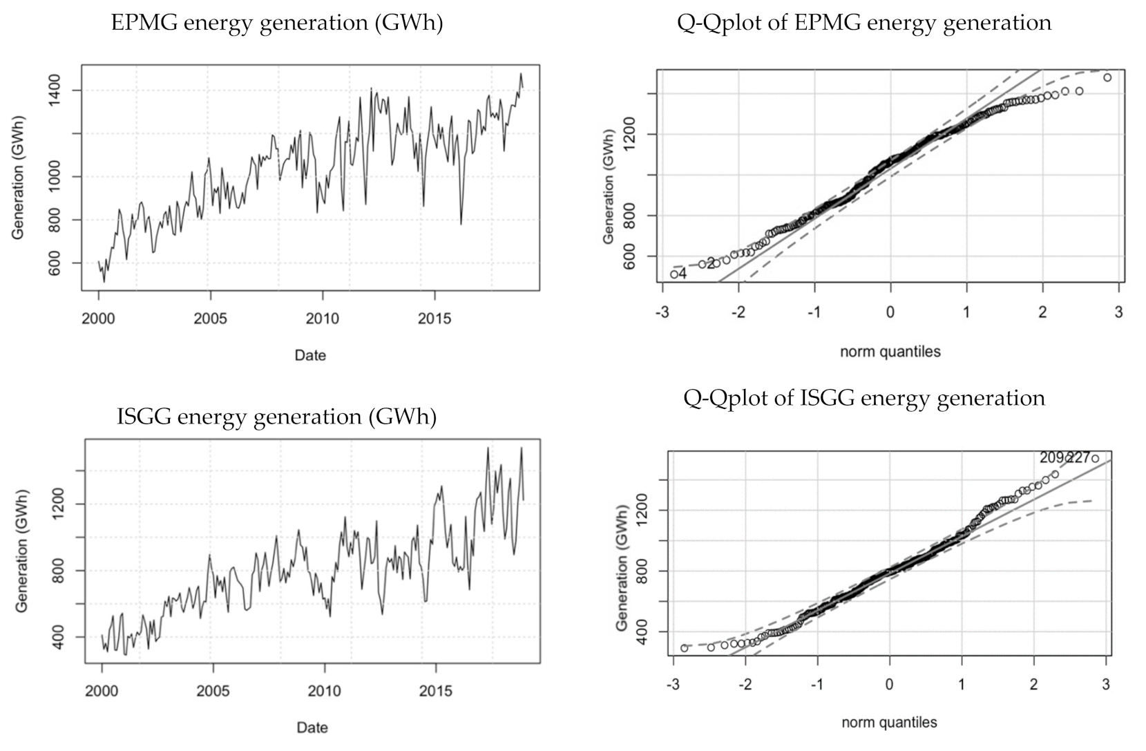
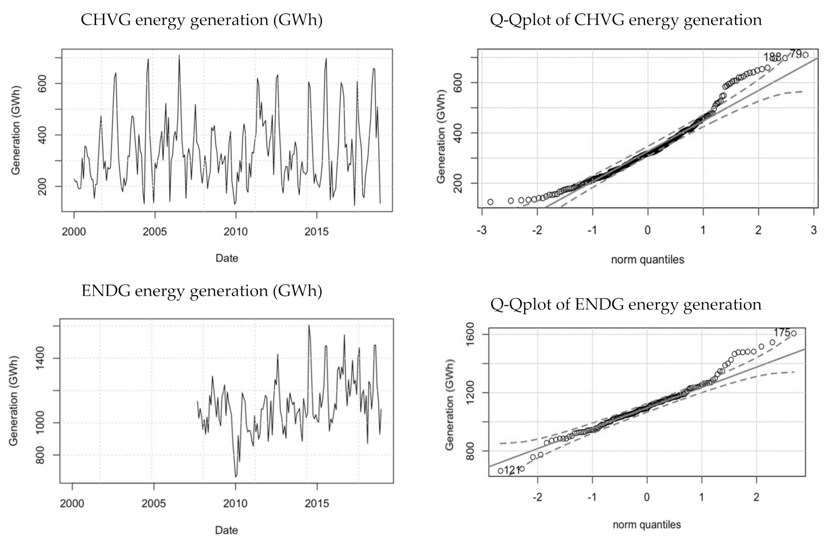
EPMG and ISGG in Figure 3 show a trend explained by the expansion processes of these electricity generators, which have constructed new power plants in recent years. Furthermore, Q-Qplots show how data do not support the normal assumption, particularly at the extremes of the distribution, which calls for the SNP modeling of the series.

4. Results and Discussion

4.1. Parameter Estimation of the Spot Price and Energy Generation Series

Table 3. Estimates for the deterministic trend and AR(1) component of the (log)series.

Parameter		Spot Price	Energy Generation
			EPMG	ISGG	CHVG	ENDG (1)
Beta 0	Coeff	3.84	6.61	6.14	5.68	6.75
	p-value	<0.0001	<0.0001	<0.0001	<0.0001	<0.0001
Beta 1 (2)	Coeff	0.0065	0.0027	0.0043	0.0006	0.0016
	p-value	<0.0001	<0.0001	<0.0001	<0.0001	<0.0001
Phi 1 (3)	Coeff	0.829	0.652	0.673	0.608	0.544
	p-value	<0.0001	<0.0001	<0.0001	<0.0001	<0.0001
Residuals (4)
Statistics	Mean	0.00	0.00	0.00	0.00	0.00
	SD	0.25	0.09	0.15	0.30	0.12
	Skewness	0.51	−0.60	−0.65	−0.43	0.04
	Kurtosis	5.64	4.27	3.76	3.64	3.35
JB test (5)	Statistic	72.1	28.2	21.2	10.6	0.5
	p-value	<0.0001	<0.0001	<0.0001	0.00495	0.77195
	Ho	rejected	rejected	rejected	rejected	Accepted

(1) This series contains information from January 2007. (2) Coefficient of the deterministic trend. (3) Coefficient for the stochastic AR(1) component. (4) Residuals are calculated after a two-stage process in which the trend is fitted first and then the autoregressive component. (5) Jarque–Bera statistic for normality.

presents the parameter estimates of the model in Equations (23) and (24) for the spot price and energy generation series. The model explains the natural logarithm of the series considering a deterministic trend and with AR(1) component; both of them are highly significant. Descriptive statistics for the residuals are also displayed to identify the initial parameters to be considered when estimating the bivariate SNP functions of the series. The Jarque–Bera test is also displayed, revealing the rejection of the normality of the series, except for ENDG.

Table 4. Bivariate SNP fitted distributions of spot price and energy generation.

Epsilon	Descriptive Statistics				Multivariate SNP Estimation (2)
					Standardized Series
Bivariate	Mean	SD	Skewness	Kurtosis		d3	d4	Correlation
Spot Price	0.00	0.25	0.51	5.64	Coeff.		0.166
					p-value		0.001	Coeff.	0.278
EPMG	0.00	0.09	−0.60	4.27	Coeff.	−0.224		p-value	0.106
					p-value	0.002
Spot Price	0.00	0.25	0.51	5.64	Coeff.		0.178
					p-value		<0.0001	Coeff	−0.676
ISGG	0.00	0.15	−0.65	3.76	Coeff.	−0.410		p-value	<0.0001
					p-value	<0.0001
Spot Price	0.00	0.25	0.51	5.64	Coeff.		0.160
					p-value		0.001	Coeff	−0.427
CHVG	0.00	0.30	−0.43	3.64	Coeff.	−0.251		p-value	0.002
					p-value	0.003
Spot Price	0.00	0.25	0.51	5.64	Coeff.		0.146
					p-value		0.023	Coeff	−0.420
ENDG (1)	0.00	0.12	0.04	3.35	Coeff.	−0.041		p-value	0.029
					p-value	0.700

(1) This series was fitted with information from January 2007. (2) SNP expansions include the relevant terms to account for non-normality.

reports the fitted parameters of the bivariate SNP distributions of the vector ${ϵ}_t^i={\left({ϵ}_t^p, {ϵ}_t^{q^i}\right)}^{\prime }$, where the series were filtered from the estimates of the model in the previous stage. As can be inferred from the descriptive statistics, the spot price requires a fourth-order SNP expansion, and parameter d₄ is positive and significant, reflecting the excess kurtosis of this series. However, skewness parameter (d₃) seems not to be relevant and is excluded from the model. On the other hand, the energy generation series exhibit negative and significant skewness, and thus, a third-order SNP is enough to account for non-normality. ENDG series seems to be an exception since, in this case, the coefficient d₃ is not statistically significant, and thus, a normal distribution fits data accurately, as indicated by the Jarque–Bera statistic. The marginal distributions are depicted in Figure A1 of the Appendix B. These plots illustrate how the SNP distributions adequately capture the non-normality of the data. It is also noteworthy that the estimates for marginals are used as initial seeds for the maximum likelihood estimation of the bivariate SNP for every pairwise series.

As far as correlation is concerned, only the distribution of spot price and EPMG has a positive value, although insignificant at a 95% confidence level. The other couples are negative and significant. Note that the level of correlation between ISSG and spot price is higher than that of CHVG-spot price and ENDG-spot price (which are quite similar). These similar correlation levels may be explained by the close geographical location of two dams with similar generation capacity between these two electricity generators.

The scatterplots in Figure 4 compare the residuals of spot price, ${ϵ}_t^p$, with those of each energy generation, ${ϵ}_t^{q_i}$, to illustrate the co-movements among these variables. Fitted lines capture the linear correlation among the variables. Furthermore, the figures for both bivariate pdf and cumulative distribution function (cdf) of the spot price and energy generation series can be found in Figure A2 in Appendix B.

4.2. Sensitivity of the Risk Indicators

This subsection shows an example of the performance of the SNP model for risk management in forward contracts in Colombian energy markets. For this purpose, we discuss the behavior of the risk indicators at different values of the forward contracting level (Eta), the FRP and the correlation (Rho). The sensitivity analyses performed in this study correspond to simulations based on a hypothetical generator’s portfolio. Consistently with the values calibrated for the series, this portfolio is characterized by having a mean and standard deviation of ${ϵ}_t^{q_i}$ of 1 and 0.09133, respectively. In addition, it follows a third-order SNP distribution, with coefficient $d_3$ equal to −0.07415 and a correlation between the transformed components of spot price and energy generation of −17%. For the spot price, we consider the parameters estimated for the Colombian electricity market (see Table 3 and Table 4), which are the conditions that a hypothetical generator would be facing. A thousand simulations were conducted for the Monte Carlo method.

Eta $\left(\eta \right)$ captures the portion of the expected energy generation that is sold through forward contracts. For instance, if an electricity generator is expected to produce an average of 100 GWh of electricity in a specific time and its Eta is 0.9, it will be selling 90 GWh through a long-term contract. If this generator produced 110 GWh at maturity, it would have sold 90 GWh through the forward contract at a known price; and 20 GWh at the spot price. In the event that it had sold 90 GWh in the contract but only generated 80 GWh at maturity, it would have to procure the remaining 10 GWh from the spot market to meet its obligations.

Figure 5 illustrates the behavior of the mean and the standard deviation of the hypothetical generator’s portfolio at different Eta and FRP values. From this figure, we observe that when the FRP value is zero (forward price is equal to the expected spot price), the mean of the net income from energy sales will remain constant and does not depend on the Eta. The standard deviation depends on the Eta; the curve of the standard deviation is convex. Unlike the mean of the portfolio, the curve of its standard deviation does not change at different FRP values.

Increasing Eta when the FRP value is negative will result in higher expected sales, as shown in Figure 6 when the FRP value is −5, −10, and −20. Based on this, it is, thus, clear that the more negative the FRP value, the higher the expected value for the electricity generator when it increases its forward contracting level. Conversely, the more positive the FRP value, the lower the expected income.

Figure 6 shows the behavior of the VaR and CVaR curves at different Eta values, which differ from those of the standard deviation. We observe that the CVaR is consistently lower than the VaR and maintains a smoother behavior than the distortions that the latter seems to have. Additionally, the CVaR curve increases faster than that of the VaR once the Eta value exceeds its maximum value. This situation occurs due to the thickening of the income’s left tail when the generator must procure the forward contract quantity by buying at spot market.

When the Eta values are positive, a negative FRP involves a better risk condition for the electricity generator. To improve the mean and the left-tail risk indicators, the generator will always prefer to sell at a higher forward price. Furthermore, variations in the FRP also seem to move the maximum point of the indicators, as shown in Figure 7. For instance, if an electricity generator considers that it is optimal to sell a number of contracts equal to 75% of its expected energy generation under a FRP value of zero, the optimal Eta value will change if the FRP value drops to −10. Therefore, the optimal forward contracting level depends not only on the uncertainty conditions of the spot price and the energy generation but also on market conditions and the way the market values the assumed risk levels.

Moreover, the correlation between spot price and energy generation affects the optimal decision. Figure 8—constructed assuming an FRP equal to zero—presents the behavior of the risk indicators under analysis at different correlation values. A positive correlation tends to increase the optimal contracting level. In contrast, a negative one tends to reduce it, which is consistent with the belief that a negative correlation represents a natural hedge. Another perceived effect is that the VaR and CVaR levels rise as the correlation values increase: a positive correlation shows a higher CVaR value than a negative one.

4.3. Effect of SNP Parameters

In this section, we present the sensitivity of the CVaR and the contracting level (Eta) at different d₃ and d₄ values for the hypothetical generator’s energy generation. The first graph of Figure 9 plots the behavior of the CVaR when the marginal distribution of the energy generation only contains the third-order HP, and parameter d₃ takes values of 0.5, 0.14, 0.07, 0, −0.07, and −0.14. The second graph shows a similar sensitivity analysis, but for the fourth-order HP. It is worth noting that d₃ = 0, and d₄ = 0 indicates a normal distribution.

The d₃ and d₄ coefficients affect the CVaR. If we take the case of a normal distribution as a reference, negative coefficients tend to decrease the CVaR levels, while positive ones tend to increase them and move the maximum point to the right. Normal conditions do not allow us to properly represent the sensitivity of risk indicators to different hedging levels.

4.4. Optimal Forward Contracting Level

Table 5. Optimal contracting level (Eta) suggested for each generator.

FRP	EPMG				ISGG
	Mean (1)	SD	VaR	CVaR	Mean	SD	VaR	CVaR
−20	2	1.13	1.20	0.96	2	0.61	0.62	0.49
−15	2	1.13	1.16	0.95	2	0.61	0.62	0.48
−10	2	1.13	1.16	0.95	2	0.61	0.61	0.48
−5	2	1.13	1.16	0.95	2	0.61	0.56	0.46
−2	2	1.13	1.16	0.95	2	0.61	0.56	0.45
0	0	1.13	1.06	0.93	0	0.61	0.56	0.43
2	0	1.13	1.04	0.90	0	0.61	0.44	0.43
5	0	1.13	1.04	0.85	0	0.61	0.44	0.41
10	0	1.13	1.00	0.83	0	0.61	0.26	0.40
15	0	1.13	0.95	0.76	0	0.61	0.26	0.40
20	0	1.13	0.95	0.76	0	0.61	0.24	0.40
FRP	CHVG				ENDG
	Mean	SD	VaR	CVaR	Mean	SD	VaR	CVaR
−20	2	0.88	0.81	0.67	2	0.87	0.84	0.74
−15	2	0.88	0.81	0.66	2	0.87	0.84	0.73
−10	2	0.88	0.81	0.66	2	0.87	0.84	0.72
−5	2	0.88	0.79	0.65	2	0.87	0.77	0.72
−2	2	0.88	0.69	0.64	2	0.87	0.76	0.71
0	0	0.88	0.69	0.64	0	0.87	0.76	0.71
2	0	0.88	0.69	0.64	0	0.87	0.76	0.71
5	0	0.88	0.69	0.63	0	0.87	0.76	0.7
10	0	0.88	0.69	0.63	0	0.87	0.76	0.69
15	0	0.88	0.69	0.62	0	0.87	0.76	0.67
20	0	0.88	0.68	0.61	0	0.87	0.68	0.66

(1) The simulation was performed using Eta values between 0 and 2. In the case of the mean, the Eta optima occur at a corner solution.

reports the optimal hedge levels suggested for each electricity generator under study at different FRP values and different optimization criteria. Parameter estimation for each agent was performed for all available monthly data from 2000 to 2018. For the mean, the VaR, and the CVaR criteria, we considered the contracting level that maximizes each of them, and for the standard deviation, the contracting level that minimizes it. The contracting level that minimizes the standard deviation of the portfolio depends on the particular conditions of each electricity generator and not on the market conditions (FRP). In general, the suggested contracting levels are below one, except for EPMG, which is required to increase its forward sales, possibly because this generator has positive correlation levels higher than those of the other three generators under analysis.

Moreover, for all generators, we observede that the negative FRP values tendd to increase the optimal Eta for the VaR and the CVaR indicators. In particular, based on the sensitivity analyses performed, the optimal Eta can reach variations up to 15%. According to Table 5, the contracting level obtained for EPMG using the VaR is on average 10% higher than that obtained with the CVaR. In the case of ISGG, we observed that the suggested contracting levels were clearly lower than those of the other electricity generators. This situation may be explained by the fact that the unexplained component of the ISGG series exhibits a negative correlation higher than that of the other generators. A positive correlation tends to increase the contracting levels, while a negative one tends to reduce them.

We found that the hedge ratio depended on several conditions, some of them linked to the market situation, as the estimated FRP or the frequency function governing the uncertainty sources; others concerned to the agent, as the production or the decision-making criteria. For the same agent at the same FRP conditions, the optimal hedge ratio depends on the risk measure to be considered. Therefore, in order to create a static hedge strategy, policy makers should be aware of the need for implementing all the estimation and simulation methods suggested in this research.

5. Conclusions

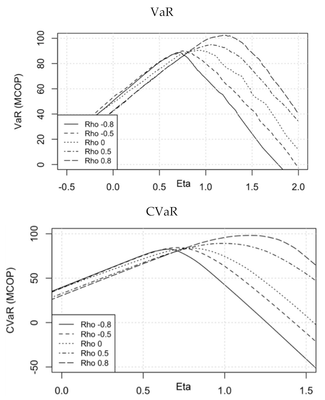
This paper proposes a static hedging strategy for electricity generators that participate in a competitive market where hedging is carried out through forward contracts that include a risk premium in their valuation. We considered the spot price and energy generation variables to follow a bivariate SNP distribution defined in terms of the Gram–Charlier (Type A) expansion. This distribution allowed us to not only model the mean, the variance, and their correlation but also the skewness, the kurtosis, and higher-order moments. Moreover, we used Monte Carlo simulation to analyze the effect of three risk indicators (standard deviation, VaR, and CVaR) on the net profit from energy sales, using information from the Colombian electricity market as the case study. We found that positive correlation between the spot price and energy production tends to increase the hedge ratio; meanwhile, negative correlation tends to reduce it.

This work’s main contribution is the modeling and analysis of the risk faced by electricity generators through flexible SNP multivariate distributions, as well as the structuring of a hedging portfolio that does not impose the assumption of normality on price and energy generation, which is a novelty in this academic field, where, as far as we know, multivariate semi-nonparametric technics have been used before. The performance of the model for implementing forward contracts hedging strategies is assessed though the Monte Carlo simulation of bivariate SNP pdfs and by studying the sensibility of risk measures to the different parameters affecting forward electricity markets.

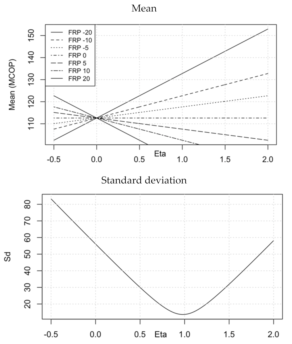
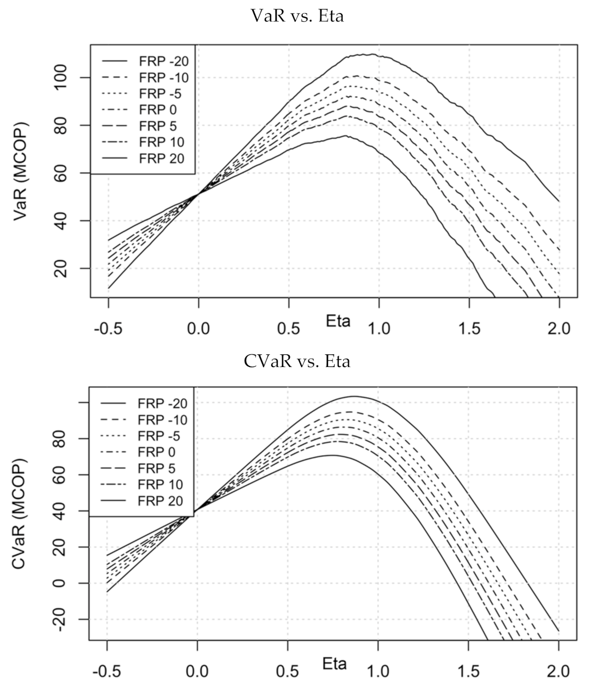
In general, a negative FRP increases an electricity generator’s net profit from its energy sales in the contract market, thus, favoring electricity forward sales. Moreover, the FRP affects the behavior of the mean, VaR, and CVaR indicators regarding the amount of electricity to be sold under forward contracts. This situation does not occur for the standard deviation, whose behavior, instead, is affected by the contracting level, regardless of the FRP value in the market.

The results show that the optimal quantity of energy to be sold through forward contracts is dependent not only on the conditions of spot price and quantity uncertainty but also on the way market agents weigh the assumed risk levels. Therefore, to reduce the risk levels faced by generators, such optimal quantity will depend on the conditions of price and energy generation uncertainty explained by variance, skewness, kurtosis, and higher-order moments. Furthermore, the number of forward sales is determined by the correlation between price and energy generation and the FRP, or an increment on correlation or FRP, tends to reduce the hedge ratio.

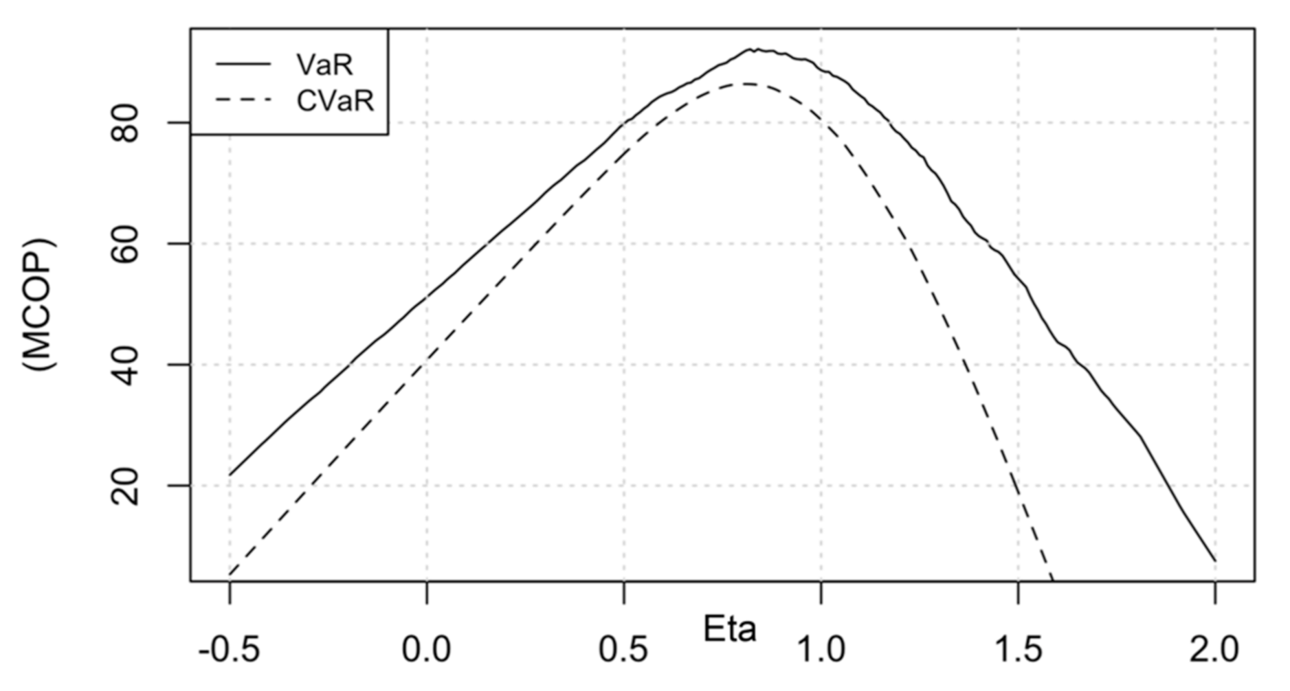
The decision-making criteria also modify the optimal hedge ratio. The VaR-maximization criterion implies a larger hedge ratio than the CVaR-maximization criterion; this criteria selection could have more impact on the optimal decision than the FRP modifications. It suggests that electricity market practitioners must pay significant attention to market conditions and the adequate risk measures that accomplish each business strategy. It is necessary to find coherence among strategy, risk aversion, and risk retention capacity.

All in all, we recommend experts in electricity markets to structure company-specific portfolios based on the market conditions on which the analysis is performed. They should also consider flexible modeling that captures a more significant number of moments than those allowed by a normal distribution for the variables involved and the correlation between the spot price and energy generation. The multivariate SNP distribution can be an appropriate tool for this purpose. As a final remark, although this work is done for a hydropower-dominated market, the convenience of this methodology for other electricity markets should be studied for further works.

References

1. Mosquera-López, S.; Uribe, J.M.; Manotas-Duque, D.F. Nonlinear empirical pricing in electricity markets using fundamental weather factors. Energy 2017, 139, 594–605. [Google Scholar] [CrossRef]
2. Alqurashi, A.; Etemadi, A.H.; Khodaei, A. Treatment of uncertainty for next generation power systems: State-of-the-art in stochastic optimization. Electr. Power Syst. Res. 2016, 141, 233–245. [Google Scholar] [CrossRef]
3. Pilipovic, D. Energy Risk, Valuing and Managing Energy Derivatives; McGraw-Hill: New York, NY, USA, 2007. [Google Scholar]
4. Weron, R. Electricity price forecasting: A review of the state-of-the-art with a look into the future. Int. J. Forecast. 2014, 30, 1030–1081. [Google Scholar] [CrossRef] [Green Version]
5. Ciupageanu, D.A.; Barelli, L.; Lazaroiu, G. Real-time stochastic power management strategies in hybrid renewable energy systems: A review of key applications and perspectives. Electr. Power Syst. Res. 2020, 187, 106497. [Google Scholar] [CrossRef]
6. Woo, C.-K.; Karimov, R.; Horowitz, I. Managing electriciry procurement cost and risk by a local distribution company. Energy Policy 2004, 32, 635–645. [Google Scholar] [CrossRef]
7. Nässäkkälä, E.; Keppo, J. Electricity Load Pattern Hedging with Static Forward Strategies. Manag. Financ. 2005, 31, 116–137. [Google Scholar] [CrossRef] [Green Version]
8. Oum, Y.; Oren, S.S. Optimal Static Hedging of Volumetric Risk in a Competitive Wholesale Electricity Market. Decis. Anal. 2010, 7, 107–122. [Google Scholar] [CrossRef] [Green Version]
9. Boroumand, R.; Goutte, S.; Porcher, S.; Porcher, T. Hedging strategies in energy markets: Te case of electricity retailers. Energy Econ. 2015, 51, 503–509. [Google Scholar] [CrossRef]
10. Longstaff, F.; Wang, A. Electricity Forward Prices: A High-Frequency Empirical Analysis. J. Financ. 2004, 59, 1877–1900. [Google Scholar] [CrossRef] [Green Version]
11. Xiao, Y.; Colwell, D.; Ramaprasad, B. Risk Prem. in Electricity Prices: Evidence from the PJM Market. J. Futures Mark. 2014, 35, 776–793. [Google Scholar] [CrossRef]
12. Botterud, A.; Kristiansen, T.; Ilic, M. The relationship between spot and futures prices in the Nord Pool electricity market. Energy Econ. 2010, 32, 967–978. [Google Scholar] [CrossRef]
13. Pantoja, J. Modelling risk for electric power markets. (eafit, Ed.). Innovar 2012, 22, 51–66. [Google Scholar]
14. Redl, C.; Bunn, D. Determinants of the premium in forward contracts. J. Regul. Econ. 2013, 43, 90–111. [Google Scholar] [CrossRef]
15. Bunn, D.; Chen, D. The forward premium in electricity futures. J. Empir. Financ. 2013, 23, 173–186. [Google Scholar] [CrossRef]
16. Ruddell, K.; Downward, A.; Philpott, A. Market power and forward prices. Econ. Lett. 2018, 166, 6–9. [Google Scholar] [CrossRef] [Green Version]
17. Trespalacios, A.; Rendón, J.F.; Pantoja, J. Estrategia de cobertura a través de contratos a plazo en mercados eléctricos. Acad. Rev. Latinoam. Adm. 2012, 50, 148–157. [Google Scholar]
18. Trespalacios, A.; Cortés, L.; Perote, J. Uncertainty in electricity markets from a semi-nonparametric approach. Energy Policy 2020, 137, 111091. [Google Scholar] [CrossRef]
19. Brunner, A.D. Conditional asymmetries in real GNP: A Seminonparametric Approach. J. Bus. Econ. Stat. 1992, 10, 65–72. [Google Scholar]
20. Gallant, A.R.; Nychka, D.W. Seminonparametric maximum likelihood estimation. Econometrica 1987, 55, 363–390. [Google Scholar] [CrossRef] [Green Version]
21. Mauleon, I.; Perote, J. Testing Densities with Financial Data: An Empirical Comparison of the Edgeworth-Sargan density to the Student’st. Eur. J. Financ. 2000, 6, 225–239. [Google Scholar] [CrossRef]
22. Cortes, L.M.; Mora-Valencia, A.; Perote, J. The productivity of top researchers: A semi-non-parametric approach. Scientometrics 2016, 118, 891–915. [Google Scholar] [CrossRef] [Green Version]
23. Cortés, L.M.; Mora-Valencia, A.; Perote, J. Measuring firm size distribution with semi-nonparametric densities. Phys. A 2017, 485, 35–47. [Google Scholar] [CrossRef]
24. Perote, J. The multivariate Edgeworth-Sargan density. Span. Econ. Rev. 2004, 6, 77–96. [Google Scholar] [CrossRef]
25. Ñíguez, T.M.; Perote, J. The Multivariate Moments Expansion Density: An Application of the Dynamic Equicorrelation Model. J. Bank. Financ. 2016, 72, S216–S232. [Google Scholar] [CrossRef] [Green Version]
26. Del Brío, E.B.; Mora-Valencia, A.; Perote, J. The kidnapping of Europe: High-order moments’ transmission between developed and emerging markets. Emerg. Mark. Rev. 2017, 31, 96–115. [Google Scholar] [CrossRef]
27. Ñíguez, T.M.; Perote, J. Forecasting Heavy-Tailed Densities with Positive Edgeworth and Gram-Charlier Expansions. Oxf. Bull. Econ. Stat. 2012, 74, 600–627. [Google Scholar] [CrossRef]
28. Jondeau, E.; Rockinger, M. Gram-Charlier densities. J. Econ. Dyn. Control 2001, 25, 1457–1483. [Google Scholar] [CrossRef]
29. Del Brio, E.B.; Ñíguez, T.M.; Perote, J. Gram-Charlier Densities: A Multivariate Approach. Quant. Financ. 2009, 9, 855–869. [Google Scholar] [CrossRef] [Green Version]
30. Bessebender, H.; Lemmon, M. Equilibrium Pricing and Optimal Hedging in Electricity Forward Markets. J. Financ. 2002, 57, 1347–1382. [Google Scholar] [CrossRef]
31. Hull, J.C. Options, Futures and Other Derivatives; Pearson, Prentice Hall: London, UK, 2009. [Google Scholar]
32. Lucia, J.J.; Schwartz, E.S. Electricity prices and power derivatives: Evidence from the nordic power exchange. Rev. Deriv. Res. 2002, 5, 5–50. [Google Scholar] [CrossRef]
33. Geman, H.; Roncoroni, A. A Class of Marked Point Processes for modelling Electricity Prices; ESSEC Working Papers; DR 03004; ESSEC Research Center, ESSEC Business School: Cergy, France, 2003; pp. 2–70. [Google Scholar]
34. Uribe, E.; Trespalacios, A. Contraste de modelos estocásticos para el precio de la energía en Colombia. Factultad Cienc. Univ. Nac. Colomb. 2014, 3, 41–55. [Google Scholar]
35. Del Brio, E.B.; Ñíguez, T.M.; Perote, J. Multivariate SNP Distributions with Dynamic Conditional Correlations. Int. J. Forecast. 2011, 27, 347–364. [Google Scholar] [CrossRef]
36. Fusai, G.; Roncoroni, A. Implementing Models in Quantitative Finance: Methods and Cases; Springer Finance: New York, NY, USA, 2008. [Google Scholar]
37. Meucci, A. Risk and Asset Allocation; Springer: New York, NY, USA, 2007. [Google Scholar]
Figure 1. Monte Carlo simulation of bivariate distribution. This figure illustrates the method used to simulate random numbers based on [33].
Energies 14 03345 g001
Figure 2. Spot price time series of energy in Colombia. The Q-Q plots of the spot price and of its natural logarithm are compared to the normal distribution at a 95% confidence interval.
Energies 14 03345 g002aEnergies 14 03345 g002b
Figure 3. Energy generation time series of different electricity generators in Colombia. The Q-Qplots of the energy generation are compared to the normal distribution at a 95% confidence interval.
Energies 14 03345 g003aEnergies 14 03345 g003b
Figure 4. Scatterplots of the residuals of spot price versus those of each energy generation. Linear correlations among the variables is depicted with the fitted lines.
Energies 14 03345 g004
Figure 5. Sensitivity of the mean and the standard for Eta and FRP. Simulation of the behavior of the mean and standard deviation at different contracting levels (Eta) and forward risk premium (FRP).
Energies 14 03345 g005
Figure 6. Sensitivity of the VaR and the CVaR to the contracting level (Eta). Simulation of the behavior of the value-at-risk (VaR) and conditional VaR (CVaR) at different contracting levels (Eta).
Energies 14 03345 g006
Figure 7. Sensitivity of the VaR and the CVaR to the Eta and FRP. Sensitivity of the value-at-risk (VaR) and conditional VaR (CVaR) to different contracting levels (Eta) and forward risk premium (FRP) values.
Energies 14 03345 g007
Figure 8. Sensitivity of the standard deviation, the VaR, and the CVaR to the Eta and Rho. Sensitivity of the standard deviation, the value-at-risk (VaR), and the conditional VaR (CVaR) of the net income from the sale of energy to different contracting levels (Eta) and correlation values (Rho).
Energies 14 03345 g008aEnergies 14 03345 g008b
Figure 9. Sensitivity of the CVaR to different SNP parameters. Sensitivity of the conditional value-at-risk (CVaR) to skewness (d3) and kurtosis (d4) parameters. The y axis in both graphs is measured in million Colombian pesos (MCOP).
Energies 14 03345 g009