
Real Fault Location in a Distribution Network Using Smart Feeder Meter Data


1
Clinical-Laboratory Center of Power System & Protection, Faculty of Intelligent Systems Engineering and Data Science, Persian Gulf University, Bushehr 75169113817, Iran
2
Kamstrup A/S, Industrivej 28, DK-8660 Stilling, Skanderborg, Denmark
3
Center for Energy Informatics, University of Southern Denmark, DK-5230 Odense, Denmark
*
Authors to whom correspondence should be addressed.
Energies 2021, 14(11), 3242; https://doi.org/10.3390/en14113242
Submission received: 11 May 2021
/
Revised: 24 May 2021
/
Accepted: 26 May 2021
/
Published: 1 June 2021
(This article belongs to the Collection Featured Papers in Electrical Power and Energy System)
Abstract
:Distribution networks transmit electrical energy from an upstream network to customers. Undesirable circumstances such as faults in the distribution networks can cause hazardous conditions, equipment failure, and power outages. Therefore, to avoid financial loss, to maintain customer satisfaction, and network reliability, it is vital to restore the network as fast as possible. In this paper, a new fault location (FL) algorithm that uses the recorded data of smart meters (SMs) and smart feeder meters (SFMs) to locate the actual point of fault, is introduced. The method does not require high-resolution measurements, which is among the main advantages of the method. An impedance-based technique is utilized to detect all possible FL candidates in the distribution network. After the fault occurrence, the protection relay sends a signal to all SFMs, to collect the recorded active power of all connected lines after the fault. The higher value of active power represents the real faulty section due to the high-fault current. The effectiveness of the proposed method was investigated on an IEEE 11-node test feeder in MATLAB SIMULINK 2020b, under several situations, such as different fault resistances, distances, inception angles, and types. In some cases, the algorithm found two or three candidates for FL. In these cases, the section estimation helped to identify the real fault among all candidates. Section estimation method performs well for all simulated cases. The results showed that the proposed method was accurate and was able to precisely detect the real faulty section. To experimentally evaluate the proposed method’s powerfulness, a laboratory test and its simulation were carried out. The algorithm was precisely able to distinguish the real faulty section among all candidates in the experiment. The results revealed the robustness and effectiveness of the proposed method.
1. Introduction
Electricity distribution networks are mainly responsible to transfer electricity from the upstream network (transmission networks) to domestic, commercial, or small industry customers, with good quality. Conditions and events such as the depreciation of distribution network equipment (lines, insulators, etc.) and unfavorable weather conditions such as lightning, falling trees, or external objects on the network lines, cause faults and consequently lead to inevitable power outages [1]. Therefore, faults may occur in the distribution network with different resistances and types (single-, two-, three-phase to ground fault) at different locations of the network, based on the fault circumstances and conditions [2]. On the other hand, power outages cause customer dissatisfaction, financial losses, and reduced reliability. Hence, it is necessary to provide a method that can quickly and accurately locate fault points in the distribution network, independent of its conditions. FL methods are mainly a part of the following categories:
Traveling wave-based methods apply high sampling-rate devices and the speed of the wave in the electricity line to determine the fault point in the network. A comprehensive review of traveling wave-based FL algorithms for power networks, with the high-penetration distributed generations is presented in [7]. In [8], a traveling wave-based FL algorithm is presented for distribution networks, which employ decomposition of the variational mode and the operator of Teager energy.
First, before fault occurrence, according to the network topology and the characteristic of the wave scattering, the inherent distance difference matrix is created. After a fault occurs, a new fault distance difference matrix is generated with the help of fault traveling waves arrival time and double-ended traveling wave algorithm. To completely support all sections of the network, it is vital to install high sampling-rate devices at the end of all last sections of the network. This means that every single node that is connected to the network with only one line, needs a measurement. Note that in this method, all measuring devices must record the waveform of voltage and current. The method needs high sampling-rate devices.
The accuracy of the method may dramatically decrease for those networks with smaller distances between nodes because of the wave speed in the network. Many existing branches and sub-branches and junction points in the distribution network make the FL procedure a challenging task. Therefore, the authors of [9] proposed a new method to precisely locate the fault distance in multiple-branch distribution networks, by utilizing the traveling waves of the circuit breaker reclosure-generation. To calculate the distance of the fault, the reflected traveling wave arrival time of the fault point and the reclosing instant are employed. In this method, an offline data bank is used to distinguish the real location of the fault from the rest due to the fault occurrence possibility in the network branches and sub-branches. This data bank includes reclosure-generating traveling waves of fault for each section. After all possible sections are determined by the algorithm, the real fault wave is compared to all data bank waves. The most similar wave represents the real section of the fault. This method’s drawback is that it needs an accurate data bank, which decreases its application in the real-world distribution networks because of their uncertainty.
In [10], a new traveling wave-based method is presented to locate the grounding faults in the power system. The main idea comes from the difference between the time of arrival of the aerial and grounded mode traveling waves. The frequency-dependent ingredients of power systems consider the grounded mode waves as a variable and the aerial mode as a constant. The least-squares method is applied to solve the pre-determined quadratic function, which is created on the basis of the relation between fault distance and wave speed for each line, separately. The boundary of fault distance is calculated by comparing the minimum and maximum values of the grounded mode speeds. Afterward, the accurate location of the fault is determined using iterative calculation. This method needs high sampling-rate devices and has a higher complexity, as compared to the impedance-based methods.
In [11], a new FL method is proposed for a distribution network. The method uses a synchronized traveling wave detector. In this work, the effect of electrical network ingredients, on the propagation of the traveling wave is also investigated. This method needs a high sampling-rate synchronized device for satisfactory performance. A simple and applicable method is presented in [12] to locate faults in a multi-branch distribution network. This method uses traveling waves and their reflections of several independent and not necessarily synchronous measurements, which are located on a single end of a network. The DGs penetrations, multiple branches of distribution networks, and the arrival time errors adversely affect the FL methods. Therefore, in [13], a new clustering traveling wave-based FL method is presented to overcome such difficulty. An optimization model is defined for each section of the network, based on the traveling wave arrival time. The sum of the square error minimization function is introduced with respect to fault distance and wave velocity. The particle swarm optimization algorithm which is a population-based optimization method is utilized, because of the stochastic nature of the problem. The wide area traveling wave FL method is presented in [14]. This method has two steps for determining the area of fault and the accurate fault distance in the faulty domain using high sampling-rate synchronous measurements, which restricts its real-world application. In [15], an FL algorithm is presented, which applies the traveling wave–time frequency characteristics. The exact location of the fault could be computed using the location formula of the modulus wave speed difference. This method only locates single-phase ground faults.
Machine learning-based FL algorithms as a family member of intelligent methods are some highly popular procedures for determining fault points in distribution networks, with the least available information. In [16], the machine-learning application on fault classification and location in radial electrical networks is investigated. In this work, first, the recorded current signal is fed to a discrete wavelet transform decomposition for extracting the main features. Then a multi-layer perception (MLP) is utilized to detect if the fault has happened in the network or not. MLP is among the group of feed-forward artificial neural networks. In the next step, the fault is classified using MLP. Finally, by employing MPL or extreme learning machine (ELM), the location of fault is estimated. Note that, in this work, it is vital to train the models with rich enough data, which is extracted from the network, to obtain the accurate parameters of the models.
In [17], a new machine-learning-based approach is presented to locate the fault in the distribution grids, which uses decomposed upstream recorded current (by passing through wavelet transform) to collect applicable features. All collected data are fed to ELM for the learning process. Support vector regression and artificial neural network are also applied. The results revealed that ELM operates better in terms of performance and training time. This method is complex and needs rich enough data for the training step. In [18], an adaptive convolution neural network-based FL algorithm is proposed for a two-terminal distribution network. This method improves the ability of feature extraction and has a superior performance, as compared to the deep belief network.
In [19], a new artificial neural network-based FL method is presented for the radial distribution network. Pre- and post-fault current profiles are used to train an artificial neural network model to identify and locate short circuit faults. The main drawback of this method is that it needs to be trained at any circumstances of the network, which increases the complexity, and as a result lowers the accuracy. The authors of [20], have proposed a new FL method for identifying the faulty section of distribution grids, using Stockwell transform, to extract features from the fault currents. The features are fetched as inputs to several intelligent methods such as MLP-neural network, support vector machine, and ELM. The main parameters of intelligent methods have been optimized using a constriction factor particle swarm optimization algorithm. This method needs a data bank for the training process. Support vector machine as one of the most common machine learning methods is a strong tool for locating faults in distribution networks.
In [21], the support vector machine-based FL method has been presented for distribution grids that use discrete wavelet transform to convert the raw current signal for the feature extraction process. In [22], the faulty branch and fault distance are determined using the support vector machine and similarity matching methods. In [23], traveling-wave frequencies and ELM are employed to determine the location of a fault in the transmission line. First, the time-domain transient data of fault turn into the frequency domain for detecting the frequencies of the traveling wave. The initial location of the fault is estimated using this information. Finally, ELM is utilized to locate the accurate location of the fault.
State estimation-based FL methods are good options for avoiding the use of complex methods with heavy calculation burdens, which need a databank and accurate topology of network, with mostly known load values [24]. In [25], a new state estimation-based method was suggested for determining the location of a fault in a distribution network equipped with SMs. The FL procedure has been carried out by defining the concept of bad data as a location of the fault in the network—which can be considered to be a temporary load connected to the network—and determining its place with the use of weighting matrix bad data identification approach. This method is robust against measurements error and does not need the type of fault, but it needs adequate measuring devices in the network that make it fully observable. By advancing the technology, the use of phasor measurement units (PMUs) in the distribution networks has increased significantly.
In the recent research work [26], a new state-estimation-based FL method is proposed, which can detect and locate short circuit faults in active distribution networks. It uses the revised state estimation and pre-fault state estimation results, as well as the recorded post-fault voltage and current to detect the faulty section. The procedure consists of two main steps—the first step involves diagnosing the faulty zone and the second step involves detecting the fault section. This method as the work of [25], needs a specific number of measurements and is unable to locate the exact FL in the section. In [27], a new PMU-based state estimation method is presented to detect and identify the fault section of active distribution networks. In this method, the fault in the network can be detected using a real-time process. For the functionality of this method, it is vital to use adequate synchronous measurements in certain locations of the network to guarantee the network’s full observability. The faulty section can be specified by considering the faulty point as a floating bus and generating new parallel state estimators, using the augmented topology of the network. The state estimation-based FL method can also operate well under high penetration photovoltaic DGs [28]. Spare measurements can be useful for FL procedures.
In [29], a new iterative state-estimation-based method is presented to detect the faulty line. This method has two steps. First, it uses a state estimation method in an iterative manner to determine the nearest bus to the fault point. Second, by examining all connected sections to the identified node, the faulty section can be specified. In [30], a new state estimation wide-area FL is presented. This method can also identify the faulty phase and its type. A new extended and modified version of the state-estimation method with weighted least squares is used to decrease the effect of measurement error. High impedance faults have low fault current, which makes the FL procedure a challenging task. In [31], a state-estimation-based method is proposed for detecting and locating the high-impedance faults in the distribution networks. FL and fault detection formulation for both and line models are provided. In this work, it is necessary to have adequate measurement in the network.
Impedance-based methods use phase-domain recorded information, instead of time-domain ones, which makes the FL procedure more cost-effective than complex methods such as the intelligent and traveling wave methods. In [32], a new high-frequency impedance-based method is presented to locate a fault in the distribution networks. High frequency measuring components are used to avoid the effect of controlling systems on the FL procedure. This method needs enough measurements to support all sections of the network. Phase-domain information of fault current and voltage is used in impedance-based methods [33]. The authors of [34] proposed a new adaptive impedance-based method to locate faults in active distribution networks, using the recorded phase-domain voltage and current. The detailed model of distributed energy resources is used to accurately estimate its contribution to the fault current. In this work, a real faulty section cannot be identified in multi-lateral networks. Using the distributed line model of the network in FL procedure increases the accuracy and reduces the error percentage [35]. In [36], a new method is presented to locate faults in double circuit distribution networks. In this work, distributed line parameters are used to enhance the accuracy of FL. The recorded pre- and post-fault data at the substation are adequate for the FL procedure. Reference [37] presents a new improved impedance-based FL for distribution networks, using distributed line parameters (DLPs). Two types of fifth-order algebraic formulas are obtained for short circuit and phase to phase faults. This method only uses the substation recorded current and voltage and the accurate load value of each node. The proposed method may give several fault points for those networks, with many laterals. The same authors in [38], solve the drawback of [37] by proposing a new frequency spectrum analysis method to differentiate between the real FL and the remaining candidates. In [39], a new FL method is suggested for the smart distribution networks that utilizes present and historic recorded data of SMs as well as micro-PMUs. Since impedance-based methods need the load data of each node of the network, this work presents a new algorithm to estimate the load value at fault-time occurrences. Reference [17] also suggests a simple least square error-based section estimation method to determine the real location of fault among all candidates.
In this paper, a new impedance-based method is presented to determine the real fault section using SFMs data. The proposed method does not require high-resolution measurements, which is among the main advantage of the method. First, the last pre-fault recorded active and reactive power by SMs in the low voltage side of the network. Additionally, the recorded voltage and current at the substation are fed to a load-flow algorithm to determine the voltage of each node and subsequently load their impedance value. Then, the equivalent load impedance (ELI) at the end of each section is calculated, using the circuit theory and Ohm’s law. By running the FL algorithm, all possible solutions of FL are accomplished. Afterward, the proposed section estimation algorithm, which uses the post-fault recorded active power, detects the real section of the fault. After the protection relay detects a fault in the network, it sends a pulse to all SFMs to instantaneously record the active power of their connected lines. By comparing the recorded active power of all fault candidate sections, the largest value represents the real faulty section due to the fault current. To evaluate the effectiveness of the proposed method, several simulations have been performed on the IEEE 11-node test feeder with different conditions of fault types (single-, two-, and three-phase to ground), distances (section (3–9), (4–10), and (5–11)), resistances (0-, 20-, 50-, 100-ohm), and inception angles (0-, 30-, 70-, and 150-degree). To practically validate the proposed method’s robustness, a laboratory test is carried out. The rest of the paper is structured as follows. In the next section, the proposed method is presented in three subsections. Section 3 presents the simulation and experimental results and the conclusion is discussed in the last section.
2. The Proposed Methodology
This section presents the proposed FL method in three subsections. First, FL equations for both grounded and non-grounded faults are presented. Then, a subsection describes the calculation of ELI at the end of a section. In the last subsection, a new robust and cost-effective method is presented for determining the real faulty section among all candidate sections.
2.1. Fault Location Method
In this paper, the FL algorithm of [37] is utilized. This method only applies the recorded phase-domain current and voltage at the substation, network topology, line parameters, and each bus steady-state load data, to determine FL. The algorithm gives multiple solutions of FL for those networks with many branches and sub-branches. In this method, DLPs are employed to enhance the accuracy of the algorithm. Based on the fault’s type and the network sections modeling, applied data, and network type, two general formulas are obtained for each case of a fault (grounded faults such as single-phase, two-phase, and three-phase to ground faults or non-grounded faults, such as two- and three-phase to each other faults). In this method, the algorithm analyzes all sections to determine fault distance from the substation. Therefore, it is needed to obtain the input current and voltage of each section for the next steps of the algorithm. By calculating the voltage and current of the fault point in terms of the fault distance, fault type, DLPs, and some simple mathematical operations and simplifications, the following equations are derived for the FL problem in two cases of grounded and non-grounded faults.
where and are the recorded voltage and current at the substation. Fault current is calculated for each section using ELI at the end of each section, recorded data by the measurements located at the substation, and the SMs located in the low voltage. The algorithm analyzes each section of the network as a hypothetical faulty section, to see if the fault has occurred in that section or not. is the calculated fault current from the substation to the hypothetical faulty section. and determine the fault types and the sets of phases (), respectively. For instance, a set , shows that phase and phase are connected with (as a phase fault resistance) to the ground with , which is the ground resistance. A set of six coefficient matrices ( to ) that determine the effect of line parameters on the FL are defined in [37].
Equations (1) and (2) are used for grounded and non-grounded faults, respectively. Note that the calculated answers of these equations could be wrong or imprecise (for each section, the answer could be negative or less than the length of the analyzed section) due to the inaccuracy in load and fault current. Therefore, an iterative method is used to get the more precise solutions by updating the load and fault current in each iteration. To this end, after acquiring the first fault distance by (1) and (2), the voltage of the fault point should be updated using the following formula:
The calculated fault point voltage is used to update the load current and the current from the substation to the fault point, with the help of the determined fault distance, DLPs, and six coefficient matrices. The following equations are derived for updating the fault current:
where , , and are input current from the substation to the fault point, the updated load current, and the new fault current, which is directly used in the FL equations.
In this method, to calculate the fault point current from the substation, it is vital to use each node load current and the ELI at the end of each section. The calculation of ELI at the end of each node is explained in the next part.
2.2. Equivalent Load Impedance Determination
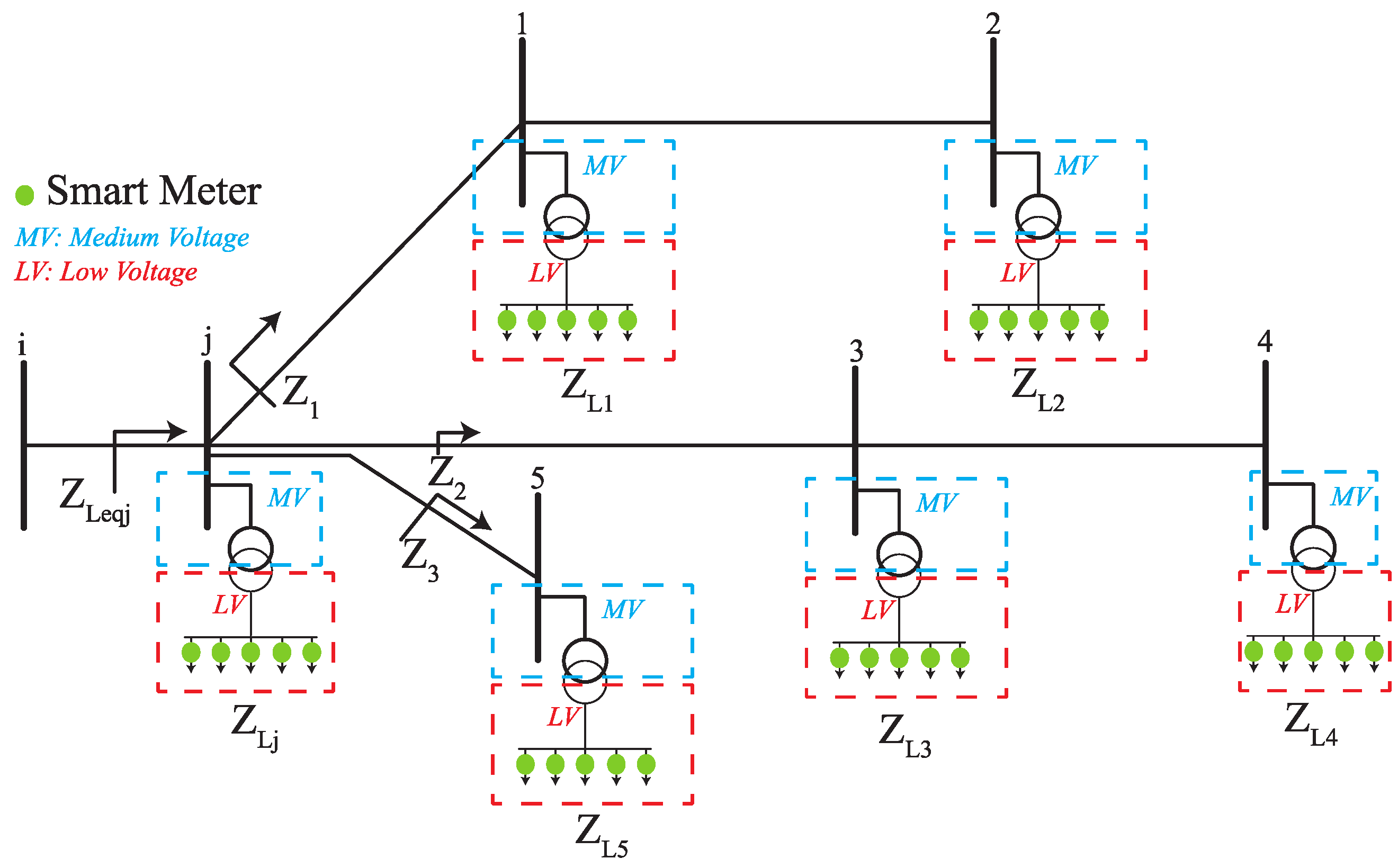
The impedance-based FL algorithm needs the value of each bus load. In the smart grids, SMs are located in the low voltage side of the network to periodically record the quantity of the network for the vast majority of applications, such as energy management, demand response, prediction application, load forecasting, and FL procedure. SMs can record the active and reactive power of each consumer, including industrial clients, and residential and commercial buildings. Based on the properties of SMs, these measurements could send the recorded quantities to the database center, with different time intervals. In this study, it is assumed that the active and reactive power of all nodes are available each minute. As an example of ELI calculation, a sample network depicted in Figure 1 is considered. In this figure, the SMs’ locations are considered on the low voltage side of the network. The recorded active and reactive power of all nodes and the recorded voltage and current at the beginning of the feeder is fed to a load flow method, to determine the voltage of all nodes. Therefore, the load impedance of node ( where is the number of network nodes) can be calculated using . The ELI at the end of section () is determined using each downstream node load impedance and DLPs. The DLPs model of a section is depicted in Figure 2. The ELI at the end of the section () is calculated by the following formula:
where is the ELI at the end of the section (). , , and are the upstream equivalent impedance of section (), section (), and section (), respectively. To determine these values, the DLPs model is utilized. The following equations are calculated to determine the upstream equivalent impedance of each section.
where and . Then using Equation (7), the ELI at the end of section () can be determined. The impedance-based FL method determines several answers as the location of the fault, but only one of these answers is the real fault point. In the next part, a new cost-effective method, which does not need any extra calculation, is presented to determine the real faulty section among all candidates, using SFM data.
2.3. Real Faulty Section Detection
As discussed earlier, the proposed impedance-based method uses periodically recorded active and reactive power of nodes and the phase-domain post-fault recorded voltage and current at the substation to locate a faulty section in the distribution network. Although, this method applies the minimum recorded information to locate the fault points that are more cost-effective and are faster, compared to intelligent, traveling wave, and differential equation-based methods, it determines several candidates as fault points. In fact, this happens because of only using the substation recorded data and the existence of many branches and sub-branches in distribution networks. Therefore, it is necessary to detect the real fault point among all acquired answers.
In this part, a new section estimation algorithm is presented, which uses the post-fault recorded information of SFMs. SFMs are measurement devices that locate on the medium voltage nodes. These devices measure phase-domain voltage, current, and active and reactive power of each node and the line connected to it. After a fault occurs in the network, the protection relays detect the fault in the network and send a fault pulse to all SFMs of the network to collecting the required information.
In the proposed faulty-section detection method, recorded post-fault active power of all located SFMs are utilized for detecting a real faulty section. In this method, it is not necessary to use SFMs on all nodes. To cost-effectively detect the real faulty section, SFMs locate on branches and sub-branches to fully support all sections of the network. For instance, in Figure 3, only three smart feeder meters are needed on nodes 2, 3, and 8 to determine the actual fault point. If a fault happens in section (2–6), due to the nature of the FL algorithm and the network topology, the algorithm may determine the section (2–6), (3–7), (3–4), (8–9), and (8–10), as well as the faulty sections. The substation relay sends a pulse to all SFMs for receiving the recorded post-fault active power. The recorded power of the real faulty section is much higher than the rest of the candidates due to the fault current. The flow-chart of the proposed algorithm is depicted in Figure 4. The proposed method steps are presented in Algorithm 1.
| Algorithm 1. Impedance-based FL algorithm | |
| Input—recorded data of voltage, current at the beginning of feeder, and the constant power of SFMs. | |
| 1: | Check if the fault is detected in the network or not |
| 2: | Determine the fault type (one or two) |
| 3: | The protection relay sends pulse to gather the recorded information of all SMs, SFMs, and substation measurement |
| 4: | Estimate the accurate load impedance of each node |
| 5: | if there are adequate SM then |
| 6: | Calculate the load impedance of each node using the recorded information of each SM at the low-voltage side of the network |
| 7: | else |
| 8: | Estimate the load value of each node using the method of [39] |
| 9: | end if |
| 10: | Calculate the equivalent impedance load at the end of each section |
| 11: | Determine post fault input voltage and current of each section |
| 12: | While there is a section for analyzing do |
| 13: | Calculate the fault current using (6) |
| 14: | Calculate the fault distance (1) or (2) |
| 15: | if the answer is not converged then |
| 16: | Calculate the fault point voltage using (3) |
| 17: | Update fault current using (4), (5), and (6) |
| 18: | Go to step 13 |
| 19: | else |
| 20: | Fault distance is determined |
| 21: | end if |
| 22: | Go to the next section |
| 23: | end while |
| 24: | if there is only one acceptable answer then |
| 25: | fault distance and faulty section are determined |
| 26: | else |
| 27: | Use the recorded active power of the branch related to the fault point |
| 28: | Set the section with the largest active power as a real faulty section |
| 29: | end if |
| 30: | Print the index of the actual faulty section and fault distance |
After a fault occurs in the network, the algorithm starts to locate the real faulty point. To determine the fault distance, Equation (1) is used for grounded faults and Equation (2) is used for phase-to-phase faults. The protection relays detect a fault in the network and send a signal to substation measurement and all smart measurement devices, such as SMs in the low-voltage side and SFMs in the medium-voltage side of the network, to collect the recorded pre- and post-fault data. The load value of each node should be determined for calculating the fault current and iterative computation. In this method, it is necessary to use the data of SMs in the low-voltage side of the network. However, in the case of lack of SMs in some nodes of the network, the load estimation method of [39] can be applied to accurately estimate the load value of each node. Equivalent load impedance at the end of each section should be specified as a result of analyzing all sections. Post-fault recorded information of the measurement located at the substation, distributed line parameters model, and Equations (1) and (2) are used to determine the fault distance of each node. Note that the determined fault distance must be a positive value and less than the analyzed section length. If the acquired answer was not acceptable, an iterative procedure should be performed using Equations (4)–(6). As there are many laterals and sub-laterals in the distribution network, there is a possibility of detecting several points as faulty sections. In this paper, the recorded active power of SFMs; which are located in the nodes with more than two connected lines; are used. The value of the active power is the indicator of the real faulty section. The section with the largest value of active power is the actual faulty section because of the high-fault current. In the next part, the simulation results are presented on the test feeder.
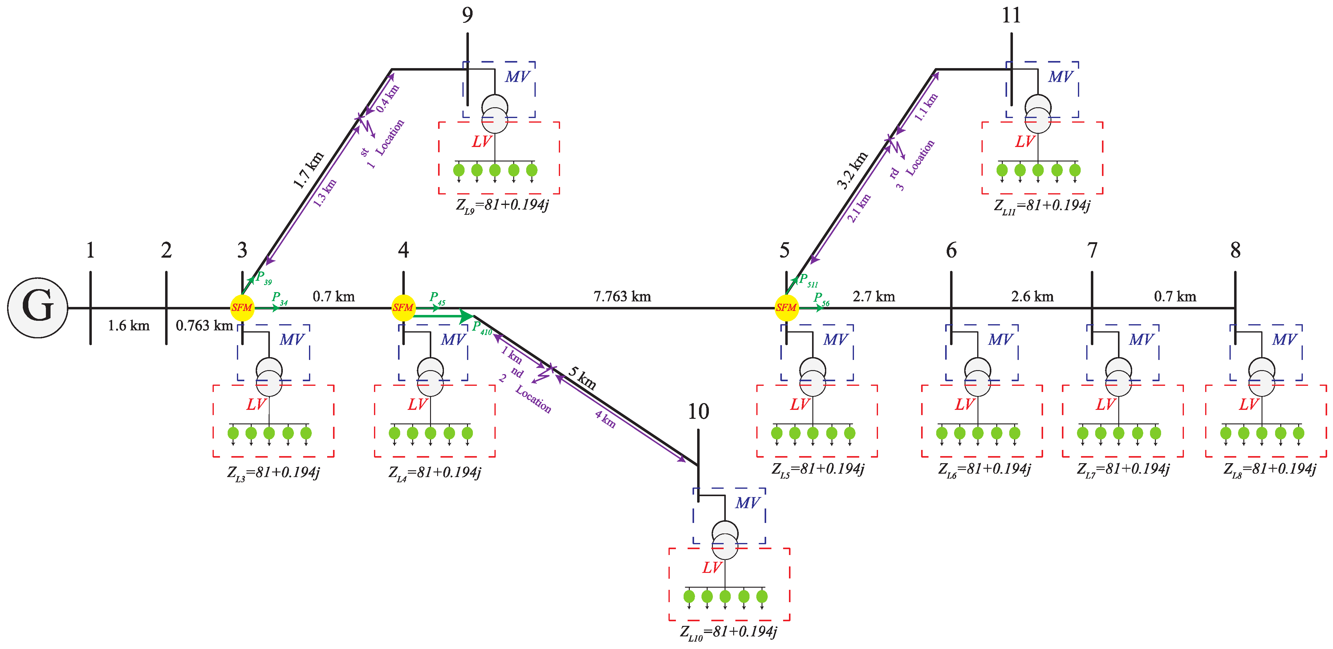
3. Simulation Results
To validate the effectiveness of the proposed method, several simulations were performed on the IEEE 11-node test feeder, as depicted in Figure 5 in SIMULINK MATLAB 2020b. There were 7 nodes in the main feeder of the network and nodes 9, 10, and 11 were connected to the main feeder to nodes 3, 4, and 5, respectively. These three branches were the main reason for the multiple solutions of the proposed FL algorithm. If a fault occurs in section (4–5), the proposed method may find three FL in sections (4–5), (3–9), and (4–5), based on the fault type and its distance on that section. Only one of these candidates is the actual point of fault. To overcome this difficulty, the proposed section estimation algorithm can differentiate between the real faulty section and other possible solutions. To this end, three SFMs are located in nodes 3, 4, and 5. The following fault conditions are considered to reveal the proposed method effectiveness:
- Different fault resistance (0-, 20-, 50-, 100-ohm).
- Different fault types (single-phase, two-phase and three-phase to ground).
- Different fault inception angles (0-, 30-, 70- and 150-degree).
- Different fault distances (sections (3–9), (4–10) and (5–11)).
- Laboratory single-phase fault experiment.
Distributed line model of each section was simulated to achieve a more precise result. After a fault occurs in the network, the recorded voltage and current at the beginning of the network and the last recorded power of SMs in the low voltage are fed to the load-flow algorithm, to achieve the voltage of each node and subsequently the impedance of each node. Using the phase-domain voltage, the current of the substation, the determined impedance value of each node, and the impedance-based FL algorithm, all possible locations of fault were calculated. Afterwards, the determined locations and recorded active power of SFMs regarding the FL candidates were applied to the section estimation method to distinguish the real fault point from the rest of the nominees. The following scenarios were investigated to reveal the proposed method effectiveness.
3.1. Different Fault Distances
Faults may unexpectedly occur in the distribution networks in any location of the network. This could happen in the main feeder or in the laterals or sub-laterals of the network. Therefore, the FL method should be able to perform well in the face of such difficulty. To examine the proposed method performance in different FLs, several simulations of three-phase to ground fault with 50-ohm ground resistance were performed in sections (3–9), (4–10), and (5–11) in the distance of 3.663 km, 4.063 km, and 12.926 km from the substation. The results of the simulations are presented in Table 1. For the first case, three candidates of FL was determined by the algorithm in the real sections (section (3–9), section (4–5), and section (4–10) in 3.6585 km, 3.6567 km, and 3.6571 km of the beginning of feeder, respectively). To exactly specify the location of the fault, the output active power of each upstream node of the candidate section is reported. The maximum value of active power represents the real section of the fault.
3.2. Different Fault Resistances
Impedance-based algorithms determine the location of faults in the networks by investigating the change in the impedance of each network’s section. Due to the vastness of electricity distribution networks, the need to supply energy to all consumers and the existence of different types of land in an area including asphalt, sand, stone, etc., the fault may occur with any resistance in the network. Hence, a FL method has to be robust against this problem. To this end, several simulations of single-phase to ground fault with 0-, 20-, 50-, and 100-ohm in section (3–9) (3.663 km from the substation) were carried out to demonstrate the proposed method’s effectiveness against various ground fault impedances. Based on the result of Table 2, the proposed method could differentiate between the real location of fault and nominees. For instance, three candidates were specified as FLs in sections (4–5), (3–9), and (4–10) for the 100-ohm ground fault case. The recorded active power of SFMs located in nodes 3, 4, and 5 revealed that the output power value for the real faulty section was much higher than other points. It can be seen from the results of Table 2 that the proposed section estimation method can easily detect the fault section among all candidates.
3.3. Different Fault Inception Angles
Fault happens in the network due to many reasons such as adverse weather conditions, falling external objects like a tree, and aging of the network’s equipment. Since all of these situations may arise in an unpredictable manner, the fault inception angle could randomly take place in a boundary of . This requires that the FL algorithm be able to operate correctly for all fault inception angles. Several different cases of the starting fault angle for a two-phase fault to ground with 50-ohm fault resistance were simulated, and the results are reported in Table 3. Four cases of fault angle with 0-, 30-, 70-, and 150-degree in section (4–10) (4.063 km from the substation) were considered. The results revealed that the section estimation algorithm could perfectly distinguish an actual fault point from other answers.
3.4. Different Fault Types
Several types of faults could occur in the network that could adversely affect the FL algorithms. Accordingly, in this paper, a powerful method is presented to determine the actual section of fault among all fault point candidates. Single-phase, two-phase, and three-phase to ground faults with different situations were simulated in the test feeder. The results of several single-phase faults with different ground fault resistances, two-phase faults with different fault starting angles, and three-phase faults in different spots of the network were simulated. The results are reported in Table 1, Table 2 and Table 3, which revealed that this method could specify the location of different faults, regardless of their type.
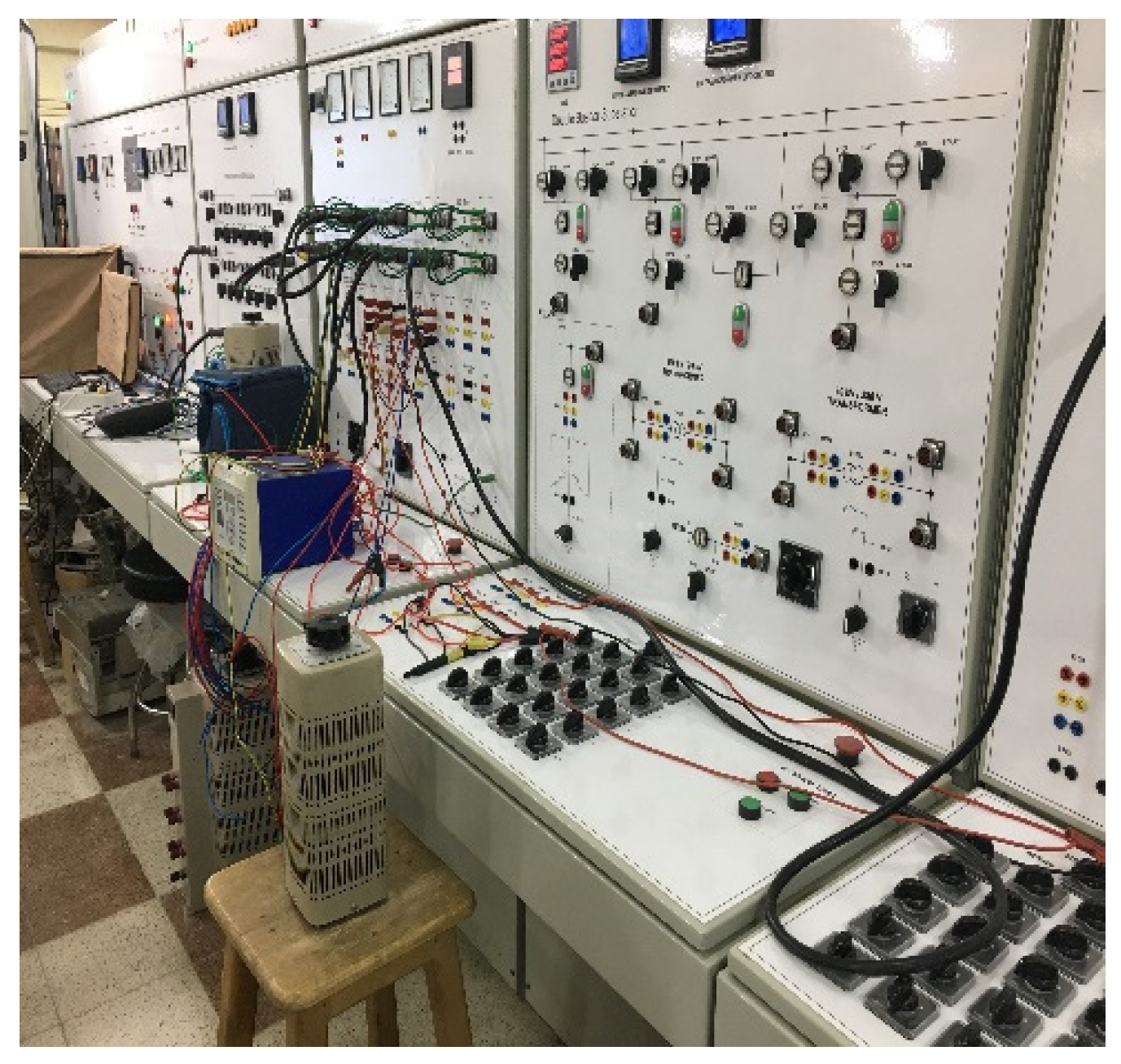
3.5. Laboratory Single Phase Experiment
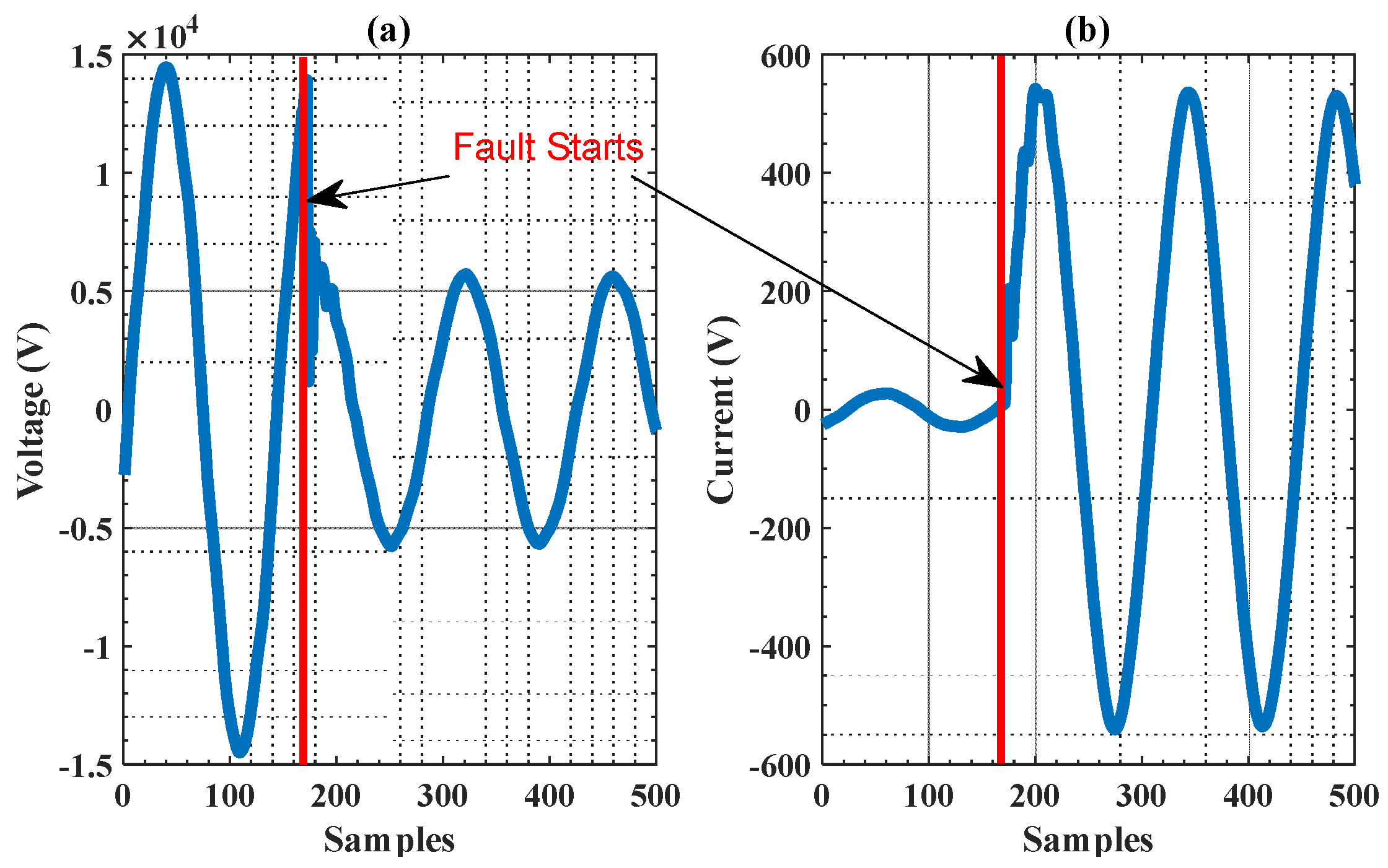
For further evaluation of the proposed method, its performance in a real test was examined. To this end, a solid single-phase fault experiment was performed on the power simulator set depicted in Figure 6. The waveforms of the recorded current, and voltage at the beginning of the feeder are demonstrated in Figure 7. A single-line view of the test network is shown in Figure 8. There were four nodes in the main feeder with two branches that consisted of four laterals. Three resistive loads were connected to nodes 4 (), 6 (), and 8 (). A fault occurred at a 15-km distance from node 3 in section (3–4). Three locations were determined in sections (3–6), (3–4), and (3–8) at , , and from the substation. The output power of each line from node 3 to nodes 6, 4, and 8 were recorded. These values were recorded by a power quality analyzer. Based on the recorded values, the real faulty section was section (3–4). The simulation with the same properties of the laboratory network was performed in MATLAB. The results of the simulation and laboratory test are presented in Table 4. As can be seen from the result, the proposed method was able to distinguish the real location of fault from other candidates.
4. Conclusions
Faults can cause outages and disruption and bring about financial losses, customer dissatisfaction, and reliability reduction, which is important for the distribution grid operators. In this paper, a new real FL, based on the variation of the impedance of the network is presented. This method could determine the real location of fault between all candidates that the FL algorithm may calculate. The recorded data of SMs in the low voltage and SFMs in the medium voltage is utilized and fed to the load-flow algorithm, for the next steps of the FL procedure. The recorded power of SFMs distinguished the real location of fault from other fault candidates. Several simulations were performed on the IEEE 11-node test feeder to investigate the proposed method’s effectiveness. The simulation results showed that the proposed section estimation method can easily identify the real faulty section in different fault conditions, such as different locations of fault, various types of fault, different fault inception angles, and single-, two-, and three-phase to ground faults. To practically examine the usefulness of FL, a single-phase laboratory test was carried out on the power simulator. The simulation of the laboratory test was also performed in MATLAB. In both simulation and laboratory tests of the sample network, the real faulty section was successfully determined. The results revealed that the proposed method is robust against different fault conditions, which occur unexpectedly.
Author Contributions
H.M.: Conceptualization, Data curation, Formal analysis, Investigation, Methodology, Validation, Writing—original draft. R.D.: Conceptualization, Funding acquisition, Investigation, Methodology, Project administration, Resources, Supervision, Writing—original draft. K.H.: Conceptualization, Funding acquisition, Project administration, Resources, Writing—review & editing. H.R.S.: Conceptualization, Funding acquisition, Project administration, Supervision, Writing—review & editing. All authors have read and agreed to the published version of the manuscript.
Funding
This work is supported by “Smart Fault Prediction and Location for Distribution Grids” project, funded by the Danish Energy Agency under the Energy Technology Development and Demonstration Program, ID number: 64019-0592.
Conflicts of Interest
The authors declare no conflict of interest.
References
- Celli, G.; Ghiani, E.; Pilo, F.; Soma, G.G. Reliability assessment in smart distribution networks. Electr. Power Syst. Res. 2013, 104, 164–175. [Google Scholar] [CrossRef]
- Mirshekali, H.; Dashti, R.; Shaker, H.R.; Samsami, R.; Torabi, A.J. Linear and Nonlinear Fault Location in Smart Distribution Network under Line Parameter Uncertainty. IEEE Trans. Ind. Inform. 2021. [Google Scholar] [CrossRef]
- Yu, K.; Zeng, J.; Zeng, X.; Xu, F.; Ye, Y.; Ni, Y. A Novel Traveling Wave Fault Location Method for Transmission Network Based on Directed Tree Model and Linear Fitting. IEEE Access 2020, 8, 122610–122625. [Google Scholar] [CrossRef]
- Yu, J.J.Q.; Hou, Y.; Lam, A.Y.S.; Li, V.O.K. Intelligent fault detection scheme for microgrids with wavelet-based deep neural networks. IEEE Trans. Smart Grid 2019, 10, 1694–1703. [Google Scholar] [CrossRef]
- Dehghanpour, K.; Wang, Z.; Wang, J.; Yuan, Y.; Bu, F. A survey on state estimation techniques and challenges in smart distribution systems. IEEE Trans. Smart Grid 2019, 10, 2312–2322. [Google Scholar] [CrossRef] [Green Version]
- Dashti, R.; Daisy, M.; Shaker, H.R.; Tahavori, M. Impedance-Based Fault Location Method for Four-Wire Power Distribution Networks. IEEE Access 2017, 6, 1342–1349. [Google Scholar] [CrossRef]
- Aftab, M.A.; Hussain, S.M.S.; Ali, I.; Ustun, T.S. Dynamic protection of power systems with high penetration of renewables: A review of the traveling wave based fault location techniques. Int. J. Electr. Power Energy Syst. 2020, 114, 105410. [Google Scholar] [CrossRef]
- Xie, L.; Luo, L.; Li, Y.; Zhang, Y.; Cao, Y. A Traveling Wave-Based Fault Location Method Employing VMD-TEO for Distribution Network. IEEE Trans. Power Deliv. 2020, 35, 1987–1998. [Google Scholar] [CrossRef]
- Shi, S.; Zhu, B.; Lei, A.; Dong, X. Fault location for radial distribution network via topology and reclosure-generating traveling waves. IEEE Trans. Smart Grid 2019, 10, 6404–6413. [Google Scholar] [CrossRef]
- Liang, R.; Yang, Z.; Peng, N.; Liu, C.; Zare, F. Asynchronous fault location in transmission lines considering accurate variation of the ground-mode traveling wave velocity. Energies 2017, 10, 1957. [Google Scholar] [CrossRef] [Green Version]
- Tashakkori, A.; Wolfs, P.J.; Islam, S.; Abu-Siada, A. Fault Location on Radial Distribution Networks via Distributed Synchronized Traveling Wave Detectors. IEEE Trans. Power Deliv. 2020, 35, 1553–1562. [Google Scholar] [CrossRef]
- Shi, Y.; Zheng, T.; Yang, C. Reflected Traveling Wave Based Single-Ended Fault Location in Distribution Networks. Energies 2020, 13, 3917. [Google Scholar] [CrossRef]
- Qiao, J.; Yin, X.; Wang, Y.; Xu, W.; Tan, L. A multi-terminal traveling wave fault location method for active distribution network based on residual clustering. Int. J. Electr. Power Energy Syst. 2021, 131, 107070. [Google Scholar] [CrossRef]
- Liang, R.; Wang, F.; Fu, G.; Xue, X.; Zhou, R. A general fault location method in complex power grid based on wide-area traveling wave data acquisition. Int. J. Electr. Power Energy Syst. 2016, 83, 213–218. [Google Scholar] [CrossRef]
- Jianwen, Z.; Hui, H.; Yu, G.; Yongping, H.; Shuping, G.; Jianan, L. Single-phase ground fault location method for distribution network based on traveling wave time-frequency characteristics. Electr. Power Syst. Res. 2020, 186, 106401. [Google Scholar] [CrossRef]
- Mamuya, Y.D.; Lee, Y.-D.; Shen, J.-W.; Shafiullah, M.; Kuo, C.-C. Application of Machine Learning for Fault Classification and Location in a Radial Distribution Grid. Appl. Sci. 2020, 10, 4965. [Google Scholar] [CrossRef]
- Shafiullah, M.; Abido, M.A.; Al-Hamouz, Z. Wavelet-based extreme learning machine for distribution grid fault location. IET Gener. Transm. Distrib. 2017, 11, 4256–4263. [Google Scholar] [CrossRef]
- Liang, J.; Jing, T.; Niu, H.; Wang, J. Two-Terminal Fault Location Method of Distribution Network Based on Adaptive Convolution Neural Network. IEEE Access 2020, 8, 54035–54043. [Google Scholar] [CrossRef]
- Dashtdar, M.; Dashtdar, M. Fault Location in Radial Distribution Network Based on Fault Current Profile and the Artificial Neural Network. Mapta J. Electr. Comput. Eng. 2020, 2, 30–41. [Google Scholar] [CrossRef]
- Shafiullah, M.; Abido, M.A.; Abdel-Fattah, T. Distribution grids fault location employing ST based optimized machine learning approach. Energies 2018, 11, 2328. [Google Scholar] [CrossRef] [Green Version]
- Deng, X.; Yuan, R.; Xiao, Z.; Li, T.; Wang, K.L.L. Fault location in loop distribution network using SVM technology. Int. J. Electr. Power Energy Syst. 2015, 65, 254–261. [Google Scholar] [CrossRef]
- Zhang, C.; Yuan, X.; Shi, M.; Yang, J.; Miao, H. Fault Location Method Based on SVM and Similarity Model Matching. Math. Probl. Eng. 2020, 2020, 2898479. [Google Scholar] [CrossRef]
- Akmaz, D.; Mamiş, M.S.; Arkan, M.; Tağluk, M.E. Transmission line fault location using traveling wave frequencies and extreme learning machine. Electr. Power Syst. Res. 2018, 155, 1–7. [Google Scholar] [CrossRef]
- Mirshekali, H.; Dashti, R.; Shaker, H.R. An Accurate Fault Location Algorithm for Smart Electrical Distribution Systems Equipped with Micro Phasor Mesaurement Units. In Proceedings of the 2019 International Symposium on Advanced Electrical and Communication Technologies (ISAECT), Rome, Italy, 27–29 November 2019; Institute of Electrical and Electronics Engineers Inc.: Interlaken, Switzerland, 2019. [Google Scholar] [CrossRef]
- Jamali, S.; Bahmanyar, A.; Bompard, E. Fault location method for distribution networks using smart meters. Meas. J. Int. Meas. Conf. 2017, 102, 150–157. [Google Scholar] [CrossRef]
- Gholami, M.; Abbaspour, A.; Moeini-Aghtaie, M.; Fotuhi-Firuzabad, M.; Lehtonen, M. Detecting the Location of Short-Circuit Faults in Active Distribution Network Using PMU-Based State Estimation. IEEE Trans. Smart Grid 2019, 11, 1396–1406. [Google Scholar] [CrossRef]
- Pignati, M.; Zanni, L.; Romano, P.; Cherkaoui, R.; Paolone, M. Fault Detection and Faulted Line Identification in Active Distribution Networks Using Synchrophasors-Based Real-Time State Estimation. IEEE Trans. Power Deliv. 2017, 32, 381–392. [Google Scholar] [CrossRef] [Green Version]
- Usman, M.U.; Omar Faruque, M. Validation of a PMU-based fault location identification method for smart distribution network with photovoltaics using real-time data. IET Gener. Transm. Distrib. 2018, 12, 5824–5833. [Google Scholar] [CrossRef]
- Jamali, S.; Bahmanyar, A. A new fault location method for distribution networks using sparse measurements. Int. J. Electr. Power Energy Syst. 2016, 81, 459–468. [Google Scholar] [CrossRef]
- Ghaedi, A.; Hamedani Golshan, M.E.; Sanaye-Pasand, M. Transmission line fault location based on three-phase state estimation framework considering measurement chain error model. Electr. Power Syst. Res. 2020, 178, 106048. [Google Scholar] [CrossRef]
- Langeroudi, A.T.; Abdelaziz, M.M.A. Preventative high impedance fault detection using distribution system state estimation. Electr. Power Syst. Res. 2020, 186, 106394. [Google Scholar] [CrossRef]
- Jia, K.; Bi, T.; Ren, Z.; Thomas, D.W.P.; Sumner, M. High frequency impedance based fault location in distribution system with DGs. IEEE Trans. Smart Grid 2018, 9, 807–816. [Google Scholar] [CrossRef]
- Gabr, M.A.; Ibrahim, D.K.; Ahmed, E.S.; Gilany, M.I. A new impedance-based fault location scheme for overhead unbalanced radial distribution networks. Electr. Power Syst. Res. 2017, 142, 153–162. [Google Scholar] [CrossRef]
- Orozco-Henao, C.; Bretas, A.S.; Marín-Quintero, J.; Herrera-Orozco, A.; Pulgarín-Rivera, J.D.; Velez, J.C. Adaptive impedance-based fault location algorithm for active distribution networks. Appl. Sci. 2018, 8, 1563. [Google Scholar] [CrossRef] [Green Version]
- Aboshady, F.M.; Thomas, D.W.P.; Sumner, M. A new single end wideband impedance based fault location scheme for distribution systems. Electr. Power Syst. Res. 2019, 173, 263–270. [Google Scholar] [CrossRef]
- Dashti, R.; Salehizadeh, S.M.; Shaker, H.R.; Tahavori, M. Fault location in double circuit medium power distribution networks using an impedance-based method. Appl. Sci. 2018, 8, 1034. [Google Scholar] [CrossRef] [Green Version]
- Dashti, R.; Sadeh, J. Accuracy improvement of impedance-based fault location method for power distribution network using distributed-parameter line model. Int. Trans. Electr. Energy Syst. 2014, 24, 318–334. [Google Scholar] [CrossRef]
- Dashti, R.; Sadeh, J. Fault section estimation in power distribution network using impedance-based fault distance calculation and frequency spectrum analysis. IET Gener. Transm. Distrib. 2014, 8, 1406–1417. [Google Scholar] [CrossRef]
- Mirshekali, H.; Dashti, R.; Keshavarz, A.; Torabi, A.J.; Shaker, H.R. A Novel Fault Location Methodology for Smart Distribution Networks. IEEE Trans. Smart Grid 2020, 12, 1277–1288. [Google Scholar] [CrossRef]
Figure 1.
Single line diagram of a sample network with SMs in the low voltage side of the network.

Figure 2.
Distributed line parameter model of each network’s section.

Figure 3.
A sample network equipped with SFMs located in nodes 2, 3, and 8.

Figure 4.
Flow-chart of the proposed method.

Figure 5.
Single line diagram of IEEE 11-node test feeder equipped with smart meters and SFMs.

Figure 6.
Power simulator set.

Figure 7.
Recorded voltage (a) and current (b) waveforms.

Figure 8.
Single line diagram of the laboratory test network.


Table 1.
Proposed Method Effectiveness under Different Fault Locations.
| Fault Locations | First Candidate | Second Candidate | Third Candidate |
|---|---|---|---|
| Section (3–9) 3.663 km | Section (4–5) 3.6567 km | Section (3–9) 3.6585 km | Section (4–10) 3.6571 km |
| Section (4–10) 4.063 km | Section (3–9) 3.3547 km | Section (4–5) 4.7575 km | Section (4–10) 4.0555 km |
| Section (5–11) 12.926 km | Section (5–11) 12.8973 km | Section (4–10) 5.1364 km | - |
Table 2.
Proposed Method Effectiveness under Different Fault Resistances.
| Fault Resistances | First Candidate | Second Candidate | Third Candidate |
|---|---|---|---|
| 0 | Section (4–5) 3.6373 km | Section (3–9) 3.6126 km | Section (4–10) 3.6271 km |
| 20 | Section (4–5) 3.543 km | Section (3–9) 3.6629 km | Section (4–10) 3.5792 km |
| 50 | Section (4–5) 3.3776 km | Section (3–9) 3.6649 km | Section (4–10) 3.4424 km |
| 100 | Section (4–5) 3.1899 km | Section (3–9) 3.6722 km | Section (4–10) 3.2388 km |
Table 3.
Proposed Method Effectiveness under Different Fault Inception Angles.
| Fault Resistances | First Candidate | Second Candidate | Third Candidate |
|---|---|---|---|
| 0 | Section (4–5) 3.9419 km | Section (3–9) 3.9463 km | Section (4–10) 3.9434 km |
| 30 | Section (4–5) 4.0021 km | Section (3–9) 4.0066 km | Section (4–10) 4.0037 km |
| 70 | Section (4–5) 4.1302 km | --- | Section (4–10) 4.1319 km |
| 150 | Section (4–5) 4.3144 km | --- | Section (4–10) 4.3161 km |
Table 4.
Laboratory and simulation result of single-phase to ground fault.
| Test Type | First Candidate | Second Candidate | Third Candidate |
|---|---|---|---|
| Simulation | Section (3–6) 101.4 km | Section (3–8) 101.1 km | Section (3–4) 100.96 km |
| Laboratory | Section (3–6) 105.56 km | Section (3–8) 106 km | Section (3–4) 104.2 km |
Publisher’s Note: MDPI stays neutral with regard to jurisdictional claims in published maps and institutional affiliations. |
© 2021 by the authors. Licensee MDPI, Basel, Switzerland. This article is an open access article distributed under the terms and conditions of the Creative Commons Attribution (CC BY) license (https://creativecommons.org/licenses/by/4.0/).
Share and Cite
MDPI and ACS Style
Mirshekali, H.; Dashti, R.; Handrup, K.; Shaker, H.R. Real Fault Location in a Distribution Network Using Smart Feeder Meter Data. Energies 2021, 14, 3242. https://doi.org/10.3390/en14113242
AMA Style
Mirshekali H, Dashti R, Handrup K, Shaker HR. Real Fault Location in a Distribution Network Using Smart Feeder Meter Data. Energies. 2021; 14(11):3242. https://doi.org/10.3390/en14113242
Chicago/Turabian StyleMirshekali, Hamid, Rahman Dashti, Karsten Handrup, and Hamid Reza Shaker. 2021. "Real Fault Location in a Distribution Network Using Smart Feeder Meter Data" Energies 14, no. 11: 3242. https://doi.org/10.3390/en14113242
Note that from the first issue of 2016, this journal uses article numbers instead of page numbers. See further details here.