Electricity Portfolio Optimization for Large Consumers: Iberian Electricity Market Case Study

Abstract

Electricity markets are nowadays flooded with uncertainties that rise from renewable energy applications, technological development, and fossil fuel prices fluctuation, among others. These aspects result in a lumpy electricity prices for consumers, making it necessary to come up with risk management tools to help them hedge this associated risk. In this work a portfolio optimization applied to electricity sector, is proposed. A mixed integer programming model is presented to characterize the electricity portfolio of large consumers. The energy sources available for the portfolio characterization are the day-ahead spot market, forward contracts, and self-generation. The study novelty highlights the energy portfolio characterization for players denoted as large consumers, which has been overlooked by the scientific community and, focuses on the Iberian electricity market as a real case study. A multi-objective methodology is explored, using a weighted-sum approach. The expected cost and the conditional value-at-risk (CVaR) minimization are used as objective function. Three case studies illustrate the model applicability through the characterization of how the portfolio evolves with different demand profiles and how to take advantage from seasonality characteristic in the spot market. A scenario analysis is explored to reflect the uncertainty on the price of the spot market. The expected cost and CVaR are optimized for each case study and the portfolio analysis for each risk posture is characterized. The results illustrate the advantage to reduce costs and risk if the prices seasonality is considered, triggering to an adaptive seasonal behavior, which support the decision-maker decision towards its goals.

1. Introduction

One of the main issues for any industry is to fulfill its energy needs in the smartest way possible. However, the management of an energy portfolio should simultaneously: reduce the cost, manage the risk associated and satisfy the demand, increasing the management complexity. These aspects are often a concern in the literature given the many opportunities, the different methods and tools that can be used.

In addition, the energy sector is characterized by many risks, opportunities, given the technology and renewable energy developments, which allow the energy portfolio manager to take advantage of. Hence, one of today’s challenge is to use the energy resources available efficiently and towards to improvement of performance indicators as: cost, risk and renewable energy.

In the electricity sector we have three key players: the private investors, the managers commercializing energy and the planners. They all interact in the markets but face different problems and uncertainties, changing its behavior based on its preferences over tools or mechanisms of the markets [1]. The investors invest in technology mixes that favor them and maximize their profit, while planners seek social welfare maximization. The managers commercialize energy and their biggest concern is to maximize return and minimize risk. The latter includes both the buyers and sellers of energy [2]. Although the managers’ side is nowadays key in electricity markets, their risk management problems are less developed than the planners’ [1]. These players resort to electricity markets to contract their energy needs, with few available tools that can use and take advantage of, to develop a long-term and short-term plan.

Electricity markets worldwide normally offer two types of market structure to trade energy: spot (or day-ahead or pool) market and forward market. The spot market is the energy traded in the real time and day-ahead market and the most popular structure is a centralized pool-base auction where the buyers and sellers submit bids [3]. The corresponding problem, with a different approach, was considered for the electricity balance market with the use of a historical data set and the best-known solutions have been improved [4]. However, drawback spot market is its price volatility, being the highest when compared to any other commodities’ spot markets [5]. Although, the forward markets is seen as the way, to overcome the lumpy prices in the spot market, where with forward contracts, consumers and suppliers commit on the trading of a specific amount of electricity, at a specific future time against a fixed price [6]. There are several European electricity markets where the players can interact. As example, there is the Iberian electricity market, which is operated by OMIE, which is the nominated electricity market operator, responsible for managing the Iberian Peninsula’s day-ahead and intraday electricity markets [7].

These electricity markets are nowadays flooded by numerous sources of uncertainty that arise since the sector itself and historically, are particularly unpredictable. Hence, to plan over it, is necessary to predict which future conditions the market may face, such as: how will the fossil fuel prices evolve, what will be the demand profile, will the electricity generation still so hardly depend on fossil fuels. The literature over the last two decades has primarily focused on the uncertainties that come from such factors as fuel prices, demand growth and CO2 prices. However, other factors, such as renewable resources availability, technology development, social opposition and emissions limits, also play an important role [2].

In some cases, a linear programming formulation can be proposed to characterize, not only, the distribution network characteristics, but also, consider the market compensation processes for flexible charging and distributed energy resources, leading to reserve and reactive power compensation [8].

Given all the opportunities and threads present in the energy sector, it is important for any consumer to best take advantage in the procurement of its energy needs. To do so, a proper portfolio optimization would be essential. However, regarding electricity markets, literature has paid little attention to the buyer’s perspective and so, the goal of this article is to make a contribution in this direction. To do so, a portfolio optimization for a large consumer is conducted, with the aim of simultaneously reducing the expected cost and minimizing the risk associated. A mixed integer linear formulation is proposed to support the decision-maker, while the trade-off between several optimal alternatives are provided, leading to energy portfolio characterization. The problem addressed is an energy portfolio optimization for a large consumer, using a multi-objective approach to minimize the total expected cost and risk associated.

The study has the following structure: in Section 1, an introduction is made, where the background and general motivation are set, the characterization of the electricity markets is provided, as well as the objectives and article structure. In Section 2 explores the literature review focus in methods and trend of energy transition from a circular economy perspective. In Section 3 is defined the methodology to be used: steps of the analysis and problem characterization. The mathematical formulation is presented in Section 4, followed by the explanation of how the data were collected and how was it was fitted, in Section 5. In Section 6 is shown the results and its analysis from three case studies. Finally, general conclusions and further work are considered on Section 7.

2. Literature Review

2.1. Energy Transitions from a Circular Economy Perspective

At this moment, the trend is the energy transition to renewable energy sources, with the aim of, not only, reducing consumption of fossil fuel, but also, to switch parts in the electricity systems, within a circular economy perspective. Therefore, some research was done by several authors exploring these subjects, mainly:

The paper [9] discussed the potential energy future perspectives and proposed a topology. As a result, the authors conclude, that potential energy futures, not only are a simple function of the technologies employed and their scale, but also, they will be shaped by the social relations that configure societies in general.

Authors in [10] examined the impacts of biowaste-based energy transition, through a semi-quantitative evaluation by engaging the relevant social stakeholders’ evaluation in the strategic plan. The proposed decision-making tool uses analytics and optimization algorithms to guide competent authorities and decision-makers to sustainable energy transitioning towards decarbonization.

Work [11] provided the most effective instrument mix for energy transition in biofuel industry based on the case of the Italian liquid biofuel sector. The simulations results showed the persistence of negative context conditions would be detrimental for the convergence of expectations, providing clear priorities in setting the energy policy agenda.

Research [12] introduced the green finance gap for the transition to a low carbon economy. Considering the government policy to finance early stage green innovations.

Finally, paper [13] discussed energy and bio-products production based on resource circularity in the tourism industry. Research has shed light on external pressures and internal dynamics to provide a clear direction for policy strategies to support the transition towards a tourism-based circular economy. An integrated SWOT-MLP framework has been built to provide crucial theoretical perceptions for the transition under investigation.

2.2. Multi-Objective Optimization

Multi-objective optimization (MOO) is a growing subject in the engineering world today given the conflicting nature of the multiple objectives of today’s real-world problems. Although the ideal would be to optimize all the objectives simultaneously, that is very complex due to their high number and the competition between them. Based on this, the optimization approaches have to make compromise and deliver several solutions [14,15].

The usual process in multi-criteria optimization is to find all non-dominated or Pareto optimal solutions of the problem, for instance, every solution, which we cannot improve with one objective function without deteriorating another [16,17].

There are multiple techniques to solve MOO problems, such as: weighted sum method, ε-constraint, lexicographic approach, reference points or sets methods, goal programming, etc. The weighted sum approach gives weights to each objective function and transforms it into a single objective. The ε-constraint method, proposed by [18], selects one objective to be minimized/maximized and constrains the remaining objectives functions to be less or equal to a target value. Goal programming does not pose the question of maximizing multiple objectives, but it rather sets specific goals for each objective and attempts to find them [19]. Most of the traditional algorithms tackle the MOO problem by transforming it into a single-objective function with the weighted-sum method [20]. Examples of this application are found in [21,22].

2.3. Portfolio Optimization with Downside Risk: Conditional Value-at-Risk

The modern portfolio theory era was first started by [23] and, since then become the most common way for investors to deal with expected returns, costs and uncertainty for a large number of problems. The portfolio optimization problem was first formulated looking at the expected return and risk, with focus in the expected return variability, which found a high popularity in finance sector. The nature of the multi-objective portfolio problems was presented in [16], with mixed integer linear programming multi-objective portfolio optimization approaches were discussed. Portfolio optimization has found popularity in the energy sector since it exploits the diversification idea through the “cancellation effect” [1].

Among the several techniques proposed to tackle the problem of portfolio selection, the risk measures became relevant and the downside risk is one of them [24]. As shown in works of [24,25], the portfolio formulation has enabled the two most popular financial engineering percentile risk measures, value-at-risk (VaR) and conditional value-at-risk (CVaR) to be used. Downside risk reflects the negative deviations from the expected return, focusing on the side that takes loss, opposite to the mean variance [23], that assesses in the same way upside and downside risks [26]. Initially introduced by [27], the CVaR deals with the “conditional expectation of losses in the top 100 × (1-α)%” assuming a specific level of α. The CVaR denotes the average of worst-cases loss scenarios for a specific level. While the VaR defines the “threshold level for losses in the top 100 × (1-α)%” [28] for a specific level of α. Common values considered for α are 0.90, 0.95 and 0.99 [29]. CVaR’s popularity has grown significantly in the literature [30,31,32,33] mostly due to VaR’s undesirable properties [34]. The author of [30] solved the portfolio optimization problem using a multi-objective approach and the VaR measure. The work [31] considers three different bi-objective formulations to explore the portfolio problem. First formulation considers the use of percentile risk measure, VaR, through a mixed integer linear programming. The second formulation considers the measure, CVaR using linear programming. The last one explores symmetric measure of risk, like in Markowitz [23] portfolio.

2.4. Energy and Electricity Portfolios

As previously stated, modern portfolio theory has seen its popularity growing in the energy sector in the last years, mostly on the planner’s side, standing as a widely accepted methodology to solve the long-term investment decisions in energy planning.

The planners´ considered in the literature review can be buyers or sellers in a liberalized market, as defined by [1,2]. These stakeholders need to allocate their electricity among different instruments, such as the day-ahead, real time markets and bilateral forward contracts. Hence, these agents can take advantage of portfolio optimization by diversifying throughout these instruments, as well as by choosing among generation technologies [34].

As examples of portfolio theory applications to the buyer’s perspective, there is the works of [6] and of [35]. Recently [36] examines a fuzzy multi-objective decision making structure established for optimization of renewable energy project portfolios. The energy portfolios were constructed [37] and three problems were analyzed. The first problem minimizes the worst cases volatility, with a certain fixed maximum expected energy costs [37]. The second minimize the worst cases expected costs, with certain fixed maximum of volatility for the energy costs [37]. While the third problem combine the expected and volatility of the costs and is weighted by a risk aversion parameter [37]. These portfolio models are formulated as quadratic, second order cone programming and semi definite programming, so that robust optimization tools have be implemented.

In work [38] the portfolio optimization is developed for an optimal scheduling strategy in a microgrid take part in an unstable electricity market. The modern portfolio theory [39] is enabled to define the efficient frontier of optimal variable renewable energy portfolios that summarize the geographical smoothing effect for future power system. Article [40] considers power portfolio optimization in a medium term, for a power producer in a competitive electricity market, considering electricity prices and risk management. The methodology developed considers the multivariate stochastic evolution of electricity prices and, the construction of a scenario tree to represent its evolution. Work [41] presents a portfolio optimization composed by end-use consumers, through the Markowitz Theory. An overview of a multi-agent system for electricity markets is also presented. Authors [42] propose two modern portfolio theory models. The first considers the Mean Variance Criterion and the second explores the CVaR. The electricity portfolio models are combined with a generalized autoregressive conditional heteroskedastic prediction technique to optimally diversify their energy portfolio.

In work [43] authors present a comprehensive study of mean-variance, downside and semi-variance methods for portfolio optimization in electricity markets and the corresponding approaches for maximization of the return, while risk is minimized. Optimization of the electricity markets under modern portfolio theory has a crucial role for financial decision-makers [43]. Power suppliers in deregulated electricity markets need to optimize their generation capacities and bidding strategies to effectively play a part in bilateral contract and spot markets. Market players must deal with continuously changes of electricity prices, in the competitive electricity market environment during their daily routine [43]. Despite electricity cannot be stored it can be generated and consumed simultaneously.

Authors [44] are focuses on more sustainable aspects, like the impact of renewable portfolio standards and emissions trading on the electricity market.

Work [45] presents a review and extend the stochastic Levelized Cost of Electricity (LCOE) portfolio theory and, the mean-risk analysis of electricity generation investment portfolios, taking into account the relation between risk and deviation risk measures in the purpose of shaping the risk distribution.

2.5. Scenario Analysis

Scenarios have become a fundamental part of foresight science and scenario planning is recognized as the most widely used method in the futures field.

Again, since the planner’s side is generally more developed, most of scenario analysis application are done on the planner’s perspective, which [46,47] are examples of.

From the buyer’s perspective we have the works of [48], that built a scenario tree as a tool to reflect the uncertainty shown in the price of the spot market.

2.6. Literature Review Summary

Overall conclusions are taken from the literature review:

• Bi-objective optimization is popular among the portfolio analysis given its easiness to present and conduct to the results; as a MOO method weighted sum is the most popular and consensual.
• As a risk measure for energy portfolio, mean-variance was preferred through time, however the more recent literature starts applying conditional value-at-risk and value-at-risk.
• The literature in electricity portfolios focuses mainly of the planner’s problems and challenges and there is a lack of work from the buyer perspective.

3. Methodology and Problem Statement

3.1. Methodology

The methodology undertaken in this work follows several steps and explores several methodologies. The first step identifies, in the literature review, the gap that remains to be fulfilled, considering the energy portfolio optimization of large consumer, from buyers’ perspective. Followed by the stakeholder’s identification and its roll characterization, mainly electricity suppliers’ options and large consumer needs. The Iberian Market is explored, as large consumer stakeholder. Three electricity suppliers’ options are considered: day-ahead market, forward contract and self-generation.

The forward contract will be set in a specific time and its output will be divided in 4 blocks of energy, each with a specific price. The self-generation energy implies a long-term investment, providing a constant energy throughout every hour of the planning horizon. A long-term investment aversion from the decision-maker must be considered. Its energy is divided in 4 blocks, each with a different price as well. The day-ahead market trading stands as the factor that brings uncertainty into the decision-making.

Data collecting and screening for further analysis and data characterization is performed. 48 weeks is considered as a final sample. However, this step is of high importance to grab the sector characteristics and feed the model with accurate information. Based on that, a deeper analysis over seasonality patterns identification is undertaken, such as: yearly, weekly and daily. Data categorization is undertaken according to their average spot price, in three categories: valley, shoulder and peak hours. Some parameters are estimated, and some information is omitted due confidentiality reasons.

The aim of this work is to explore the energy portfolio optimization considering simultaneously the cost and the risk, which trigger to a multi-objective approach. The trade-off between the two objectives is explored through the weighed-sum approach and its results characterized using the Pareto Font representation. An economic indicator, as costs is used as one of the objective functions, while a risk measure, as CVaR is explored to mitigate the risk.

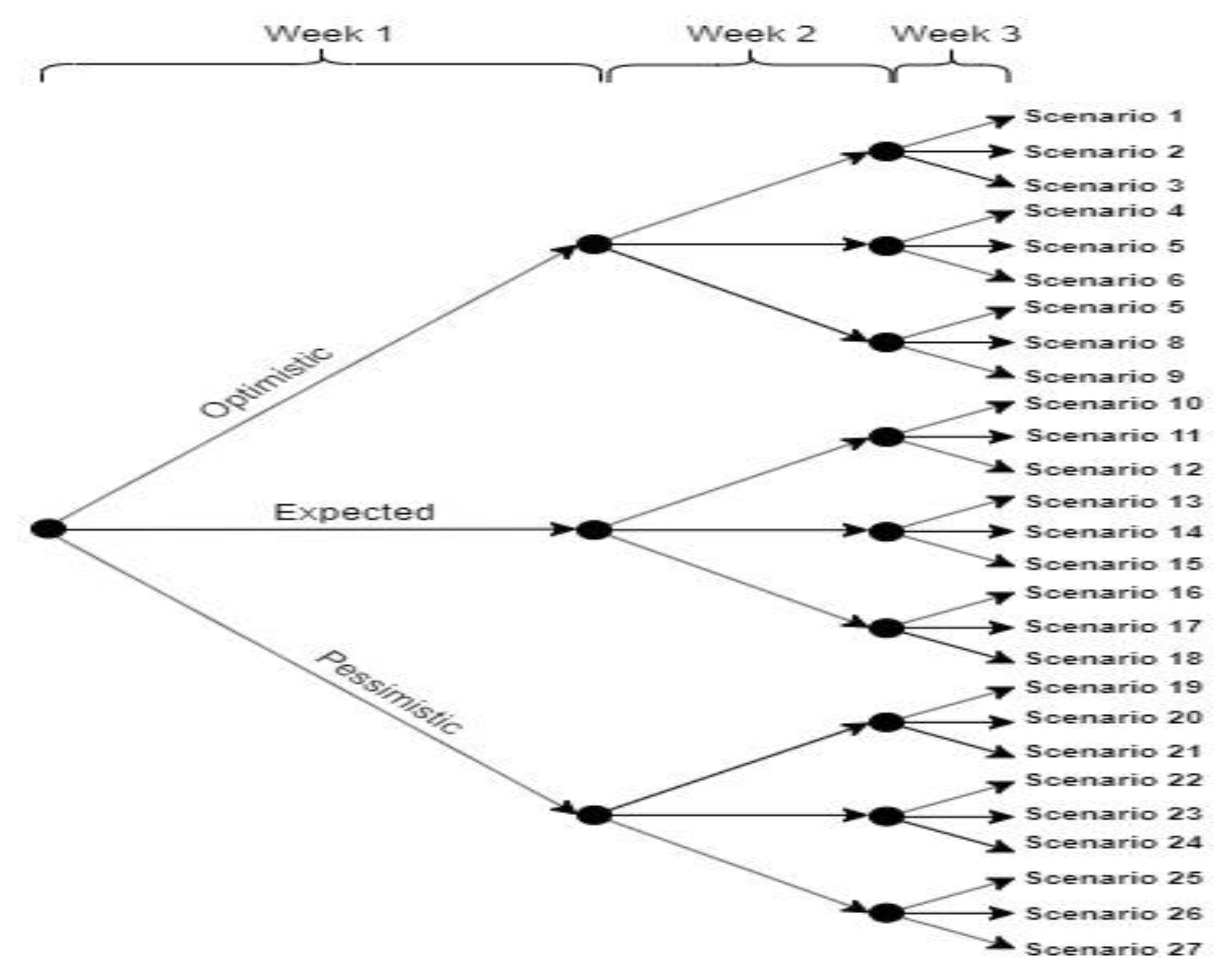
Another relevant aspect is the electricity market variability/uncertainty. Its behavior is characterized through a Scenario Tree approach [49], as defined in Figure 1. The scenario tree has 3 branches leaving each node and 3 nodes, resulting in 3³ = 27 scenarios. Each branch denotes one week, with a total planning horizon of 3 weeks. On each node decisions regarding weekly forward contracts and spot market trading are done and exclusively on the first node, the decisions regarding 3-week Contract and self-generation production are taken.

3.2. Problem Statement

A portfolio optimization for a large consumer is conducted, from a buyer´s perspective, mitigating expected cost and risk. The mixed integer linear programming formulation is extended from [40,48] and Iberian electricity market is used as large consumer.

Three different electricity supply options are considered: forward contracts, self-generation facilities and pool market trading. In the forward contracts a specific quantity of energy is purchase in advance, for a specific price, to be delivered in a specific time. The pool market trades in the day-ahead market. While the self-generation the decision-maker must embrace an investment to pursue this option.

Hence, given sources price, scenarios and its probability, demand to be satisfied, the aversion to long term investment from the decision-maker and the confidence level for the CVaR calculation.

The model determines: procurement of electricity on each of the electricity options, the optimized scheduled and the non-dominate solution, allowing the trade-off between the expected cost and the CVaR, for several risk postures.

It is subject to: expected cost and CVaR minimization.

4. Mathematical Formulation

This work is extended from [48], with the aim of support the large consumer, from a buyer perspective, in the electricity portfolio optimization. A mixed integer linear program (MILP) based on [48] is proposed to simultaneously minimize the cost and risk.

4.1. Forward Contract

Notation:
Index
s	= Week
d	= Day
t	= Hour
w	= Scenario
c	= Contract
b	= Block
g	= Self-generation facility
k	= Stage
Sets:
Ns	= {s: set of weeks in the planning horizon}
Nd	= {d: set of days in the planning horizon}
Nt	= {t: set of hours in a day}
Nw	= {w: set of scenarios}
Nc	= {c: set of contracts available}
Nb	= {b: set of blocks available in each forward contract}
Ng	= {g: set of generation facilities}
Nk	= {k: set of stages}
CDs	= {c: set of forward contracts available in week s}
CTt	= {c: set of forward contracts available at hour t}
Data Parameters:
H	= Number of hours in the planning horizon
$E_{c,b}^{C_{\max }}$	= Maximum amount of energy available for contract c in block b (MWh)
$E_{c,b}^{C_{\min }}$	= Minimum amount of energy to be consumed from contract c in block b (MWh)
$P_{c,b}^C$	= Price of energy unit of contract c for block b (€/MWh)
$E_{g,b}^{G\min }$	= Minimum energy to be generated from self-generation facility g in block b (MWh)
$E_{g,b}^{G\max }$	= Maximum energy to be generated from self-generation facility g in block b (MWh)
$P_{g,b}^G$	= Levelized cost of energy unit from self-generation facility g (€/MWh)
$D_d^t$	= Demand of energy for day d at t (MWh)
${\pi }_w$	= Probability of scenario w
A	= Non-anticipativity matrix.
$K_c$	= Stage at which a decision for forward contract c is made
Parameters defined by the Decision-maker:
$\beta$	= Risk aversion factor
$\lambda$	= Aversion factor to long-term generation investment
$\alpha$	= Confidence level
Binary Variables:
$S_{c,w}^C$	= 1 if forward contract c is selected in scenario w, 0 otherwise
$S_g^G$	= 1 if self-generation investment g is selected, 0 otherwise
Variables:
$E_{c,b,w}^C$	= Amount of energy contracted from contract c and block b for scenario w (MWh)
$E_{g,b}^G$	= Amount of energy self-generated from g in block b (MWh)
$E_{s,d,t,w}^P$	= Amount of energy purchased from the pool for week s, day d and hour t in scenario w (MWh)
$C_w^C$	= Forward costs contracting (€)
$C_g$	= Total levelized cost of self-generation for the whole planning horizon (€)
$C_w^P$	= Purchases cost for the pool (€)
CVaR	= Conditional value-at-risk
$\xi$	= Value at risk
${\eta }_w$	= Auxiliary variable for CVaR
OF	= Objective function

The forward contracts use weekly intervals and deliver the same quantity of energy each hour over the contract horizon and can be set on single or multiple week’s bases. The energy available in each contract, c, for a block, b, must verify its capacity, Equation (1).

$$E_{c,b}^{C_{\min }}\times s_{c,w}^C\le E_{c,b,w}^C\le E_{c,b}^{C_{\max }}\times s_{c,w}^C\forall c\in N_c,\forall b\in N_b,\forall w\in N_w$$

(1)

The $E_{c,b,w}^C$ quantify the amount of energy contracted in contract c, for block b, in scenario w. The binary variable $s_{c,w}^C$ is equal to 1, if contract c is assigned in scenario w, 0 otherwise. The parameters $E_{c,b}^{Cmax}$ and $E_{c,b}^{Cmin}$ define the maximum and minimum amounts of electricity, respectively.

Its cost is quantified in variable $C_w^C$ in Equation (2). The parameter ${\mathrm{P}}_{\mathrm{c},\mathrm{b}}^{\mathrm{C}}$ defines the price for the block b, in contract c, which is available in week s, ${\mathrm{CD}}_{\mathrm{s}}$ and, at hour t ${\mathrm{CT}}_{\mathrm{t}}$.

$$C_w^C=7\times {\displaystyle \sum _s^{N_s}{\displaystyle \sum _t^{N_t}({\displaystyle \sum _{c\in (C{D}_s\cap C{T}_t)}{\displaystyle \sum _b^{N_b}}}}}{E}_{c,b,w}^C\times P_{c,b}^C)\forall w\in N_w$$

(2)

In forward contracts, the dependency between different scenarios regarding contract decisions is guaranteed through non-anticipativity constraints. Scenarios that are equal until a certain decision stage, should have the same decisions made until that stage, which is guaranteed by Equation (3). As done in [34], using a matrix of 0 s and 1 s where A(w, k) is equal to 1 scenario w and w+1 are equal up to stage k, 0 otherwise. Hence, the matrix’s size is (N_w − 1) × (N_k − 1), which in our case is a 26 × 3 matrix. Using A we can formulate the constraint as done in (3). The ${\mathrm{K}}_{\mathrm{c}}$ defines the stage at which a decision on contract, c is undertaken.

$$E_{c,b,w}^C=E_{c,b,w+1}^C\forall c\in N_c,\forall b\in N_b,\forall w\in N_w-1$$

(3)

4.2. Self-Generation Facilities

Self-generation facilities are a source of electricity, which must satisfy the minimum and maximum self-generation capacities, as in Equation (4).

$$E_{g,b}^{G_{\min }}\times s_g^G\le E_{g,b}^G\le E_{g,b}^{G_{\max }}\times s_g^G\forall g\in N_g,\forall b\in N_b$$

(4)

The $E_{g,b}^G$ quantifies the amount of energy self-generated in the facility g. The binary variable $s_g^G$ takes the value 1, if the self-generated facility g is installed, 0 otherwise. The $E_{g,b}^{Gmax },E_{g,b}^{Gmin}$ defines, respectively, the maximum and the minimum energy self-generated,

The cost of the self-generation facilities is given by Equation (5), with the H as the planning horizon and, $P_{g,b}^G$ the price per energy unit.

$$C^g={\displaystyle \sum _g^{N_g}H}\times {\displaystyle \sum _b^{N_b}{P}_{g,b}^G\times E_{g,b}^G}$$

(5)

4.3. Day-Ahead Spot Market and Energy Balance

In the day-ahead spot market is assumed that the costumer is a price-taker and, by that, its trades don´t impact in the market-clearing price. There is no real need to constrain the trade in the spot market. However, is necessary to guarantee the consumer only interacts as a buyer and guarantee that the self-generated electricity is not sold (partial self-generation are not allowed). Must be guranted that the energy procured from the day-ahead market, $E_{s,d,t,w}^P$, must be positive by Equation (6).

$$0\le E_{s,d,t,w}^P\forall d\in N_d,\forall t\in N_t,\forall w\in N_w,\forall s\in N_s$$

(6)

The cost is defined by Equation (7), the parameter, ${\mathrm{P}}_{\mathrm{s},\mathrm{d},\mathrm{t},\mathrm{w}}^{\mathrm{P}}$, quantify the price, per energy unit.

$$C_w^P={\displaystyle \sum _s^{N_s}{\displaystyle \sum _t^{N_t}{\displaystyle \sum _d^{N_d}{E}_{s,d,t,w}^P\times P_{s,d,t,w}^P}}}\forall w\in N_w$$

(7)

The energy balance constraint, Equation (8), ensures the energy available per hour, from the three different sources: self-generated, forward contracted and the spot market, must satisfy the demand $D_{d,t}$.

$${\displaystyle \sum _g^{N_g}{\displaystyle \sum _b^{N_b}{E}_{g,b}^G}}+{\displaystyle \sum _{c\in (C{D}_s\cap C{T}_t)}{\displaystyle \sum _b^{N_b^{}}{E}_{c,b,w}^C+E_{s,d,t,w}^P}}\ge D_{d,t}$$

(8)

4.4. Conditional Value-at-Risk Definition

The mitigation of risk cost variability is performed using the conditional value-at-risk as in Equation (9). The Equation (9) denotes the expected cost of the (1-α) × 100% scenarios with greatest cost. The variables ζ and η_w characterize the Value-at-Risk and conditional value-at-risk, respectively, used in Equations (10) and (11). The variable π_w, defines the scenarios probability. The formulation followed is based on [48].

$$CVaR=\varsigma +\frac{1}{1-\alpha }\times {\displaystyle \sum _w^{N_w}{\pi }_w{\eta }_w}$$

(9)

$$(C_w^P+C^G+C_w^C)-\varsigma \le {\eta }_w$$

(10)

$${\eta }_w\ge 0$$

(11)

4.5. Objective Function

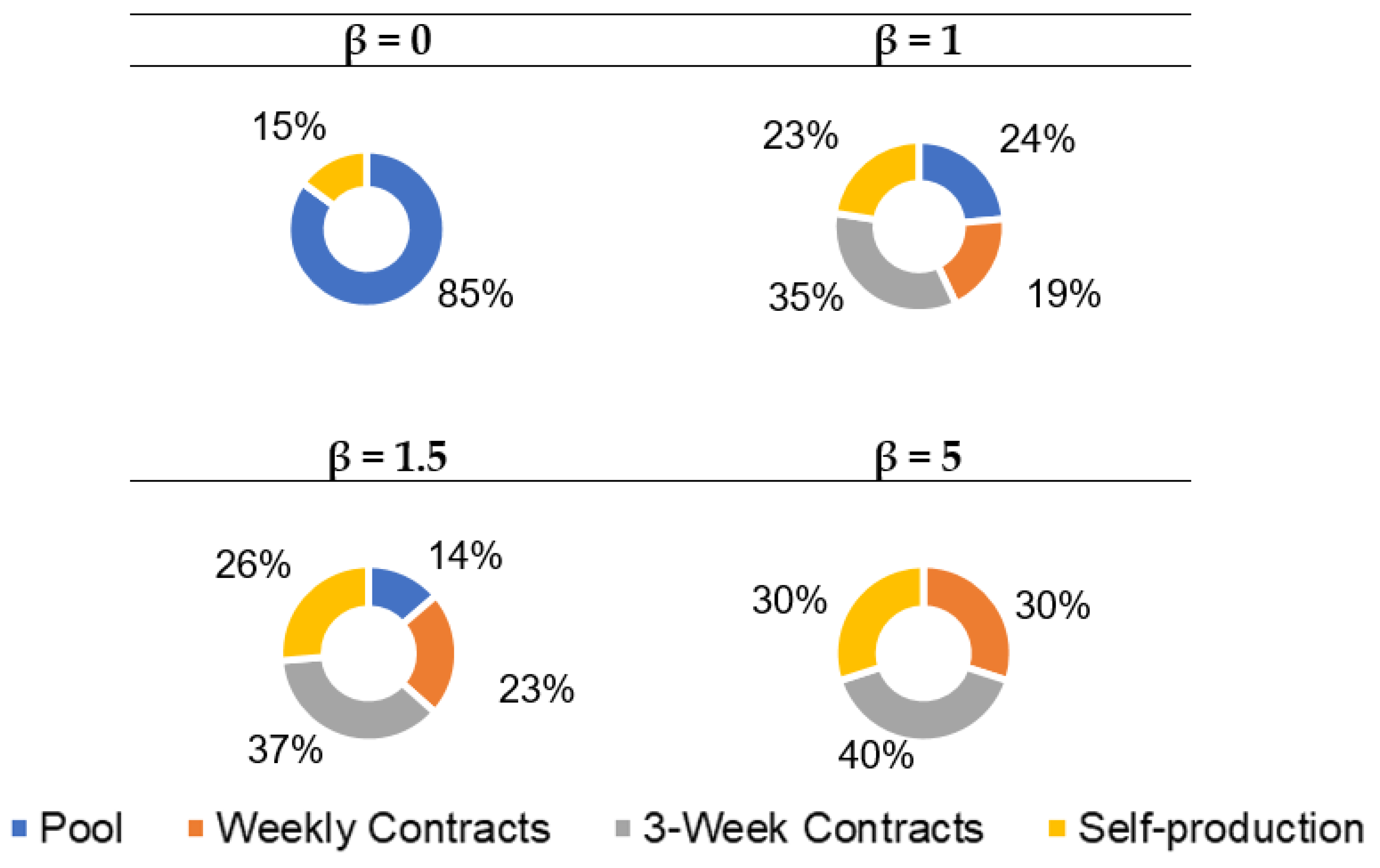
The objective function (OF) is defined though the weighted sum approach. The aim is to minimize the cost and risk of the portfolio, as in Equation (12). The weights used in the trade-off are defined through the value of the risk aversion factor β. This factor defines the decision-maker’s propensity towards risk. If β became equal to 0, the OF only considers the cost, representing 100% of OF, but if β takes the value 5, the weight associated to the cost term of the OF is 1/6 and the remaining related to the CVaR term, as 5/6.

The decision-maker aversion to long-term investment is characterized by the parameter, λ. This parameter aims to countering or favoring the production of self-generated energy based on the willingness to contract technology with high fixed costs and long-life span.

The objective function is defined in Equation (12), which minimizes the costs and risk, based on β values.

$$\min OF={\displaystyle \sum _w\left[{\pi }_w\times (C_w^P+\lambda \times C^G+C_w^C)+\beta \times CVaR\right]}$$

(12)

5. Data Collection and Parameter Estimation

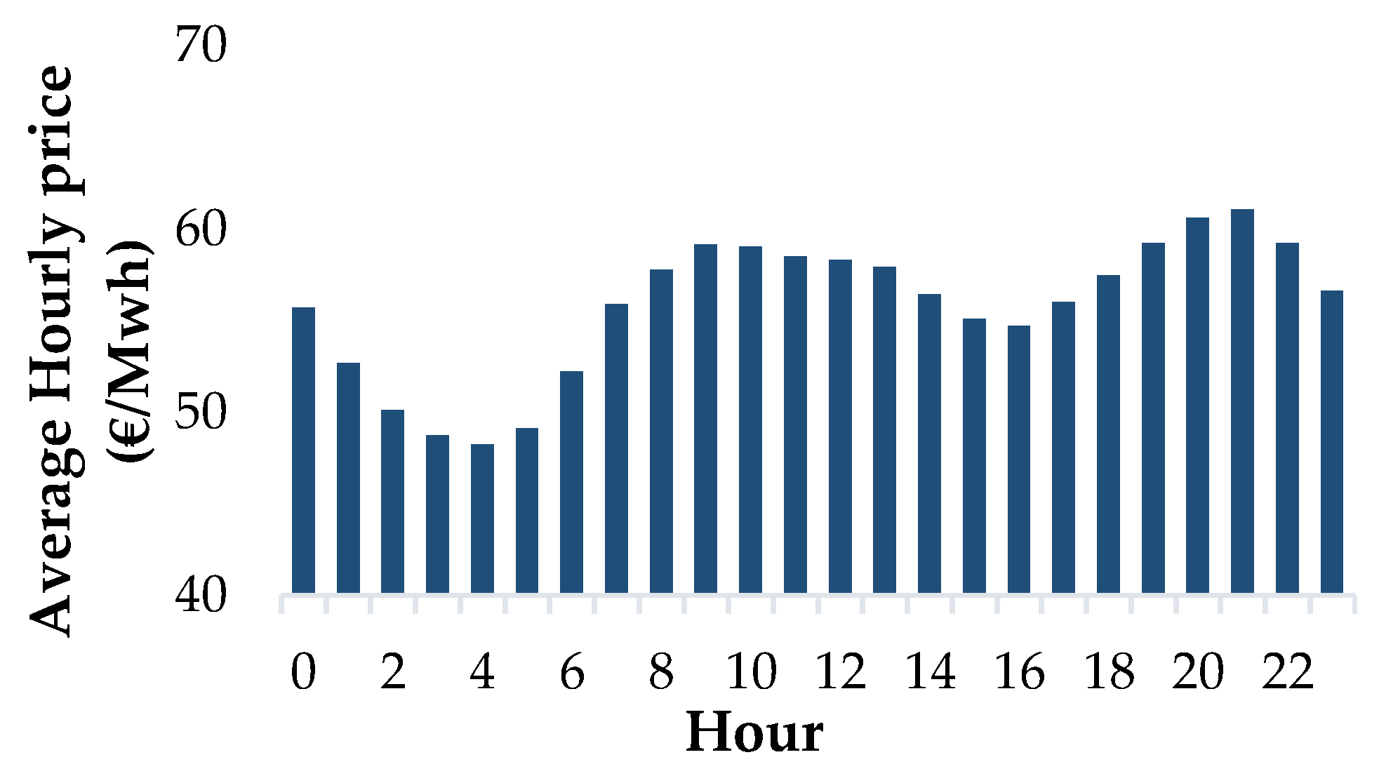
The electricity data explored in the work is from Iberian Operator database [7], over one year (September 2018 to August 2019). The year considered is representative of the Iberian electricity market. However, data screening was performed and 48 weeks is considered as a final sample. The seasonality and daily market variability are shown in Figure 2 and Figure 3.

Along the day, the spot market prices follow a high variability, triggering a very high data volume. To overcome this drawback, the hourly price values for the planning horizon over the 24 h in the 48 weeks, are averaged, as shown in Figure 2. The variability pattern in 24 h, denotes amplitude of 12.97 €, with its maximum of 61.02 € at 10 p.m. and a minimum of 48.23 € at 5 a.m. Considering this pattern, the data are categorized according to their average spot price, in three categories: valley, shoulder and peak hours. Those categories are associated to low, medium and high price, respectively. The valley hours define the hours with an average market value lower than 54 €, the peak define the hours with an average market value higher than 58 € and the shoulder define the hours with values in between. For 24 h, the following sets are defined:

Valley = {1, 2, 3, 4, 5, 6, 16}

Shoulder = {0, 7, 14, 15, 17, 18, 23}

Peak == {8, 9, 10, 11, 12, 13, 19, 20, 21, 22}

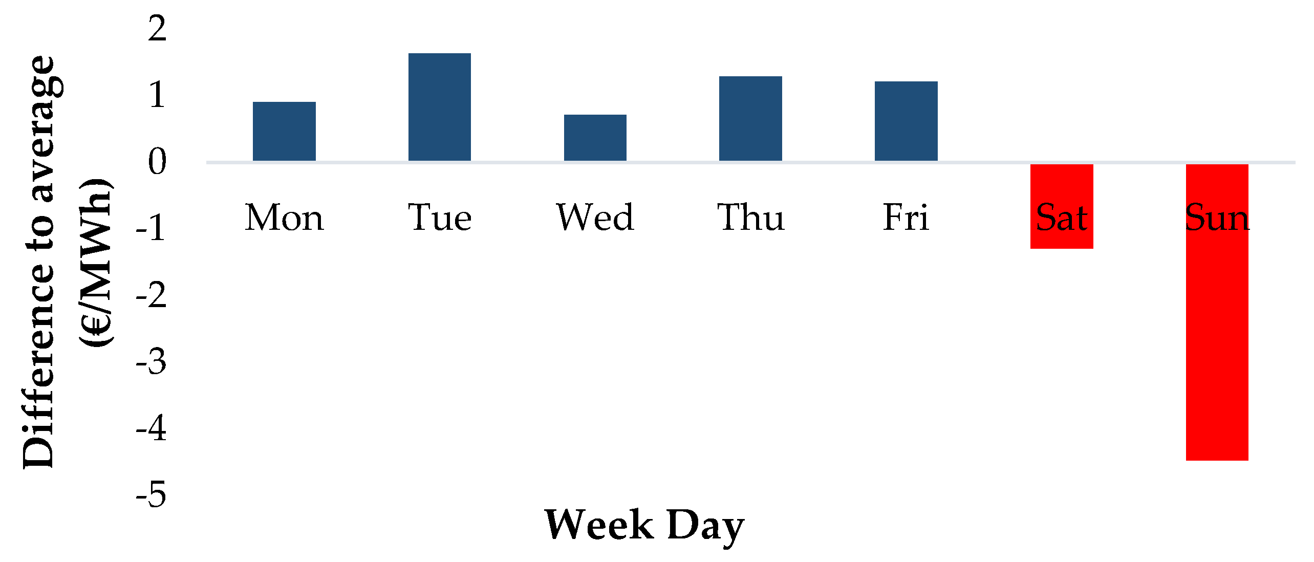
Other relevant data are to define the price for each day of the week, denoted from now on as, weekly day price. The weekly day price pattern results from the difference between the average price of each day of the week over the 48 weeks and the year average, shown in Figure 3. The weekly day pattern has its highest value on Tuesday and the lowest on Saturday and Sunday. This pattern is directly related with the electricity spot market prices variability.

5.1. Scenario Generation

In the scenario generation, a representative period of three weeks data are used to characterize the scenario: optimistic, pessimistic and expected week, as shown in

Table 1. Details of the weeks chosen to help in the scenario generation.

	Pessimistic Week	Expected Week	Optimistic Week
Maximum (€/MWh)	81.82	62.25	48.37
Minimum (€/MWh)	59.31	45.00	32.00
Average (€/MWh)	73.20	55.58	40.92
Standard Deviation	2.91	4.02	4.27

.

The weeks with the highest and lowest average price are chosen as pessimistic and optimistic scenario, respectively. The expected week takes the median of the average value.

In scenario tree, Figure 1, three branches leave each node, optimistic, expected and pessimistic, leading to 27 scenarios, for the three weeks. The probabilities for each scenario are based on the probability assigned to each branch over the 3 weeks. The scenarios’ probability characterization used the 48 weeks data, to consider yearly seasonality. Using the three weeks average values as a benchmark, the remaining weeks of the data set were divided in 3 sets, based on their average value. Each week is assigned to the set (characterized pessimist, average optimist), which as the closest value to the benchmark. The probabilities of each week shown in

Table 2. Benchmark Probabilities characterization: pessimist, expected and optimist.

	Pessimistic Week	Expected Week	Optimistic Week
Probability	0.15	0.58	0.27

, is the ration between the numbers of weeks in each set by the total set of 48 weeks. Finally, each scenario probability is obtained using the conditional probability and assuming independence between the events (multiplying the probabilities associated to the three branches leading to that scenario).

5.2. Forward Contract Data

The forward contract explores two different contracts: weekly and 3-week. Beyond that, a map of contract is also considered,

Table 3. Map of contracts.

	Valley	Shoulder	Peak	Base
Week 1	Contract 1	Contract 2	Contract 3	Contract 4
Week 2	Contract 5	Contract 6	Contract 7	Contract 8
Week 3	Contract 9	Contract 10	Contract 11	Contract 12
3-week	Contract 13	Contract 14	Contract 15	Contract 16

. The contracts will either set on the 24 h of the weeks they are settled on, denoted as base contracts or on one of the 3 sets of hours of the day, defined above: valley, shoulder and peak, denoted from now one as time-of-day contracts. Therefore 16 contracts are considered, as shown in Table 3.

Each contract is characterized in 4 blocks based on electricity prices and its electricity availability (maximum and minimum). Each block has 20 MWh available, which adds up to 80 MWh of electricity available per hour in each contract. If a contract is signed, it must have a minimum output of 20 MWh per hour.

The prices of the blocks are assigned to represent the behavior of a price-maker, similar methodology was followed by [50].

The prices assigned to the block 2 contract, is used as a baseline. Its values were defined considering the average price of each of these times in the spot market (e.g., the valley contracts have the lowest price per energy unit and peak contracts the highest). The prices in blocks 3 and 4 are increased by 5% and 10%, respectively, using the baseline. The baseline price was decreased by 2% to characterize the block 1. The price of the base contracts set is obtained through the prices of the valley, shoulder and peak contracts and the fraction of the day they represent. The resulting prices are shown in

Table 4. Weekly forward contract unit price (€/MWh).

	Block 1	Block 2	Block 3	Block 4
Valley	56.84	58	60.90	63.80
Shoulder	58.80	60	63	66
Peak	60.76	62	65.10	68.20
Base	59.05	60.25	63.26	66.28

.

The price of the second block for the 3-week contracts is determined by decreasing the values of the corresponding weekly contract in 2%. The price for the other blocks is calculated following the same methodology as the one used in the weekly contracts.

5.3. Self-Generation Facility

The self-generation case explores the implementation of a single renewable electricity source, with a levelized electricity price to characterize the fixed and variable costs. The levelized electricity price assumes the price per energy unit produced throughout the entire expected lifetime of the equipment. This way, it is possible to put the long-term investment into perspective, enabling a comparison with the electricity spot market prices, which allows an analysis of trade-off of the two.

Data were taken from study conducted by Fraunhofer Institute for Solar Energy Systems [51]. The installation of a PV technology is assumed. The levelized price is 35.5 €/MWh. This will be the price for the first block of energy. The following blocks’ prices are obtained by subsequently increasing in 10% the value of the original block, shown in

Table 5. Price of each block of the self-generation unit (€/MWh).

	Block 1	Block 2	Block 3	Block 4
Price Unit	35.5	39.5	42.6	63.8

. This method represents other costs that arise as the investment grows, e.g., cost of space for the PV panels. Each block has 15 MWh of energy available and there is a minimum of 15 MWh, if this source is chosen.

6. Case Studies

To illustrate and explore the model’s applicability of portfolio optimization three case studies are considered: case a) explores constant demand profile; case b) a cyclic daily demand comparison between nominal operating starting time and its optimization; case c) explores the weekly day price pattern over the two situations: with and without daily order optimization. To highlight each portfolio characteristics, different electricity demand profile is used. The confidence level used is 0.95. The general algebraic modeling system (GAMS) is used and the problems solved with an Intel Core i7 processor, until optimality is reached.

6.1. Case a): Constand Demand Profile

The portfolio characterization requires the aversion factor to long-term investment characterization. A constant hourly demand of 200 MWh, throughout the planning horizon is used.

6.1.1. Aversion Factor to Long-Term Generation Investment Value Characterization

The long-term generation investment is capital intensive and by nature has risk associated, requiring a deeper analysis for its characterization. The aversion factor value for long-term generation investment (λ) penalize or favor the use of self-generation facility. To diminish the impact this investment could have, considering a short-term decision-making model, this factor is multiplied by the cost obtained from the levelized electricity price, to become competitive between other options. Furthermore, a deeper analysis is undertake to define the λ value considering different risk postures, as shown in

Table 6. Weekly forward contract unit price (€/MWh).

	β
λ	0	1	1.5	2	5
1	60	60	60	60	60
1.3	30	45	52.65	60	60
1.6	0	0	0	15	15
2	0	0	0	0	0

, for different values of β and λ.

Table 6 illustrates how sensitive is the value of λ facing different risk postures. The cases where λ takes the extreme values (1 and 2) illustrate: on the former the electricity contracted from this source is at the maximum available value for all the values of risk aversion (60 €/MWh), which became very attractive compared to the other options; on the latter, however no self-generation investment is suggested for any risk posture, reflecting that the price is not competitive at all (0 €/MWh). For the cases where the factor is 1.3 and 1.6, the electricity generation are sensitive to different values of risk aversion. However, the model has higher sensitivity with λ =1.3, showing higher variability (from 30 to 60), which enables the self-generation facility more attractive to different risk postures. Therefore, the value of λ = 1.3 is selected to characterize the long-term generation investment.

6.1.2. Expected Cost vs. Conditional Value-at-Risk

To define the non-dominated solution and its Pareto front characterization, a trade-off between the conditional value-at-risk (CVaR) and the expected cost is explored, as shown in

Table 7. Expect cost and conditional value-at-risk (CVaR) trade-off for different risk postures (million €).

β	Expected Cost	CVaR
0	5.386	7.009
1	5.649	5.874
1.5	5.702	5.831
2	5.732	5.812
5	5.787	5.788

.

The solution for β = 0 reached the lowest expected cost and highest CVaR, while β = 5 reached lowest CVaR and highest expected cost. For β = 0 the OF term regarding risk is not taken into account, considering only expect cost minimization, while β = 5 the OF prioritizes the risk reduction. Hence, a reduction of the CVaR comes with an increase of the expected cost. It is relevant to notice β = 1, decrease 16.2% in the CVaR with a minor increase of the expected cost (4.88%).

6.1.3. Portfolio Evolution

The portfolio characterization makes use of different electricity supply options, with different prices and, different risk levels. The portfolio evolution for the 3 weeks contract over several levels of β is characterized in Figure 4 (figures are made by resorting the expected value of procurement over all scenarios). As Figure 4 illustrates the use of four types of electricity supply options: day-ahead market, self-production, weekly contracts and 3-week contracts in the portfolio characterization.

One of the most noticeable result is how the weekly and 3-week contracts increases as the value of β increases, reflecting conservative behavior (risk aversion) of the maker-decision, handling risk-free decision, triggering the increase of expected cost. Simultaneously, the self-generated electricity portfolio also increases, based on the same behavior of the decision-maker. The 3-week contracts are always higher than the weekly contracts. However, the electricity procured from the day-ahead market drops massively as the risk aversion increases, going from an 85% share, to 0% when β = 5.

6.1.4. Forward Contracts

Forward contracts and self-generation facility are able to hedge risk from the spot market. However, the risk behavior has impact in the selection of which and type of contacts for the portfolio. Specifically, for the forward contracts is necessary to analyze, how the contracting is developed from time-of-day contracts base, to weekly contracts, as the risk aversion increases.

The characterization of the several scenarios of forward contract over the sets, valley, shoulder and peak is shown in

Table 8. Forward contract: valley, shoulder and peak hour statistics (MWh).

β	Hours	Average forward Contracted Energy per Week	Energy from Time-of-Day	Energy from Base
0	Valley
	Shoulder	0	0	0
	Peak
1	Valley	78.9	25.6
	Shoulder	121.4	68.1	53.3
	Peak	118.5	65.1
1.5	Valley	86.8	25.7
	Shoulder	135.4	74.2	61.2
	Peak	132.3	71.1
5	Valley
	Shoulder	140	70.3	69.7
	Peak

. The results show as risk aversion increases, higher energy contracted for peak and shoulder hours increase compared with valley. Since this latter have higher spot market price, so contracts are done to hedge this risk.

Although, the behavior over the three sets are the similar for β = 0 and β = 5, none and the maximum forward contract, respectively. However, the forward contract increases as the risk aversion increases (β = 5). For the same values of β, the contact over shoulder and peak hours decrease, with its minimum in the base contact, while the valley denotes higher variability.

The electricity from forward contracts during the valley hours comes mainly from base contracts, while for shoulder and peak hours comes mainly from average forward energy/week and time-of-day contracts rather than from base. This behavior is justified due the price of the base contract is defined based on the prices of the 3 times of day. Although, it may be advantageous, since it can represent a lower price option in peak and shoulder hours, triggering an overpay in valley hours.

6.2. Case b): Cyclic Daily Demand over Optimized and Non-Optimized Starting Time

This case study follows a cyclic daily demand (24-h cycle) of a multipurpose batch plant [52] campaign production, which repeats itself continuously for the campaign duration. As previously identified and characterized the spot market prices seasonality over the hour of the day (Valley, shoulder and peak hours) is explored in this context.

The aim is to analyze how the facility can take advantage from daily seasonality. Case b) is split into two smaller situations: the starting time of the cycle is optimized vs. non optimize (the starting time is defined at hour 0 of the series). The comparison and results illustrate the impact on the trade-off between expect cost vs. risk. A mixed demand pattern is used for the cycle, with minimum, maximum and average consumption of 170 MWh, of 250 MWh and of 200 MWh, respectively.

6.2.1. Starting Time Formulation

To formulate this behavior the aforementioned formulation is extended, with equations Equations (13) and (14). Equation (13) guarantees that only one starting time is chosen, while Equation (14) selects the right schedule to be used considering the energy balance Equation (8).

An extended formulation considers a starting times index, θ and parameter for the demand, where the demand profiles along the hours, t, is shifted for all the possible starting times θ, ${\mathrm{ND}}_{\mathrm{t},\mathsf{\theta }}$. The binary variable became $s_{\theta }$=1, if θ is the starting time chosen, 0 otherwise. The parameter $D_{d,t}$ of Equation (8) became $D_t$.

$${\displaystyle \sum _{\theta }^{N_{\theta }}{s}_{\theta }^s}=1.$$

(13)

$${\displaystyle \sum _{\theta }^{N_{\theta }}(s_{\theta }^s\times N{D}_{t,\theta }})=D_t\forall t\in N_t$$

(14)

6.2.2. Expect Cost vs. CVaR Comparison

The Pareto front characterization and its results for with and without starting time optimization are shows in Figure 5 and

Table 9. Stating time optimization vs. non-optimization.

	Starting-Time Optimization			Non Optimization
$\mathit{\beta }$	Expected Cost (Million €)	CVaR (Million €)	Starting Time	Expected Cost (Million €)	CVaR (Million €)
0	5.364	6.994	7 h	5.414	7.025
1	5.576	5.925	6 h	5.644	5.940
1.5	5.643	5.878	8 h	5.703	5.893
2	5.689	5.851	8 h	5.720	5.884
5	5.705	5.846	8 h	5.746	5.873

, respectively.

The starting time optimization has a lower expected cost than the non-optimized, for the same values of β, as shown in Figure 5. However, the trade-off between the expected cost and the risk shows the starting time varies depending on the risk behavior. If the decision-maker takes β = 0, the starting time is 7 h. However, for β = 1, the optimized starting time is 6 h and, for the remains values of β = 1.5, 2, 5 is 8 h. As in previous analyzes, the expected cost increases in both scenarios with the increment of the risk aversion factor and the CVaR decreases.

6.2.3. Procurement Analyses: Valley, Shoulder and Peak Hours

The portfolio characterization over the three sets (valley, shoulder and peak) and its comparison between with or without start time optimization is shown in

Table 10. Total procurement on valley, shoulder and peak hours for different risk aversion factors with and without starting-time optimization.

	Non-Optimization (MWh)			Optimization (MWh)
β	Valley	Shoulder	Peak	Valley	Shoulder	Peak
0	26,040	30,240	44,520	33,180	28,560	39,060
1	26,040	30,240	44,532	33,180	28,140	39,480
1.5	26,040	30,240	44,532	32,340	29,820	38,640
2	26,040	30,240	44,535	32,340	29,832	38,640
5	25,373	29,573	43,583	33,007	30,505	39,593

. Analyzing the pattern from the sets in non-optimized versus optimized shows: an increase of energy procurement in the valley set in the optimized rather and non-optimized and, an opposite behavior decreases in the shoulder and peak sets. This behavior is justified by the starting time optimization avoids matching the hours with higher demand (peak hours) and rather takes advantage from the valley hours. This resulted on a drop of 12.24% in the electricity procurement in peak hours, on average from every value of β and an increase of 26.5% in the valley hours.

6.3. Case c): Weekly Optimization

The third case explores the price pattern of each day of the week, week seasonality (Figure 3). The scheduling of activities is optimized according the trade-off between minimization of expected cost and risk. However, this case uses a representative sample of seven days of energy demand, denote further on, as series, which are allocated to an optimal day of the week.

Seven representative days of demand are randomly selected to be scheduled within the week, defined in

Table 11. Statistics on 7-day demand profiles (MWh).

	1st	2nd	3rd	4th	5th	6th	7th
Mean	180	220	250	270	250	220	250
Std. Dev.	10	20	20	20	30	40	40
Max	193	256	296	318	324	305	334
Min	263	181	211	228	130	136	185
CV (%)	5.55	9.09	8.00	7.40	12	18.2	16.0

. Based on the 24 h information of these days the demand profiles are characterized. Its statistics are shown in Table 11. The 6th series has the highest variability (CV=18.2%), while the 1th the lowest. Being the 7th and the 4th series with the highest maximum values. The schedule defined is repeated for the 3 weeks under study.

6.3.1. Weekly Optimization

For the weekly optimization and based on aforementioned formulation, the formulation is extended with constraints Equations (15)–(17). Equation (15) guarantees that only one-day demand profile (from Table 11) is assigned to each day of the week, through the binary $s_{d,\lambda }^s$. Equation (16) guarantees that all day demand profiles are assigned to a day of the week. Equation (17) defines the final demand profile.

A new index, γ, is used as an alias of d; the parameter, ${\mathrm{EED}}_{\mathrm{t},\mathsf{\gamma }}$, characterize the 7-day profiles. The demand profile, $D_{d,t}$, is obtained in Equation (17) to be used in Equation (8).

$${\displaystyle \sum _{\gamma }{s}_{d,\lambda }^s}=1\forall d\in N_d$$

(15)

$${\displaystyle \sum _d{s}_{d,\lambda }^s}=1\forall \gamma \in N_{\gamma }$$

(16)

$$D_{d,t}={\displaystyle \sum _{\gamma }{s}_{d,\gamma }^s}\times EE{D}_{t,\gamma }\forall d\in N_d,\forall t\in N_t$$

(17)

6.3.2. Pareto Front Characterization

The Pareto front is defined for with and without order optimization, followed by the day order scheduling analysis, in Figure 6 and

Table 12. Day order scheduling results.

β	Mon	Tue	Wed	Thu	Fri	Sat	Sun
0	2nd	1st	6th	5th	3rd	7th	4th
1	3rd	6th	1st	2nd	5th	7th	4th
1.5	2nd	6th	1st	3rd	5th	7th	4th
2	6th	5th	1st	3rd	2nd	7th	4th
5	4th	5th	1st	7th	2nd	6th	3rd

, respectively.

Both situations have a similar behavior. The expected cost increases and the CVaR decreases with the increase aversion towards risk (β). However, the order optimization allows more favorable trade-offs between the two objective functions, for every β.

6.3.3. Day Order Scheduling Analysis

The day order optimization considers how the price seasonality of the day of the week (Figure 3), impact in the energy purchase, based on data from Table 11. The analysis is performed for several aversion to risk patterns and the results are shown in Table 2.

Figure 3 identifies the days with lower electricity prices are: Sunday, Wednesday and Saturday, respectively. The result of the weekly day optimization in Table 12, shows the impact the daily price seasonality has. All risk aversion values, except β = 5, the day-series for Saturday and Sunday are the 7th and 4th, respectively. These results from the 4th and 7th series have the highest and second higher mean value, being assigned to the days with the lowers electricity price, Sunday and Saturday, respectively. The remaining days of the week, from Monday to Friday, shows a difference price pattern, although less relevant (Figure 3), where the days’ difference to average was very similar.

7. Conclusions

This work proposes a mixed integer linear formulation for the energy portfolio optimization problem for large consumer in a buyer perspective. A multi-objective approach is explored to deploy several options to the decision-maker based on its risk pattern. A weighted sum formulation is presented for the expected cost and risk minimization. The binary variables define the procurement decisions and the continuous variables define the electricity procured, cost of each electricity supplier options, as well as the value of the CVaR.

The Iberian electricity market is considered as a case study. The data analysis and screening are developed and are highlighted and used in the cases studies for price seasonality, weekly and daily bases. The electricity supply options explored for the portfolio characterization are pool market, forward contract and self-generation.

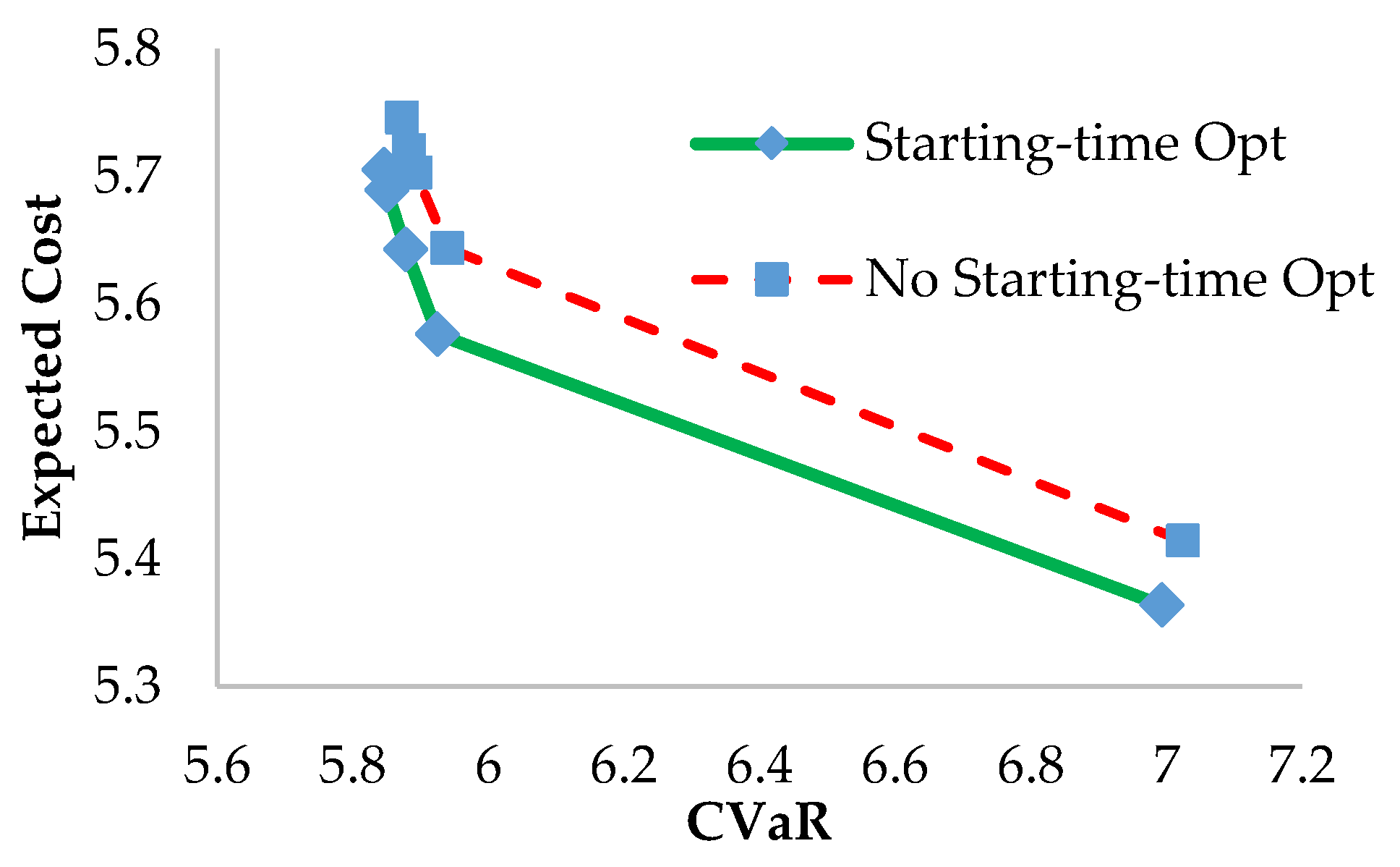
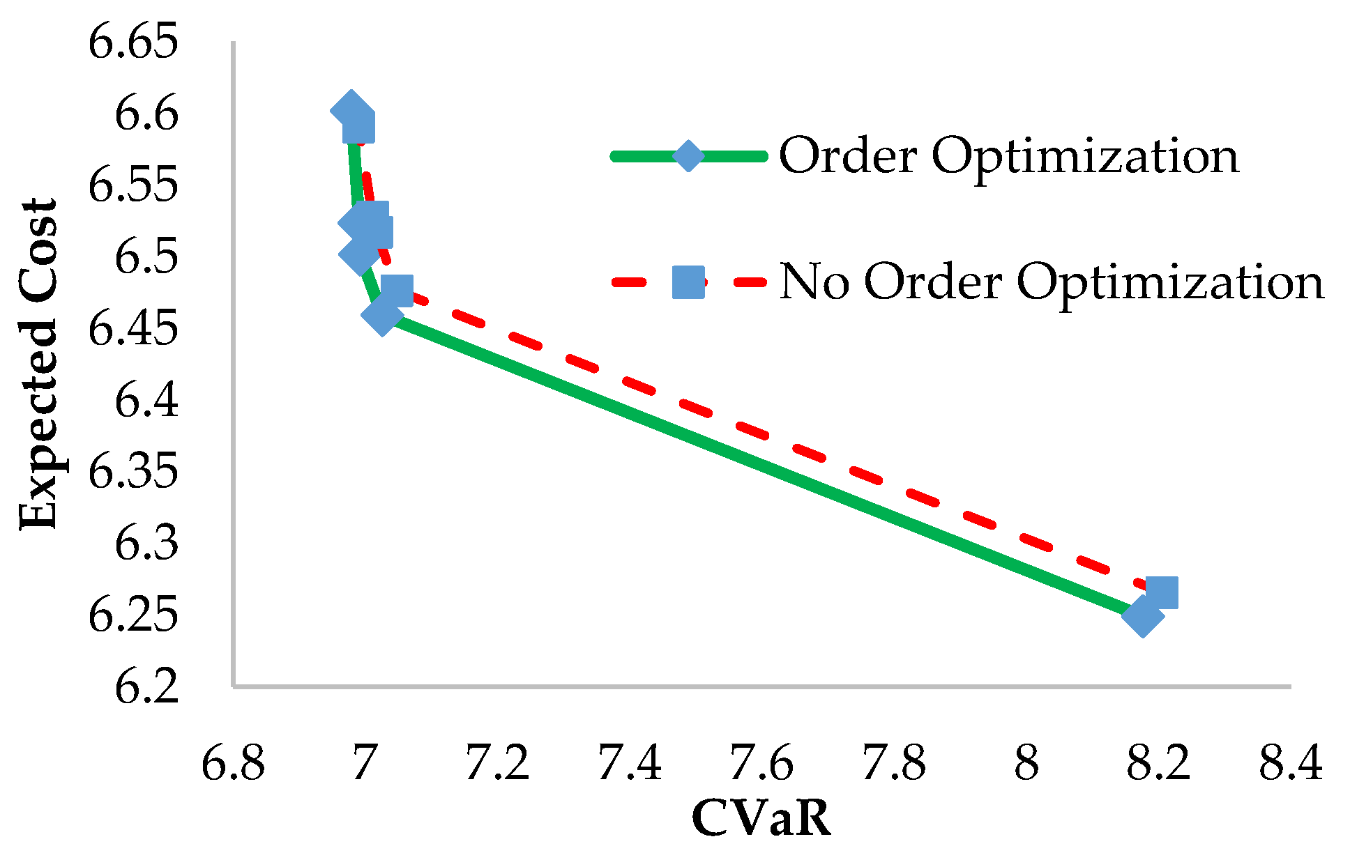
The portfolio characterization and the decision-maker behavior towards to risk is developed exploring three cases. Case a) uses constant demand profile; case b) explores manufacturing aspect, considering a cyclic daily demand and a comparison between nominal operating starting time and its optimization is developed, while case c) explores the weekly day price seasonality. In all cases different values of the risk aversion factor are explored.

Some practical guidelines may be drawn from the results. From case a) the pool market procurement reveals more suitable for decision-maker with pattern taker to risk, while risk averted decision-maker prefer forward contracts and self-generated energy. These different postures lead to a higher CVaR and lower expected cost for the risk taker decision-maker and lower CVaR and higher expected cost for the risk averted decision-maker.

The seasonality effect is explored in cases b) and c). The results from case b), which consider the hour seasonality, avoid the high price hours and favor the low-price hours. In case c) the week seasonality is considered and the tendency is favoring low price days rather than high price. The advantage from using the hour price seasonality (case b) shows better results in terms of objective than case c). As a guideline for the decision-maker, the demand allocation considering the hours of the day, reveled more effective in price reduction than solely paying attention to the day of the week.

Three aspects should be considered as further work. The self-generated energy should be explored not only from the buyers, but also the seller perspective. The use of converting temporarily the electricity in some other form, taking advantage from the low price, so as to be used in the short term. In addition, data analytics approaches, to deal with more detailed information and real-time optimization.

References

1. Pérez Odeh, R.P.; Watts, D.; Negrete-Pincetic, M. Portfolio applications in electricity markets review: Private investor and manager perspective trends. Renew. Sustain. Energy Rev. 2018, 81, 192–204. [Google Scholar] [CrossRef]
2. Pérez Odeh, R.P.; Watts, D.; Flores, Y. Planning in a changing environment: Applications of portfolio optimisation to deal with risk in the electricity sector. Renew. Sustain. Energy Rev. 2018, 82, 3808–3823. [Google Scholar] [CrossRef]
3. Kaleta, M.; Toczyłowski, E. Restriction techniques for the unit-commitment problem with total procurement costs. Energy Policy 2008, 36, 2439–2448. [Google Scholar] [CrossRef]
4. Toczyłowski, E.; Zoltowska, I. A new pricing scheme for a multi-period pool-based electricity auction. Eur. J. Oper. Res. 2009, 197, 1051–1062. [Google Scholar] [CrossRef]
5. Huisman, R.; Mahieu, R. Regime jumps in electricity prices. Energy Econ. 2003, 25, 425–434. [Google Scholar] [CrossRef] [Green Version]
6. Huisman, R.; Mahieu, R.; Schlichter, F. Electricity portfolio management: Optimal peak/off-peak allocations. Energy Econ. 2009, 31, 169–174. [Google Scholar] [CrossRef] [Green Version]
7. OMIE. Market Results of the Iberian Power Spot Exchange, Iberian Market Operator, Spanish Pool. 2019. Available online: http://www.omie.es/files/flash/ResultadosMercado.html# (accessed on 1 January 2020).
8. Babonneau, F.; Caramanis, M.; Haurie, A. A linear programming model for power distribution with demand response and variable renewable energy. Appl. Energy 2016, 181, 83–95. [Google Scholar] [CrossRef]
9. Thombs, R.P. When democracy meets energy transitions: A typology of social power and energy system scale. Energy Res. Soc. Sci. 2019, 52, 159–168. [Google Scholar] [CrossRef]
10. Kokkinos, K.; Karayannis, V.; Moustakas, K. Circular bio-economy via energy transition supported by Fuzzy Cognitive Map modeling towards sustainable low-carbon environment. Sci. Total Environ. 2020, 721, 137754. [Google Scholar] [CrossRef]
11. Falcone, P.M.; Lopolito, A.; Sica, E. Instrument mix for energy transition: A method for policy formulation. Technol. Forecast. Soc. Chang. 2019, 148, 119706. [Google Scholar] [CrossRef]
12. Owen, R.; Brennan, G.; Fergus Lyon, F. Enabling investment for the transition to a low carbon economy: Government policy to finance early stage green innovation. Curr. Opin. Environ. Sustain. 2018, 31, 137–145. [Google Scholar] [CrossRef]
13. Falcone, P.M. Tourism-Based Circular Economy in Salento (South Italy): A SWOT-ANP Analysis. Soc. Sci. 2019, 8, 216. [Google Scholar] [CrossRef] [Green Version]
14. Cui, Y.; Geng, Z.; Zhu, Q.; Han, Y. Multi-objective optimization methods and application in energy saving. Energy 2017, 125, 681–704. [Google Scholar] [CrossRef]
15. Chiandussi, G.; Codegone, M.; Ferrero, S.; Varesio, F.E. Comparison of multi-objective optimization methodologies for engineering applications. Comput. Math. Appl. 2012, 63, 912–942. [Google Scholar] [CrossRef] [Green Version]
16. Sawik, B. Survey of multi-objective portfolio optimization by linear and mixed integer programming. In Applications of Management Science; Lawrence, K.D., Kleinman, G., Eds.; Emerald Group Publishing Limited: Bingley, UK, 2013; Volume 16, pp. 55–79. [Google Scholar]
17. Sawik, B. Weighted-Sum Approach for Bi-Objective Optimization of Fleet Size with Environmental Aspects. In Applications of Management Science; Lawrence, K.D., Kleinman, G., Eds.; Emerald Group Publishing Limited: Bingley, UK, 2018; Volume 19, pp. 101–116. [Google Scholar]
18. Chankong, V.; Haimes, Y.Y. Multiobjective Decision Making: Theory and Methodology; Courier Dover Publications: Mineola, NY, USA, 2008. [Google Scholar]
19. Caramia, M.; Dell’Olmo, P. Multi-Objective Management in Freight Logistics: Increasing Capacity, Service Level and Safety with Optimization Algorithms; Springer Science & Business Media: London, UK, 2008. [Google Scholar]
20. Pindoriya, N.M.; Singh, S.N.; Singh, S.K. Multi-objective mean–variance–skewness model for generation portfolio allocation in electricity markets. Electr. Power Syst. Res. 2010, 80, 1314–1321. [Google Scholar] [CrossRef]
21. Liu, M.; Wu, F.F. Portfolio optimization in electricity markets. Electr. Power syst. Res. 2007, 77, 1000–1009. [Google Scholar] [CrossRef]
22. Feng, D.; Gan, D.; Zhong, J.; Ni, Y. Supplier asset allocation in a pool-based electricity market. IEEE Trans. Power Syst. 2007, 22, 1129–1138. [Google Scholar] [CrossRef] [Green Version]
23. Markowitz, H. Portfolio selection. J. Financ. 1952, 7, 77–91. [Google Scholar]
24. Sawik, B. Downside Risk Approach for Multi-Objective Portfolio Optimization. In Operations Research Proceedings 2011; Klatte, D., Lüthi, H.-J., Schmedders, K., Eds.; Springer: Berlin/Heidelberg, Germany, 2012; pp. 191–196. [Google Scholar]
25. Sawik, B. Triple-Objective Models for Portfolio Optimisation with Symmetric and Percentile Risk Measures. Int. J. Logist. Syst. Manag. 2016, 25, 96–107. [Google Scholar] [CrossRef]
26. Chong, J.; Jin, Y.; Phillips, M. The Entrepreneur’s Cost of Capital: Incorporating Downside Risk in the Buildup Method; MacroRisk Analytics Working Paper Series; MacroRisk Analytics: Pasadena, CA, USA, 2013; p. 5. [Google Scholar]
27. Rockafellar, R.T.; Uryasev, S. Optimization of conditional value-at-risk. J. Risk 2000, 2, 21–42. [Google Scholar] [CrossRef] [Green Version]
28. Lim, A.E.; Shanthikumar, J.G.; Vahn, G.Y. Conditional value-at-risk in portfolio optimization: Coherent but fragile. Oper. Res. Lett. 2011, 39, 163–171. [Google Scholar] [CrossRef]
29. Sarykalin, S.; Serraino, G.; Uryasev, S. Value-at-risk vs. conditional value-at-risk in risk management and optimization. In State-of-the-Art Decision-Making Tools in the Information-Intensive Age; Informs: Catonsville, MD, USA, 2008; pp. 270–294. [Google Scholar]
30. Sawik, B. A Three Stage Lexicographic Approach for Multi-Criteria Portfolio Optimization by Mixed Integer Programming. Przeglad Elektrotechniczny 2008, 84, 108–112. [Google Scholar]
31. Sawik, B. Bi-Criteria Portfolio Optimization Models with Percentile and Symmetric Risk Measures by Mathematical Programming. Przeglad Elektrotechniczny 2012, 88, 176–180. [Google Scholar]
32. Sawik, B. Conditional Value-at-Risk vs. Value-at-Risk to Multi-Objective Portfolio Optimization. In Applications of Management Science; Lawrence, K.D., Kleinman, G., Eds.; Emerald Group Publishing Limited: Bingley, UK, 2012; Volume 15, pp. 277–305. [Google Scholar]
33. Kizys, R.; Juan, A.A.; Sawik, B.; Calvet, L. A Biased-Randomized Iterated Local Search Algorithm for Rich Portfolio Optimization. Appl. Sci. (Basel) 2019, 9, 3509. [Google Scholar]
34. Uryasev, S. Conditional value-at-risk: Optimization algorithms and applications. In Proceedings of the IEEE/IAFE/INFORMS 2000 Conference on Computational Intelligence for Financial Engineering (CIFEr) (Cat. No. 00TH8520), New York, NY, USA, 28 March 2000; pp. 49–57. [Google Scholar]
35. deLlano-Paz, F.; Calvo-Silvosa, A.; Antelo, S.I.; Soares, I. Energy planning and modern portfolio theory: A review. Renew. Sustain. Energy Rev. 2017, 77, 636–651. [Google Scholar] [CrossRef]
36. Wu, Y.; Xu, C.; Ke, Y.; Tao, Y.; Li, X. Portfolio optimization of renewable energy projects under type-2 fuzzy environment with sustainability perspective. Comput. Ind. Eng. 2019, 133, 69–82. [Google Scholar] [CrossRef]
37. Costa, O.L.; de Oliveira Ribeiro, C.; Rego, E.E.; Stern, J.M.; Parente, V.; Kileber, S. Robust portfolio optimization for electricity planning: An application based on the Brazilian electricity mix. Energy Econ. 2017, 64, 158–169. [Google Scholar] [CrossRef]
38. Chen, Y.; Trifkovic, M. Optimal scheduling of a microgrid in a volatile electricity market T environment: Portfolio optimization approach. Appl. Energy 2018, 226, 703–712. [Google Scholar] [CrossRef]
39. Hu, J.; Harmsen, R.; Crijns-Graus, W.; Worrell, E. Geographical optimization of variable renewable energy capacity in China using modern portfolio theory. Appl. Energy 2019, 253, 113614. [Google Scholar] [CrossRef]
40. Lorca, A.; Prina, J. Power portfolio optimization considering locational electricity prices and risk management. Electr. Power Syst. Res. 2014, 109, 80–89. [Google Scholar] [CrossRef]
41. Algarvio, H.; Lopes, F.; Sousa, J.; Lagarto, J. Multi-agent electricity markets: Retailer portfolio optimization using Markowitz theory. Electr. Power Syst. Res. 2017, 148, 282–294. [Google Scholar] [CrossRef]
42. Garcia, R.C.; González, V.; Contreras, J.; Custodio, J.E. Applying modern portfolio theory for a dynamic energy portfolio allocation in electricity markets. Electr. Power Syst. Res. 2017, 150, 11–23. [Google Scholar] [CrossRef]
43. Gökgöz, F.; Atmaca, M.E. Portfolio optimization under lower partial moments in emerging electricity markets: Evidence from Turkey. Renew. Sustain. Energy Rev. 2017, 67, 437–449. [Google Scholar] [CrossRef]
44. Bao, X.; Zhao, W.; Wang, X.; Tan, Z. Impact of policy mix concerning renewable portfolio standard and emissions trading on electricity market. Renew. Energy 2019, 135, 761–774. [Google Scholar] [CrossRef]
45. Lucheroni, C.; Mari, C. Risk shaping of optimal electricity portfolios in the stochastic LCOE theory. Comput. Oper. Res. 2018, 96, 374–385. [Google Scholar] [CrossRef]
46. Park, S.Y.; Yun, B.Y.; Yun, C.Y.; Lee, D.H.; Choi, D.G. An analysis of the optimum renewable energy portfolio using the bottom–up model: Focusing on the electricity generation sector in South Korea. Renew. Sustain. Energy Rev. 2016, 53, 319–329. [Google Scholar] [CrossRef]
47. Wang, J.; Li, L. Sustainable energy development scenario forecasting and energy saving policy analysis of China. Renew. Sustain. Energy Rev. 2016, 58, 718–724. [Google Scholar] [CrossRef]
48. Conejo, A.J.; Carrión, M.; Morales, J.M. Decision Making under Uncertainty in Electricity Markets; Springer: New York, NY, USA, 2010; Volume 1. [Google Scholar]
49. Terradez, M.; Kizys, R.; Juan, A.A.; Debon, A.M.; Sawik, B. Risk Scoring Models for Trade Credit in Small and Medium Enterprises. In Springer Proceedings in Mathematics & Statistics; Kitsos, C.P., Oliveira, A., Rigas, A., Gulati, S., Eds.; Springer: Berlin/Heidelberg, Germany, 2015; Volume 16, pp. 349–360. [Google Scholar]
50. Nojavan, S.; Nourollahi, R.; Pashaei-Didani, H.; Zare, K. Uncertainty-based electricity procurement by retailer using robust optimization approach in the presence of demand response exchange. Int. J. Electr. Power Energy Syst. 2019, 105, 237–248. [Google Scholar] [CrossRef]
51. Kost, C.; Shammugam, S.; Julch, V.; Nguyen, H.-T.; Schlegl, T. Levelized Cost of Electricity Renewable Energy Technologies; Fraunhofer Institute for Solar Energy Systems ISE: Freiburg, Germany, 2018. [Google Scholar]
52. Pinto-Varela, T.; Barbosa-Povoa, A.P.F.; Novais, A.Q. Design and scheduling of periodic multipurpose batch plants under uncertainty. Ind. Eng. Chem. Res. 2009, 48, 9655–9670. [Google Scholar] [CrossRef]
Figure 1. Scenario tree.
Energies 13 02249 g001
Figure 2. Average hourly price of electricity.
Energies 13 02249 g002
Figure 3. Difference between the year average and each day of the week.
Energies 13 02249 g003
Figure 4. Portfolio evolution.
Energies 13 02249 g004
Figure 5. Efficient frontier for case b (million €).
Energies 13 02249 g005
Figure 6. Efficient Frontier for case c (million €).
Energies 13 02249 g006