A Critical Review of Wind Power Forecasting Methods—Past, Present and Future


Abstract
:1. Introduction
2. Classification of Wind Power Forecasting
2.1. Prediction Horizons
2.2. Prediction Methodologies
2.2.1. Persistence Methods
2.2.2. Physical Methods
2.2.3. Statistical Methods
Time Series Models
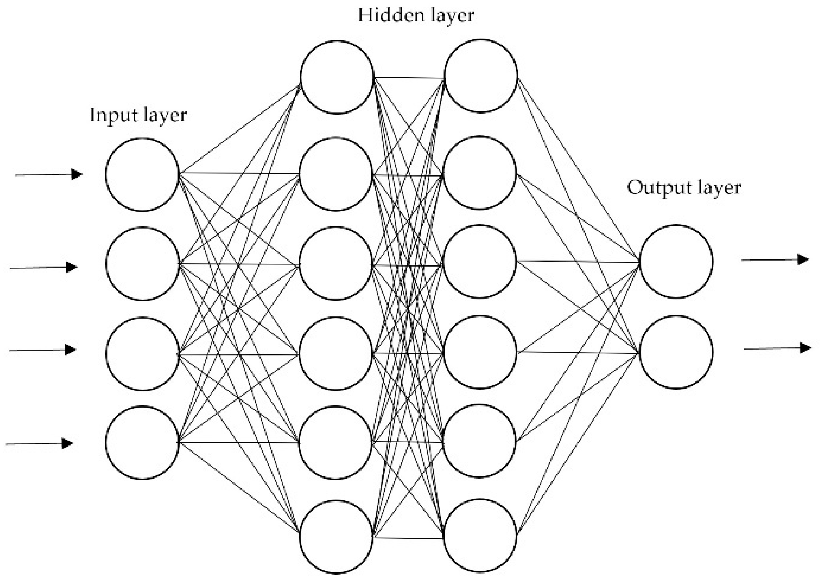
ANNs
2.2.4. Hybrid Approach
3. Factors to Compare Different Methods
3.1. Accuracy
3.2. Computational Time
4. Performance Evaluation in Wind Power Forecasting
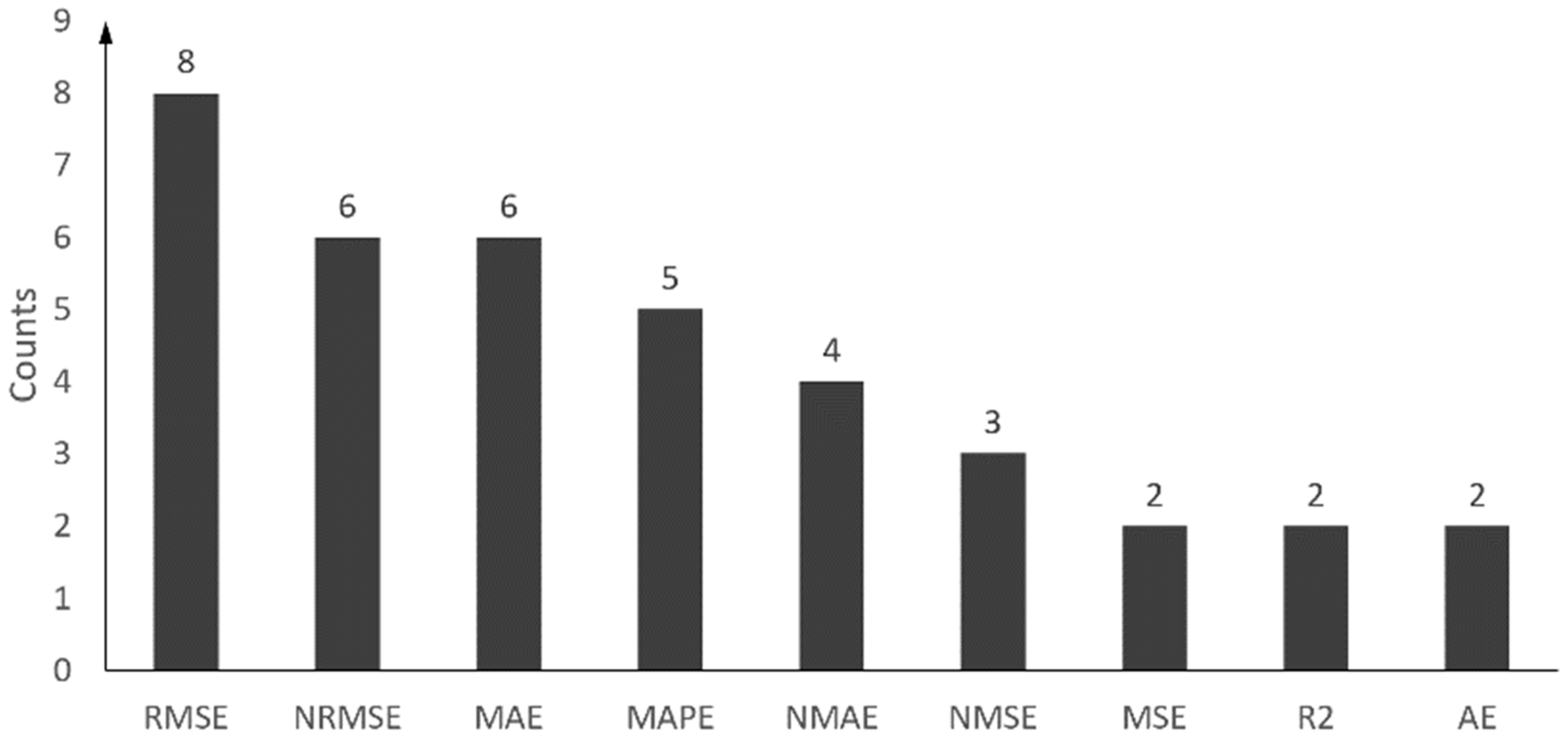
4.1. Error Measurements
4.1.1. Normalised Error
4.1.2. Normalised Mean Bias Error (NMBE)
4.1.3. Normalised Mean Absolute Error (%)
4.1.4. Normalised Root Mean Square Error (%)
4.1.5. Mean Squared Logarithmic Error (MSLE)
4.1.6. R-Square (R2)
4.1.7. Explained Variance Score (EVS)
4.1.8. Median Absolute Error (MAE)
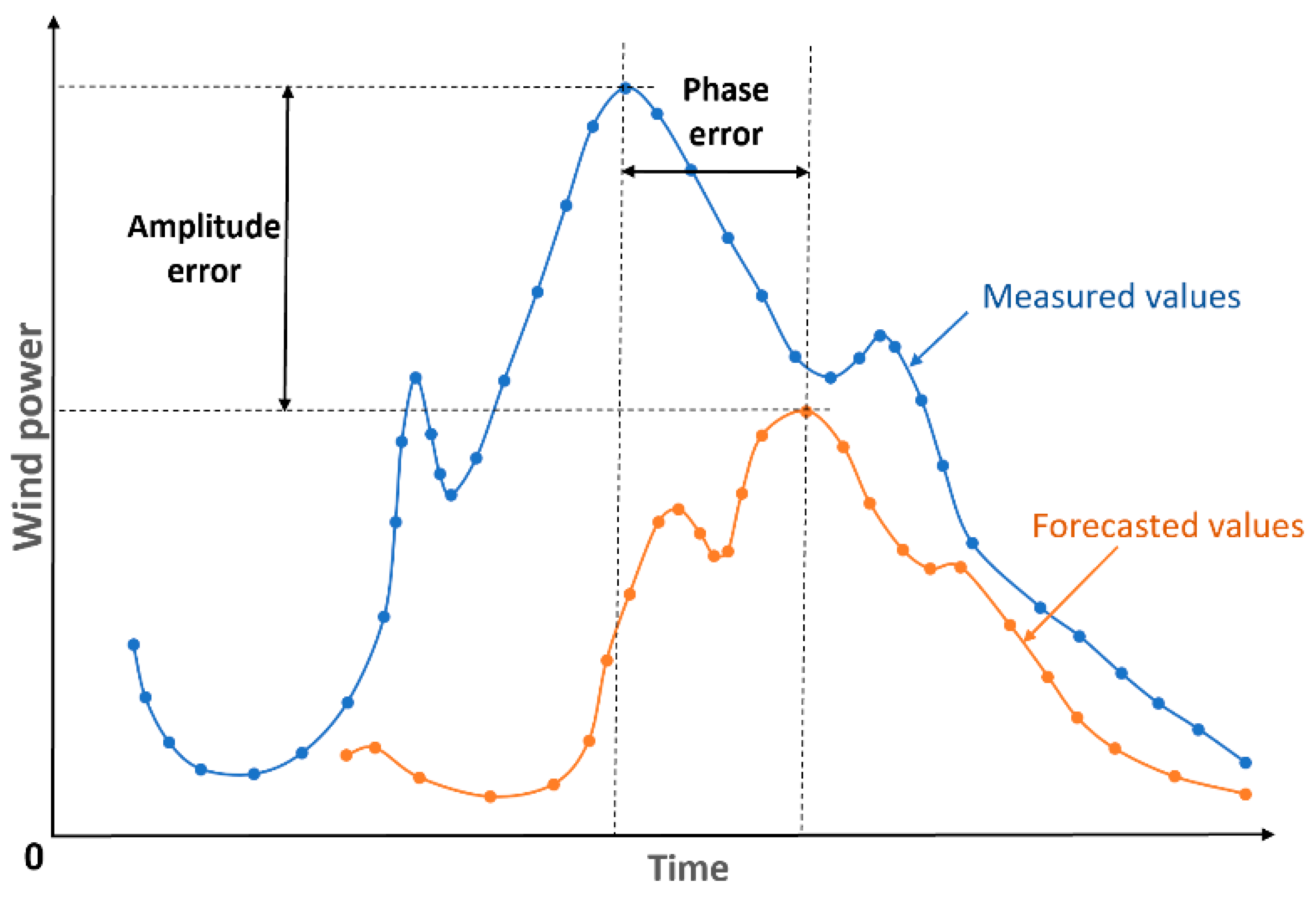
4.2. The Amplitude and Phase Error
4.3. Statistical Error Distribution
5. Enhancement of Predictive Accuracy
5.1. Kalman Filtering
5.2. Outlier Detection
5.3. Optimal Combinations
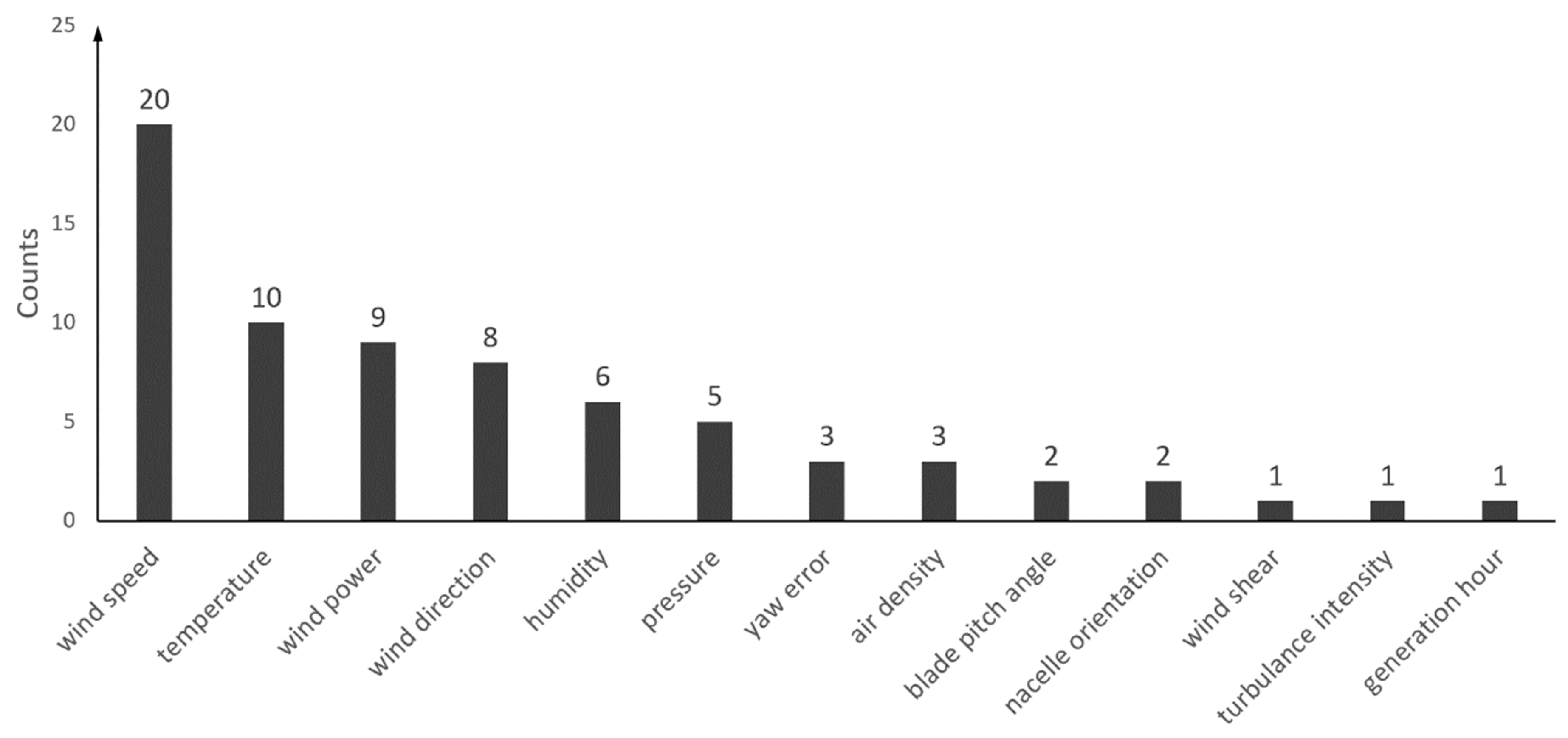
5.4. Input Parameters
5.5. Statistical Downscaling
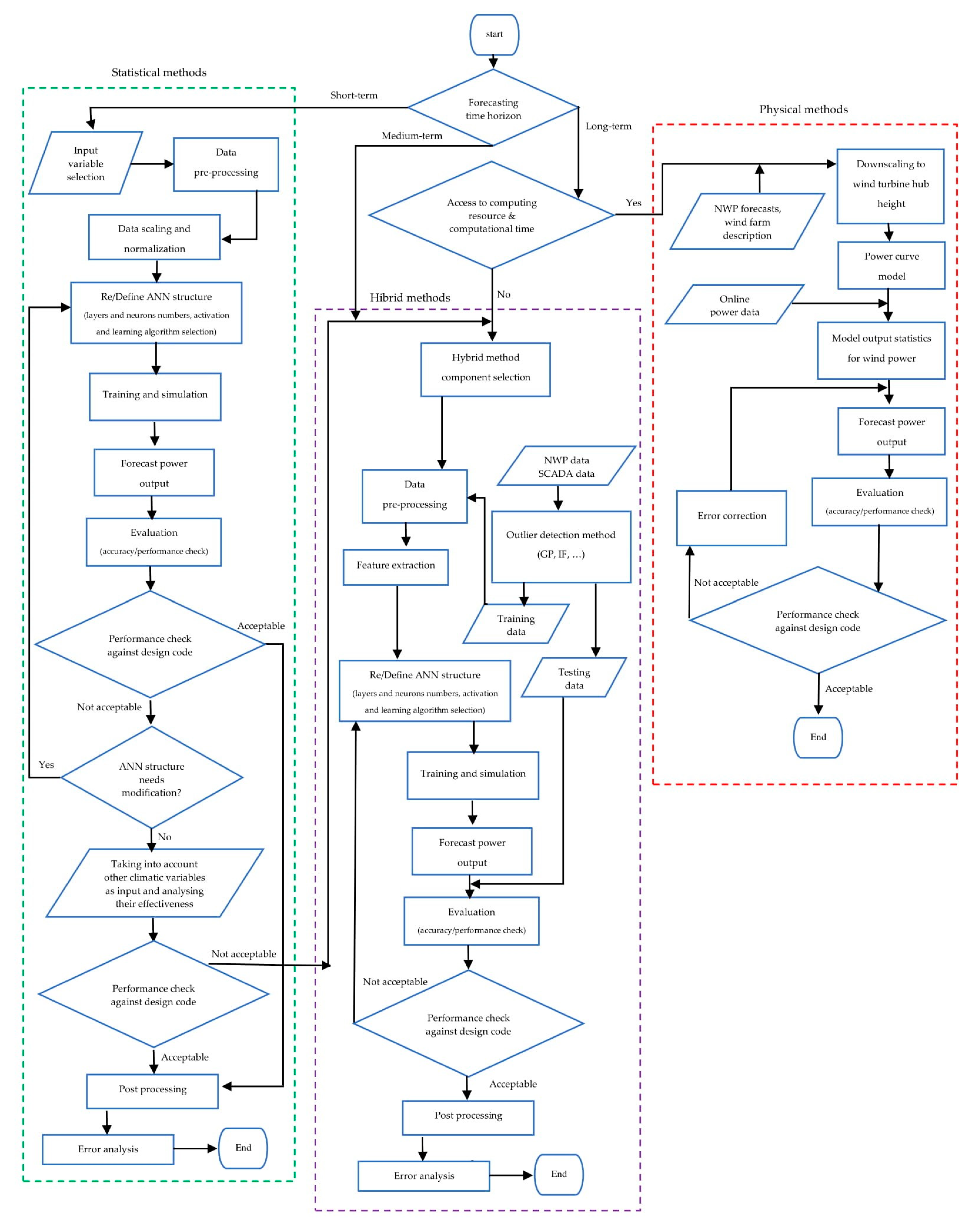
6. Flowchart of Wind Power Forecasting
7. Conclusions
- (1)
- With the continuous development of high-rated wind turbines, power forecasting will keep increasing its significant role in wind turbine operating stages. More advanced and cost-effective prediction methods need to be developed to better forecast generated power from large-scale wind farms. More specifically, new hybrid methods, including incorporating numerical simulations and neural network, and more advanced combination, such as ensemble learning methods, are recommended.
- (2)
- The development of modern computers and storage methods allow handling a larger amount of database. Meanwhile, the larger size of the database has generated new challenges in terms of data preprocessing and error post-processing. Future studies should focus on developing less computational-extensive methods and removing the noise of the raw data.
- (3)
- Future wind farms are gradually moving from onshore sites to offshore ones. Offshore wind turbines, especially floating wind turbines, are operating in a different weather condition and terrain. Future wind power prediction methods should focus on developing appropriate methods for offshore wind prediction, especially the selection of features in coastal and offshore zones to balance between accuracy and efficiency.
- (4)
- To solve wind power forecasting (a typical regression problem), the perfect predictive model will provide zero error, which is the best performance. However, all wind power forecasting models contain errors due to the stochastic nature of wind and therefore, a perfect score does not exist in practice. Many factors can influence the accuracy of a predictive model, such as specific sizes and sampling rates of training/testing/validation datasets, used algorithms and model optimizations. Overall, the performance of predictive models is relative and need to be evaluated through a baseline model. Based on the reviewed literature, most investigators used diverse robust baseline models to compare the performance of their newly developed methods. Nevertheless, a widely accepted baseline method of wind power forecasting has not reached a common view in the current research community. A further investigation is still required in developing a baseline model that works reliably in benchmarking other forecasting methods.
Author Contributions
Funding
Conflicts of Interest
Nomenclature
| Latin symbols | |
| Cp | power coefficient |
| normalised error | |
| mean normalised error | |
| i | hour |
| time horizon | |
| M | total number of predicted data |
| n | number of data points |
| P | wind power |
| p | order of autoregressive |
| measured value of the kth SCADA data point | |
| predicted wind power of the kth data point from deep learning modelling | |
| measured value from the SCADA database | |
| Predicted wind power from deep learning modelling | |
| target measured power | |
| q | order of moving average model |
| R | radius of the rotor |
| forecasted power | |
| u | wind speed |
| forecasted wind power | |
| Greek symbols | |
| φi | autoregressive parameter |
| θj | moving average parameter |
| αt | white noise |
| ρ | air density |
| Abbreviation | |
| ACC | Anomaly Correlation Coefficient |
| ADAM | Adaptive Moment Estimation |
| AE | Average Error |
| DISP | phase error |
| ANFIS | Adaptive Neuro-Fuzzy Inference System |
| ANN | Artificial Neural Network |
| AR | Autoregressive |
| ARX | Autoregressive with exogenous variable |
| ARIMA | Autoregressive Integrated Moving Average |
| ARMA | Autoregressive Moving Average |
| AWNN | Adaptive Wavelet Neural Network |
| BP | Back Propagation |
| BPNN | Back-Propagation Neural Network |
| BRAMS | Brazilian Atmospheric Modelling System |
| CNN | Convolutional Neural Network |
| DBN | Deep Belief Network |
| DGF | Double Gaussian Function |
| ELM | Extreme Learning Machine |
| ENN | Elman Neural Network |
| EVS | Explained Variance Score |
| FFNN | Feed Forward Neural Network |
| GA | Genetic Algorithm |
| GFS | Global Forecasting System |
| GMM | Gaussian Mixture Model |
| GP | Gaussian Process |
| IF | Isolation Forest |
| LSSVM | Least Square Support Vector Machine |
| LSTM | Long Short-Term Memory |
| MA | Moving Average |
| MAE | Mean Absolute Error |
| MAPE | Mean Absolute Percentage Error |
| MARE | Mean Absolute Relative Error |
| MDN | Mixture Density Neural Network |
| MFNN | Multilayer Feedforward Neural Network |
| MLP | Multilayer Perceptron |
| MODA | Multi-Objective Dragonfly Algorithm |
| MSE | Mean Square Error |
| MSLE | Mean Squared Logarithmic Error |
| NAAE | Normalised Absolute Average Error |
| NMAE | Normalised Mean Absolute Error |
| NMBE | Normalized Mean Bias Error |
| NMSE | Normalized Mean Square Error |
| NN | Neural Network |
| NRMSE | Normalised Root Mean Square Error |
| NSC | Nash–Sutcliffe Coefficient |
| NWP | Numerical Weather Prediction |
| PCC | Pearson Correlation Coefficient |
| PSO | Particle Swarm Optimisation |
| R2 | R-Square |
| RBFNN | Radial Basis Function Neural Network |
| RMSE | Root Mean Square Error |
| RVM | Relative Vector Machine |
| SCADA | Supervisory Control and Data Acquisition |
| SDE | Standard Deviation Error |
| SNMAE | Square Normalized Mean Bias Error |
| TWh | Terawatt-hour |
| WECS | Wind Energy Conversion System |
| WNN | Wavelet Neural Network |
References
- Bilal, B.; Ndongo, M.; Adjallah, K.H.; Sava, A.; Kebe, C.M.F.; Ndiaye, P.A.; Sambou, V. Wind turbine power output prediction model design based on artificial neural networks and climatic spatiotemporal data. In Proceedings of the IEEE International Conference on Industrial Technology 2018, Lyon, France, 20–22 February 2018; pp. 1085–1092. [Google Scholar]
- Gielen, D.; Boshell, F.; Saygin, D.; Bazilian, M.D.; Wagner, N.; Gorini, R. The role of renewable energy in the global energy transformation. Energy Strategy Rev. 2019, 24, 38–50. [Google Scholar] [CrossRef]
- Lin, Z.; Liu, X. Assessment of wind turbine aero-hydro-servo-elastic modelling on the effects of mooring line tension via deep learning. Energies 2020, 13, 2264. [Google Scholar] [CrossRef]
- Zhang, J.; Yan, J.; Infield, D.; Liu, Y.; Lien, F. sang Short-term forecasting and uncertainty analysis of wind turbine power based on long short-term memory network and Gaussian mixture model. Appl. Energy 2019, 241, 229–244. [Google Scholar] [CrossRef] [Green Version]
- Zhao, Y.; Ye, L.; Li, Z.; Song, X.; Lang, Y.; Su, J. A novel bidirectional mechanism based on time series model for wind power forecasting. Appl. Energy 2016, 177, 793–803. [Google Scholar] [CrossRef]
- Wang, X.; Guo, P.; Huang, X. Energy Procedia A Review of Wind Power Forecasting Models. Energy Procedia 2011, 12, 770–778. [Google Scholar] [CrossRef] [Green Version]
- Renewable Electricity Capacity and Generation. Available online: https://assets.publishing.service.gov.uk/government/uploads/system/uploads/attachment_data/file/875410/Renewables_Q4_2019.pdf (accessed on 26 March 2020).
- Singh, S.; Bhatti, T.S.; Kothari, D.P. Wind power estimation using artificial neural network. J. Energy Eng. 2007, 133, 46–52. [Google Scholar] [CrossRef]
- Sharma, R.; Singh, D. A Review of Wind Power and Wind Speed Forecasting. Rahul Sharma J. Eng. Res. and Appl. 2018, 8, 1–9. [Google Scholar]
- Wu, Y.; Hong, J. A literature review of wind forecasting technology in the world. In Proceedings of the IEEE Lausanne Power Tech, Lausanne, Switzerland, 1–5 July 2007; pp. 504–509. [Google Scholar]
- Soman, S.S.; Zareipour, H.; Malik, O.; Mandal, P. A review of wind power and wind speed forecasting methods with different time horizons. In Proceedings of the 2010 North American Power Symposium (NAPS 2010), Arlington, TX, USA, 26–28 September 2010; pp. 1–8. [Google Scholar]
- Jung, J.; Broadwater, R.P. Current status and future advances for wind speed and power forecasting. Renew. Sustain. Energy Rev. 2014, 31, 762–777. [Google Scholar] [CrossRef]
- Chang, W.-Y. A Literature Review of Wind Forecasting Methods. J. Power Energy Eng. 2014, 2, 161–168. [Google Scholar] [CrossRef]
- De Felice, M.; Alessandri, A.; Ruti, P.M. Electricity demand forecasting over Italy: Potential benefits using numerical weather prediction models. Electr. Power Syst. Res. 2013, 104, 71–79. [Google Scholar] [CrossRef]
- De Giorgi, M.G.; Ficarella, A.; Tarantino, M. Assessment of the benefits of numerical weather predictions in wind power forecasting based on statistical methods. Energy 2011, 36, 3968–3978. [Google Scholar] [CrossRef]
- Focken, U.; Lange, M.; Waldl, H.-P.H.-P. Previento-A Wind Power Prediction System with an Innovative Upscaling Algorithm. In Proceedings of the European Wind Energy Conference (EWEC), Copenhagen, Denmark, 2–6 July 2001; pp. 1–4. [Google Scholar]
- Foley, A.M.; Leahy, P.G.; Marvuglia, A.; McKeogh, E.J. Current methods and advances in forecasting of wind power generation. Renew. Energy 2012, 37, 1–8. [Google Scholar] [CrossRef] [Green Version]
- Jung, S.; Kwon, S.D. Weighted error functions in artificial neural networks for improved wind energy potential estimation. Appl. Energy 2013, 111, 778–790. [Google Scholar] [CrossRef]
- Durán, M.J.; Cros, D.; Riquelme, J. Short-term wind power forecast based on ARX models. J. Energy Eng. 2007, 133, 172–180. [Google Scholar] [CrossRef]
- Gallego, C.; Pinson, P.; Madsen, H.; Costa, A.; Cuerva, A. Influence of local wind speed and direction on wind power dynamics-Application to offshore very short-term forecasting. Appl. Energy 2011, 88, 4087–4096. [Google Scholar] [CrossRef] [Green Version]
- Firat, U.; Engin, S.N.; Sarcalar, M.; Ertuzum, A.B. Wind Speed Forecasting Based on Second Order Blind Identification and Autoregressive Model. In Proceedings of the 2010 Ninth International Conference on Machine Learning and Applications, Washington, DC, USA, 12–14 December 2010; pp. 686–691. [Google Scholar]
- Wu, Y.R.; Zhao, H.S. Optimization maintenance of wind turbines using Markov decision processes. In Proceedings of the 2010 International Conference on Power System Technology: Technological Innovations Making Power Grid Smarter, POWERCON2010, Hangzhou, China, 24–28 October 2010; pp. 1–6. [Google Scholar]
- Lin, Z.; Liu, X. Wind power forecasting of an offshore wind turbine based on high-frequency SCADA data and deep learning neural network. Energy 2020, 201, 117693. [Google Scholar] [CrossRef]
- Lee, K.; Booth, D.; Alam, P. A comparison of supervised and unsupervised neural networks in predicting bankruptcy of Korean firms. Expert Syst. Appl. 2005, 29, 1–16. [Google Scholar] [CrossRef]
- Marugán, A.P.; Márquez, F.P.G.; Perez, J.M.P.; Ruiz-Hernández, D. A survey of artificial neural network in wind energy systems. Appl. Energy 2018, 228, 1822–1836. [Google Scholar] [CrossRef] [Green Version]
- Wang, J.; Yang, W.; Du, P.; Niu, T. A novel hybrid forecasting system of wind speed based on a newly developed multi-objective sine cosine algorithm. Energy Convers. Manag. 2018, 163, 134–150. [Google Scholar] [CrossRef]
- Sideratos, G.; Hatziargyriou, N.D. Probabilistic Wind Power Forecasting Using Radial Basis Function Neural Networks. IEEE Trans. Power Syst. 2012, 27, 1788–1796. [Google Scholar] [CrossRef]
- Hong, Y.Y.; Rioflorido, C.L.P.P. A hybrid deep learning-based neural network for 24-h ahead wind power forecasting. Appl. Energy 2019, 250, 530–539. [Google Scholar] [CrossRef]
- Pelletier, F.; Masson, C.; Tahan, A. Wind turbine power curve modelling using artificial neural network. Renew. Energy 2016, 89, 207–214. [Google Scholar] [CrossRef]
- Sideratos, G.; Hatziargyriou, N.D. An advanced statistical method for wind power forecasting. IEEE Trans. Power Syst. 2007, 22, 258–265. [Google Scholar] [CrossRef]
- Jyothi, M.N.; Rao, P.V.R. Very-short term wind power forecasting through Adaptive wavelet neural network. In Proceedings of the 2016-Biennial International Conference on Power and Energy Systems: Towards Sustainable Energy, PESTSE 2016, Bengaluru, India, 21–23 January 2016; IEEE: Piscataway, NJ, USA. [Google Scholar]
- Xu, L.; Mao, J. Short-term wind power forecasting based on Elman neural network with particle swarm optimization. In Proceedings of the 28th Chinese Control and Decision Conference, CCDC 2016, Yinchuan, China, 28–30 May 2016; pp. 2678–2681. [Google Scholar]
- Catalão, J.P.S.; Pousinho, H.M.I.; Member, S.; Mendes, V.M.F. An Artificial Neural Network Approach for Short-Term Wind Power Forecasting in Portugal. In Proceedings of the 2009 15th International Conference on Intelligent System Applications to Power Systems (ISAP 2009), Curitiba, Brazil, 8–12 November 2009; pp. 1–5. [Google Scholar]
- Chang, W. Application of Back Propagation Neural Network for Wind Power Generation Forecasting. Int. J. Digit. Content Technol. Appl. 2013, 7, 502–509. [Google Scholar]
- Carolin Mabel, M.; Fernandez, E. Analysis of wind power generation and prediction using ANN: A case study. Renew. Energy 2008, 33, 986–992. [Google Scholar] [CrossRef]
- Lin, Z.; Liu, X.; Collu, M. Wind power prediction based on high-frequency SCADA data along with isolation forest and deep learning neural networks. Int. J. Electr. Power Energy Syst. 2020, 118, 105835. [Google Scholar] [CrossRef]
- Marcos, J.; Alexandre, L.; Saulo, K.G.; Jairo, R.F.; Mattos, J.G.Z. De A Meteorological–Statistic Model for Short-Term Wind Power Forecasting. J. Control Autom. Electr. Syst. 2017, 28, 679–691. [Google Scholar]
- Wang, J.; Yang, W.; Du, P.; Li, Y. Research and application of a hybrid forecasting framework based on multi-objective optimization for electrical power system. Energy 2018, 148, 59–78. [Google Scholar] [CrossRef]
- Shetty, R.P.; Sathyabhama, A.; Srinivasa, P.P.; Adarsh Rai, A. Optimized radial basis function neural network model for wind power prediction. In Proceedings of the 2016 Second International Conference on Cognitive Computing and Information Processing (CCIP 2016), Mysuru, India, 12–13 August 2016; Institute of Electrical and Electronics Engineers Inc.: Piscataway, NJ, USA. [Google Scholar]
- Liu, J.; Wang, X.; Lu, Y. A novel hybrid methodology for short-term wind power forecasting based on adaptive neuro-fuzzy inference system. Renew. Energy 2017, 103, 620–629. [Google Scholar] [CrossRef]
- Zhao, P.; Wang, J.; Xia, J.; Dai, Y.; Sheng, Y.; Yue, J. Performance evaluation and accuracy enhancement of a day-ahead wind power forecasting system in China. Renew. Energy 2012, 43, 234–241. [Google Scholar] [CrossRef]
- Kou, P.; Gao, F.; Guan, X. Sparse online warped Gaussian process for wind power probabilistic forecasting. Appl. Energy 2013, 108, 410–428. [Google Scholar] [CrossRef]
- Giorgi, M.G.D.; Congedo, P.M.; Malvoni, M.; Laforgia, D. Error analysis of hybrid photovoltaic power forecasting models: A case study of mediterranean climate. Energy Convers. Manag. 2015, 100, 117–130. [Google Scholar] [CrossRef]
- Louka, P.; Galanis, G.; Siebert, N.; Kariniotakis, G.; Katsafados, P.; Pytharoulis, I.; Kallos, G. Improvements in wind speed forecasts for wind power prediction purposes using Kalman filtering. J. Wind Eng. Ind. Aerodyn. 2008, 96, 2348–2362. [Google Scholar] [CrossRef] [Green Version]
- Ziegler, L.; Gonzalez, E.; Rubert, T.; Smolka, U.; Melero, J.J. Lifetime extension of onshore wind turbines: A review covering Germany, Spain, Denmark, and the UK. Renew. Sustain. Energy Rev. 2018, 82, 1261–1271. [Google Scholar] [CrossRef] [Green Version]
- Yang, W.; Court, R.; Jiang, J. Wind turbine condition monitoring by the approach of SCADA data analysis. Renew. Energy 2013, 53, 365–376. [Google Scholar] [CrossRef]
- Manobel, B.; Sehnke, F.; Lazzús, J.A.; Salfate, I.; Felder, M.; Montecinos, S. Wind turbine power curve modeling based on Gaussian Processes and Artificial Neural Networks. Renew. Energy 2018, 125, 1015–1020. [Google Scholar] [CrossRef]
- Vaccaro, A.; Mercogliano, P.; Schiano, P.; Villacci, D. An adaptive framework based on multi-model data fusion for one-day-ahead wind power forecasting. Electr. Power Syst. Res. 2011, 81, 775–782. [Google Scholar] [CrossRef]
- Peng, H.; Liu, F.; Yang, X. A hybrid strategy of short term wind power prediction. Renew. Energy 2013, 50, 590–595. [Google Scholar] [CrossRef]
- Lange, M.; Focken, U. New developments in wind energy forecasting. In Proceedings of the IEEE Power and Energy Society 2008 General Meeting: Conversion and Delivery of Electrical Energy in the 21st Century, PES 2008, Pittsburgh, PA, USA, 20–24 July 2008; pp. 1–8. [Google Scholar]
- Lydia, M.; Kumar, S.S.; Selvakumar, A.I.; Prem Kumar, G.E. A comprehensive review on wind turbine power curve modeling techniques. Renew. Sustain. Energy Rev. 2014, 30, 452–460. [Google Scholar] [CrossRef]
- Lange, B.; Rohrig, K.; Ernst, B.; Schlögl, F.; Cali, Ü.; Jursa, R.; Moradi, J. Probabilistic Forecasts for Daily Power Production. In Proceedings of the Eurepean Wind Energy Conference, Athens, Greece, 27 February–2 March 2006. [Google Scholar]
- Velázquez, S.; Carta, J.A.; Matías, J.M. Influence of the input layer signals of ANNs on wind power estimation for a target site: A case study. Renew. Sustain. Energy Rev. 2011, 15, 1556–1566. [Google Scholar] [CrossRef]
- Al-Yahyai, S.; Charabi, Y.; Al-Badi, A.; Gastli, A. Nested ensemble NWP approach for wind energy assessment. Renew. Energy 2012, 37, 150–160. [Google Scholar] [CrossRef]


| Time Horizon | Range | Applications |
|---|---|---|
| very short-term | few minutes to 30 min | regulation actions, real-time grid operations, market clearing, turbine control |
| short-term | 30 min to 6 h | load dispatch planning, load intelligent decisions |
| medium-term | 6 h to 1 day | operational security in the electricity market, energy trading, on-line and off-line generating decisions |
| long-term | 1 day to a month | reserve requirements, maintenance schedules, optimum operating cost, operation management |
| References | Method | Input Features | Datasets | Data Size | Sampling Rate |
|---|---|---|---|---|---|
| M. Duran et al. 2007 [19] | ARX | wind speed | Spanish wind farms | 12 months | 6 h |
| Gallego et al., 2011 [20] | AR model | wind speed, wind direction | offshore 160 MW wind farm of Horns Rev in Denmark | 12 months | 10 min |
| References | Algorithm | Input Features | Datasets | Data Size | Sampling Rate |
|---|---|---|---|---|---|
| Pelletier et al., 2016 [29] | MLP | wind speed, air density, turbulence intensity, wind shear, wind direction and yaw error | 140 wind turbines in Nordic | 12 months | 10 min |
| Sideratos et al., 2007 [30] | RBFNN | past power measurements, NWPs (wind speed and direction) | offshore wind farm in Denmark including 35 600-KW turbines | 26 months | 1 min |
| Bilal et al., 2018 [1] | MLP | wind speed | four sites on the northwest coast of Senegal. | 6~9 months | 1 and 10 min |
| Jyothi and Rao, 2016 [31] | Adaptive wavelet NN (AWNN) | wind speed, air density, ambient temperature, and wind direction | two wind turbines in North India | 15 days | 10 min |
| Zhao et al., 2016 [5] | Bidirectional ELM | wind power | onshore wind farm in the USA | 12 months | 60 min |
| De Giorgi et al., 2011 [15] | ENN | wind power, wind speed, pressure temperature and relative humidity | wind farm in southern Italy | 12 months | 60 min |
| Xu and Mao, 2016 [32] | ENN | wind speed, wind direction, temperature, humidity, pressure | a single 15 kW wind turbine in a west wind farm in China | 6 days | 15 min |
| Catalao et al., 2009 [33] | MFNN (trained by LM algorithm) | historical data | wind farm in Portugal | 4 days | |
| Singh et al. 2007 [8] | MLP | wind speed, wind direction and air density | Fort Davis Wind Farm the in Texas, USA | 2 months | 10 min |
| Chang, 2013 [34] | BPNN | wind power | a wind turbine installed in Taichung coast of Taiwan | 6 days | 10 min |
| Carolin and Fernandez, 2008 [35] | Feed-forward NN (MLP) | wind speed, relative humidity, and generation hour | 137 wind turbines from seven wind farms located in Muppandal, (India) | 36 months |
| References | Method | Input Features | Datasets | Data Size | Sampling Rate |
|---|---|---|---|---|---|
| Hong et al. 2019 [28] | CNN, RBFNN, DGF | wind power | historical power data of a wind farm in Taiwan | 12 months | 60 min |
| Lin et al., 2020 [36] | Isolation Forest (IF), deep learning NN | wind speed, nacelle orientation, yaw error, blade pitch angle, and ambient temperature | SCADA data of a wind turbine in Scotland | 12 months | 1 s |
| Zhang et al., 2019 [4] | LSTM, Gaussian Mixture Model (GMM) | wind speed | a wind farm of 123 units in north China | 3 months | 15 min |
| Marcos et al. 2017 [37] | Kalman filter, statistical regression or power curve | NWP data | Palmas and RN05 wind farms in Brazil | 7 and 12 months | 10 min |
| Wang et al., 2018 [38] | ELM optimised by MODA | wind speed | two observation sites in Penglai, China | 37 days | 10 min |
| Shetty et al., 2016 [39] | RBFNN, PSO in optimising and ELM in training | wind speed, wind direction, blade pitch angle, density, rotor speed | SCADA of a 1.5 MW horizontal wind turbine | 6 months | 10 min |
| De Giorgi et al., 2011 [15] | Elman and MLP network | wind power, wind speed, pressure, temperature, humidity | wind farm in southern Italy | 12 months | 60 min |
| De Giorgi et al., 2011 [15] | Wavelet decomposition and Elman network | wind power, wind speed, pressure, temperature and relative humidity | wind farm in southern Italy | 12 months | 60 min |
| Liu et al., 2017 [40] | BPNN, RBFNN and LSSVM | wind speed, wind direction, and temperature at the wind turbine hub height | 16 MW wind farm located in Sichuan, China | 2 months | 15 min |
| Zhao et al., 2012 [41] | Kalman filter and MFNN | wind speed, direction, temperature, pressure, humidity power data from SCADA | an outermost domain which covers the eastern half of China | 12 months | 6 h |
| Lin and Liu 2020 [36] | IF feed-forward NN | wind speed, blade pitch angle, temperature, yaw error and nacelle orientation | 7 MW wind turbine in Scotland owned by the ORE Catapult | 12 months | 1 s |
| Peng et al., 2013 [42] | Physical model and ANN | wind speed, wind direction, temperature | 50 MW wind farm with 40 wind turbines in China | 3 months | 10 min |
| References | Algorithm | Evaluation Criteria | Evaluation Value | Evaluation Unit | Results |
|---|---|---|---|---|---|
| Duran et al., 2007 [19] | ARX | ME | 34.6–63.2 | Accuracy improvement was found in comparison with the persistence method and conventional AR models. | |
| Gallego et al., 2011 [20] | AR | NRMSE | 3.93 | Local measurement of both wind speed and direction improves the forecasting performance. |
| References | Algorithm | Evaluation Criteria | Evaluation Value | Evaluation Unit | Results |
|---|---|---|---|---|---|
| Pelletier et al., 2016 [29] | MLP | MAE | 15.3–15.9 | kW | Multi-stage ANN with 6 inputs performed better than parametric, non-parametric and discrete models. |
| Sideratos et al., 2007 [30] | RBFNN | NMAE | 5–14 | % | Effectively predicted for 1-48 h ahead performed better than the persistence method. |
| NRMSE | 20 | % | |||
| Bilal et al., 2018 [1] | MLP | NMSE | 3.51 | % | Wind speed + temperature as input is better than only wind speed. Considering all variables improves performance. |
| NMAE | 14.85 | % | |||
| SNMAE | 25.7 | ||||
| R (fitting rate) | 0.98 | % | |||
| Jyothi and Rao, 2016 [31] | AWNN | NRMSE | 0.1647 | The minimum NRMSE showed that WNN performs well. | |
| Zhao et al., 2016 [5] | Bidirectional ELM | NMBE | −0.53 | % | Lower values of NMAE and NRMSE showed that bidirectional performed better than forward, backward and persistence method. |
| NMAE | 16.61 | % | |||
| NRMSE | 21.27 | % | |||
| De Giorgi et al., 2011 [15] | ENN | NAAE | 15 | % | Among the different NWPs data, pressure, and temperature had the highest positive impact. The hybrid method performed better than other methods especially in long term forecast (24 h). |
| 12.5 | % | ||||
| Xu and Mao, 2016 [32] | ENN | MSE | 16.55 | % | Application of particle swarm optimisation algorithm improves the performance/accuracy. |
| MAE | 10.52 | % | |||
| Catalao et al., 2009 [33] | MFNN (trained by LM algorithm) | MAPE | 7.26 | % | Performed better than the persistence method in less than 5 s of computing time. |
| Singh et al., 2007 [8] | MLP | Percentage difference | 0.303–1.082 | % | Better results than traditional methods. |
| Chang, 2013 [34] | BPNN | AAE | 0.278 | % | The proposed model can predict wind power easily and correctly. |
| Carolin and Fernandez, 2008 [35] | feed forward NN (MLP) | RMSE | 8.06 | % | Helpful model for energy planners. |
| References | Method | Evaluation Criteria | Evaluation Value | Evaluation Unit | Results |
|---|---|---|---|---|---|
| Hong et al., 2019 [28] | CNN, RBFNN, DGF | R2 | 0.92 | Best performance rather than CNN-RBFNN and CNN-MFNN (lower RMSE, NMSE, MAPE and higher R2). | |
| RMSE | 76.97 | % | |||
| NMSE | 2.75 | % | |||
| MAPE | 5.048 | % | |||
| Lin et al., 2020 [36] | IF, deep learning NN | MSE | 0.003 | Using IF for outlier detection instead of Elliptic envelope increased the performance. | |
| Zhang et al., 2019 [4] | LSTM, GMM | RMSE | 6.37 | % | The accuracy of LSTM was higher than RBF, wavelet, DBN, BP and ELMAN.GMM was better in analysing the uncertainty of the prediction than MDN and RVM. |
| Marcos et al., 2017 [37] | Kalman filter, statistical regression or power curve | MBE | 4.32 | kW | Using Kalman filter decreased the RMSE and increased the ACC and NSC, all represent better forecasting. |
| RMSE | 101.11 | ||||
| Wang et al., 2018 [38] | ELM optimised by MODA | AE | 19.05 | MW | |
| MAE | 77.67 | MW | |||
| RMSE | 107.96 | MW | |||
| NMSE | 0.0001 | ||||
| MAPE | 0.9824 | % | |||
| Shetty et al., 2016 [39] | RBFNN, PSO in optimising and ELM in training | MSE | 0.0003 | ELM as a learning algorithm makes the learning process quicker. | |
| De Giorgi et al., 2011 [15] | Elman and MLP network based on historical data and NWP | NAAE | 10.98 | % | Among the different NWPs data, pressure and temperature had the highest positive impact. The hybrid method performed better than other methods especially in long term forecast (24 h). |
| De Giorgi et al., 2011 [15] | Wavelet decomposition and Elman network | NAAE | 15.5 | % | |
| Liu et al., 2017 [40] | BPNN, RBFNN and LSSVM | MAPE | 6.7–27.4 | % | The combined model performed better than all three individual models |
| NMAE | 1.01–6.35 | % | |||
| NRMSE | 2.37–9.45 | % | |||
| Zhao et al., 2012 [41] | Kalman filter, MFNN | NRMSE | 16.47 | % | NRMSE value improved from 17.81% to 16.47%, by using a Kalman filter. |
| Lin and Liu, 2020 [36] | IF, feed-forward neural network | RMSE | 517.33 | Blade pitch angle had the greatest effect on the performance of the prediction model even more than wind speed and wind shear. | |
| MAE | 374.41 | ||||
| R-square | 0.91 | ||||
| MSLE | 0.29 | ||||
| EVS | 0.91 | ||||
| Peng et al., 2013 [42] | Physical + ANN | MAE | 760 | kW | Combining physical and statistical prediction techniques rather than the application of ANN improved accuracy. |
| RMSE | 2.01 | % |
© 2020 by the authors. Licensee MDPI, Basel, Switzerland. This article is an open access article distributed under the terms and conditions of the Creative Commons Attribution (CC BY) license (http://creativecommons.org/licenses/by/4.0/).
Share and Cite
Hanifi, S.; Liu, X.; Lin, Z.; Lotfian, S. A Critical Review of Wind Power Forecasting Methods—Past, Present and Future. Energies 2020, 13, 3764. https://doi.org/10.3390/en13153764
Hanifi S, Liu X, Lin Z, Lotfian S. A Critical Review of Wind Power Forecasting Methods—Past, Present and Future. Energies. 2020; 13(15):3764. https://doi.org/10.3390/en13153764
Chicago/Turabian StyleHanifi, Shahram, Xiaolei Liu, Zi Lin, and Saeid Lotfian. 2020. "A Critical Review of Wind Power Forecasting Methods—Past, Present and Future" Energies 13, no. 15: 3764. https://doi.org/10.3390/en13153764