Article

Adjusting the Single-Diode Model Parameters of a Photovoltaic Module with Irradiance and Temperature

1
School of Engineering, University of Wolverhampton, Telford TF2 9NT, UK
2
Department of Electrical Technique, Southern Technical University, Technical Institute-Qurna, Basra, Iraq
*
Author to whom correspondence should be addressed.
Energies 2020, 13(12), 3226; https://doi.org/10.3390/en13123226
Submission received: 30 May 2020 / Revised: 16 June 2020 / Accepted: 17 June 2020 / Published: 22 June 2020
(This article belongs to the Special Issue Solar Photovoltaics and Solar Thermal Energy Systems)

Abstract

:
This paper presents a concise discussion and an investigation of the most literature-reported methods for modifying the lumped-circuit parameters of the single-diode model (SDM) of a photovoltaic (PV) module, to suit the prevailing climatic conditions of irradiance and temperature. These parameters provide the designer of a PV system with an essential design and simulation tool to maximize the efficiency of the system. The parameter modification methods were tested using three commercially available PV modules of different PV technologies, namely monocrystalline, multicrystalline, and thin film types. The SDM parameters of the three test modules were extracted under standard test conditions (STC) using a well-established numerical technique. Using these STC parameters as reference values, the parameter adjustment methods were subsequently deployed to calculate the modified parameters of the SDM under various operating conditions of temperature and irradiance using MATLAB-based software. The accuracy and effectiveness of these methods were evaluated by a comparison between the calculated and measured values of the modified parameters.

Graphical Abstract

1. Introduction

Photovoltaic systems offer the most direct conversion of the electromagnetic energy in the sunlight into electricity. At the heart of any PV power plant is the PV generator, which typically consists of an array of PV modules connected in series-parallel combinations to deliver the rated power at the required levels of terminal current and voltage. Each PV module consists of several PV cells, which are almost always connected in series to provide a specific terminal voltage. The terminal I-V (current-voltage) and P-V (power-voltage) characteristics of a typical PV generator, whether it is a cell, a module, or an array, are shown in Figure 1. Three salient points can be identified on the I-V curve: The short circuit (SC), the open circuit (OC), and the maximum power point (MPP).
The design of a PV power system requires a lumped-circuit parameters’ model of the PV generator. This is used for purposes, such as to properly size the power switching devices used in the power processing converters, designing the maximum power point tracking system, and for efficient sizing of the PV array. In addition, such an equivalent circuit model can be readily embedded in circuit simulation programs. The widely accepted circuit model of a PV generator is the single-diode model (SDM), which is also included in Figure 1 [1,2,3]. This model can be easily adapted to model a cell, a module, or an array and offers a compromise between accuracy and complexity [4,5,6]. An extensive study on the measurement uncertainty using different lumped-circuit parameters models of a PV module can be found in [7]. However, this paper was based on the single-diode model.
The SDM involves five parameters: The photocurrent I p h , the saturation current I s a t , and the ideality factor n of the diode, the parallel resistance R s h , and the series resistance R s . These parameters are not provided in manufacturers’ datasheets of PV modules. However, they can be extracted from data given in a datasheet, which almost always includes the three salient points (SC, OC, and MPP), the number of series-connected cells N S , and the temperature coefficients of the short-circuit current μ I S C   ( A / ) and open-circuit voltage μ V O C ( V / ) [8]. However, these parameters are always specified at only one operating condition, namely the STC (STC: Irradiance G = 1000   ( W . m 2 ) , air mass ratio AM = 1.5, and temperature T = 25   ) . Since the characteristics of a PV generator can vary significantly with the ambient temperature and irradiance, parameters estimated from information in a datasheet are only valid at standard test conditions. For any other arbitrary values of temperature and irradiance, these parameters must be adjusted, i.e., re-estimated, accordingly [9,10]. It is worth noting at this point that the problem of variations in module parameters is further complicated due to the effects of partial shading (PS) [11,12], which can have adverse consequences on the performance and energy yield of a PV plant. Alleviation of the effects of PS requires the use of bypass diodes. However, these diodes can vary the parameters of the PV generator and also give rise to complicated P-V curves with multiple power peaks [13,14]. However, the focus of this paper was on exploring the performance of methods for varying the parameters of the SDM with variations in irradiance and temperature without including the effects of bypass diodes.
Two different approaches have been reported in the literature for considering the variations of the SDM parameters with fluctuations in ambient climatic conditions [15]. The first approach assumes that the photocurrent depends only on irradiance, while the saturation current depends only on temperature, while all other parameters remain constant [16,17]. The second approach assumes that the saturation current and the resistances vary with both conditions of irradiance and temperature [18]. The ideality factor is, however, assumed to remain constant in both approaches. The contributions of this paper are: Review the major methods of modifying the parameters of the SDM with due account taken of their variations with temperature and irradiance, provide the mathematical derivation of these methods, which is not generally provided in the literature, apply these methods to PV modules of different technologies, and compare their results.
Following this introduction, Section 2 presents the mathematical background that underpins the rest of the work discussed in this paper. The most reported methods of modifying the STC parameters of the SDM according to changes in irradiance and temperature, referred to henceforth as the parameter adjustment methods, are presented and discussed in Section 3. Section 4 presents the outcome of synthesizing the results of these adjustment methods when applied to three PV modules of different PV technologies and compares these results with measured values. Finally, Section 5 summarizes the outcomes of this article.

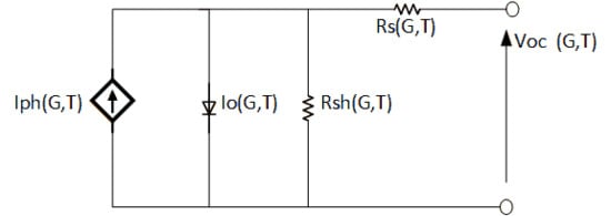
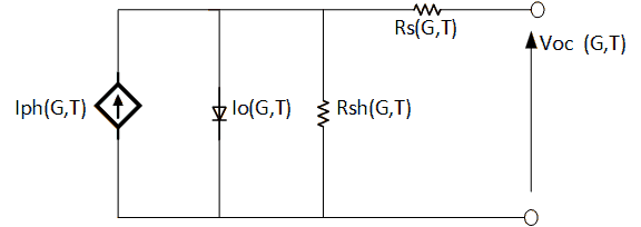
2. Mathematical Analysis of the Single-Diode Model

This section presents the mathematical analyses of the single-diode model that pertains to the parameter adjustment methods, which are the subject of the next section.
A PV module with N S series-connected PV cells can be modelled using the SDM depicted in Figure 1. The terminal current I (A) and voltage V (V) of the module are expressed by the nonlinear, implicit, and transcendental equation:
I = I p h I s a t [ exp ( V + I R s n N s V t h ) 1 ] V + I R s R s h
Referring to Figure 1, the current I p h represents the photocurrent, which is mainly dependent on the incident irradiance G [19]. The second term is the diode current I d , which is represented by Shockley’s equation, and the last term is the current I s h , which flows in the parallel resistance R s h . Finally, V t h ( V ) is the thermal equivalent voltage, which is given in terms of the electronic charge q = 1.602 × 10 19   C , the temperature T ( K ) , and Boltzmann’s constant k = 1.3806503 × 10 23   J / K as:
V t h = k T / q .
Substituting ( V o c   , 0 ) in Equation (1), we obtain the open-circuit equation:
OC :              I p h    = I s a t [ exp ( V o c n N s V t h ) 1 ] + V o c R s h .
Since V o c n N s V t h   1 , the (−1) in the exponential term can be neglected [20]. Hence, re-arranging, we can express the open-circuit voltage as:
V o c = n N s V t h ln ( I p h R s h V o c I s a t R s h ) .
Substituting ( 0 , I s c   ) in Equation (1), we obtain the short-circuit equation:
SC :           I s c = I p h I s a t [ exp ( I s c R s n N s V t h ) 1 ] I s c R s R s h .
Finally, substituting the MPP point ( V m p , I m p ) into Equation (1), we obtain the MPP equation:
MPP :       I m p = I p h I s a t [ exp ( V m p + I m p R s n N s V t h ) 1 ] V m p + I m p R s R s h .
The derivative d I / d V   is obtained from Equation (1) as:
d I d V = ( I s a t n N s V t h [ exp ( V + I R s n N s V t h ) ] + 1 R s h ) ( ( 1 + R s R s h + I s a t R s n N s V t h exp ( V + I R s n N s V t h ) ) .
This expression for the derivative is valid at any point along the I-V curve of a PV module. The power derivative d P / d V at any point along the P-V curve is:
d P d V = d d V ( V I ) = V I V + I V V .
At the MPP, the derivative d P / d I is equal to zero, thus:
d P d V | MPP = 0 = V m p I V + I m p .
Consequently, at the MPP, we can write:
d I d V | MPP = I m p V m p .
Therefore, at the MPP, from Equations (7) and (10), we can write:
d P d V | MPP = I m V m = 1 R s h I s a t n   N S   V t h e x p ( V m + I m R s n   N s V T ) 1 + R s R s h + I s a t R s n   N S   V t h e x p ( V m + I m R s n   N s V T )   .
The effect of the shunt resistance is dominant at high currents and low voltages, i.e., near the short-circuit point on the I-V curve, hence we may write [17,21]:
d I d V | I s c = 1 R s h   .
The above expressions are the key equations which are used in formulating a variety of analytical [8,22], numerical, and iterative methods [3] for extracting the five parameters of the SDM model and also for formulating the parameter adjustment methods for modifying the SDM parameters according to variations in operating conditions of irradiance and temperature [19,23,24]. In addition to conventional analytical and numerical methods of parameters’ extraction, there are other schemes, such as those based on the meta-heuristic firefly algorithm [25] and those based on computational intelligence, such as [26].

3. Method of Adjusting the SDM Model Parameters

The parameters of the SDM model of a PV module are almost always extracted at standard test conditions. Consequently, these parameters are valid only at STC. But, since the characteristics of a PV module and its model parameters vary considerably with irradiance and temperature, these extracted parameters must be adjusted to match the prevailing environmental conditions of irradiance and ambient temperature [3,9,10].

3.1. Short-Circuit Current

There are two primary methods which express changes of the short-circuit current with irradiance G   and temperature T as described next.

3.1.1. Method 1

In this mostly reported method, the short-circuit current I s c ( G , T ) as a function of irradiance and temperature is given as [15,22,27,28]:
I s c ( G , T ) = G G S T C [ I S C , S T C   + μ I s c ( T T S T C ) ]
where μ I s c ( A / ) is the short-circuit current temperature coefficient, which is always available in a datasheet of a PV module. If dependence on irradiance is neglected:
I s c ( T ) = [ I S C , S T C   + μ I s c ( T T S T C ) ] .
Similarly, if dependence on temperature is ignored:
I s c ( G ) = G G S T C I S C , S T C .

3.1.2. Method 2

This method improves the accuracy of Equation (13) by introducing an exponent to take into account the nonlinear effects of irradiance on the module’s short-circuit current as [23,29,30]:
I s c ( G , T ) = ( G G S T C ) α [ I S C , S T C   + μ I s c ( T T S T C ) ]
where, the exponent α is given by:
α = ln ( I s c , S T C I s c ) / ln ( G S T C G ) .

3.2. Open-Circuit Voltage

Most reported studies suggest that the open-circuit voltage V O C is strongly related to temperature while its dependence on irradiance has a modest effect. The dependence of the open-circuit voltage on temperature is expressed using the voltage temperature coefficient μ V o c   ( V / ) , which is always specified in datasheets. There are five main schemes which associate the dependence of the open-circuit voltage to irradiance and temperature, as explained below.

3.2.1. Method 1

This method assumes that the open-circuit voltage,   V o c ( T ) depends only on temperature T   ( ) and may be estimated from [3,31]:
V o c ( T ) = V o c , S T C + μ V o c ( T T S T C ) .

3.2.2. Method 2

From Equation (4), it is evident that the open-circuit voltage depends on the photocurrent, which depends on irradiance [16,17]. Hence, to include the dependence on irradiance, we can write:
V o c ( G ) = ln ( I p h ( G ) R s h V o c ( G ) I s a t R s h )   n N S V t h .
These two equations, i.e., (18) and (19), can be solved numerically to obtain the dependence of the open-circuit voltage on any arbitrary temperature and irradiance.

3.2.3. Method 3

Considering Equation (4) and assuming that R s h I p h     V o c , the dependence of V o c on the photocurrent is approximated as [2,21,32]:
V o c = n N s V t h ln ( I p h / I s a t ) .
Using Equation (20), we can introduce the dependence of the open-circuit voltage on irradiance at constant temperature as:
V o c ( G ) V o c ( G S T C ) = n N s V t h [ ln ( I p h I s a t ) ln ( I p h , S T C I s a t , S C T ) ] .
This may be rewritten as:
V o c ( G ) V o c ( G S T C ) = n N s V t h [ ln ( G G S T C I p h , S T C I s a t ) ln ( I p h , S T C I s a t , S C T ) ] .
Assuming that the saturation current is independent of irradiance, i.e.,
I s a t = I s a t , S T C = constant   ( A ) ,
then:
V o c ( G ) V o c ( G S T C ) = N s k T n q ln ( G / G STC ) .
The dependence of V o c on both temperatures and irradiance can then be expressed as:
V o c ( G , T )    = V o c , S T C + N S k T n q ln ( G / G S T C ) + μ V o c ( T T S T C ) .
Note that in the expression N S k T n / q , the temperature T must be in Kelvin.

3.2.4. Method 4

This method expresses the dependence of the open-circuit voltage on irradiance G and temperature T as [15,33]:
V o c ( G , T ) = V o c , S T C + C 1 ln ( G / G S T C ) + C 2 ( ln ( G / G S T C ) ) 2 + C 3 ( ln ( G / G S T C ) ) 3 +   μ V o c ( T T S T C )
where C 1 = 5.468511 × 10 2 V , C 2 = 5.973869 × 10 3 V , and C 3 = 7.616178 × 10 4 V for silicon.

3.2.5. Method 5

The prime advantage of this method is that it takes into account the nonlinear effects of irradiance and temperature on the open-circuit voltage,   V o c ( G , T ) , which improves accuracy [23,29,30]:
V o c ( G , T ) = V o c , S T C 1 + β ln ( G S T C G )   ( T S T C T ) γ      
β   =   [ ( V o c , S T C / V o c , G ) 1 ] / ln ( G S T C / G )
γ = ln ( V o c , S T C / V o c , T ) / ln ( T / T S T C )
where V o c , S T C , V o c , G , and V o c , T are the values of the open-circuit voltage at standard test conditions, at any irradiance G, and at any temperature T, respectively.

3.3. Photocurrent I p h

The photocurrent is a strong function of irradiance. However, it can be expressed in terms of the lumped-circuit parameters of the single-diode model and data normally given in the module’s datasheet. For example, using Equation (5), we can express the photocurrent at STC as:
I p h , S T C = ( 1 + R s R s h ) I s c + I s a t [ exp ( I s c R s n N s V t h ) 1 ] .
There are different schemes of expressing the photocurrent reported in the literature as examined next.

3.3.1. Method 1

This method is derived from the short-circuit Equation (5), after making the assumption that under short-circuit condition, the entire photocurrent is the short-circuit current. That is, both the diode and the shunt resistance currents are too small and, hence, can be neglected [20]. This means the short-circuit equation is reduced to [2,15,32,33]:
I p h = I s c .
Equation (31), informs us that the effects of the irradiance and temperature on the photocurrent are the same as those on the short-circuit current. Consequently, Equations (14), (16), and (17) can also be used to estimate the value of the photocurrent I p h under any arbitrary values of temperature and irradiance.

3.3.2. Method 2

This method is based on the short-circuit Equation (5) and neglects the diode current, however, the shunt resistance current is not neglected, hence [3,24]:
I p h = ( 1 + R s R s h ) I s c .

3.3.3. Method 3

This method is based on the open-circuit voltage Equation (3), in which the exponential term is much larger than unity. Thus, the (−1) can be neglected [20]. Consequently, the photocurrent may be written as:
I p h = I s a t exp ( V o c n N s V t h ) + V o c R s h .
The photocurrent temperature dependence can now be introduced into Equation (33) as [16,17]:
I p h ( T ) = I s a t ( T ) exp [ ( V o c , S T C + μ V o c ( T T S T C ) n N s V t h ( T ) ) ] + ( V o c , S T C + μ V o c ( T T S T C ) R s h ) .
The variation of the photocurrent with irradiance and temperature is:
I p h ( G , T ) = G G S T C I p h ( T ) .

3.3.4. Method 4

Upon combining Equations (3) and (5), we can readily derive the following expression for the photocurrent at STC [21]:
I p h , S T C = [ ( 1 + R s R s h ) I s c , S T C [ exp ( V o c , S T C n N s V t h ) 1 ] + V o c , S T C R s h [ 1 exp ( I s c , S T C R s n N s V t h ) ] ] ( exp ( V o c , S T C n N s V t h ) exp ( I s c , S T C R s n N s V t h ) ) .
For any arbitrary conditions of temperature T   and irradiance G , the photocurrent can be estimated from:
I p h ( G , T ) = G G S T C [ I p h , S T C + μ I S T C ( T T S T C ) ] .

3.4. Ideality Factor n

The ideality factor, n, is an important parameter that describes how faithfully a diode characteristic follows the ideal diode equation [34]. Typically, for a silicon PV cell, the value of the ideality factor is between 1 and 2 and, normally, the ideality factor is assumed independent of both irradiance and temperature, i.e., remains constant [3,16,21].

3.5. Saturation Current I s a t

Most studies in the literature state that the saturation current, whose value dictates the shape of the I-V curve around the MPP, depends on temperature and irradiance [9,10,35]. Different schemes have been proposed to express its variation with changes in temperature and irradiance, and the five most-reported methods are studied next.

3.5.1. Method 1

In this scheme, it is assumed that the saturation current depends only on temperature and it is derived using the OC Equation (3) and the SC Equation (5). In addition, this scheme uses some information that is always available in the datasheet of a PV module, e.g., the short-circuit current and the open-circuit voltage. The variation of the saturation current with temperature, T   ( ) , is expressed as [16,21]:
I s a t ( T ) = ( I s c ( T ) V o c ( T ) I S C ( T ) R s R s h ) exp ( V o c ( T ) n N s V t h ( T ) ) .
Hence, upon substituting for I S C   ( T ) from Equation (14) and for V O C   ( T ) from Equation (18), we can write the saturation current as:
I s a t   ( T ) = I s c , S T C   + μ I s c ( T T S T C ) [ V o c , S T C + μ V o c ( T T S T C ) ( I s c , S T C + μ I s c ( T T S T C ) ) R s ] R s h exp ( q V o c , S T C + μ V o c ( T T S T C ) n   N s k T ) .

3.5.2. Method 2

This scheme assumes that the saturation current is independent of irradiance. In addition, the scheme assumes that the shunt resistance is high enough to be considered as an open-circuit and the photocurrent is the same as the short-circuit current. Hence, from Equation (3), we can write [3,36,37]:
I s a t   ( T ) = I s c ( T ) exp ( q V o c ( T ) n N s k T ) 1 .
Substituting for the short-circuit current from Equation (14) and for the open-circuit voltage from Equation (18), we can write the saturation current as:
I s a t   ( T ) = I s c , S T C + μ I s c ( T T S T C ) exp ( q V o c , S T C + μ V o c ( T T S T C ) n   N s k T ) 1 .

3.5.3. Method 3

This scheme also assumes that the saturation current depends only on temperature and it is related to the bandgap energy E g and temperature as [24,31,38,39]:
I s a t ( T ) = C T 3 exp ( q E g n k T )
where C is a constant that depends on the diffusion properties of the junction and temperature T is in Kelvin. Therefore, the saturation current at STC is:
I s a t , S T C = C T S T C 3 exp ( q E g n k T S T C ) .
Dividing Equation (43) by (42), we obtain an expression for the saturation current at any arbitrary temperature, T, as:
I s a t ( T ) = I s a t , S T C   ( T T S T C ) 3 e x p [ q E g n k ( 1 T S T C 1 T ) ]   .

3.5.4. Method 4

Substituting Equation (3) into (5):
I s c = I s a t ( exp [ ( V o c n N s V t h ) 1 ] [ exp ( I s c R s n N s V t h ) 1 ] ) I s c R s R s h + V o c R s h .
Neglecting the (−1) in the two exponential terms and re-arranging [21],
I s a t = ( 1 + R s R s h ) I s c V o c R s h ( exp ( V o c n N s V t h ) exp ( I s c R s n N s V t h ) ) .
By introducing the temperature dependence of I s c from Equation (14) and the dependence of the open-circuit voltage on temperature and irradiance from Equation (25), we can deduce that
I s a t = ( 1 + R s / R s h ) ( I s c , S T C + μ I s c ( T T S T C ) ) [ V o c , S T C + μ V o c ( T T S T C ) + n N s   k T q ln ( G / G S T C ) ] / R s h exp ( V o c , S T C + μ V o c ( T T S T C ) + n N s kT q ln ( G / G S T C ) n   N s k T / q ) exp ( ( I s c , S T C + μ I s c ( T T S T C ) ) R s n   N s k T / q ) .

3.5.5. Method 5

After making the assumption that the shunt resistance is infinitely large, the saturation current can be obtained from the open-circuit voltage Equation (3) at STC as follows [32,40]:
I s a t , S T C = I p h , S T C exp ( V o c / n N s V t h ) 1 .
Solving for the open-circuit voltage:
V o c = n N s k T q ln ( I p h , S T C I s a t , S T C + 1 ) .
We also have [2,21]:
V o c ( G , T ) V o c ( G , T S T C ) = | μ V o c | ( T T S T C )
and
I p h ( G , T ) = α G ( I s c , S T C + μ I S C ( T T S T C ) )
where
α G = G / G S T C .
Substituting Equation (49) into Equation (50) and substituting for the thermal voltage form Equation (2):
N s k n q [ T ln ( I p h I s a t + 1 ) T S T C ln ( I p h , S T C I s a t , S T C + 1 ) ] = | μ V o c | ( T T S T C ) .
Using Equation (51), we can rewrite Equation (53) as:
N s k n q [ T ln ( α G ( I s c , S T C + μ I s c ( T T S T C ) I s a t + 1 ) T S T C ln ( α G I s c , S T C I s a t , S T C + 1 ) ] = | μ V o c | ( T T S T C )
[ ln ( α G ( I s c , S T C + μ I s c ( T T S T C ) I s a t + 1 ) T S T C T ln ( α G I s c , S T C I s a t , S T C + 1 ) ] = q | μ V o c | ( T T S T C ) N s k n T
q | μ V o c | ( T T S T C ) N s k n T = ln [ ( α G ( I s c , S T C + μ I s c ( T T S T C ) I s a t + 1 ) ln ( α G I s c , S T C I s a t , S T C + 1 ) T S T C T ]
q | μ V o c | ( T T S T C ) N s k n T = ln [ ( α G ( I s c , S T C + μ I s c ( T T S T C ) I s a t + 1 ) ( α G I s c , S T C I s a t , S T C + 1 ) T S T C T ] .
Therefore:
q | μ V o c | ( T T S T C ) N s k n T = ln [ ( α G I s c , S T C I s a t , S T C + 1 ) T S T C T ( α G ( I s c , S T C + μ I s c ( T T S T C ) I s a t + 1 ) ]
and
exp ( q | μ V o c | ( T T S T C ) N s k n T ) = ( α G I s c , S T C I s a t , S T C + 1 ) T S T C T ( α G ( I s c , S T C + μ I s c ( T T S T C ) I s a t + 1 )
( α G I s c , S T C I s a t , S T C + 1 ) T S T C T = α G ( I s c , S T C + μ I s c ( T T S T C ) I s a t exp ( q | μ V o c | ( T T S T C ) N s k n T ) + exp ( q | μ V o c | ( T T S T C ) N s k n T )
( α G I s c , S T C I s a t , S T C + 1 ) T S T C T exp [ q | μ V o c | ( T T S T C ) N s k n T ] = [ α G ( I s c , S T C + μ I s c ( T T S T C ) I s a t ] exp [ q | μ V o c | ( T T S T C ) N s k n T ] .
Simplifying, the saturation current as a function of irradiance and temperature is given by [32,40]:
I s a t ( G , T ) = [ ( α G ( I s c , S T C + μ I s c ( T T S T C ) ) exp ( q | μ V o c | ( T T S T C ) N s k n T ) ] [ ( α G I s c , S T C I s a t , S T C + 1 ) T S T C T exp ( q | μ V o c | ( T T S T C ) N s k n T ) ] .

3.6. Series and Shunt Resistances R s , R s h

The series resistance is an important parameter which can have adverse effects on the power yield of a PV module and its fill factor [15,23]. The shunt resistance models the p-n junction non-idealities and its effect is equivalent to partial short-circuiting at the junction, which reduces the output current. There are four commonly reported schemes that describe the effects of irradiance and temperature on theses resistances, as illustrated next.

3.6.1. Method 1

Several reported studies in the literature neglect the effects of irradiance and temperature on the both resistances [3,17,21,28,32]. That is:
R s   ( G , T ) = R s , S T C = Constant   R s h   ( G , T ) = R s h , S T C = Constant

3.6.2. Method 2

In this method, the series resistance is independent of both temperature and irradiance, while the shunt resistance varies inversely, only, with irradiance, according to [9,31]:
R S ( G , T ) = R S , S T C R s h ( G ) = ( G S T C / G ) R s h , S T C

3.6.3. Method 3

This method is based on the assumption that both resistances vary inversely with irradiance but both are independent of temperature [15,33,41]:
R S ( G ) = ( G S T C / G ) R S , S T C R s h ( G ) = ( G S T C / G ) R s h , S T C

3.6.4. Method 4

In this scheme, it is assumed that the series resistance increases with temperature and decreases with irradiance. The shunt resistance decreases with irradiance, but is independent of temperature [38,42]:
R s   ( G , T ) = T T S T C ( 1 λ ln ( G / G S T C ) )   R s , S T C   R s h ( G , T ) = ( G S T C / G ) R s h , S T C
where λ is a dimensionless constant whose value is 0.217 [38].

4. Results and Discussion

To evaluate and compare the performance of the parameter adjustment methods discussed in the previous section, an extensive investigation was carried out, which involved testing these methods using three PV modules of different technologies. These modules were the monocrystalline shell SQ150 [43], the multicrystalline KC175GT [44], and the thin film shell ST40 [45]. The specifications of these modules are summarized in Table 1. The constants, α ,   β ,   a n d   γ ,   which were estimated using Equations (17), (28), and (29) along with information from the datasheets, are recorded in Table 2.
The reference values used to compare the parameter adjustment methods were extracted using the well-verified numerical method based on Newton–Raphson algorithm [28]. These are shown in Table 3 for the three test modules.
Table 4 shows the measured and calculated values, using Methods 1 and 2, of the variations of the short-circuit current with irradiance at a temperature of 25 . The percentage relative errors between the calculated and measured values, which are also included in the table, indicate that both methods yielded relatively close results. However, Method 2 was more accurate at higher irradiance level since it took into account the nonlinear dependence of the short-circuit current on irradiance.
Table 5 shows the values of the photocurrent calculated using Equation (30) and calculated using the parameter adjustment methods in Section 3.3. It was evident from the relative errors, that the photocurrent calculations were similar for all methods. This confirmed that the photocurrent dependence on temperature was very modest. However, it is worth noting that Method 4 (for the photocurrent Section 3.3.4) matched the results of Equation (30) as it does not involve the approximations, which the other method used.
Table 6, Table 7 and Table 8 compare the measured values of the open-circuit voltage with those calculated at various levels of irradiance using Methods 1 to 5 discussed in Section 3.2 (for the open-circuit voltage Section 3.2.1, Section 3.2.2, Section 3.2.3, Section 3.2.4 and Section 3.2.5) for the three test modules. It was evident that Method 5 outperformed all other methods, which confirmed that the relationship between the open-circuit voltage and irradiance involved nonlinear dependence. Method 4 required a high degree of accuracy in measuring data under different levels of irradiance. Methods 2 and 3 had similar results due to the similarities of the assumptions involved in deriving both methods.
Table 9, Table 10 and Table 11 compare the measured values of the open-circuit voltage with those calculated at various levels of temperature using the methods discussed in Section 3.2.1, Section 3.2.2, Section 3.2.3, Section 3.2.4 and Section 3.2.5. Method 5 (Section 3.2.5) outperformed all other methods for the monocrystalline SQ150 module, while, for the other two modules, both Methods 1 and 5 had similar results. Obtaining an accurate value of open-circuit voltage with respect to temperature changes hinges upon obtaining accurate values of the temperature coefficient and the constant γ [23].

5. Conclusions

This paper presented an investigation into various methods reported in the literature for modifying the STC parameters of a PV module to suit the current operating conditions of irradiance and temperature. The STC parameters were extracted using numerical methods, which have been proven to be most accurate, and then the modification methods were applied using MATLAB-based simulation software to investigate their variations with temperature and irradiance.
Several schemes for modifying each parameter of the single-diode model with variations in temperature and irradiance were explored in Section 3. For each parameter, these schemes were referred to as Method 1, Method 2, etc., as listed in Section 3. The ideality factor was assumed constant.
The results of applying these methods were discussed in Section 4 and compared with measured values in Table 4, Table 5, Table 6, Table 7, Table 8, Table 9, Table 10 and Table 11. When studying the effect of irradiance, on the short-circuit current, Method 2 (Section 3.2) was most accurate, which confirmed the nonlinear dependence of the short-circuit current on irradiance. This was particularly noticeable at higher levels of irradiance. The difference in the relative errors for all test modules was similar. The study also indicated that temperature had very modest effect on the short-circuit current.
For the open-circuit voltage, the study confirmed the nonlinear dependence of the open-circuit voltage on irradiance and showed that Methods 2 and 3 had similar relative error for all test modules, which can be explained by the fact that they were derived using similar assumptions.
The results of Methods 1 and 4 showed that ignoring the dependence of the open-circuit voltage on irradiance can lead to higher relative errors, particularly at low levels of irradiance where the nonlinear effects are more prominent. Method 2 resulted in smaller relative error when tested with the monocrystalline panel compared to the multicrystalline and thin film panels. However, the differences were modest. It is suggested that further extensive investigation should explore the dependence and suitability of the parameter adjustment methods on the technology and different materials of PV modules.

Author Contributions

Conceptualization; N.A. and H.I.; methodology, N.A. and H.I. software, H.I.; Validation, N.A. and H.I.; formal analysis, N.A. and H.I.; investigation, H.I.; resources, N.A.; data curation, H.I.; writing—original draft preparation, H.I.; writing—review and editing, N.A.; visualization, N.A. and H.I.; supervision, N.A.; project administration, N.A. All authors have read and agreed to the published version of the manuscript.

Funding

This research received no external funding.

Conflicts of Interest

The authors declare no conflict of interest.

References

  1. Xiao, W.; Dunford, W.G.; Capel, A. A novel modeling method for photovoltaic cells. In Proceedings of the 2004 IEEE 35th Annual Power Electronics Specialists Conference (IEEE Cat. No.04CH37551), Aachen, Germany, 20–25 June 2004; pp. 1950–1956. [Google Scholar]
  2. Bellini, A.; Bifaretti, S.; Iacovone, V.; Cornaro, C. “Simplified Model of a Photovoltaic Module,” in Applied Electronics; IEEE: Piscataway, NJ, USA, 2009. [Google Scholar]
  3. Villalva, M.; Gazoli, J.R.; Filho, E. Comprehensive Approach to Modeling and Simulation of Photovoltaic Arrays. IEEE Trans. Power Electron. 2009, 24, 1198–1208. [Google Scholar] [CrossRef]
  4. Femia, N.; Petrone, G.; Spagnuolo, G.; Vitelli, M. Power Electronics and Control Techniques for Maximum Energy Harvesting in Photovoltaic Systems; Informa UK Limited: Colchester, UK, 2017. [Google Scholar]
  5. Huang, P.-H.; Xiao, W.; Peng, J.C.-H.; Kirtley, J.L. Comprehensive Parameterization of Solar Cell: Improved Accuracy with Simulation Efficiency. IEEE Trans. Ind. Electron. 2015, 63, 1549–1560. [Google Scholar] [CrossRef]
  6. Mahmoud, Y.; El-Saadany, E.F. A Photovoltaic Model with Reduced Computational Time. IEEE Trans. Ind. Electron. 2014, 62, 1. [Google Scholar] [CrossRef]
  7. Tolić, I.; Primorac, M.; Milicevic, K. Measurement Uncertainty Propagation through Basic Photovoltaic Cell Models. Energies 2019, 12, 1029. [Google Scholar] [CrossRef]
  8. Ibrahim, H.; Anani, N. Evaluation of Analytical Methods for Parameter Extraction of PV modules. Energy Procedia 2017, 134, 69–78. [Google Scholar] [CrossRef]
  9. Chegaar, M.; Hamzaoui, A.; Namoda, A.; Petit, P.; Aillerie, M.; Herguth, A. Effect of Illumination Intensity on Solar Cells Parameters. Energy Procedia 2013, 36, 722–729. [Google Scholar] [CrossRef]
  10. Singh, P.; Ravindra, N. Temperature dependence of solar cell performance—An analysis. Sol. Energy Mater. Sol. Cells 2012, 101, 36–45. [Google Scholar] [CrossRef]
  11. Anani, N.; Shahid, M.; Al-Kharji, O.; Ponciano, J. A CAD Package for Modeling and Simulation of PV Arrays under Partial Shading Conditions. Energy Procedia 2013, 42, 397–405. [Google Scholar] [CrossRef] [Green Version]
  12. Silvestre, S.; Boronat, A.; Chouder, A. Study of bypass diodes configuration on PV modules. Appl. Energy 2009, 86, 1632–1640. [Google Scholar] [CrossRef]
  13. Ibrahim, H.; Anani, N. Variation of the performance of a PV panel with the number of bypass diodes and partial shading patterns. In Proceedings of the 2019 International Conference on Power Generation Systems and Renewable Energy Technologies (PGSRET), Istanbul, Turkey, 26–27 August 2019; pp. 1–4. [Google Scholar]
  14. Ibrahim, H.; Anani, N. Study of the effect of different configurations of bypass diodes on the performance of a PV string. In Human Centred Intelligent Systems; Springer: Berlin, Germany, 2019; pp. 593–600. [Google Scholar]
  15. Brano, V.L.; Orioli, A.; Ciulla, G.; Di Gangi, A. An improved five-parameter model for photovoltaic modules. Sol. Energy Mater. Sol. Cells 2010, 94, 1358–1370. [Google Scholar] [CrossRef]
  16. Chatterjee, A.; Keyhani, A.; Kapoor, D. Identification of Photovoltaic Source Models. IEEE Trans. Energy Convers. 2011, 26, 883–889. [Google Scholar] [CrossRef]
  17. Sera, D.; Teodorescu, R.; Rodriguez, P. Photovoltaic module diagnostics by series resistance monitoring and temperature and rated power estimation. In Proceedings of the 2008 34th Annual Conference of IEEE Industrial Electronics, Orlando, FL, USA, 10–13 November 2008; pp. 2195–2199. [Google Scholar]
  18. Skoplaki, E.; Palyvos, J. On the temperature dependence of photovoltaic module electrical performance: A review of efficiency/power correlations. Sol. Energy 2009, 83, 614–624. [Google Scholar] [CrossRef]
  19. Ibrahim, H.; Anani, N. Variations of PV module parameters with irradiance and temperature. Energy Procedia 2017, 134, 276–285. [Google Scholar] [CrossRef]
  20. Kennerud, K. Analysis of Performance Degradation in CdS Solar Cells. In IEEE Trans. Aerosp. Electron. Syst. 1969, 5, 912–917. [Google Scholar] [CrossRef]
  21. Siddique, H.A.B.; Xu, P.; De Doncker, R.W. Parameter extraction algorithm for one-diode model of PV panels based on datasheet values. In Proceedings of the 2013 International Conference on Clean Electrical Power (ICCEP), Alghero, Italy, 11–13 June 2013; pp. 7–13. [Google Scholar]
  22. Cubas, J.; Pindado, S.; Victoria, M. On the analytical approach for modeling photovoltaic systems behavior. J. Power Sources 2014, 247, 467–474. [Google Scholar] [CrossRef] [Green Version]
  23. Dongue, S.B.; Njomo, D.; Ebengai, L. An Improved Nonlinear Five-Point Model for Photovoltaic Modules. Int. J. Photoenergy 2013, 2013, 1–11. [Google Scholar] [CrossRef]
  24. Ghani, F.; Duke, M. Numerical determination of parasitic resistances of a solar cell using the Lambert W-function. Sol. Energy 2011, 85, 2386–2394. [Google Scholar] [CrossRef]
  25. Louzazni, M.; Khouya, A.; Crăciunescu, A.; Amechnoue, K.; Mussetta, M. Modelling and Parameters Extraction of Flexible Amorphous Silicon Solar Cell a-Si:H. Appl. Sol. Energy 2020, 56, 1–12. [Google Scholar] [CrossRef]
  26. Luo, X.; Cao, L.; Wang, L.; Zhao, Z.; Huang, C. Parameter identification of the photovoltaic cell model with a hybrid Jaya-NM algorithm. Optik 2018, 171, 200–203. [Google Scholar] [CrossRef]
  27. Saloux, E.; Teyssedou, A.; Sorin, M. Explicit model of photovoltaic panels to determine voltages and currents at the maximum power point. Sol. Energy 2011, 85, 713–722. [Google Scholar] [CrossRef]
  28. Carrero, C.; Ramirez, D.; Rodriguez, J.; Platero, C. Accurate and fast convergence method for parameter estimation of PV generators based on three main points of the I–V curve. Renew. Energy 2011, 36, 2972–2977. [Google Scholar] [CrossRef]
  29. Khezzar, R.; Zereg, M.; Khezzar, A. Modeling improvement of the four parameter model for photovoltaic modules. Sol. Energy 2014, 110, 452–462. [Google Scholar] [CrossRef]
  30. Zhou, W.; Yang, H.; Fang, Z. A novel model for photovoltaic array performance prediction. Appl. Energy 2007, 84, 1187–1198. [Google Scholar] [CrossRef]
  31. De Soto, W.; Klein, S.; Beckman, W. Improvement and validation of a model for photovoltaic array performance. Sol. Energy 2006, 80, 78–88. [Google Scholar] [CrossRef]
  32. Mahmoud, Y.; Xiao, W.; Zeineldin, H.H. A Parameterization Approach for Enhancing PV Model Accuracy. IEEE Trans. Ind. Electron. 2012, 60, 5708–5716. [Google Scholar] [CrossRef]
  33. Orioli, A.; Di Gangi, A. A procedure to calculate the five-parameter model of crystalline silicon photovoltaic modules on the basis of the tabular performance data. Appl. Energy 2013, 102, 1160–1177. [Google Scholar] [CrossRef]
  34. da Luz, C.M.A.; Tofoli, F.L.; Vicente, P.D.S.; Vicente, E.M. Assessment of the ideality factor on the performance of photovoltaic modules. Energy Convers. Manag. 2018, 167, 63–69. [Google Scholar] [CrossRef]
  35. Kim, W.; Choi, W. A novel parameter extraction method for the one-diode solar cell model. Sol. Energy 2010, 84, 1008–1019. [Google Scholar] [CrossRef]
  36. Islam, M.H.; Djokic, S.Z.; Desmet, J.; Verhelst, B. Measurement-based modelling and validation of PV systems. In Proceedings of the 2013 IEEE Grenoble Conference, Grenoble, France, 16–20 June 2013; pp. 1–6. [Google Scholar]
  37. Can, H.; Ickilli, D.; Parlak, K. A New Numerical Solution Approach for the Real-Time Modeling of Photovoltaic Panels. In Proceedings of the 2012 Asia-Pacific Power and Energy Engineering Conference, Shanghai, China, 27–29 March 2012; pp. 1–4. [Google Scholar]
  38. Bai, J.; Liu, S.; Hao, Y.; Zhang, Z.; Jiang, M.; Zhang, Y. Development of a new compound method to extract the five parameters of PV modules. Energy Convers. Manag. 2014, 79, 294–303. [Google Scholar] [CrossRef]
  39. Ghani, F.; Duke, M.; Carson, J. Numerical calculation of series and shunt resistance of a photovoltaic cell using the Lambert W-function: Experimental evaluation. Sol. Energy 2013, 87, 246–253. [Google Scholar] [CrossRef]
  40. Mahmoud, Y.; Xiao, W.; Zeineldin, H.H. A Simple Approach to Modeling and Simulation of Photovoltaic Modules. IEEE Trans. Sustain. Energy 2012, 3, 185–186. [Google Scholar] [CrossRef]
  41. Ma, J.; Man, K.L.; Ting, T.; Zhang, N.; Lim, E.G.; Guan, S.-U.; Wong, P.W.; Krilavičius, T.; Saulevicius, D.; Lei, C.-U. Simple Computational Method of Predicting Electrical Characteristics in Solar Cells. Elektron. Elektrotechnika 2014, 20, 41–44. [Google Scholar] [CrossRef] [Green Version]
  42. Virtuani, A.; Lotter, E.; Powalla, M. Performance of Cu(In,Ga)Se2 solar cells under low irradiance. Thin Solid Films 2003, 431, 443–447. [Google Scholar] [CrossRef]
  43. POSHARP Inc. Shell SQ 150-PC Solar Panel from Shell Solar. Available online: http://www.posharp.com/shell-sq-150-pc-solar-panel-from-shell-solar_p1838324422d.aspx (accessed on 10 January 2020).
  44. KYOCERA North America. KC 175 GT. Available online: https://search.kyocera.co.jp/search?site=ZHS4H5NP&charset=UTF-8&group=62&design=69&query=KC175GT&_ga=2.256746382.462656309.1590188877-1511522101.1586353898 (accessed on 10 March 2020).
  45. POSHARP Inc. ST40 Solar Panel. Available online: http://www.posharp.com/st-40-solar-panel-from-shell-solar_p1208198951d.aspx (accessed on 1 May 2020).
Figure 1. The normalized I-V and P-V curves of a typical PV module (left) and the single-diode model (right).
Energies 13 03226 g001
Table 1. Summary of datasheet parameters of the PV modules used in this work at STC.
ParametersShell SQ150KC175GTShell ST40
I s c 4.8 A 8.09   A 2.68   A
V o c 4.34 × 10   V 2.92 × 10   V 2.33 × 10   V
I m p 4.4 A 7.42   A 2.41   A
V m p 3.4 × 10   V 2.36 × 10   V 1.66 × 10   V
μ V o c ( V / o C ) −161 × 10−3 −1.09 × 10⁻¹−100 × 10−3
μ I s c ( A / o C ) 1.4 × 10⁻³ 3.18 × 10−30.35 × 10−3
N s 728436
Table 2. Estimated values of the constants for the test PV modules.
Constantαβγ
Shell SQ1500.9980.0551.0797
KC175GT0.9770.0531.32
Shell ST400.9960.0851.367
Table 3. Estimated values of the parameters of the test PV module.
ParametersShell SQ150KC175GTShell ST40
n 1.4397 1.5036 1.5028
R s 5.906 × 10 1   1.061 × 10 1 1.4226 Ω
R s h 1.1661 × 10 3 3.251018 × 10 2   952.405 Ω
I s a t 4.0163 × 10 7   A 1.1662 × 10 6   A 1.4057 × 10 7   A
I p h 4.8024 A8.0926 A2.684 A
Table 4. Measured and calculated values (by Methods 1 and 2, Section 3.1) of the short-circuit current I s c (A) and the relative error.
PV Module I s c   ( A ) Irradiance W/m2
1000800600400200
Measured8.096.808894.910943.273961.56581
KC175GTMethod 18.096.4724.8543.2361.618
%error 4.954781.15951.15953.331
Method 28.096.50534.91143.30491.679
%error 4.45870.00940.9457.23
Measured4.83.842.881.908840.94884
SQ150Method 14.83.842.881.920.96
%error 000.58471.1762
Method 24.83.84172.88291.92350.9631
%error 0.04430.10070.7681.5029
Measured2.682.148941.611711.074470.53724
ST40Method 12.682.1441.6081.0720.536
%error 0.22990.23020.22990.2301
Method 22.682.14591.61131.07590.539
%error 0.14150.02540.13310.4207
Table 5. Calculated photocurrent (A) using different methods.
PV ModulesEquation (30)Method 1Method 2Method 3Method 4
KC175GT8.09264068.098.092639918.092640318.0926406
SQ1504.80243164.84.802430894.802431144.80243165
ST402.68400512.682.68400312.684001522.68400513
Table 6. Calculated and measured open-circuit voltage V o c (V) and relative error for the shell SQ150 module under different irradiance levels G (W/m2) and temperature of 25 .
G (W/m2)MeasuredMethod 1Method 2Method 3Method 4Method 5
100043.443.443.443.443.443.4
%error 00000
80042.9154743.442.82352342.8054843.3880942.87381
%error 1.11650.21430.25631.10130.0971
60042.2232943.442.0570642.0390243.3735242.21398
%error 2.78690.39370.43642.72420.0221
40041.2542343.440.9767940.9587543.3526741.31775
%error 5.20130.67250.71645.08660.154
20039.5929843.439.1300539.1120143.3213939.87068
%error 8.77191.16921.21489.41690.70139
Table 7. Calculated and measured V o c (V) and relative error of the KC175GT module under different irradiance levels and a temperature of 25 .
Irradiance V o c   ( V )
(W/m2)MeasuredMethod 1Method 2Method 3Method 4Method 5
100029.229.229.229.229.229.2
%error 00000
80028.8157929.228.8070828.7860629.1880928.8587
%error 1.3650.030230.10321.2920.1489
60028.4315829.228.2734328.2524129.1735228.43029
%error 2.70270.55630.63022.60960.4554
40027.8168429.227.5212827.5002629.1543227.8476
%error 4.97241.06251.13814.80820.1107
20027.0484229.226.2354826.2144629.1242926.905
%error 7.95463.00553.08327.67630.5302
Table 8. The calculated and measured V o c (V) and relative error of the shell ST40 module under different irradiance levels and a temperature of 25 °C.
Irradiance V o c   ( V )
(W/m2)MeasuredMethod 1Method 2Method 3Method 4Method 5
100023.323.323.323.323.323.3
%error 00000
80022.7981523.322.9996222.9897123.2880922.86629
%error 2.20130.88370.84022.1490.2989
60022.2963123.322.5995922.5896823.2735222.33041
%error 4.50161.36021.31584.38280.1529
40021.5435423.322.0357822.0258723.2543221.61641
%error 8.15312.28492.23897.9410.3383
20020.2172323.321.0719421.0620423.2242920.49609
%error 15.2484.22764.178714.87381.3793
Table 9. The calculated (Methods 1 and 5) and measured V o c (V) and relative error of the shell SQ150 module under different temperatures and an irradiance of 1000 W/m2.
Temperature V o c   ( V )
(°C)MeasuredMethod 1%ErrorMethod 5%Error
2044.20544.205044.20020.0109
2543.443.4043.40
3042.731543.31951.37642.62730.2439
4041.25840.9850.661741.15870.2407
5039.784539.3751.021839.78460.00025
6038.31137.7651.425238.49620.4834
Table 10. Calculated and measured V o c (V), and relative error of the KC175GT module under different temperatures and an irradiance of 1000 W/m2.
Temperature V o c   ( V )
(°C)MeasuredMethod 1%ErrorMethod 5%Error
2529.229.2029.20
5026.2653326.4750.798326.26490.00164
7523.2572923.752.118523.81222.386
Table 11. Calculated and measured V o c (V), and relative error of the shell ST40 module under different temperatures and an irradiance of 1000 W/m2.
Temperature V o c   ( V )
(°C)Measured Method 1%ErrorMethod 5%Error
2023.823.8023.84520.1899
2523.323.3023.30
3022.8113822.80.0498922.7760.1551
4021.8593821.80.271621.78720.3302
5020.8707720.80.339120.87030.0023
6019.9187719.80.596320.01840.5002

