
How Do Financial Market Outcomes Affect Gambling?
Abstract
:1. Introduction
2. Prior Gambling Demand Literature
3. Data and Historical Background
4. Conceptual Framework
Explanatory Variables
5. Results
5.1. Robustness Analysis
5.2. The Dynamics of the Economic and Racing Industry Parameters
6. Conclusions and Directions for Future Research
Author Contributions
Funding
Data Availability Statement
Acknowledgments
Conflicts of Interest
| 1 | After a Supreme Court ruling that legalized sport betting in 2018, wagering has expanded across the U.S. Currently 34 states and the District of Columbia permit online and in-person sport wagering. According to the American Gaming Association, sport wagering generated $4.3B in revenues in 2021. For a detailed analysis of sport betting markets see Mosenhauer et al. (2021). |
| 2 | The history of gambling in the U.S. includes periods with no legal constraints on gambling, followed by episodes of stringent federal and state prohibitions (Schwartz 2013). In recent decades, firms within the gambling industry have become public companies. A move that has resulted in a flow of Wall Street investments and increased public scrutiny. The profitability of these firms is directly tied to consumers’ acceptance of gambling as a form of entertainment, and ubiquitous gaming advertisements attest to this fact. |
| 3 | Lottery-stocks are shares of unprofitable firms in financial distress, which have negative expected returns, high volatility, and highly skewed returns. |
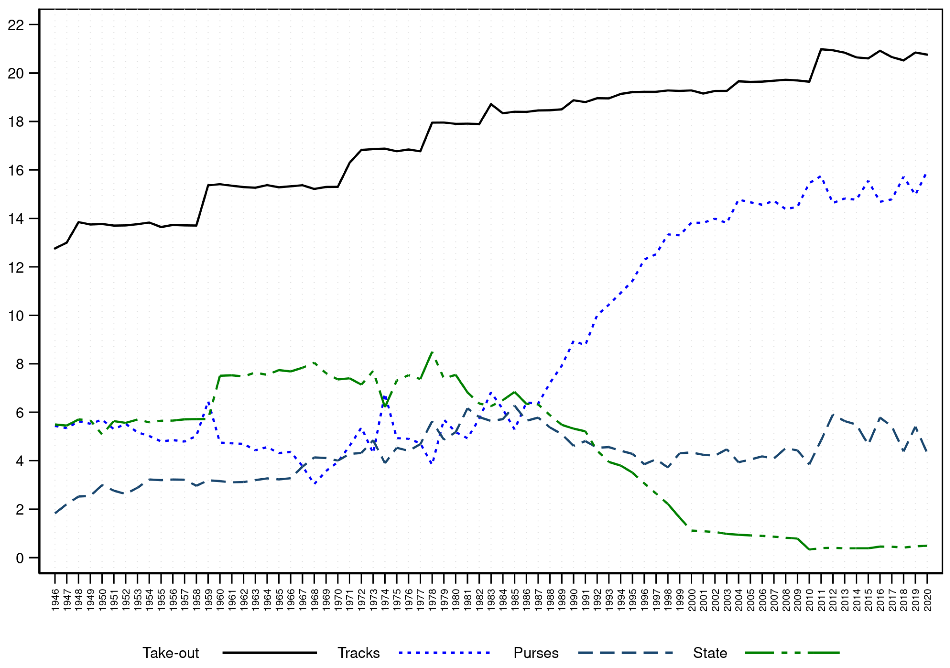
| 4 | By the late 1800s, there were over 300 racetracks in operations across the U.S. Bookmaking was replaced with the regulated pari-mutuel betting system starting in 1908. Under the pari-mutuel wagering system, players bet on random outcomes and winners share, in proportion to their wagers, the pool of all bets net of the racetrack’s commissions and state taxes—the “take-out rate”. |
| 5 | Starting in the early 1980s, racetracks began offering Advance Deposit Wagering (ADW) accounts, which are similar to electronic brokerage accounts at financial institutions. The horse racing industry infrastructure supports betting from multiple states and internationally. For a detailed historical background see Liebman (2017). |
| 6 | Pari-mutuel betting institutions function in a similar manner as the financial system, fulfilling important services, as outlined in Merton (1995). Merton’s functional perspective framework rests on the premise that financial functions, such as fulfilling demand for games of chance, are stable over time and market institutions, including the gambling industry, evolve to serve such functions. |
| 7 | Relying on more recent data, Maggio et al. (2020) empirically demonstrate that consumption responds to changes in stock market returns. These authors suggest that households treat capital gains and dividends as separate sources of income and show that consumption is highly responsive to both. Furthermore, Chodorow-Reich et al. (2021) demonstrate that, in addition to consumption, changes in stock market wealth also affect employment and the real economy. |
| 8 | Kaplan (2002) notes that since the 1980’s, the racing industry has witnessed significant proliferation of such intermediaries, generating a large flow of funds into horse wagering. Apparently, these hedge funds rely on exotic wagers with low probability but high payouts, for instance, superfecta, and picking winners in multiple races. Such bets are similar to the purchase of deep out-of-the-money options. A successful strategy generates small steady losses with infrequent but large gains. It is important to note, however, that the ability of horse betting markets to absorb a large flow of funds is limited by the number of tracks and available races. There is also a long tradition of racetrack gamblers and handicappers, becoming traders and stock pickers, and vice versa. Warren Buffet and Charlie Munger are two prime examples of horse race handicappers that became stock pickers. |
| 9 | This is not surprising, as rising VIX likely signals higher volatility of lottery-stocks and more skewed returns. Rising realized stock market volatility is unlikely to impact gambling payoffs at racetracks. |
| 10 | Under cumulative prospect theory, gamblers may act in a risk-loving manner as a consequence of over weighting small probability outcomes. On the application of prospect theory to gambling, see Barberis (2012) and Barberis (2013) and for a survey of economic models of risk aversion, see O’Donoghue and Somerville (2018) and their references. |
| 11 | As Conlisk (1993) has shown, this perspective is also consistent with the expected utility model. All that is needed to adequately explain the individual’s demand for gambles is a tiny felicity of gambling appended to any proposed utility function. For an interesting application of felicity of gambling in the horse wagering context see Green et al. (2020). |
| 12 | It is impossible to incorporate illegal wagering among individuals or through bookmakers in our analysis. In any case, the magnitude of illegal wagering likely dwindled as telephone and simulcast betting were introduced, starting in 1980’s. |
| 13 | Detailed historical information about these tracks and their Media Guides are available at https://www.dmtc.com/ and https://www.santaanita.com/, both accessed on 29 May 2023. After the Pearl Harbor attack (1941), both racetracks were closed (1942–1945) and were used as temporary internment camps for Japanese Americans. |
| 14 | The data for Del Mar Racetrack is available starting in 1938, its first operating year, resulting in 79 observations. |
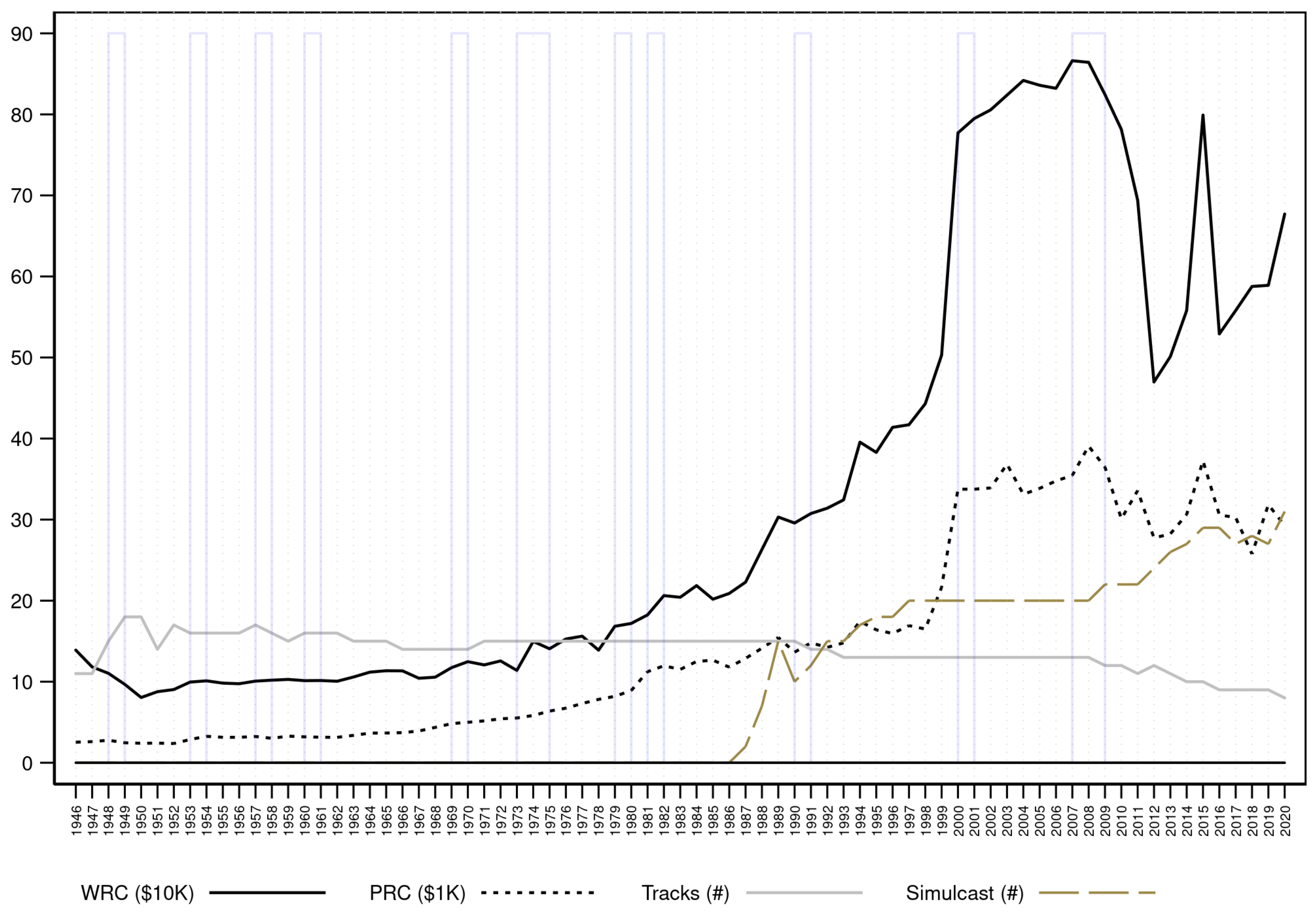
| 15 | Over the long span of time we study, the per capita wager in California has declined because the cumulative growth rate of the population, which is always positive with little variability, mostly exceeds the cumulative growth rate of aggregate wagers, which is subject to large positive and negative annual fluctuations. |
| 16 | History of gambling in California is detailed in Atkinson (1998) and California Legislative Analyst Office (2019). |
| 17 | Gramm et al. (2007) note similar trends across the United States: “From 1985 to 2002, the total wagered on Thoroughbred races in North America increased from $8.25 billion to $15.62 billion, despite the fact that the number of races dropped over 20 percent.” |
| 18 | In response to falling aggregate wagers, a host of new wagering products are introduced during this period. These include, exchange wagering (direct bettor to bettor wagers); futures wagering; track-subsidized and guaranteed wagering pools; wagering on the success rate of jockeys or trainers; take-out rebates to larger bettors; fantasy horse racing; wagering on previously-run races; and the ability to include fixed-odds wagering. |
| 19 | Surprisingly, during the COVID-19 pandemic, aggregate wagering on California races nearly matched its 2019 level, despite an 18% decline in the number of races. A similar phenomenon occurred for the U.S. as a whole. |
| 20 | Chiappori and Ekeland (2011) provide a detailed discussion of aggregate demand functions and the required assumptions for summing demand across individuals. |
| 21 | The specification in (1) and its logarithmic variants are popular in several areas of empirical economics; for example, estimation of CES-type production (utility, cost, other) functions. Following the introduction of the Box-Cox transformation, the search for “optimal variable transformation” has produced several useful methods to linearize Equation (1), as discussed in a recent survey by Atkinson et al. (2021). |
| 22 | See Grote and Matheson (2013) for a survey of the empirical literature and elasticity estimates for a variety of gambling activities, including horse wagering and lottery. |
| 23 | Modeling and interpreting linear and nonlinear interaction affects are discussed in Balli and Sørensen (2013) and Greene (2010). |
| 24 | While it is possible to model interaction effects by using the product of s and , our proposed specification provides better fits for the distribution of R. As Equation (3) shows, the term essentially acts as a weighting function that adjusts s over the range of . As seen below, this structure captures the dynamics of quite well. |
| 25 | We utilize the current realized excess returns, i.e., the current “premium” relative to the risk-free rate. In contrast, “equity risk premium” is typically estimated from long time series (Siegel 2017). We refrain from using the term “premium”, because it is often associated with expectations, rather than a single period of realized excess returns. |
| 26 | CRSP-VW and S&P-500 indexes are obtained from Wharton Research Data Services (https://wrds-www.wharton.upenn.edu/). Shiller’s total market returns are obtained from Yale University (http://www.econ.yale.edu/~shiller/data.htm). We also considered the Dow Industrial index. While we obtained similar results, we believe comparisons with the Dow is problematic because the Dow is a price-weighted index and has few constituents (30 stocks), and additions/deletions to this index are less reflective of the state of the economy. In any case, using the Dow will not change our results because it is highly correlated with the S&P 500 and CRSP indexes. The treasury bill data (https://fred.stlouisfed.org/series/TB3MS) and the monthly Aaa and Baa bond yields (https://fred.stlouisfed.org/series/AAA) are obtained from the Federal Reserve Bank of St. Louis. (These sources were last accessed on 29 May 2023). |
| 27 | Relative to a “recession dummy”, bond spread is more informative, as its magnitude captures the extent of recession or expansion. |
| 28 | Another measure of the credit market condition is the term spread, defined as the yield difference between corporate and treasury bonds with similar maturity. However, as Duca (1999) has shown, the term spread is a less informative measure due to the differences in the associated bonds’ covenants, for example callability provisions. The quality spread uses bonds with similar covenants and maturity, and is therefore subject to fewer complications arising from provisions that result in differential prepayment risk. Note that the quality spread is simply the difference between the term spreads of Baa and Aaa bonds relative to treasuries. |
| 29 | Under the current California law, at least 50% of the total sales revenues must be returned to the public in the form of prizes (take-out rate of 50%) and the remainder will be used to support public education (37%) and cover the lottery’s administrative costs (maximum of 13%). |
| 30 | We obtain the California annual per capita income from Federal Reserve Bank of St. Louis, https://fred.stlouisfed.org/series/CAPCPI, accessed on 29 May 2023. |
| 31 | We also considered the effect of the state unemployment rate. However, the coefficient is not significant and it is highly correlated with income. We therefore dropped unemployment rate from the estimation. |
| 32 | At off-track betting sites, races are simulcast from different tracks, allowing patrons to bet on a multitude of races. Nationwide, the ability to bet on horse races dramatically increased when off-track betting was legalized, first in New York (1970), and subsequently in other states. A second expansion of betting opportunities was brought about by inter-track wagering (simulcasts from one track to another). It is interesting to note that, Schwab implemented TeleBroker, the first trading application using the phone in 1989, nearly two decades after horse wagering by phone started in 1971. |
| 33 | Olmstead et al. (2007) estimate a water demand function in which price elasticity is conditional on the prevailing price structure, i.e., pricing is nonlinear such that higher marginal prices are charged for higher quantities consumed. Non-linearity arises from the fact the quantity consumed is conditional on individual’s “consumption block”, where different blocks have their own marginal pricing scheme. |
| 34 | Estimation results for the levels specification (Equation (1)) are consistent with the results for percent change specification (Equation (2)). However, the levels model suffers from major statistical shortcomings and biased coefficient estimates, as noted earlier. The results for levels specification are available upon request. |
| 35 | In the special case where errors in the nonlinear model are homoskedastic and orthogonal, NLS is efficient among estimators that only require the first two moments of residuals distribution (Cameron and Trivedi 2005). The percent change specification is more likely to be consistent with these requirements. |
| 36 | In the context of nonlinear models, the usefulness of adjusted has been a subject of debate. The row labeled “Fit” in the tables reports the squared correlation between the dependent variable and the model’s predicted values, and serves an alternative goodness-of-fit metric for nonlinear models. |
| 37 | For an interesting historical exposé regarding horse wagering during the Great Depression, see https://www.pbs.org/wgbh/americanexperience/features/seabiscuit-racing-depression/, accessed on 29 May 2023. |
| 38 | We included a dummy variable for each tail separately, but the estimated coefficients remained unchanged. We opted for a symmetrical “Tail Impact” to keep the models parsimonious and save degrees of freedom. |
References
- Arthur, Jennifer N., Robert J. Williams, and Paul H. Delfabbro. 2016. The conceptual and empirical relationship between gambling, investing, and speculation. Journal of Behavioral Addictions 5: 580–91. [Google Scholar] [CrossRef] [Green Version]
- Atkinson, Anthony C., Marco Riani, and Aldo Corbellini. 2021. The Box–Cox Transformation: Review and Extensions. Statistical Science 36: 239–55. [Google Scholar] [CrossRef]
- Atkinson, Megan M. 1998. Gambling in California: An Overview. Legislative Analyst’s Office-An LAO Report. Sacramento: State of California. [Google Scholar]
- Baker, Malcolm, and Jeffrey Wurgler. 2007. Investor sentiment in the stock market. Journal of Economic Perspectives 21: 129–51. [Google Scholar] [CrossRef] [Green Version]
- Balli, Hatice Ozer, and Bent E. Sørensen. 2013. Interaction effects in econometrics. Empirical Economics 45: 583–603. [Google Scholar] [CrossRef] [Green Version]
- Barber, Brad M., Yi-Tsung Lee, Yu-Jane Liu, and Terrance Odean. 2009. Just how much do individual investors lose by trading? Review of Financial Studies 22: 609–32. [Google Scholar] [CrossRef]
- Barberis, Nicholas. 2012. A model of casino gambling. Management Science 58: 35–51. [Google Scholar] [CrossRef] [Green Version]
- Barberis, Nicholas. 2013. Thirty years of prospect theory in economics: A review and assessment. Journal of Economic Perspectives 27: 173–96. [Google Scholar] [CrossRef] [Green Version]
- California Horse Racing Board. 1934–2021. Annual Reports (Various Annual and Biannual Issues); Sacramento: California Horse Racing Board. Available online: http://www.chrb.ca.gov/annual_reports.asp (accessed on 29 May 2023).
- California Legislative Analyst Office. 2019. Overview of Gambling in California; Sacramento: California Legislative Analyst Office. Available online: https://lao.ca.gov/handouts/crimjust/2019/Gambling-Overview-022619.pdf (accessed on 29 May 2023).
- Cameron, Colin, and Pravin Trivedi. 2005. Microeconometrics: Methods and Applications. New York: Cambridge University Press. [Google Scholar]
- Chen, Yao, Alok Kumar, and Chendi Zhang. 2021. Searching for gambles: Gambling sentiment and stock market outcomes. Journal of Financial and Quantitative Analysis 56: 2010–38. [Google Scholar] [CrossRef]
- Chiappori, Pierre-André, and Ivar Ekeland. 2011. New developments in aggregation economics. Annual Review of Economics 3: 631–68. [Google Scholar] [CrossRef] [Green Version]
- Chiappori, Pierre-André, Bernard Salanié, François Salanié, and Amit Gandhi. 2019. From aggregate betting data to individual risk preferences. Econometrica 87: 1–36. [Google Scholar] [CrossRef]
- Chodorow-Reich, Gabriel, Plamen T. Nenov, and Alp Simsek. 2021. Stock market wealth and the real economy: A local labor market approach. American Economic Review 111: 1613–57. [Google Scholar] [CrossRef]
- Conlisk, John. 1993. The utility of gambling. Journal of Risk and Uncertainty 6: 255–75. [Google Scholar] [CrossRef]
- DeGennaro, Ramon P., and Ann B. Gillette. 2013. The modern racing landscape and the racetrack wagering market: Components of demand, subsidies and efficiency. In Oxford Handbook of the Economics of Gambling. Edited by Leighton Vaughan Williams and Donald S. Siegel. Oxford: Oxford University Press. [Google Scholar]
- Dorn, Daniel, Anne Jones Dorn, and Paul Sengmueller. 2014. Trading as gambling. Management Science 61: 2376–93. [Google Scholar] [CrossRef]
- Dorn, Daniel, and Paul Sengmueller. 2009. Trading as entertainment? Management Science 55: 591–603. [Google Scholar] [CrossRef]
- Duca, John V. 1999. What credit market indicators tell us. Economic and Financial Review, Federal Reserve Bank of Dallas. Available online: https://www.dallasfed.org/~/media/documents/research/efr/1999/efr9903a.pdf (accessed on 29 May 2023).
- Fama, Eugene F., and Kenneth R. French. 1989. Business conditions and expected returns on stocks and bonds. Journal of Financial Economics 25: 23–49. [Google Scholar] [CrossRef]
- Faust, Jon, Simon Gilchrist, Jonathan H. Wright, and Egon Zakrajsek. 2013. Credit spreads as predictors of real-time economic activity: A bayesian model-averaging approach. The Review of Economics and Statistics 95: 1501–19. [Google Scholar] [CrossRef] [Green Version]
- Gao, Xiaohui, and Tse-Chun Lin. 2015. Do individual investors treat trading as a fun and exciting gambling activity? Evidence from repeated natural experiments. Review of Financial Studies 28: 2128–66. [Google Scholar] [CrossRef] [Green Version]
- Gomber, Peter, Peter Rohr, and Uwe Schweickert. 2008. Sports betting as a new asset class—Current market organization and options for development. Financial Markets and Portfolio Management 22: 169–92. [Google Scholar] [CrossRef]
- Gramm, Marshall, Nicholas Mckinney, Douglas H. Owens, and Matt E. Ryan. 2007. What do bettors want? determinants of pari-mutuel betting preference. American Journal of Economics and Sociology 66: 465–91. [Google Scholar] [CrossRef]
- Green, Etan, Haksoo Lee, and David M. Rothschild. 2020. The favorite-longshot midas. Social Science Research Network. Available online: https://papers.ssrn.com/sol3/papers.cfm?abstract_id=3271248 (accessed on 29 May 2023).
- Greene, William. 2010. Testing hypotheses about interaction terms in nonlinear models. Economics Letters 107: 291–96. [Google Scholar] [CrossRef] [Green Version]
- Grinblatt, Mark, and Matti Keloharju. 2009. Sensation seeking, overconfidence, and trading activity. Journal of Finance 64: 549–78. [Google Scholar] [CrossRef] [Green Version]
- Grote, Kent, and Victor A. Matheson. 2013. The economics of lotteries: A survey of the literature. In Oxford Handbook of the Economics of Gambling. Oxford: Oxford University Press. [Google Scholar]
- Gruen, Arthur. 1976. An inquiry into the economics of race-track gambling. Journal of Political Economy 84: 169–78. [Google Scholar] [CrossRef]
- Guzman, Martin, and Joseph E. Stiglitz. 2021. Pseudo-wealth and consumption fluctuations. The Economic Journal 131: 372–91. [Google Scholar] [CrossRef]
- Harville, David A. 1973. Assigning probabilities to the outcomes of multi-entry competitions. Journal of the American Statistical Association 68: 312–16. [Google Scholar] [CrossRef]
- Herskowitz, Sylvan. 2021. Gambling, saving, and lumpy liquidity needs. American Economic Journal: Applied Economics 13: 72–104. [Google Scholar] [CrossRef]
- Jaffee, Dwight M. 1975. Cyclical variations in the risk structure of interest rates. Journal of Monetary Economics 1: 309–25. [Google Scholar] [CrossRef]
- Kang, Johnny, and Carolin E. Pflueger. 2015. Inflation risk in corporate bonds. Journal of Finance 70: 115–62. [Google Scholar] [CrossRef] [Green Version]
- Kaplan, Michael. 2002. The high tech trifecta. Wired Magazine 10: 10–13. [Google Scholar]
- Kumar, Alok. 2009. Who gambles in the stock market? Journal of Finance 64: 1889–933. [Google Scholar] [CrossRef]
- Kumar, Alok, Thanh H. Nguyen, and Talis J. Putnins. 2021. Stock Market Gambling around the World and Market Efficiency. Available online: https://ssrn.com/abstract=3686393 (accessed on 29 May 2023).
- Leuz, Christian, Steffen Meyer, Maximilian Muhn, Eugene F. Soltes, and Andreas Hackethal. 2021. Who Falls Prey to the Wolf of Wall Street? Investor Participation in Market Manipulation. Center for Financial Studies Working Paper No. 609. Available online: https://ssrn.com/abstract=3289931 (accessed on 29 May 2023).
- Liebman, Bennett. 2017. Pari-mutuels: What do they mean and what is at stake in the 21st century. Marquette Sports Law Review 27: 45–111. [Google Scholar]
- Maggio, Marco Di, Amir Kermani, and Kaveh Majlesi. 2020. Stock market returns and consumption. Journal of Finance 75: 3175–219. [Google Scholar] [CrossRef]
- Manning, Willard G., and John Mullahy. 2001. Estimating log models: To transform or not to transform? Journal of Health Economics 20: 461–94. [Google Scholar] [CrossRef] [PubMed] [Green Version]
- Merton, Robert C. 1995. A functional perspective of financial intermediation. Financial Management 24: 23–41. [Google Scholar] [CrossRef]
- Mosenhauer, Moritz, Philip W. S. Newall, and Lukasz Walasek. 2021. The stock market as a casino: Associations between stock market trading frequency and problem gambling. Journal of Behavioral Addictions 10: 683–689. [Google Scholar] [CrossRef]
- O’Donoghue, Ted, and Jason Somerville. 2018. Modeling risk aversion in economics. Journal of Economic Perspectives 32: 91–114. [Google Scholar] [CrossRef] [Green Version]
- Olmstead, Sheila M., Michael Hanemann, and Robert N. Stavins. 2007. Water demand under alternative price structures. Journal of Environmental Economics and Management 54: 181–98. [Google Scholar] [CrossRef] [Green Version]
- Poterba, James M. 2000. Stock market wealth and consumption. Journal of Economic Perspectives 14: 99–118. [Google Scholar] [CrossRef]
- Ramezani, Cyrus, and James Ahern. 2022. Business Cycles, Stock Market Wealth and Gambling at the Racetracks. Social Science Research Network. Available online: https://papers.ssrn.com/sol3/papers.cfm?abstract_id=4386429 (accessed on 29 May 2023).
- Riess, Steven. 2014. The cyclical history of horse racing: The USA’s oldest and (sometimes) most popular spectator sport. Journal of the History of Sport 31: 29–54. [Google Scholar] [CrossRef]
- Santos-Silva, J. M. C., and Silvana Tenreyro. 2006. The log of gravity. Review of Economics and Statistics 88: 641–658. [Google Scholar] [CrossRef] [Green Version]
- Sauer, Raymond D. 1998. The economics of wagering markets. Journal of Economic Literature 36: 2021–64. [Google Scholar]
- Schwartz, David G. 2013. Roll the Bones: The History of Gambling. New York: Winchester Books. [Google Scholar]
- Schwert, G. William. 1989. Why does stock market volatility change over time? Journal of Finance 44: 1115–53. [Google Scholar] [CrossRef]
- Siegel, Laurence B. 2017. The equity risk premium: A contextual literature review. CFA Institute Research Foundation 12: 1–30. Available online: https://ssrn.com/abstract=3088820 (accessed on 29 May 2023). [CrossRef] [Green Version]
- Simmons, Susan A., and Robert Sharp. 1987. State lotteries’ effects on thoroughbred horse racing. Journal of Policy Analysis and Management 6: 446–48. [Google Scholar] [CrossRef]
- Snowberg, Erik, and Justin Wolfers. 2010. Explaining the favorite–long shot bias: Is it risk-love or misperceptions? Journal of Political Economy 118: 723–46. [Google Scholar] [CrossRef] [Green Version]
- Suits, Daniel B. 1979. The elasticity of demand for gambling. Quarterly Journal of Economics 93: 155–62. [Google Scholar] [CrossRef]
- Thalheimer, Richard, and Mukhtar M. Ali. 1995. The demand for parimutuel horse race wagering and attendance. Management Science 41: 129–43. [Google Scholar] [CrossRef]
- Weidner, Linus. 2022. Gambling and financial markets a comparison from a regulatory perspective. Frontiers in Sociology 7: 1–5. [Google Scholar] [CrossRef]
- Zhang, Zhiwei. 2002. Corporate Bond Spreads and the Business Cycle. Bank of Canada Working Paper, 2002–2015. Ottawa: Bank of Canada. [Google Scholar]
- Ziemba, William T. 2021. Parimutuel Betting Markets: Racetracks and Lotteries Revisited. Discussion Paper No 103. London: Systemic Risk Centre, The London School of Economics and Political Science. Available online: https://papers.ssrn.com/sol3/papers.cfm?abstract_id=3865785 (accessed on 29 May 2023).


| Dependent Variables | |
|---|---|
| (% Change in WRC) | Wager Per Race, (WRC, $) |
| WRC = Aggregate Wagers/number of races, by year | |
| Similarly defined for Del Mar and Santa Anita Tracks | |
| Explanatory Variables | |
| Financial Market Outcomes and Lottery | |
| Bond Spread | Average of Moody’s Monthly Yield Spread (Baa-AAA) |
| CRSP-VW Premium | Average of Monthly CRSP-VW Excess Returns |
| CRSP-VW Volatility | Standard Deviation of Monthly CRSP-VW Returns |
| S&P Premium | Average of Monthly S&P-500 Excess Returns |
| S&P Volatility | Standard Deviation of Monthly S&P-500 Returns |
| Shiller Premium | Average of Monthly Shiller’s Excess Returns |
| Shiller Volatility | Standard Deviation of Shiller’s Monthly Returns |
| Lottery | California Lottery Dummy Variable |
| Economic and Racing Industry Variables | |
| Price (Take-out Rate) | Fraction of Aggregate Wagers distributed to racetracks, |
| horse owners and taxes. | |
| Income, $ | California Income deflated by Population |
| Purse per Race, $ | Purse Proceeds / number of races |
| Off-Track Wager | Fraction of Aggregate Wagers originating from off-track facilities |
| Purse Proceeds, $ | Aggregate Dollars distributed to horse owners, $ |
| Track Proceeds, $ | Aggregate Dollars distributed to racetracks & affiliated businesses |
| Relative Incentive | Purse Proceeds / Track Proceeds |
| Relative Compensation Index | RCI = (Relative Incentive) × (number of operating racetracks) |
| Mean | St. Dev. | Skewness | Kurtosis | Min | Max | |
|---|---|---|---|---|---|---|
| Dependent Variables | ||||||
| Wager Per Race-California ($) | 309,383 | 268,865 | 0.93 | 2.40 | 18,627 | 866,227 |
| (% Change in WRC) | 0.05 | 0.15 | 1.01 | 6.30 | −0.34 | 0.57 |
| -Del Mar (N = 79) | 0.05 | 0.13 | 1.90 | 12.93 | −0.30 | 0.74 |
| -Santa Anita | 0.04 | 0.13 | 0.84 | 8.30 | −0.42 | 0.61 |
| Explanatory Variables | ||||||
| Financial Market Outcomes and Lottery | ||||||
| Bond Spreads—(Baa-AAA) | 0.01 | 0.00 | 1.35 | 4.46 | 0.00 | 0.03 |
| CRSP-VW Excess Returns | 0.08 | 0.16 | −0.38 | 3.12 | −0.35 | 0.45 |
| CRSP-VW Market Volatility | 0.04 | 0.02 | 1.84 | 8.16 | 0.02 | 0.13 |
| S&P Excess Returns | 0.05 | 0.15 | −0.37 | 3.21 | −0.38 | 0.45 |
| S&P Market Volatility | 0.04 | 0.02 | 2.17 | 9.96 | 0.02 | 0.14 |
| Shiller Excess Returns | 0.03 | 0.17 | −0.37 | 2.94 | −0.36 | 0.40 |
| Shiller Market Volatility | 0.03 | 0.02 | 1.36 | 4.61 | 0.01 | 0.08 |
| Lottery Dummy | 0.44 | 0.50 | 0.22 | 1.05 | 0.00 | 1.00 |
| Economic and Racing Industry Variables | ||||||
| Price (Per $ of Wager) | 0.17 | 0.03 | −0.22 | 1.65 | 0.12 | 0.21 |
| % Change in Price | 0.01 | 0.03 | 0.93 | 9.44 | −0.09 | 0.12 |
| Income($) | 19,248 | 19,391 | 0.96 | 2.80 | 776 | 71,261 |
| % Change in Income | 0.05 | 0.04 | 0.82 | 6.04 | −0.04 | 0.21 |
| Purse (Per $ of Wager) | 0.04 | 0.01 | 0.08 | 2.26 | 0.02 | 0.06 |
| Track (Per $ of Wager) | 0.08 | 0.04 | 0.58 | 1.62 | 0.03 | 0.16 |
| Purse Proceeds/Track Proceeds | 0.60 | 0.29 | 0.89 | 3.06 | 0.25 | 1.47 |
| Number of Tracks—California | 14 | 2.22 | −0.55 | 3.35 | 8 | 19 |
| Relative Compensation Index (RCI) | 8.63 | 4.73 | 0.59 | 2.51 | 2.17 | 22.03 |
| Purse Per Race (PRC) ($) | 13,790 | 12,327 | 0.73 | 2.02 | 585 | 39,068 |
| % Change in PRC | 0.05 | 0.13 | 1.52 | 7.24 | −0.18 | 0.56 |
| % Change in PRC—Del Mar (N = 79) | 0.05 | 0.11 | 1.00 | 9.47 | −0.37 | 0.56 |
| % Change in PRC—Santa Anita | 0.05 | 0.17 | 0.78 | 5.89 | −0.46 | 0.62 |
| Number of Races | 6107 | 2430 | 0.24 | 1.89 | 2113 | 10,590 |
| % Change in Number of Races (NRC) | 0.01 | 0.11 | 0.92 | 9.91 | −0.33 | 0.47 |
| % Change in NRC—Del Mar (N = 79) | 0.01 | 0.10 | 2.37 | 14.39 | −0.32 | 0.48 |
| % Change in NRC—Santa Anita | 0.01 | 0.11 | 1.94 | 12.81 | −0.36 | 0.56 |
| Off-Track Wager (Fraction of Wagers) | 0.31 | 0.39 | 0.55 | 1.41 | 0.00 | 0.93 |
| % Change in Off-Track Wager | 0.01 | 0.03 | 5.35 | 35.48 | −0.00 | 0.25 |
| Explanatory Variables | s (S&P) | and | s | Static | S&P | CRSP | Schiller |
|---|---|---|---|---|---|---|---|
| Financial Market Outcomes and Lottery | |||||||
| Bond-Spread | 4.130 | 3.917 | 7.190 *** | 7.215 *** | 6.308 ** | ||
| 0.98 | 1.66 | 3.96 | 3.56 | 2.30 | |||
| Excess Returns | 0.015 | −0.082 | −0.154 ** | −0.123 * | −0.092 | ||
| 0.13 | −0.93 | −2.23 | −1.87 | −1.22 | |||
| Market Volatility | 0.128 | −1.231 | −1.793 *** | −1.679 ** | −1.814 *** | ||
| 0.13 | −1.52 | −2.80 | −2.50 | −2.81 | |||
| California Lottery | −0.004 | −0.014 | −0.059 ** | −0.064 ** | −0.069 *** | ||
| Dummy Var. | −0.12 | −0.79 | −2.55 | −2.59 | −2.73 | ||
| Economic and Racing Industry Variables | |||||||
| Price | −0.77 | −0.678 | −2.402 ** | −2.449 ** | −2.330 ** | ||
| −1.28 | −1.17 | −2.34 | −2.38 | −2.01 | |||
| Income | 1.00 *** | 0.877 ** | 2.593 *** | 2.646 *** | 2.689 *** | ||
| 3.07 | 2.18 | 4.52 | 4.40 | 3.99 | |||
| Purse per Race | 0.653 *** | 0.543 *** | 0.921 *** | 0.927 *** | 0.880 *** | ||
| 5.83 | 4.87 | 3.68 | 3.42 | 3.32 | |||
| Number of Races | −0.452 *** | −0.549 *** | −0.741 *** | −0.757 *** | −0.836 *** | ||
| −4.57 | −6.16 | −7.86 | −7.78 | −7.04 | |||
| Off Track Wager | 0.438 *** | 0.488 *** | 2.168 * | 2.223 * | 2.276 * | ||
| 4.38 | 2.83 | 1.96 | 1.91 | 1.69 | |||
| Relative Comp. Index | −0.103 *** | −0.107 *** | −0.114 *** | ||||
| RCI | −2.99 | −2.91 | −3.06 | ||||
| Model Diagnostics | |||||||
| Adj. R | 0.06 | 0.16 | 0.61 | 0.67 | 0.73 | 0.72 | 0.71 |
| Fit | 0.02 | 0.09 | 0.59 | 0.67 | 0.74 | 0.73 | 0.72 |
| Serial Correlation (p-value) | 0.89 | 0.58 | 0.17 | 0.34 | 0.63 | 0.57 | 0.46 |
| Normality (p-value) | 0.00 | 0.00 | 0.00 | 0.04 | 0.32 | 0.16 | 0.25 |
| Log-Likelihood | 42 | 45 | 77 | 87 | 96 | 95 | 93 |
| AIC | −76 | −87 | −147 | −155 | −172 | −170 | −166 |
| BIC | −67 | −82 | −140 | −134 | −148 | −146 | −142 |
| Num. of Iterations | - | - | - | - | 19 | 22 | 30 |
| Explanatory Variables | Del Mar | Santa Anita | ||||
|---|---|---|---|---|---|---|
| S&P | CRSP | Schiller | S&P | CRSP | Schiller | |
| Financial Market Outcomes and Lottery | ||||||
| Bond-Spread | 0.494 | 1.199 | 0.251 | 7.200 ** | 7.073 ** | 6.104 ** |
| 0.20 | 0.47 | 0.08 | 2.42 | 2.35 | 2.25 | |
| Excess Returns | −0.103 | −0.062 | −0.052 | −0.06 | −0.067 | −0.042 |
| −1.51 | −1.04 | −0.84 | −0.93 | −1.03 | −0.60 | |
| Market Volatility | −0.538 | −0.688 | −0.438 | −1.089 | −1.01 | −0.937 |
| −0.71 | −0.91 | −0.47 | −1.40 | −1.32 | −1.25 | |
| California Lottery | −0.034 | −0.037 | −0.039 | −0.057 ** | −0.059 ** | −0.062 ** |
| Dummy Var. | −1.52 | −1.59 | −1.64 | −2.06 | −2.15 | −2.24 |
| Economic and Racing Industry Variables | ||||||
| Price | −0.622 | −0.672 | −0.590 | −2.111 | −2.139 | −2.170 |
| −1.22 | −1.21 | −1.03 | −1.14 | −1.15 | −1.01 | |
| Income | 1.116 ** | 1.104 ** | 1.007 ** | 1.632 | 1.742 | 1.779 |
| 2.29 | 2.22 | 2.03 | 1.59 | 1.63 | 1.48 | |
| Purse per Race | 0.535 *** | 0.535 *** | 0.520 *** | 1.092 ** | 1.112 ** | 1.169 ** |
| 8.25 | 7.84 | 7.37 | 2.49 | 2.51 | 2.27 | |
| Number of Races | −0.359 ** | −0.358 ** | −0.349 * | 0.143 | 0.132 | 0.152 |
| −2.07 | −2.05 | −1.90 | 0.29 | 0.26 | 0.27 | |
| Off Track Wager | 1.859 *** | 1.905 *** | 1.873 ** | 2.264 | 2.322 | 2.639 |
| 2.77 | 2.74 | 2.50 | 1.42 | 1.43 | 1.36 | |
| Relative Comp. Index | −0.008 | −0.008 | −0.008 | −0.185 ** | −0.188 ** | −0.207 ** |
| RCI | −0.42 | −0.41 | −0.37 | −2.44 | −2.46 | −2.27 |
| Model Diagnostics | ||||||
| Adj. R | 0.69 | 0.69 | 0.68 | 0.47 | 0.47 | 0.46 |
| Fit | 0.68 | 0.68 | 0.68 | 0.50 | 0.50 | 0.49 |
| Serial Correlation (p-value) | 0.50 | 0.43 | 0.32 | 0.21 | 0.22 | 0.26 |
| Normality (p-value) | 0.17 | 0.05 | 0.05 | 0.49 | 0.57 | 0.46 |
| Log-Likelihood | 95 | 95 | 94 | 79 | 79 | 79 |
| AIC | −170 | −169 | −168 | −139 | −139 | −137 |
| BIC | −146 | −146 | −144 | −115 | −115 | −113 |
| Num. of Iterations | 16 | 16 | 19 | 21 | 21 | 23 |
| Explanatory Variables | California | Del Mar | Santa Anita | ||
|---|---|---|---|---|---|
| S&P | CRSP | Schiller | S&P | S&P | |
| Financial Market Outcomes and Lottery | |||||
| Tail Impact | 0.477 *** | 0.509 *** | 0.497 *** | 0.155 *** | 0.177 *** |
| 3.19 | 3.41 | 3.31 | 7.98 | 14.71 | |
| Bond-Spread | 6.015 *** | 6.130 *** | 4.861 * | 1.470 | 4.634 * |
| 3.19 | 3.03 | 1.97 | 0.83 | 1.89 | |
| Excess Returns | −0.129 * | −0.122 * | −0.081 | −0.058 | −0.014 |
| −1.92 | −1.84 | −1.10 | −1.36 | −0.29 | |
| Market Volatility | −1.490 ** | −1.414 ** | −1.351 * | 0.316 | −0.734 |
| −2.58 | −2.38 | −1.93 | 0.70 | −1.35 | |
| California Lottery | −0.052 ** | −0.055 ** | −0.060 ** | −0.019 | −0.020 |
| Dummy Var. | −2.22 | −2.33 | −2.28 | −1.34 | −0.89 |
| Economic and Racing Industry Variables | |||||
| Price | −2.072 * | −2.150 * | −2.045 * | −0.217 | −0.410 |
| −1.85 | −1.90 | −1.67 | −1.12 | −0.60 | |
| Income | 2.280 *** | 2.404 *** | 2.398 *** | 0.210 | 0.750 |
| 3.13 | 3.16 | 2.77 | 1.09 | 1.52 | |
| Purse per Race | 0.423 ** | 0.398 ** | 0.360 * | 0.154 ** | 0.363 ** |
| 2.25 | 2.12 | 1.70 | 2.34 | 2.22 | |
| Number of Races | −0.556 *** | −0.551 *** | −0.612 *** | −0.114 | 0.340 ** |
| −5.28 | −5.16 | −4.98 | −1.21 | 2.16 | |
| Off Track Wager | 1.985 * | 2.072 | 2.106 | 0.854 * | 0.084 |
| 1.67 | 1.66 | 1.46 | 1.96 | 0.35 | |
| Relative Comp. Index | −0.101 ** | −0.108 ** | −0.115 ** | 0.042 | −0.081 |
| RCI | −2.55 | −2.59 | −2.58 | 1.13 | −1.40 |
| Model Diagnostics | |||||
| Adj. R | 0.77 | 0.77 | 0.75 | 0.84 | 0.80 |
| Fit | 0.78 | 0.78 | 0.76 | 0.84 | 0.81 |
| Serial Correlation (p-value) | 0.44 | 0.35 | 0.21 | 0.80 | 0.37 |
| Normality (p-value) | 0.10 | 0.11 | 0.06 | 0.73 | 0.24 |
| Log-Likelihood | 102 | 102 | 100 | 123 | 119 |
| AIC | −183 | −183 | −178 | −223 | −215 |
| BIC | −157 | −157 | −151 | −197 | −189 |
| Num. of Iterations | 21 | 24 | 33 | 23 | 16 |
| Explanatory Variables | Simple | Improved | ||||
|---|---|---|---|---|---|---|
| S&P | CRSP | Schiller | S&P | CRSP | Schiller | |
| Financial Market Outcomes and Lottery | ||||||
| Tail Impact | 0.444 *** | 0.470 *** | 0.443 *** | |||
| 2.95 | 3.20 | 3.10 | ||||
| Bond-Spread | 22.748 *** | 25.492 *** | 30.416 *** | 17.438 ** | 19.775 ** | 23.819 ** |
| 3.02 | 3.40 | 3.10 | 2.06 | 2.36 | 2.10 | |
| Excess Returns | −0.323 | −0.286 | −0.236 | −0.282 | −0.310 | −0.223 |
| −1.65 | −1.50 | −1.09 | −1.30 | −1.46 | −0.90 | |
| Market Volatility | −4.334 ** | −4.451 *** | −5.669 *** | −3.412 * | −3.636 ** | −4.482 * |
| −2.51 | −2.65 | −2.83 | −1.84 | −2.02 | −1.89 | |
| California Lottery | −0.174 *** | −0.193 *** | −0.258 *** | −0.147 ** | −0.159 ** | −0.223 ** |
| Dummy Var. | −2.65 | −2.81 | −3.23 | −2.15 | −2.30 | −2.30 |
| Economic and Racing Industry Variables | ||||||
| Price | −3.405 *** | −3.556 *** | −3.892 *** | −2.952 ** | −3.122 ** | −3.478 ** |
| −3.39 | −3.69 | −3.46 | −2.40 | −2.60 | −2.48 | |
| Income | 3.284 *** | 3.381 *** | 3.662 *** | 3.000 *** | 3.217 *** | 3.444 *** |
| 4.58 | 4.33 | 4.33 | 2.94 | 3.11 | 2.81 | |
| Purse per Race | 0.996 *** | 0.991 *** | 0.874 *** | 0.478 ** | 0.443 ** | 0.356 |
| 4.50 | 4.51 | 3.59 | 2.17 | 2.18 | 1.59 | |
| Number of Races | −0.970 *** | −1.016 *** | −1.241 *** | −0.821 *** | −0.846 *** | −1.056 *** |
| −7.28 | −7.68 | −6.13 | −4.93 | −5.10 | −4.33 | |
| Off Track Wager | 2.607 ** | 2.651 ** | 3.072 * | 2.396 * | 2.446 * | 2.888 |
| 2.19 | 2.20 | 1.74 | 1.81 | 1.87 | 1.51 | |
| Relative Comp. Index | −0.138 *** | −0.144 *** | −0.161 *** | −0.137 *** | −0.144 *** | −0.165 *** |
| RCI | −4.48 | −4.69 | −4.14 | −3.30 | −3.57 | −3.29 |
| Model Diagnostics | ||||||
| Adj. R | 0.74 | 0.74 | 0.74 | 0.77 | 0.78 | 0.77 |
| Fit | 0.75 | 0.75 | 0.75 | 0.79 | 0.79 | 0.78 |
| Serial Correlation (p-value) | 0.59 | 0.53 | 0.52 | 0.33 | 0.24 | 0.25 |
| Normality (p-value) | 0.16 | 0.10 | 0.04 | 0.18 | 0.15 | 0.07 |
| Log-Likelihood | 98 | 98 | 97 | 104 | 104 | 103 |
| AIC | −176 | −175 | −174 | −185 | −187 | −184 |
| BIC | −152 | −151 | −150 | −159 | −160 | −158 |
| Num. of Iterations | 14 | 14 | 14 | 15 | 14 | 16 |
| Static | Simple | Improved | |||||||
|---|---|---|---|---|---|---|---|---|---|
| % Change | Mean | St. Dev. | Min | Max | Mean | St. Dev. | Min | Max | |
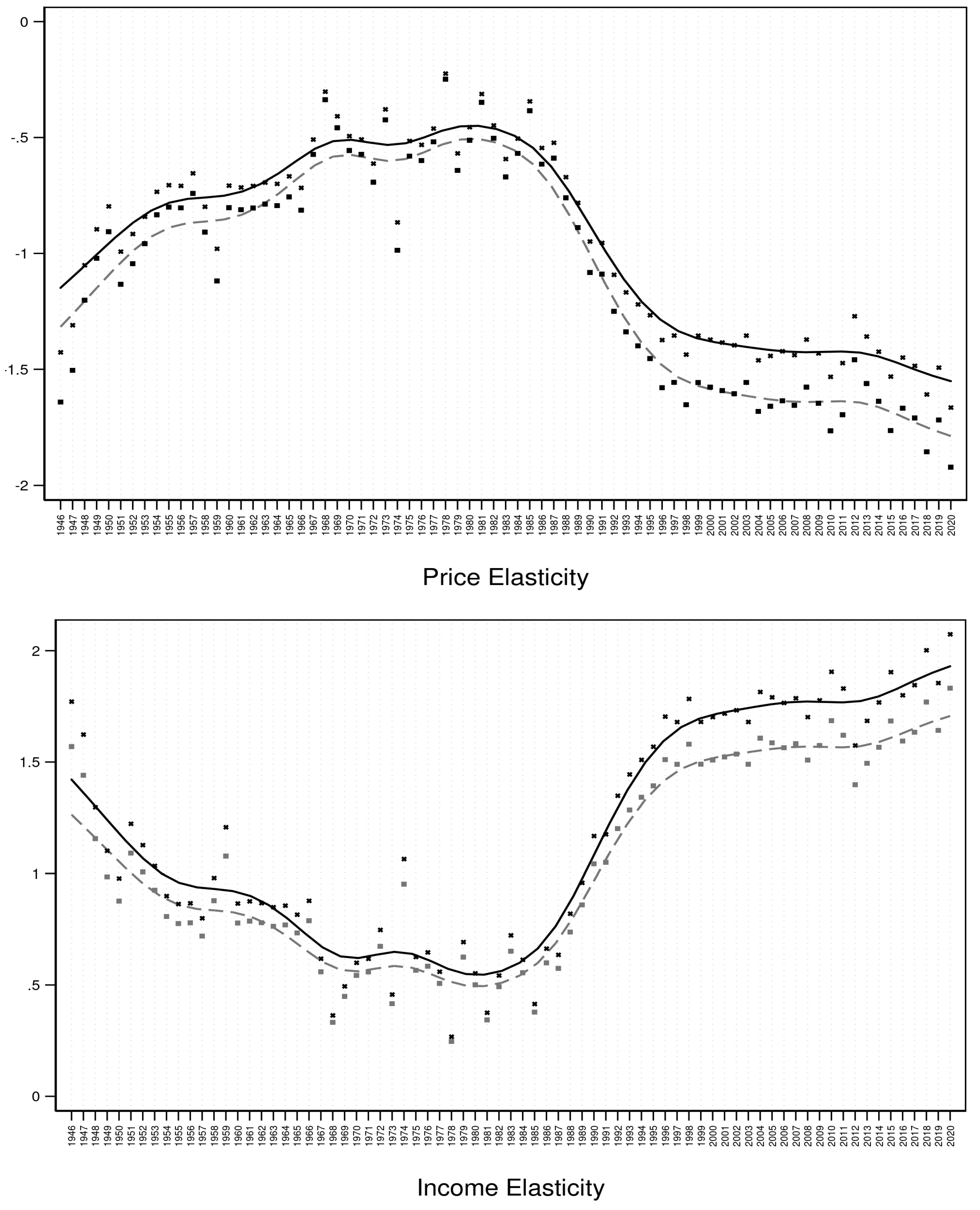
| Price | −0.68 | −1.10 *** | 0.46 | −1.92 | −0.25 | −0.96 ** | 0.40 | −1.66 | −0.22 |
| Income | 0.88 ** | 1.18 *** | 0.50 | 0.27 | 2.07 | 1.06 *** | 0.44 | 0.25 | 1.83 |
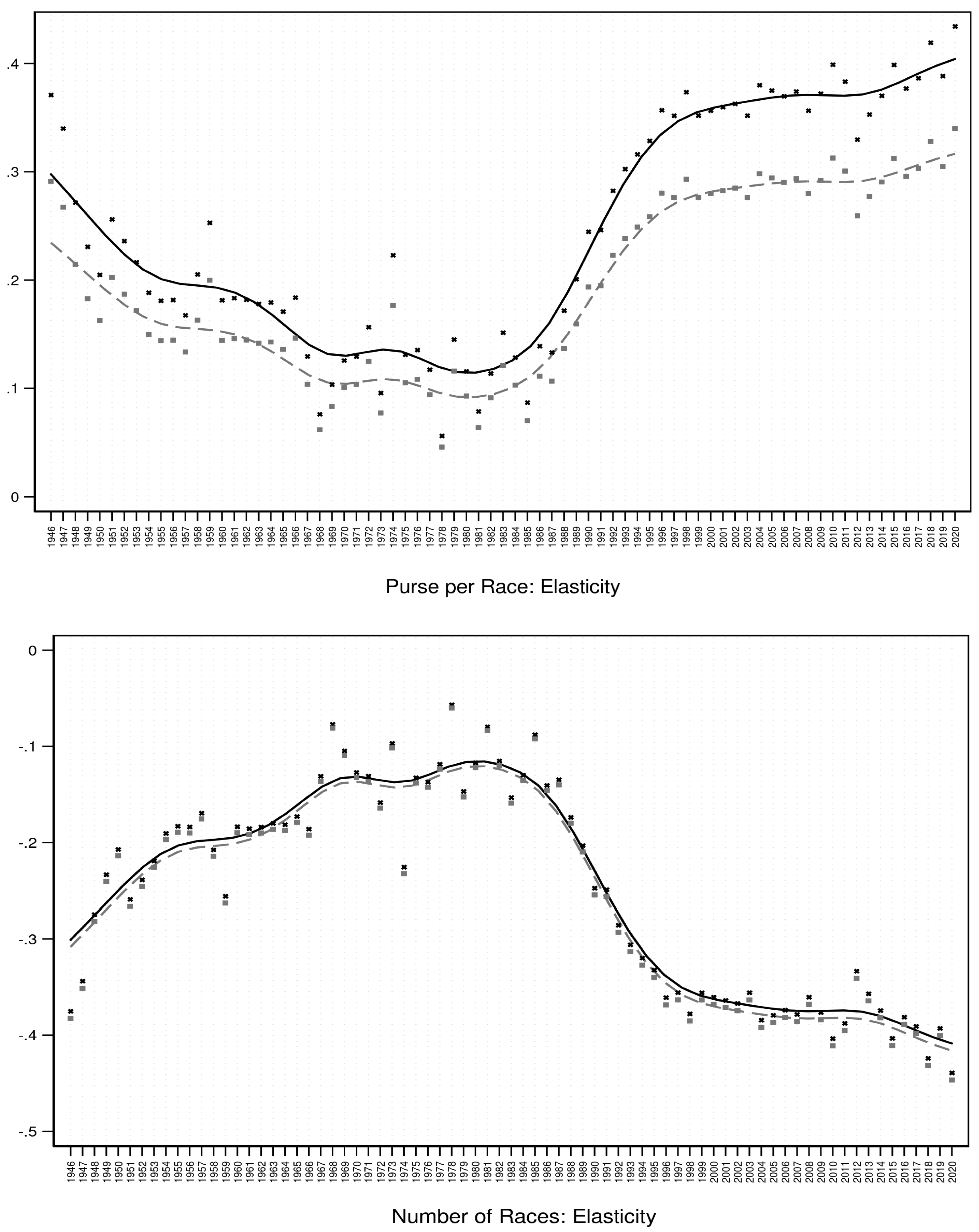
| PRC | 0.54 *** | 0.25 *** | 0.11 | 0.06 | 0.43 | 0.20 ** | 0.08 | 0.05 | 0.34 |
| No. of Races | −0.55 *** | −0.25 *** | 0.11 | −0.44 | −0.06 | −0.26 *** | 0.11 | −0.45 | −0.06 |
| Off-Track | 0.49 *** | 1.35 ** | 0.30 | 0.53 | 1.77 | 1.16 ** | 0.26 | 0.47 | 1.52 |
Disclaimer/Publisher’s Note: The statements, opinions and data contained in all publications are solely those of the individual author(s) and contributor(s) and not of MDPI and/or the editor(s). MDPI and/or the editor(s) disclaim responsibility for any injury to people or property resulting from any ideas, methods, instructions or products referred to in the content. |
© 2023 by the authors. Licensee MDPI, Basel, Switzerland. This article is an open access article distributed under the terms and conditions of the Creative Commons Attribution (CC BY) license (https://creativecommons.org/licenses/by/4.0/).
Share and Cite
Ramezani, C.A.; Ahern, J.J. How Do Financial Market Outcomes Affect Gambling? J. Risk Financial Manag. 2023, 16, 294. https://doi.org/10.3390/jrfm16060294
Ramezani CA, Ahern JJ. How Do Financial Market Outcomes Affect Gambling? Journal of Risk and Financial Management. 2023; 16(6):294. https://doi.org/10.3390/jrfm16060294
Chicago/Turabian StyleRamezani, Cyrus A., and James J. Ahern. 2023. "How Do Financial Market Outcomes Affect Gambling?" Journal of Risk and Financial Management 16, no. 6: 294. https://doi.org/10.3390/jrfm16060294