RCML: A Novel Algorithm for Regressing Price Movement during Commodity Futures Stress Testing Based on Machine Learning

Abstract

Stress testing, an essential part of the risk management toolkit of financial institutions, refers to the evaluation of a portfolio’s potential risk under an extreme, but plausible, scenario. The most representative method for performing stress testing is historical scenario simulation, which aims to evaluate historical adverse market events on the current portfolios of financial institutions. However, some current commodities were not listed in the commodity futures market at the time of the historical event, causing a lack of the necessary price information to revalue the current positions of these commodities. To avoid over reliance on human hypothesis for these non-existent commodity futures, we propose a novel approach, RCML, to infer reasonable price movements for commodities unlisted in historical events. Unlike the previous methods, based on subjective hypothesis, RCML takes advantage of not only machine learning algorithms, but also multi-view information. Back testing and hypothesis testing are adopted to prove the rationality of RCML results.

1. Introduction

Stress testing has long been part of the risk management toolkit, especially in extreme situations. Its importance was extensively recognized in the aftermath of the 2008 global financial crisis, when financial firms lost vast sums of money and major, long-established, institutions, such as Lehman Brothers, went insolvent. National authorities of crisis-hit economies started to use stress tests to reduce uncertainty over the health of financial institutions and to decide on how vulnerable institutions should react. Financial regulatory authorities introduced specific mandatory supervision requirements. For example, the Principles for Financial Market Infrastructures (PFMIs), formed by the International Organization of Securities Commission (IOSCO) PFM (2017), set out the firm expectation that Central Counterparties (CCPs) perform daily stress testing to manage credit and liquidity risks. Moreover, the Principles for Sound Stress Testing Practices and Supervision (PSSTPS), conducted by the Basel Committee on Banking Supervision (BCBS) PSS (2009), state that a bank must have sound stress testing processes in assessing capital adequacy.

Stress testing usually consists of the following three steps: scenario construction, portfolio revaluation, and results summarization RMG (1999). Constructing an adverse scenario that has potentially catastrophic consequences is the most critical step of stress testing EUR (2017). The construction methods are usually divided into two categories: hypothetical scenario simulation and historical scenario simulation. Hypothetical scenario simulation generally relies on the judgements of experts or the extreme value distribution of underlying risk factors, both of which are highly subjective, and can, thus, result in a lack of reasonable economic interpretation. Historical scenario construction, Huang et al. (2009), relies on events that have actually been experienced, so it tends to be less subjective and more interpretable.

However, in the commodity futures market, historical scenario simulation faces problems when the current commodities futures were not listed in the historical extreme events. It then becomes necessary to create appropriate price movements to revalue the positions for the commodities concerned. Various solutions, based on hypothesis, are taken by financial institutions. The Risk Metric Group (RMG) selects an alternative based on present-day correlations RMG (1999). Nasdaq Clearing house presented CCaR (Clearing Capital at Risk) Nas (2014), which uses the highest observed price movement of similar products at the moment of the event. The Board of Trade Clearing Corporation (BOTCC) approximates the price movement of an unlisted commodity with its two maximum deviations over the preceding 12 months Fuhrman (1997). There are three limitations affecting these methods. Firstly, the methods are usually based on the assumption that the unlisted commodity is strongly correlated with a pre-selected alternative. Such strong correlations between different commodities are not often the case in the long-term commodity futures market, and especially not under extreme situations, when observed correlations between various commodities tend to be fragile Blaschke et al. (2001); Mudry and Paraschiv (2016). Secondly, it is suggested that multi-view information is required, e.g., spot, related commodities futures and other helpful inference information. Thirdly, these methods depend heavily on subjective selection and fail in making automatic inference decisions with multi-view information.

Recently, with the capability of data mining and analysis of existing data, Machine Learning (ML) techniques Ivanov and Riccardi (2023); Wang (2021); Wang et al. (2022) have been fully adopted in financial risk management, such as Credit Scoring Worrachartdatchai and Sooraksa (2007), Volatility Prediction Zhang et al. (2017), Price Series Prediction Kristjanpoller and Minutolo (2015); Kulkar and Haidar (2009), etc. As is the case for stress testing, few studies are presented, especially in the area of scenario construction. The proposed methods mainly pay attention to portfolio revaluation and results evaluation, these being the second and third steps in stress testing. For instance, in 2018, Gogas et al. (2018) presented a model to forecast whether a bank would become bankrupt under an adverse scenario. In this model, a two-step feature selection procedure is proposed to filter a set of explanatory variables for banks. Then, regarding these variables as input, a Support Vector Machine (SVM) is employed to divide a bank’s condition into solvent or failed. The superior experimental results indicated that the model could effectively forecast the bankruptcy of banks under adverse scenarios. In 2019, Anastasios  Petropoulos et al. (2020) group proposed a stress testing framework, Deep-Stress, to provide an early warning of financial shocks on banks’ balance sheets. Given an adverse scenario, this algorithm effectively simulates dynamic balance sheet variables with a deep neural network to forecast the Capital Adequacy Ratio (CAR). CAR, the ratio of a bank’s capital over the risk weighted portfolios, can measure the bank’s ability to resist extreme risks in an adverse scenario. The significant decline of the predictive error of CAR sufficiently implies that Deep-Stress is a powerful tool to revaluate portfolios and forecast results. However, ML is seldom investigated in scenario construction.

This paper aimed to use ML technologies and multi-view information to solve the issue of lack of price information on unlisted commodity futures in an historical scenario simulation. The presented method, named RCML, improves and automates historical scenario simulation by regressing reasonable price information for unlisted commodity futures, thus avoiding total dependence on subjective hypotheses. In particular, RCML innovatively combines Random Walk (RW) and Neural Networks (NNs). RW is responsible for generating feature representations of an unlisted commodity, and, then, NNs infers the price movement by regressing the feature representations. Furthermore, to effectively improve the inference accuracy, we designed a multi-view dataset for model construction covering all the listed commodities, spots, and broader commodity indices. To evaluate the performance of RCML, we utilized back testing and hypothesis testing methods on data collected from the Dalian Commodity Exchange (DCE). Specifically, back testing aimed to determine RCML’s accuracy by comparing the regressed results with real labels. Hypothesis testing aimed to assess the plausibility of the RCML results by checking distribution similarities between the regressed results and real observations. The testing results showed that RCML can make rational inferences on price changes for unlisted commodities in random events.

Unlike previous historical scenario simulations, that relied heavily on human hypotheses to approximate unlisted commodities, RCML automatically constructs historical scenarios to test current portfolios. This paper fills the lack of research on ML in scenario construction, which is of great significance in building a whole program of stress testing using ML techniques.

2. Materials

Given an historical extreme event, inferring reasonable price movements for unlisted commodities was the purpose of the proposed model in this article. To build and validate the proposed model, we first collected a set of historical extreme events, in some of which current commodities futures existed while in others they did not. Then, we designed a collection of multi-view features from the events to regress the price movements for the non-existent commodity futures. This section sheds light on the historical events and multi-view information.

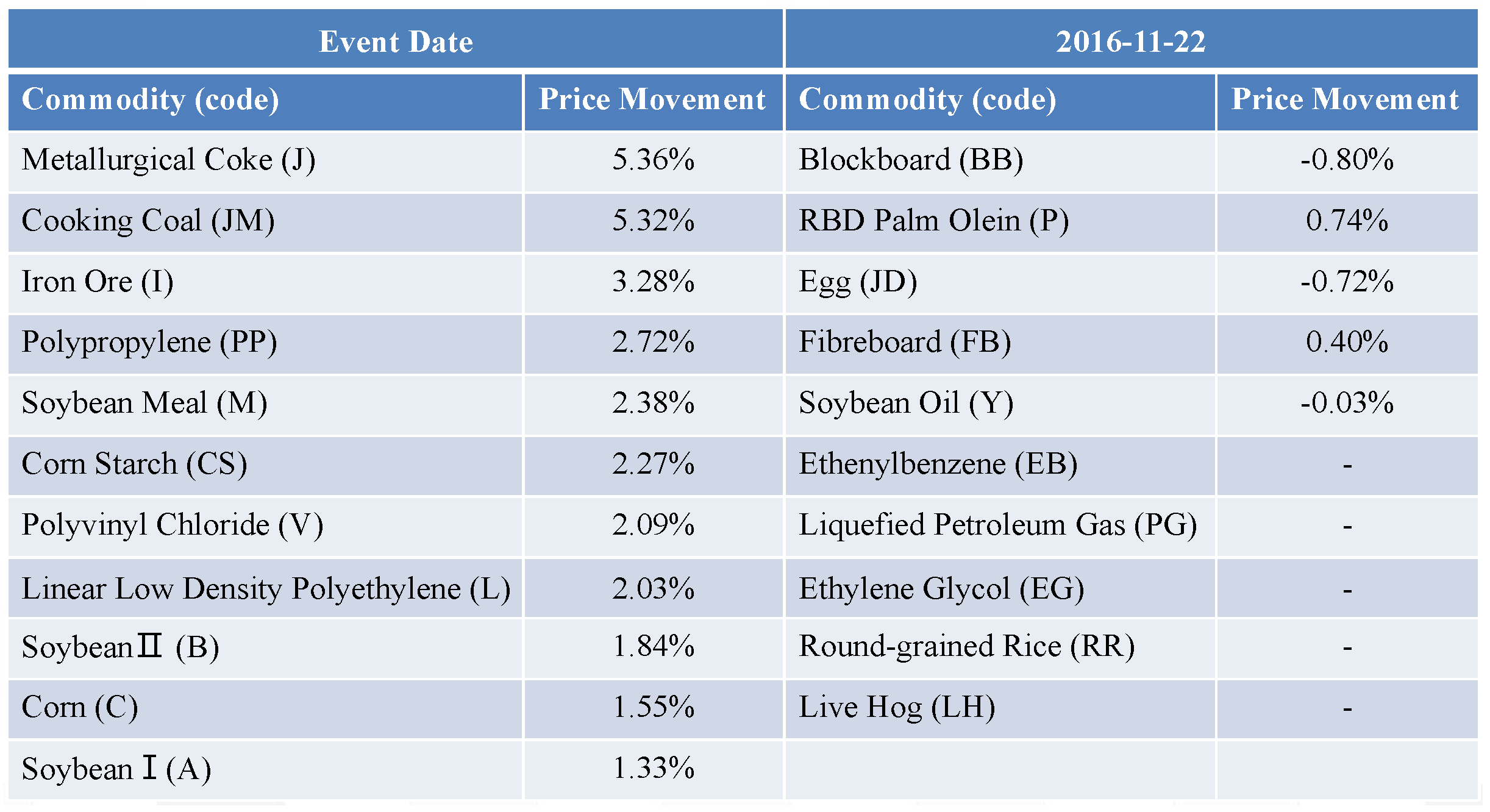
2.1. Historical Extreme Events

An historical extreme event typically contains extreme price movements in one or more risk factors. In the commodity futures market, the risk factor concerned is the commodity futures price. Therefore, we assumed that if any commodities incurred extreme market movements, this was defined as an historical extreme event. Motivated by Wang et al. (2021), who defined the top 1% quantiles of the distribution of daily price movements as extreme price movements, we also applied this method to define extreme movement, but increased quantiles to 2%. The collection of historical extreme events was created by searching the DCE market over the period from 4 January 2016 to 31 December 2021. An example of historical extreme events is shown in Figure 1, in which the event’s date was 22 November 2016. There were five commodities that exist today but had not yet been listed at the time of the event: Ethenylbenzene, Liquefied Petroleum Gas, Ethylene Glycol, Round-grained Rice, and Live Hog. Notably, for commodity futures, there is usually a series of contracts with different delivery months, in which the one with a predominant proportion of trading volume is referred to as the dominant contract. Reducing the model’s dependent variables can greatly decrease the modeling complexity. Hence, only the dominant contract, the most representative one, was considered in this work for each commodity future.

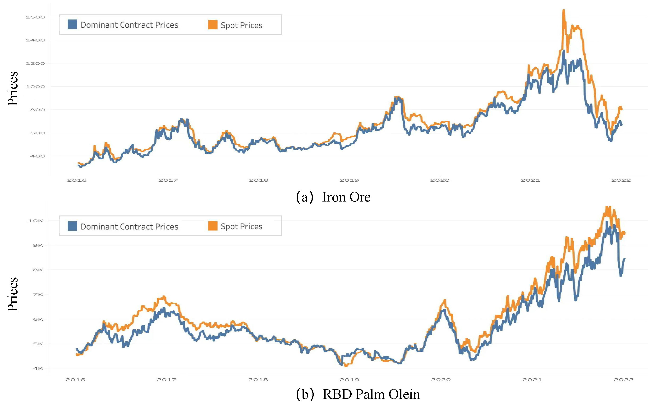
2.2. Multi-View Information

We sought multi-view information to provide task-related and discriminative features to input into the proposed model. It is well known that there are interrelations of different degrees among all commodities’ prices. Generally speaking, the commodity futures in the supply chain upstream and downstream tend to move up and down together, for example, SoybeanI and Soybean Meal. Thus, the prices of all the listed commodities in an historical extreme event are important to regress the unlisted commodity futures In addition, we also collected spot prices, the composite commodity index, and trading months. There were several motivations for such a design. First of all, it is common sense that commodity futures and spot prices usually have a similar tendency in practice, as shown in Figure 2.

Such similarity provides a significant feature for the inferring of decisions. Secondly, the composite commodity index is an index for a group of commodity prices, which usually reveals the directional movement of the overall group. For example, the commodities of DCE’s agricultural commodity group may collaboratively change because of factors such as weather, market, etc. This information is helpful in decision-making in regard to the potential direction of the commodity’s price movement. Thirdly, price movements of commodities, especially agricultural commodities, are closely related to the seasons, resulting in seasonal characteristics, to some extent. Thus, knowing the trading month in an event may provide potential information about seasonal characteristics.

A system was set up to gather multi-view information from different sources, including futures and spot markets2. Thus, given an historical extreme event, based on multi-view information, a feature vector $x\left(v\right)$ for a certain commodity v, can be defined as:

$$x\left(v\right)=[M_{fut},M_{spot},M_{group},D_{trade}],$$

(1)

where, $M_{fut}$, $M_{spot}$, and $M_{group}$ are price movements of commodity futures, spot, and composite commodity index, respectively, and $D_{trade}$ is a one-hot code representing trading month. The price movement for futures, spot, and composite commodity index, are, respectively, calculated by the following equation:

$$M=\frac{p_t-p_{t-1}}{p_{t-1}},$$

(2)

where, $p_t$ and $p_{t-1}$ denote prices for two consecutive days.

3. Method

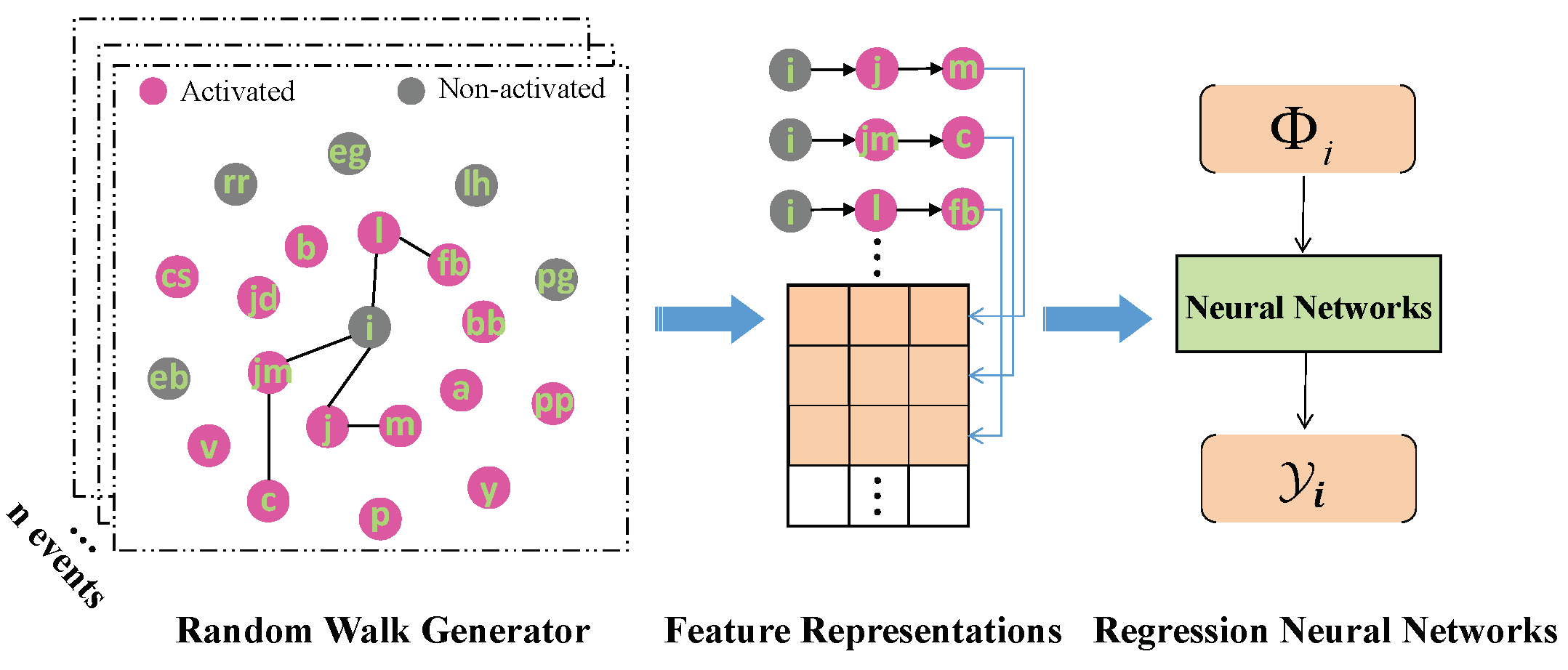
3.1. Approach Overview

We depict an overview of RCML in Figure 3. An event is represented by a graphic Wang et al. (2022) structure where all nodes denote various commodities, including listed and non-listed commodities, respectively named activated nodes and non-activated nodes.

Given an undirected graph, $G=(V,E,X,Y)$, where $V=\{v_1,v_2,...,v_m\}$ denote the set of nodes; $E\subseteq V\times V$ are edges among all nodes; $X=\{x\left(v_1\right),x\left(v_2\right),...,x\left(v_m\right)\}\in {\mathbb{R}}^{m\times \pi }$ is a set of feature vectors of all the nodes and $\pi$ is the dimension of the feature vector; $Y=\{y\left(v_1\right),y\left(v_2\right),...,y\left(v_m\right)\}\in {\mathbb{R}}^{m\times 1}$ is the set of labels which represent price movements of all the commodity futures. The unlisted commodities have no price movements, and, here, we set the labels of non-activated nodes as 0.

RCML consists of two main components, including a random walk generator Aldous and Fill (2002) and a Neural Network regressor. For the training phase, we trained the RCML model for each node. Take node $v_i$, for example, the random walk generator takes a set of graphs $\{G_1,G_2,...,G_n\}$ and generated massive feature representations. Then, these feature representations and corresponding labels are fed into the Neural Network’s regressor to train all the network’s parameters. In the testing phase, the result of node $v_i$ is generated by averaging the regressing results of all the feature representations. Figure 3 shows an example of the training process for the commodity Iron ore (code i). The details of the random walk generator and the Neural Networks regressor are, respectively, introduced in Section 3.2 and Section 3.3. The whole training process of ICML is depicted in Algorithm 1.

3.2. Random Walk Generator

The random walk generator aims to generate numerous random walks for a certain node from a set of graphs $\{G_1,G_2,...,G_n\}$. In terms of these walks, corresponding feature representations are produced for regressing the price movement. A random walk is known as a random process Xia et al. (2019). It describes a path consisting of a secession of random steps in the graph structure. Particularly, given a completely connected graph G, we can build d walks for node $v_i$. Each walk starts from node $v_i$ and the whole walk is denoted by $W_{v_i}$, including nodes ${\mathcal{W}}_{v_i}^1,{\mathcal{W}}_{v_i}^2,...,{\mathcal{W}}_{v_i}^k,...$, where $k=1,...,l$ and ${\mathcal{W}}_{v_i}^k$ is a random variable describing the position of a random walk after k steps and chosen from the immediate neighbors of a node ${\mathcal{W}}_{v_i}^{k-1}$, but excluding non-activated nodes. If the walk locates at the node i, the single step transition probability refers to the probability that the random walk can move to node j after the next step. It is represented as $Q_{ij}$ and can be denoted as:

$$Q_{ij}=Pr({\mathcal{W}}_{v_i}^k=j|{\mathcal{W}}_{v_i}^{k-1}=i).$$

(3)

$a_{ij}$ denotes the weight of the edge from the node i to the node j. Then, the transition probability from node i to node j can be defined as:

$$Q_{ij}=\left\{\begin{array}{c}\hfill \frac{a_{ij}}{{\sum }_m{a}_{im}}\mathrm{if}\left(i,j\right)\in E,i\ne j\hfill \\ \hfill 0\mathrm{otherwise}\hfill \end{array}\right.,$$

(4)

where, $a_{ij}$ is a correlation measure and we compute this correlation measure by using Pearson’s Correlation Coefficient Benesty et al. (2009) between price movements of commodities i and j during the last D trading months. Motivated by Fuhrman (1997), D was set at 12 months in this work. The final transition probabilities are calculated by normalizing the sum of each row to 1. Depending on a random walk, the corresponding feature representation is created as follows:

$${\varphi }_{v_i}=[x\left({\mathcal{W}}_{v_i}^1\right),x\left({\mathcal{W}}_{v_i}^2\right),...,x\left({\mathcal{W}}_{v_i}^l\right)].$$

(5)

Algorithm 1: Training process of RCML model

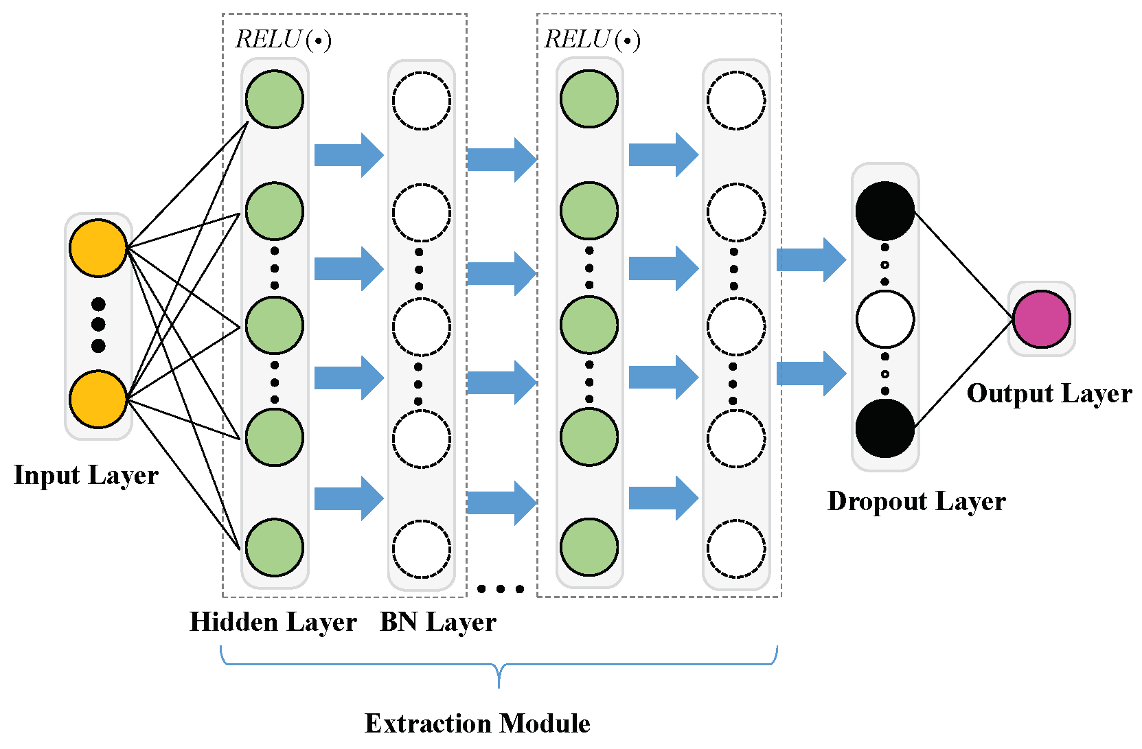
3.3. Neural Networks Regressor

A Neural Networks regressor was especially designed to regress reasonable price movement by generated feature representation ${\mathsf{\Theta }}^{*}$ for a certain node, and is presented in this section. Neural Networks Liu et al. (2021); Wang et al. (2020) are commonly viewed as a combination of interconnected linear processing elements, known as neurons, which obtain inputs and calculate outputs. Inspired by the human brain, Neural Networks mimic how biological neurons signal to one another. In general, Neural Networks are comprised of an input layer, one or more hidden layers, and an output layer, and each layer is distributed with neurons. The neurons of input and output layers correspond to the independent and dependent variables in specific tasks. For this task, they were feature representations and labels of a certain node. All neurons are connected between the layers with associated weights. For each neuron, based on these weights, all inputs are modified and then summed, obtaining the input. An activation function is usually adopted to map the node’s input to its corresponding output. The training process is aimed at maximizing the performance of the whole network through the optimization of the neurons’ weights by means of iterative adjustment of a performance function.

The proposed network architecture is shown in Figure 4, including an input layer, an extraction module, a dropout layer, and an output layer. The purpose of these NNs is to learn the optimal parameter set ${\mathsf{\Theta }}_{v_i}^{*}$ mapping ${\mathsf{\Phi }}_{v_i}$ to the label (price movement) ${\mathcal{Y}}_{v_i}$:

$${\mathsf{\Theta }}_{v_i}^{*}=\underset{\mathsf{\Theta }}{argmin}f({\mathsf{\Phi }}_{v_i},{\mathcal{Y}}_{v_i}).$$

(6)

The Extraction module contains three blocks, each composed of hidden and BN layers. The neurons of the hidden layer are successively decreased by half, and the starting hidden layer was set as the data dimension in this paper. For a hidden layer, the output of p-th neuron of k-th hidden layer can be expressed as:

$$ne{t}_p^k=g(\sum _{q=1}^Q{w}_{qp}^{k}ne{t}_q^{k-1}+a_p^k),$$

(7)

where, $w_{qp}^k$ is the associated weight between the q-th neuron in the $k-1$-th layer and the p-th neuron in the k-th layer; $a_p^k$ is a bias on the p-th neuron; $g(·)$ denotes an activation function. The choice of activation function3 is an important design for the hidden layer. There are three main types of activation functions: Rectified Linear Unit (ReLU) Agarap (2018), Sigmoid Marreiros et al. (2008), and Hyperbolic Karlik and Olgac (2011). ReLU was a more appropriate choice for our task than the other two functions because of its superior ability to address the saturation problem Lau and Lim (2017) and converge much faster. It has been popularly adopted in economics and financial applications Fabozzi et al. (2019). Its specific format can be represented as $g\left(x\right)=max(0,x)$. After the hidden layer, a batch normalization (BN) layer is employed to normalize the hidden layer’s outputs by re-centering and re-scaling. Using the BN layer can make the training process more stable and significantly enhance the network’s generalization ability. The details of BN layer are referred to in Santurkar et al. (2018). Following the Extraction module, a dropout layer with $p=0.5$ is added to reduce overfitting by omitting each neuron with probability Labach et al. (2019). A final hidden layer aims to transfer high-dimensional features into the one-dimensional label.

The training procedure includes forward propagation and back propagation stages. In the forward propagation stage, the proposed network calculates the regressed results of training samples. In the back propagation stage, according to the error between regressed results and real labels, all the weights and biases are updated by the Adam Kingma and Ba (2014) algorithm. Adam is an adaptive variation of the gradient descent algorithm, which was designed specifically for training Neural Networks. Specifically, this method computes individual adaptive learning rates for each weight of the Neural Network from estimates of the first and second moments of the gradients. This computationally efficient property greatly facilitated the training process for large amounts of feature representations in this work.

Forward and back propagation stages were repeatedly executed until the Mean Absolute Error (MAE) between the regressed and real labels was the minimum or the maximum number of repeats reached. Particularly, MAE was calculated as the sum of absolute errors divided by sample size $n^{\prime }d$:

$$MAE=\frac{{\sum }_s^{n^{\prime }d}\left|regression\left({\varphi }_s\right)-real\left({\varphi }_s\right)\right|}{n^{\prime }d},$$

(8)

where, $regression\left({\varphi }_s\right)$ is the regressed result and $real\left({\varphi }_s\right)$ is the real label.

4. Experiments

4.1. Dataset

According to the definition given in Section 2.1, we collected 296 historical extreme events in the DCE market from 4 January 2016 to 31 December 2021. There are currently 21 listed commodities, including 12 commodities from the agricultural group and 9 commodities from the industrial group. Specifically, commodities of the agricultural group are Corn (C), Corn Starch (CS), SoybeanI (A), SoybeanII (B), Soybean Meal (M), Soybean Oil (Y), RBD Palm Olein (P), Fibreboard (FB), Blockboard (BB), Egg (JD), Round-grained Rice (RR), Live Hog (LH). Commodities in the agricultural group are Linear Low Density Polyethylene (L), Polyvinyl Chloride (V), Polypropylene (PP), Ethylene Glycol (EG), Ethenylbenzene (EB), Metallurgical coke (J), Cooking coal (JM), Iron Ore (I), Liquefied Petroleum Gas (PG). The bracketed text indicates trading code. We trained the inferring model for each commodity using the proposed RCML.

4.2. Model Setup

Our code was written in Python, based on Pytorch. For the random walk generator, the length of the walk and the number of walks were set as 6 and 2000, respectively. We adopted batch size 64 for 1000 epochs for the Neural Networks regressor and set an initial learning rate of 5.0 × ${10}^{-6}$. The learning rate automatically decreased by a factor of 0.7 when the loss stopped improving after 3 epochs. In addition, we set up an early stop mechanism, whereby training stopped when a monitored quantity stopped improving, even if the epoch had not reached 1000.

4.3. Back Testing

Of the commodities, 16 were listed before 4 January 2016, and, thus, had price movements (real labels) in all the events. The remaining five commodities, Ethylene Glycol, Round-grained Rice, Ethenylbenzene, Liquefied Petroleum Gas, and Live Hog were exceptions. In this section, we adopted back testing to validate RCML’s inferring error on the 16 commodities, including Soybean Meal, SoybeanI, etc. Back testing involves applying a predictive model to historical data to determine its accuracy. It is usually used to test and compare the viability of trading strategies in economics Zhang and Nadarajah (2018). For this work, back testing was introduced to compare the errors between price movements (real labels) and regression results in randomly selected historical extreme events. The training, testing, and validating events were randomly partitioned following the proportion 6/2/2. For each commodity, we performed a 10-folds cross validation to evaluate the inferring performance. The total inferring error was calculated as the average of the 10-folds cross validation.

A baseline was constructed by replacing the Neural Networks with Linear Regression (LR) Montgomery et al. (2021), which was helpful to evaluate the regression ability of the proposed regression network and to validate the discriminative power of the feature representations. The Linear Regression was implemented using the sci-kit-learn library, which already provides excellent default parameters.

Table 1. The inferring results of averaged MAE (%) of RCML and baseline.

Commodity	RCML	Baseline	Commodity	RCML	Baseline
C	0.64%	0.72%	PP	0.83%	0.80%
CS	0.80%	0.89%	J	0.97%	1.21%
A	0.89%	0.94%	Y	0.56%	0.59%
B	0.71%	0.94%	P	0.59%	0.54%
M	0.56%	0.58%	FB	0.99%	1.11%
I	0.95%	1.06%	BB	0.45%	0.47%
JD	1.02%	1.21%	JM	1.38%	1.65%
L	0.90%	1.01%	V	0.93%	0.82%

shows the MAE errors of the RCML and the baseline for different commodities. From these results, we observe that the RCML and the baseline achieved superior performances on these commodities. Most of the errors were less than 1%. This indicated that the feature representations, comprised of multi-view information and sampled by the random walk generator, offered significant discriminative information for the learning processes of the proposed Neural Networks regressor and LR. Furthermore, these results also suggest that, compared with the baseline, the proposed Neural Networks regressor had better fitting capability on most of the commodities. In the study presented, we used the same parameters for training the RCML models on all the commodities. Thus, it was hard to find a set of parameters that was superior for all the commodities. For the PP, P, and V commodities, the RCML performed slightly worse than the baseline model, which might have been because of the model’s improper parameters. This motivated us to improve the RCML model with flexible parameter selection for specific commodities in future study. Overall, these experimental results provide evidence that RCML can infer rational price movements for commodities when they were not listed in historical extreme events.

4.4. Hypothesis Testing

In the previous section, we discussed RCML’s performance in terms of comparing the errors between inference results and real labels for 16 commodities. The remaining 5 commodities, Ethylene Glycol, Round-grained Rice, Ethenylbenzene, Liquefied Petroleum Gas, and Live Hog, were, respectively, listed on the following dates: 10 December 2018, 16 August 2019, 26 September 2019, 30 March 2020, and 8 January 2021. Thus, they had no label information for events between 4 January 2016 and their respective listing dates. To assess RCML’s inferring performance without the use of label information, Kolmogorov–Smirnov (KS) Hassani and Silva (2015) testing, a well-known hypothesis testing method, was used to check whether the results referred to and the observed samples originated from the same distribution.

It must be pointed out that the time since the Live Hog commodity was listed on the DCE market is very short, so its training data size was too limited to train the RCML model. Thus, the experiments in this section only focused on Ethylene Glycol, Round-grained Rice, Ethenylbenzene, and Liquefied Petroleum Gas. For each of these, we respectively selected the historical extreme events without labels and generated inferred results. Then, we collected the observed samples from the historical extreme events where these commodities were already listed. Finally, the inferred results were compared to the observed samples using KS statistics, which were compared to a threshold to make a decision. The KS testing was implemented using the Python SciPy.stats.ks_2samp library, that automatically displays statistic D and p-values. If the statistic D was small, or the p-value exceeded the threshold (p-value = 0.05 in this work), we could not reject the null hypothesis that the inferred results and observed samples originated from the same distribution. In other words, if p-value>0.05, we believed that they were drawn from identical distributions, and the referring results of the proposed model were reasonable for unlisted commodities in the historical events. The statistical results of KS testing are listed in

Table 2. KS testing results.

Commodity	Inferring Results Size	Observed Sample Size	p-Value	Statistic D	Decision
EB	139	157	0.226	0.1185	Cannot Reject
PG	162	134	0.222	0.1194	Cannot Reject
EG	134	162	0.033	0.163	Rejected
RR	136	160	0.036	0.162	Rejected

.

Table 3. A representative example of historical extreme events.

Date			22 November 2016
Commodity	Price Movement	Product	Price Movement	Commodity	Price Movement
C	1.55%	Y	−0.03%	V	2.09%
CS	2.27%	P	0.74%	I	3.28%
A	1.33%	FB	0.40%	EB	3.32%
B	1.84%	BB	−0.80%	EG	−0.17%
M	2.38%	JD	−0.72%	PG	−1.28%
PP	2.72%	L	2.03%	RR	−0.1%
J	5.36%	JM	5.32%	LH	-

further shows an historical extreme event, in which the results of EB, RR, PG, EG are inferred by RCML.

From these results, we observe that the p-value of EB and PG were higher than the threshold, so we accepted the null hypothesis that the two data sets were drawn from the identical distribution. To some extent, this indicated that the inferred results conformed to reality for EB and PG. However, for EG and RR, the p-values were less than 0.05, and the distributions of the inferred results and real samples were considered to be different. Thus, we tended to believe that the inferred results for these two commodities were unreasonable. The reasons for these failures might have been a big gap between the price movements of commodity futures and spots in the training data, or some unsuitable model parameters leading to poor generalization performance, or something else, which will be explored in our future work.

5. Conclusions

It is well known that stress testing has long been a part of the risk management toolkit. Historical scenario simulation, the most representative method for performing stress testing, refers to the revaluation of historical adverse market events on a financial institution’s current portfolios. This method usually relies on human hypothesis when the currently cleared products did not exist in an historical event. Therefore, this paper aimed to use ML technologies to solve the lack of price information in unlisted commodity futures in an historical scenario simulation. The presented method effectively combines Random Walk and Neural Network, and is named RCML. The RCML method improves and automates historical scenario simulations by regressing reasonable price information for unlisted commodity futures, avoiding total dependence on subjective hypothesis. To ensure effective RCML training, we further explored the commodity’s feature vector derived from multi-view information and collected a set of historical extreme events. Extensive experiments validated the RCML’s performance by using back testing and hypothesis testing. When comparing the real labels in back testing, the regressing errors for most of the commodities were less than 1%, indicating that RCML makes accurate regression decisions. In the hypothesis testing experiments, checking the distribution similarity between the regressing results and the observed samples showed that RCML inferred relatively reasonable price movement for unlisted commodities. We also experienced some failures. The most important one was that the RCML’s inferences for a few commodities seemed to have poor generalization ability (details can be referred to in Section 4.4). In future works, we will explore the factors and corresponding solutions.

References

1. Agarap, Abien Fred. 2018. Deep learning using rectified linear units (relu). arXiv arXiv:1803.08375. [Google Scholar]
2. Aldous, David, and James Fill. 2002. Reversible Markov Chains and Random Walks on Graphs. Unfinished Monograph, Recompiled 2014. Available online: http://www.stat.berkeley.edu/~aldous/RWG/book.html (accessed on 16 September 2022).
3. Benesty, Jacob, Jingdong Chen, Yiteng Huang, and Israel Cohen. 2009. Pearson correlation coefficient. In Noise Reduction in Speech Processing. Berlin/Heidelberg: Springer, pp. 1–4. [Google Scholar]
4. Blaschke, Winfrid, Matthew T. Jones, Giovanni Majnoni, and Maria Soledad Martinez Peria. 2001. Stress Testing of Financial Systems: An Overview of Issues, Methodologies, and FSAP Experiences. IMF Working Papers 2001/088. Washington, DC: International Monetary Fund. [Google Scholar]
5. Duch, Włodzisław, and Norbert Jankowski. 1999. Survey of neural transfer functions. Neural Computing Surveys 2: 163–212. [Google Scholar]
6. EUR. 2017. Draft Guidelines on Institution’s Stress Testing, (Consultation Paper). Technical Report, European Banking Authority. Available online: https://www.eba.europa.eu (accessed on 12 June 2022).
7. Fabozzi, Frank J., Hasan Fallahgoul, Vincentius Franstianto, and Gregoire Loeper. 2019. Towards Explaining Deep Learning: Asymptotic Properties of Relu FFN Sieve Estimators. Available online: https://ssrn.com/abstract=3499324 (accessed on 12 June 2022).
8. Fuhrman, Roger D. 1997. Stress testing portfolios to measure the risk faced by futures clearinghouses. Paper presented at NCR-134 Conference on Applied Commodity Forecasting and Risk Management, Chicago, IL, USA, April 20; pp. 401–11. [Google Scholar]
9. Gogas, Periklis, Theophilos Papadimitriou, and Anna Agrapetidou. 2018. Forecasting bank failures and stress testing: A machine learning approach. International Journal of Forecasting 34: 440–55. [Google Scholar] [CrossRef]
10. Hassani, Hossein, and Emmanuel Sirimal Silva. 2015. A kolmogorov-smirnov based test for comparing the predictive accuracy of two sets of forecasts. Econometrics 3: 590–609. [Google Scholar] [CrossRef]
11. Huang, Xin, Hao Zhou, and Haibin Zhu. 2009. A framework for assessing the systemic risk of major financial institutions. Journal of Banking & Finance 33: 2036–49. [Google Scholar]
12. Ivanov, Alexei, and Giuseppe Riccardi. 2023. Meng wang, rethinking data-free quantization as a zero-sum game. Paper presented at AAAI Conference on Artificial Intelligence, Washington, DC, USA, February 7–14. [Google Scholar]
13. Karlik, Bekir, and A. Vehbi Olgac. 2011. Performance analysis of various activation functions in generalized mlp architectures of neural networks. International Journal of Artificial Intelligence and Expert Systems 1: 111–22. [Google Scholar]
14. Kingma, Diederik P., and Jimmy Ba. 2014. Adam: A method for stochastic optimization. arXiv arXiv:1412.6980. [Google Scholar]
15. Kristjanpoller, Werner, and Marcel C. Minutolo. 2015. Gold price volatility: A forecasting approach using the artificial neural network–garch model. Expert Systems with Applications 42: 7245–51. [Google Scholar] [CrossRef]
16. Kulkar, Siddhivinayak, and Imad Haidar. 2009. Forecasting model for crude oil price using artificial neural networks and commodity future prices. International Journal of Computer Science and Information Security 2: 81–88. [Google Scholar]
17. Labach, Alex, Hojjat Salehinejad, and Shahrokh Valaee. 2019. Survey of dropout methods for deep neural networks. arXiv arXiv:1904.13310. [Google Scholar]
18. Lau, Mian Mian, and King Hann Lim. 2017. Investigation of activation functions in deep belief network. Paper presented at 2017 2nd International Conference on Control and Robotics Engineering (ICCRE), Bangkok, Thailand, April 1–3; pp. 201–6. [Google Scholar]
19. Liu, Caifeng, Lin Feng, Guochao Liu, Huibing Wang, and Shenglan Liu. 2021. Bottom-up broadcast neural network for music genre classification. Multimedia Tools and Applications 80: 7313–31. [Google Scholar] [CrossRef]
20. Marreiros, André C., Jean Daunizeau, Stefan J. Kiebel, and Karl J. Friston. 2008. Population dynamics: Variance and the sigmoid activation function. Neuroimage 42: 147–57. [Google Scholar] [CrossRef] [PubMed]
21. Montgomery, Douglas C., Elizabeth A. Peck, and G. Geoffrey Vining. 2021. Introduction to Linear Regression Analysis. Hoboken: John Wiley & Sons. [Google Scholar]
22. Mudry, Pierre-Antoine, and Florentina Paraschiv. 2016. Stress-testing for portfolios of commodity futures with extreme value theory and copula functions. In Computational Management Science. Berlin/Heidelberg: Springer, pp. 17–22. [Google Scholar]
23. Nas. 2014. Nasdaq Clearing Ab Ccar Model Instructions. Technical Report, Nasdaq Clearing’s Risk Management Department. Available online: https://www.nasdaq.com/docs/CCaR-Model-Instructions-171110.pdf (accessed on 3 June 2022).
24. Petropoulos, Anastasios, Vassilis Siakoulis, Konstantinos P. Panousis, Theodoros Christophides, and Sotirios Chatzis. 2020. A deep learning approach for dynamic balance sheet stress testing. arXiv arXiv:2009.11075. [Google Scholar]
25. PSS. 2009. Principles for Sound Stress Testing Practices and Supervision. Technical Report, Basel Committee on Banking Supervision. Available online: https://www.bis.org/publ/bcbs155.htm (accessed on 1 July 2022).
26. PFM. 2017. Principles for Financial Market Infrastructures. Technical Report, International Organization of Securities Commission & Committee on Payments and Market Infrastructures. Available online: https://www.bis.org/cpmi/info_pfmi.htm (accessed on 1 July 2022).
27. RMG. 1999. Risk Management: A Practical Guide. Technical Report, RiskMetrics Group. Available online: https://www.msci.com/documents/10199/3c2dcea9-97be-4fb4-befe-a03b75c885aa (accessed on 1 July 2022).
28. Santurkar, Shibani, Dimitris Tsipras, Andrew Ilyas, and Aleksander Madry. 2018. How does batch normalization help optimization? arXiv arXiv:1805.11604. [Google Scholar]
29. Wang, Huibing, Guangqi Jiang, Jinjia Peng, Ruoxi Deng, and Xianping Fu. 2022. Towards adaptive consensus graph: Multi-view clustering via graph collaboration. IEEE Transactions on Multimedia 1–13. [Google Scholar] [CrossRef]
30. Wang, Huibing, Jinjia Peng, Dongyan Chen, Guangqi Jiang, Tongtong Zhao, and Xianping Fu. 2020. Attribute-guided feature learning network for vehicle reidentification. IEEE MultiMedia 27: 112–21. [Google Scholar] [CrossRef]
31. Wang, Lu, Feng Ma, Tianjiao Niu, and Chao Liang. 2021. The importance of extreme shock: Examining the effect of investor sentiment on the crude oil futures market. Energy Economics 99: 105319. [Google Scholar] [CrossRef]
32. Wang, Yang. 2021. Survey on deep multi-modal data analytics: Collaboration, rivalry, and fusion. ACM Transactions on Multimedia Computing, Communications, and Applications (TOMM) 17: 1–25. [Google Scholar] [CrossRef]
33. Wang, Yang, Jinjia Peng, Huibing Wang, and Meng Wang. 2022. Progressive learning with multi-scale attention network for cross-domain vehicle re-identification. Science China Information Sciences 65: 1–15. [Google Scholar] [CrossRef]
34. Worrachartdatchai, Usanee, and Pitikhate Sooraksa. 2007. Credit scoring using least squares support vector machine based on data of thai financial institutions. Paper presented at The 9th International Conference on Advanced Communication Technology, Phoenix Park, Republic of Korea, February 12–14; Volume 3, pp. 2067–70. [Google Scholar]
35. Xia, Feng, Jiaying Liu, Hansong Nie, Yonghao Fu, Liangtian Wan, and Xiangjie Kong. 2019. Random walks: A review of algorithms and applications. IEEE Transactions on Emerging Topics in Computational Intelligence 4: 95–107. [Google Scholar] [CrossRef]
36. Zhang, Heng-Guo, Chi-Wei Su, Yan Song, Shuqi Qiu, Ran Xiao, and Fei Su. 2017. Calculating value-at-risk for high-dimensional time series using a nonlinear random mapping model. Economic Modelling 67: 355–67. [Google Scholar] [CrossRef]
37. Zhang, Y., and S. Nadarajah. 2018. A review of backtesting for value at risk. Communications in Statistics-Theory and Methods 47: 3616–39. [Google Scholar] [CrossRef]
Figure 1. An example of an historical extreme event (‘-’ denotes the unlisted commodity).
Jrfm 16 00285 g001
Figure 2. The price series of dominant contracts and spots of DCE’s Iron Ore and DCE’s RBD Palm Olein for the period from 4 January 2016 to 31 December 2021.1
Jrfm 16 00285 g002
Figure 3. Overview of the proposed approach HRW.
Jrfm 16 00285 g003
Figure 4. The architecture of the proposed regression Neural Networks.
Jrfm 16 00285 g004