Article

Precious Metals Comovements in Turbulent Times: COVID-19 and the Ukrainian Conflict

by
Antonis A. Michis
1,2
1
Central Bank of Cyprus, Nicosia 1076, Cyprus
2
Department of Business Administration, School of Business and Law, Frederick University, Nicosia 1036, Cyprus
J. Risk Financial Manag. 2023, 16(5), 280; https://doi.org/10.3390/jrfm16050280
Submission received: 28 March 2023 / Revised: 12 May 2023 / Accepted: 17 May 2023 / Published: 20 May 2023
(This article belongs to the Special Issue Comovement of International Financial Markets II)

Abstract

:
We examined the evolution of cross-market linkages between four major precious metals and US stock returns, before (Phase I) and after (Phase II) the COVID-19 outbreak. Phase II was also extended to encompass the Ukrainian conflict, which prolonged the period of uncertainty in financial markets. Due to the increase in volatility observed in Phase II, we used a heteroskedasticity-adjusted correlation coefficient to examine the evolution of correlation changes since the COVID-19 outbreak. We also propose a relevant dissimilarity measure in multidimensional scaling analysis that can be used for depicting associations between financial returns in turbulent times. Our results suggest that (i) the correlation levels of gold, silver, platinum, and palladium returns with US stock returns have not changed substantially since the COVID-19 outbreak, and (ii) all precious metal returns exhibit movements that are less synchronized with US stock returns, with palladium and gold being the least synchronized.

1. Introduction

In addition to exhibiting good diversification properties in the context of investment portfolios (Conover et al. 2009), precious metals are frequently considered to possess good safe haven and hedging properties during periods of financial distress (Baur and Lucey 2010). As a result of these unique characteristics, precious metals received renewed interest from equity investors with the outbreak of the COVID-19 pandemic, since a “flight to quality” effect was observed in response to the increased volatility in equity markets. Several recent studies have provided empirical evidence for this effect, particularly in the case of gold (see, for example, the studies by Akhtaruzzaman et al. 2021; Lahiani et al. 2021).
A central theme in these studies (reviewed in Section 2) is the derivation of correlation estimates between precious metals and equity returns, using insights from the financial contagion (Corbet et al. 2020) and mean-variance portfolio (Ji et al. 2020) frameworks in the finance literature. Such correlation estimates are frequently used by investors to better understand the associations and comovements among the various asset classes, when considering the allocation of their financial resources in the context of investment portfolios. For example, in a recent study of Asian markets, Yousaf et al. (2021) found that the optimal weights in portfolios that combine stocks with gold have changed since the outbreak of the COVID-19 pandemic.
This study contributes to the existing literature by demonstrating that during the recent turbulent period of increased stock market volatility that began with the COVID-19 pandemic (Kumar and Padakandla 2022), the standard correlation coefficient estimates between precious metals and stock market returns become biased and unreliable. This heteroscedasticity bias can be corrected using the unconditional correlation coefficient proposed by Forbes and Rigobon (2002) in the context of the financial contagion literature. We also propose a multidimensional scaling analysis (MSA) procedure, using a dissimilarity measure based on the unconditional correlation coefficient. It can be used by investors to better understand the similarities (or differences) between precious metals and stock market returns.
The heteroscedasticity bias in the correlation estimates between financial returns during turbulent times exists because correlation coefficients are conditional on market volatility. Consequently, when heteroscedasticity exists in the financial returns of an asset (e.g., due to a shock), the cross market correlation estimates of other return series with this asset will be inflated, even though the underlying cross-market linkages between the two series have not changed.
In finance, this correlation bias is most commonly encountered in the financial contagion literature, when estimating cross-country market linkages after a shock (Loretan and English 2000) and in the estimation of intra-market correlations between stocks and bonds during periods of increased market volatility (Ronn 1998). Forbes and Rigobon (2002) provided a formal proof of this bias using stochastic variables that represent stock market returns. The authors also provided a method for adjusting this bias, which we discuss in Section 3.
We demonstrate our proposed method using the financial returns for four precious metals (gold, palladium, platinum, and silver) and the US stock market returns, over the period from February 2010 to January 2023. This period can be divided into two phases: before (Phase I) and after (Phase II) the COVID-19 outbreak, with the second phase also extending into the Ukrainian conflict. The COVID-19 cluster in China was first announced on 31 December 2019, and the transition to an endemic status for COVID-19 was first announced for the USA on 17 February 2022, in California.
On 24 February 2022, Russian President Vladimir Putin announced a “special military operation” in Ukraine that marked the beginning of the Ukrainian conflict, and which has extended beyond January 2023, which is the latest period covered by the dataset used for this study. We therefore defined the two phases in our study as follows: Phase I (the stable period)—from February 2010 to December 2019; and Phase II (the turbulent period)—from January 2020 to January 2023, covering both the COVID-19 pandemic and the Ukrainian conflict.
Our results suggest an increase in stock market volatility during Phase II that biases correlation estimates, providing, therefore, misleading inferences to investors. When correlation estimates are corrected, the correlation levels between US stock returns and precious metal returns were not found to have changed substantially. In addition, US stock returns were found to be less synchronized with precious metal returns, suggesting that precious metals constitute useful assets for diversification purposes. Gold, silver, and platinum returns exhibited more similar movements between them, while palladium exhibited the highest level of dissimilarity from all other assets.
The rest of this article is organized as follows: Section 2 reviews the relevant literature concerning the use of precious metals as investment assets, as well as the use of correlation coefficients in financial applications. Section 3 presents the unconditional correlation coefficient that corrects the heteroscedasticity bias in standard correlation estimates and the proposed MSA methodology for depicting the synchronization of comovements between financial returns. Section 4 empirically demonstrates the importance of correcting the heteroscedasticity bias in correlation estimates and investigates the comovements between different assets during the two phases. Section 5 summarizes the main findings of the study.

2. Literature Review

Precious metals, predominantly gold, are frequently considered as alternative investment assets with good diversification, hedging or safe haven properties; see, for example, the studies by Skiadopoulos (2012); Mensi et al. (2013); Michis (2014, 2019, 2022); Lucey and Li (2015). According to Baur and Lucey (2010), a diversifier exhibits non-perfect positive correlation with other assets (or a portfolio of assets), on average, while an effective hedge exhibits zero or negative correlation with other assets, on average. The safe haven property requires zero or negative correlation during times of financial distress.
The outbreak of the COVID-19 pandemic increased the level of uncertainty in the financial markets, which, in turn, caused renewed interest from professional investors in the aforementioned properties of precious metals. This “flight to quality” effect increased the prices of some precious metals at a time when sharp declines were recorded in all major stock market indices, most prominently in the USA (Lahiani et al. 2021). These developments have been the subject of several recent empirical studies in the finance literature that re-examined the safe haven properties of precious metals (Ji et al. 2020; Akhtaruzzaman et al. 2021; Salisu et al. 2021; Yousaf et al. 2021; Chemkha et al. 2021). Nearly all of these studies provide evidence for the safe haven properties of gold during the COVID-19 era, with some studies also providing similar results for platinum and palladium (Lahiani et al. 2021), as well as the hedging effectiveness of silver (Salisu et al. 2021).
With respect to the methodologies, various methods have been proposed in the literature for examining the relationships between various asset classes and precious metals. For example, Lahiani et al. (2021) used a nonlinear autoregressive distributed lag model to examine the short-run and long-run relationships between the S&P 500 index and precious metals, while Michis (2021) employed a multiscale partial correlation clustering method to examine the comovements between precious metal futures, energy futures, and stock returns. Other methodologies employed include dynamic conditional correlation GARCH models (Peng 2020), conditional VaR and copula methods (Uddin et al. 2020), VARMA-GARCH models (Salisu et al. 2021), time-varying parameter VAR models (Bouri et al. 2021), connectedness indices based on VAR models (Bahloul and Khemakhem 2021), and time-varying Granger causality tests (Gharib et al. 2021).
In this study, an MSA is proposed for investigating the comovements of precious metals with US stock returns. Central to this analysis is the use of a distance metric (or dissimilarity measure) based on the unconditional correlation coefficient proposed by Forbes and Rigobon (2002). Multivariate analysis and alternative correlation methods have also been used by other authors in the literature for examining the associations between various assets classes. Examples include the Pearson correlation coefficient (Geertsema and Lu 2020), time-varying correlation methods (Chiang et al. 2007), partial-correlation coefficients (Kenett et al. 2015; Jung and Chang 2016), Fisher correlation (Krishnan et al. 2009), dynamic conditional correlation (Engle and Colacito 2006), partial-distance correlation (Creamer and Lee 2019), de-trended cross-correlation (Wątorek et al. 2019), and the multiscale partial-correlation coefficient (Michis 2022).
Regarding the use of MSA for the analysis of financial and economic time series, existing research has relied mainly on Euclidean (Machado et al. 2011; Cox 2013) and spectral (Fourier- or wavelet-based) distance metrics (Camacho et al. 2006; Aguiar-Conraria and Soares 2011; Aguiar-Conraria et al. 2013). Our study is the first to use a time-series distance metric based on a heteroscedasticity-adjusted correlation coefficient.

3. Methodology

3.1. Unconditional Correlation Coefficient

Considering the following relationship between two stochastic processes,  y t  and  x t ; in the context of the current study, these represent financial returns:
y t = a + β x t + ε t
The residuals are assumed to have the following standard properties:
E [ ε t ] = 0 ,   E [ ε t 2 ] = c <   and   E [ x t ε t ] = 0 .
Supposing, next, that the sample of time series observations can be divided into two groups, where the variance in the first group ( σ x x l o w ) is lower from the variance in the second group ( σ x x h i g h ); in the context of the current study, the first group is the period prior to the COVID-19 pandemic (Phase I) and the second group is the period after the COVID-19 pandemic, which extends into the Ukrainian conflict (Phase II).
By assumption,  σ x x h i g h > σ x x l o w  and the OLS coefficient estimates are consistent for both groups,  β h i g h = β l o w = β ; therefore, it can be shown that the following inequality holds:
σ x x σ y y h i g h > σ x x σ y y l o w
which implies a heteroscedasticity bias in the estimated correlation coefficient of the second period, conditional on the variance of  x  such that:
ρ h i g h = β σ x h i g h σ y h i g h > ρ l o w = β σ x l o w σ y l o w
Forbes and Rigobon (2002) proposed the following unconditional correlation coefficient that corrects the heteroscedasticity bias associated with the conditional correlation coefficient:
ρ = ρ * 1 + δ 1 ρ * 2 .
It can be observed that this correlation function incorporates the conditional correlation coefficient ( ρ * ) and the relative increase in the variance of  x t , which has the following form:
δ σ x x h σ x x l 1
The residual assumptions associated with Equation (1) suggest the absence of any endogeneity or omitted variable problems, such as feedback effects from asset class  y  to asset class  x  or any exogenous universal shocks. Nevertheless, Forbes and Rigobon (2002) also demonstrated that the adjustment in Equation (2) provides a good approximation to the unconditional correlation coefficient, even in cases where these problems exist, as long as three criteria for near-identification hold: (a) the change in market volatility is large; (b) the source of the increase in market volatility is clearly identified; and (c) the source of market volatility is included as one variable in the unconditional correlation estimate.
For the purposes of this study, we considered US stock market returns as the benchmark source financial variable in all applications of the unconditional correlation formula that satisfies the abovementioned criteria. In addition to its size and importance for the global financial system, existing research suggests that the demand for precious metals increases when: (i) there are negative developments in the prices of US stocks and investors prefer precious metals as safe haven assets, as in the study by Lahiani et al. (2021) for the COVID-19 era; and (ii) when there is a decline in the value of USD as a result of worsening macroeconomic conditions in the US economy, as studied by Joy (2011) and Reboredo (2013).

3.2. Multidimensional Scaling Analysis

In this subsection, we propose an MSA procedure for representing the associations between asset returns using two-dimensional spatial maps. MSA is a well-known multivariate analysis method for representing objects in low-dimensional spaces. These representations have the important property of preserving the similarities or dissimilarities between the objects in the actual data, in such a way that similar objects are located close to each other, while dissimilar objects are located further apart (Everitt and Hothorn 2011).
In this framework, the measurement of dissimilarity between the objects is an important consideration and various distance metrics have been proposed in the literature. In applied studies, the most commonly encountered dissimilarity measures are the Euclidean distance, the Mahalanobis distance, the Minkowski metric, and the correlation distance (Cox 2005). For the purposes of this study, we used a distance metric based on the unconditional correlation coefficient in Equation (2), as follows:
d ( ρ ) = 1 ρ = 1 ρ * 1 + δ 1 ρ * 2
Next, we incorporated this distance metric in classical MDS analysis, where the low-dimensional configuration of points (objects) is derived from a multistep algorithm as follows (Cox 2005):
Step 1:
Define an ( N × N ) matrix,  A , using the squared dissimilarities between all pairs of financial returns ( i , j ):
A = 1 2 d ρ i j 2
Step 2:
Form a positive semi-definite matrix,  B , with zero-sum rows and columns, using a centering matrix,  H , and where the center of coordinate points is set at the origin.
B = HAH   where   H = I N 1 11 T .
Step 3:
Derive the spectral decomposition of  B , where  Λ  and  V  are the matrices of ordered eigenvalues ( e 1 e 2 e N ) and normalized eigenvectors ( V i V i T = 1 ), respectively,
B = V Λ V T   where   Λ = d i a g ( e 1 , , e N )   and   V = ( V 1 , , V N ) .
Step 4:
Use the following coordinate matrix,  X , to represent the  N  objects in  N  dimensions:
X = V Λ 1 / 2 .
When the matrix  B  is of rank  k , it will have an equal number of positive eigenvalues. Therefore, ( N k ) zero eigenvalues can be excluded from its decomposition and the size of the coordinate matrix is reduced as follows:
X = V 1 Λ 1 1 / 2   where   Λ 1 = d i a g ( e 1 , , e k )   and   V 1 = ( V 1 , , V k ) .
The configuration in  X  is rotated to its principal axes such that the axes are orthogonal between them and the variation in the projected points on the axes follows a decreasing order. Therefore, in practice, it is common to represent objects using two-dimensional configurations, with only the first two columns in  X .
The objects are represented by points in the two-dimensional space and the distances between the points are analogous to the dissimilarities between the objects in the space of the actual (high-dimensional) data. Consequently, objects that are dissimilar based on the unconditional correlation distance criterion will be located further apart in the two-dimensional space, while similar objects will be located close to each other. The adequacy (proportion of the variation explained) of the two-dimensional representations can be evaluated with the goodness-of-fit measures presented in point (5) below. According to Everitt and Hothorn (2011), scores higher than 0.8 indicate a good fit to the data.
n = 1 2 e n n = 1 N e n   and   n = 1 2 e n 2 n = 1 N e n 2 .

4. Results and Discussion

4.1. Results

To investigate the comovements between precious metals and stock market returns, using the analytical framework presented in Section 3, we analyzed the monthly financial returns of gold, palladium, platinum, silver, and US stocks for the period from February 2010 (Feb-10) to January 2023 (Jan-23). The precious metal returns were derived from the respective monthly prices (in USD) published by The London Bullion Market Association, while the US stock returns were downloaded from the OECD statistical database.
Table 1 includes summary statistics for all returns series, separately for the two phases considered in our analysis. Phase I (stable period) covers the months from February 2010 to December 2019, while Phase II (turbulent period) covers the months from January 2020 to January 2023. It can be observed that US stocks provided the highest positive average returns in both periods, despite the decline observed during the turbulent period. In contrast, increases were observed for gold, platinum, and silver in the turbulent period, suggesting a possible increase in demand for these precious metals once the period of economic uncertainty in the US market commenced.
US stocks also exhibited the highest standard deviation in both periods, as well as a large standard deviation increase during the turbulent period. With the exception of gold, which remained stable, increases were observed in the standard deviations of all other precious metal returns, although they were smaller in size.
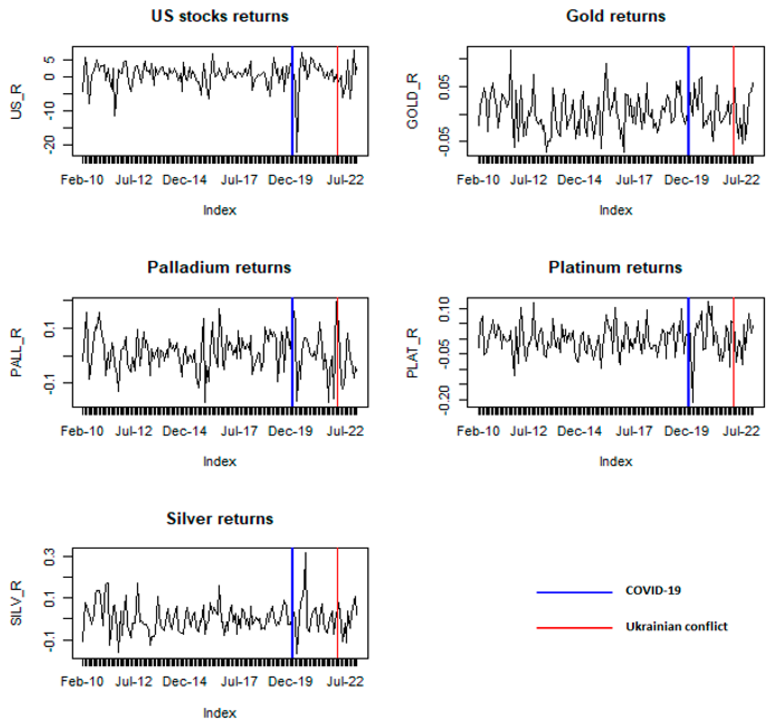
This is also evident in the respective plots for each series included in Figure 1, where the vertical blue line marks the outbreak of the COVID-19 pandemic, dividing the sample into the two phases. It can be observed that immediately after the beginning of the COVID-19 pandemic, there was a large decline in US stock returns, followed by a recovery, then a short period of gradual decline and a subsequent increase in prices towards the end of the series.
This increase coincides with the beginning of the Ukrainian conflict on the 24 February 2022, marked with the thick red vertical line in Figure 1. Collectively, these movements in US stocks increased the standard deviation of returns during the turbulent period. With the outbreak of the COVID-19 pandemic, declines were also observed for palladium, platinum, and silver; however, these series quickly returned to their pre-COVID-19 levels.
The large increase in the volatility of US stock returns should be expected to cause a bias in the correlation coefficient estimates between US stocks and the precious metal returns, leading to misleading inferences concerning their comovements. Table 2 summarizes these correlation coefficient estimates for the different periods. First, we provide results using the conditional (on heteroscedasticity) correlation coefficient for the stable and turbulent subperiods separately, and then for the full sample that covers both phases. With the exception of palladium returns, it can be observed that in all cases, there is a noticeable increase in the size of the correlation coefficient in the turbulent period, which is also evident (albeit to a smaller extent) in the full period sample estimates.
The unconditional correlation coefficient estimates between the US stocks and precious metal returns are presented in the rightmost column in Table 2. In all cases, the coefficient estimates are smaller, because the unconditional correlation coefficient corrects the heteroscedasticity bias associated with the conditional correlation coefficient. For palladium, platinum, and silver, these reductions are considerable with potential implications for the resource allocation decisions of the investors interested in these assets.
To investigate the synchronization of comovements between the different asset classes, we constructed separate correlation matrices using both the conditional and unconditional correlation coefficient estimates. These were subsequently used to derive correlation distance metrics that were used in an MSA, with the purpose of generating two-dimensional configurations that depict the similarities or dissimilarities between the financial returns. The correlation matrices are included in Appendix A.
Table 3 includes the results of the model fit criteria presented in Equation (5) for the MSA applications examined. The scores in column 2 correspond to two-dimensional configurations and are analogous in the case for the other columns (e.g., column 3 is for three-dimensional configurations). All scores included in column 2 are higher than 0.8 which, as explained in Section 3, indicates a good fit to the data. It is also worth mentioning that the configurations generated with the unconditional distance metric in Equation (4) provided the best fit to the data of all the two-dimensional configurations. Similarly, Camacho et al. (2006), Aguiar-Conraria et al. (2013) and Michis (2021) used two-dimensional configurations for the representations of economic time series.
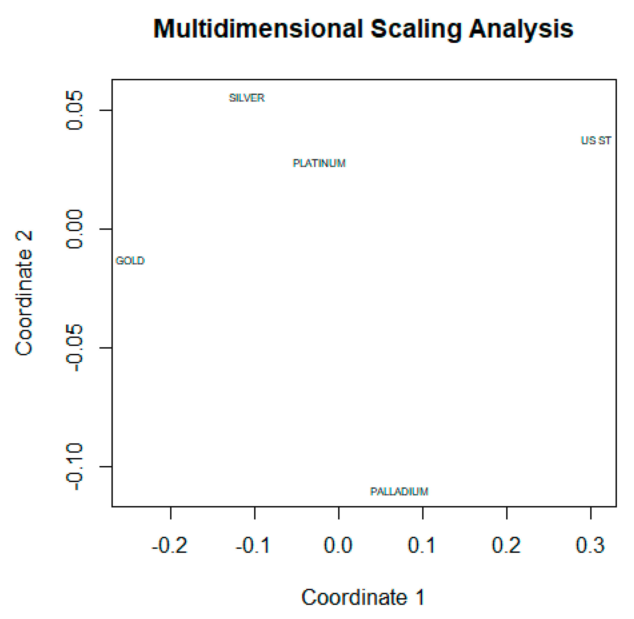
The two-dimensional configurations for the stable and turbulent periods, derived from the conditional correlation matrices in Appendix A, are included in Figure 2 and Figure 3, respectively. The results in Figure 2 suggest three distinct, and therefore, dissimilar, comovement asset returns: gold, palladium, and US stocks (US ST). Thus, during the stable period, gold and platinum could have potentially provided diversification benefits when included in portfolios that track the movements of the US stock market index. Silver and platinum are located closer to US stocks in the two-dimensional space, suggesting greater similarity with US stocks compared with the other precious metals.
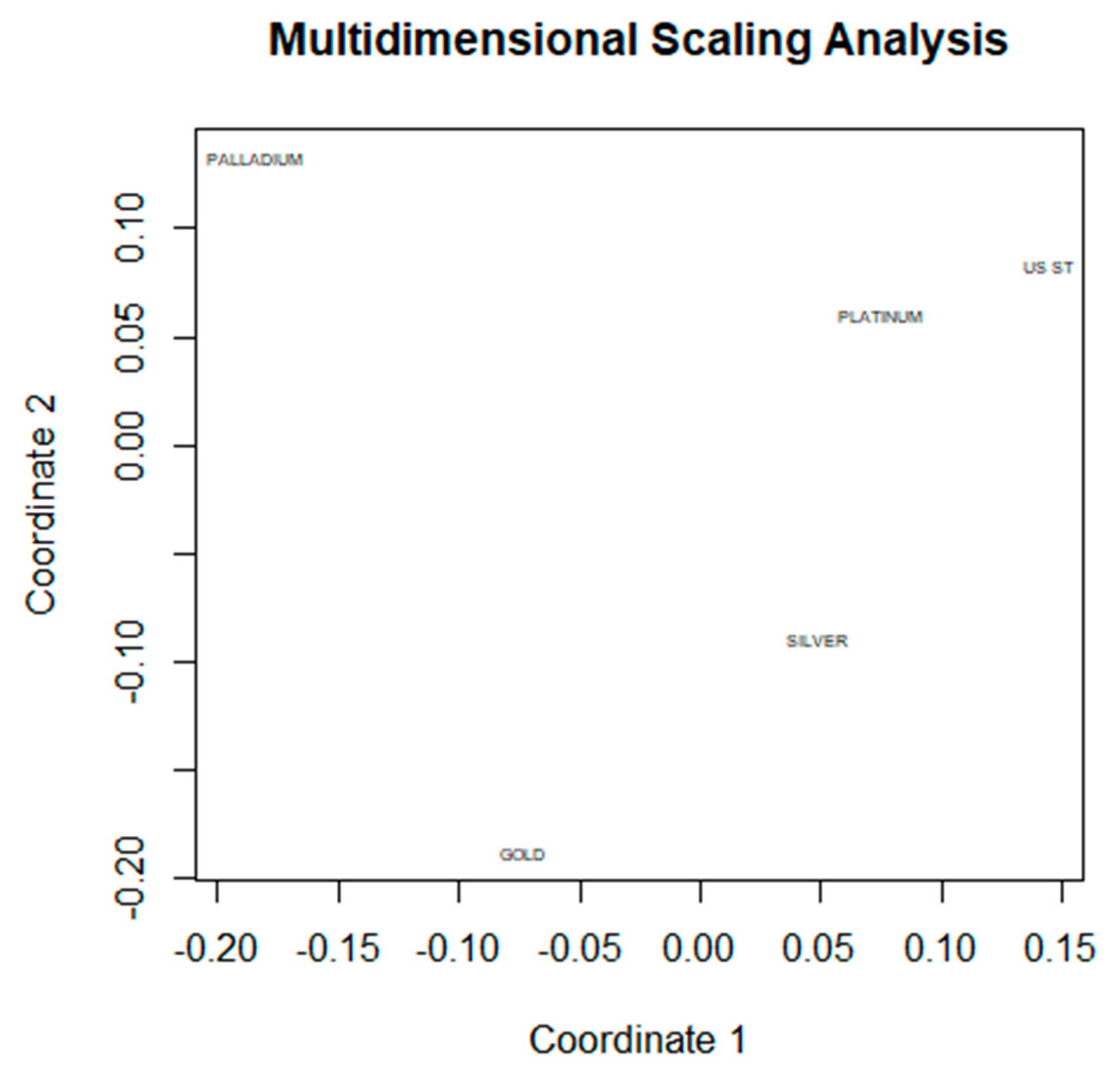
When considering the configurations in Figure 3 for the turbulent phase, two basic conclusions emerge. First, gold, palladium, and US stocks continue to be located further apart (albeit with different distances compared with Figure 2), suggesting that the financial return movements of gold and palladium continued to be dissimilar and less synchronized to US stocks, and are therefore useful for diversification purposes during the phase. Second, platinum is located closer to US stocks, while silver is still located halfway between US stocks and gold. These changes are also reflected in the respective conditional correlation matrices in Appendix A.
Figure 4 provides a two-dimensional configuration based on the unconditional correlation matrix across the two periods (full sample), using the distance metric in Equation (4) in the context of MSA. It can be observed that when correcting the heteroscedasticity bias in the estimated correlations, the two-dimensional configuration becomes more similar to the configuration in Figure 2 for the stable period.
Gold, palladium, and US stocks are located further apart, suggesting a dissimilarity in their financial returns. Therefore, these precious metals remain useful considerations for portfolios that track the US stock market index, because they can provide diversification benefits. Furthermore, compared with the configuration in Figure 2, silver and platinum are located closer to gold in Figure 4, which suggests financial return movements that are more synchronized with gold returns and less similar to US stock returns. This similarity is more pronounced in the case of silver.

4.2. Tests for Normality, Variance Stabilization and Sample Size Adjustment

In addition to the correlation estimates for the different periods, Table 2 also includes the results of t-tests for the null hypothesis of zero correlation (Chen and Popovich 2002) between the financial returns. According to the results, only the correlation estimates between US stocks and gold returns were not found to be significantly different from zero (except for the conditional correlation estimate in the turbulent period). However, when working with non-normal data, the t-test becomes problematic and Type I error rates tend to be inflated (Bishara and Hittner 2012).
Figure 5 includes density histograms for all the variables considered in this study. It can be observed that for some of the return series asymmetries exist that suggest departures from normality, such as the skewness of gold returns and the asymmetric tails of US stock returns. The normality assumption for the return series was also evaluated using the well-known Shapiro–Wilk and Kolmogorov–Smirnov normality tests that are frequently used in applied work (Romão et al. 2010). The p-values derived from these tests are included in Table 4. The normality assumption was accepted only for the gold and palladium time series when using the Shapiro–Wilk test (at either the 5% or 10% significance level), while it was rejected for all the time series when using the Kolmogorov–Smirnov test.
When normality does not hold alternative non-parametric methods of statistical inference need to be used (Lee and Rodgers 1998). For the purposes of this study we used a bias-corrected accelerated bootstrap resampling procedure with 999 replications, (Efron and Tibshirani 1994) to generate two-sided 95% confidence intervals for the correlation estimates in Table 2. The computations were performed with the confintr package for R, available from the CRAN archive and the generated confidence intervals are included in Table 5. The results indicate that for all reported periods, the correlation estimates in Table 2 fall within the corresponding bootstrap confidence intervals of Table 5.
Forbes and Rigobon (2002) showed that the heteroscedasticity bias in the conditional correlation formula is due to parameter  δ , which is the relative increase in the variance of  x , not the variance of the regression coefficient in the linear model (1). Since the conditional correlation coefficient is increasing in  δ , conditional correlation estimates will tend to increase in volatile periods, even if the underlying unconditional correlation coefficient remains the same.
To demonstrate this, we also applied a variance stabilization transform to the time series before proceeding with the correlation estimates, using the power transformation proposed by Yeo and Johnson (2000). This transformation can be seen as a generalization of the Box–Cox transformation (Greene 2018), which is frequently used in variance stabilization applications (Michis and Nason 2017). With strictly positive data, the two transforms become equal; however, the Yeo–Johnson transformation can also handle time series with negative observations. The transformation parameter in our application was estimated through the maximization of a log-likelihood criterion function (Raymaekers and Rousseeuw 2021) and the Yeo–Johnson transformation was implemented using the VGAM and car packages for R, available from the CRAN archive.
The correlation coefficient estimates for the different periods are summarized in Table 6. The differences in the conditional correlation estimates between the reported periods are similar to those included in Table 2. With the exception of palladium returns, in all cases, there is a noticeable increase in the size of the conditional correlation coefficient in the turbulent period, which is also evident in the full period estimates.
Despite the application of the variance stabilization procedure, the conditional correlation coefficient is still biased upwards due to the structural change in the variance of US stock returns in the turbulent period ( σ x x h > σ x x l ). In contrast, the unconditional correlation estimates are in all cases smaller, which underlines the importance of correcting the heteroskedasticity bias using Formula (2). This formula is specifically designed to adjust the conditional correlation estimate based on the value of parameter  δ .
As an additional robustness check for our results, we also estimated the “Phase I” stable period correlation coefficients using a reduced sample size that covers only the period January 2017–December 2019. The available observations for the period February 2010–December 2016 were excluded due to the existence of some other minor economic downturns and stock market volatility events within this time interval. Specifically, the European debt crisis concerns in 2011, the downgrade of US credit rating in August 2011, the Flash Crash of 2010 and the 2015–2016 stock market sell-off.
Even though these events did not escalate into full-blown economic crises, they can complicate inference from our correlation coefficient estimates, since “Phase I” (stable period) is considered as a benchmark for evaluating the correlation changes in “Phase II” (the turbulent period). The correlation coefficient estimates for this alternative stable period are included in Table 7. The full period estimates for both the conditional and unconditional correlation coefficients were also derived using a reduced sample size (January 2017–January 2023).
In this case too, the differences in the conditional correlation estimates between the reported periods are similar to those reported in Table 2. There is a noticeable increase in the size of the conditional correlation coefficients in the turbulent period, which is also evident in the full period sample estimates. This heteroscedasticity bias is corrected when the unconditional correlation coefficient is used, as demonstrated in the last column of Table 7. Furthermore, the unconditional correlation levels are similar to those reported in Table 2. However, it is important to emphasize that with the exception of platinum returns, all other conditional correlation coefficient estimates for the alternative stable period are not statistically significant at the 5% or 10% level and, therefore, these results should be used with caution.

4.3. Discussion

The theoretical foundation of our proposed method derives from the financial contagion literature and the large increases in cross-correlations observed between financial market indices when a financial crisis (shock) hits one of the interdependent countries. Forbes and Rigobon (2002) note that in such cases, large movements in one major stock market (e.g., the US stock market crash in 1987) tend to be associated with similarly large movements in other interconnected markets.
However, since correlation estimates are conditional on market volatility, they are biased upwards, providing the wrong impression of a large increase in cross-market linkages and, therefore, financial contagion. In contrast, the authors showed that adjusting this bias deflates the correlation estimates, suggesting only interdependence between the markets, which is a condition that exists across all phases of the economy.
Our study provides similar evidence for the cross market linkages that exist between US stocks and precious metal returns. These linkages derive from the investment characteristics of precious metals, which as explained in Section 2 are considered by investors as possessing hedging and safe haven properties in times of financial distress. For example, Mishkin (2016) notes the following factors as important determinants for the demand for gold: lower perceived riskiness relative to other assets, higher expected returns relative to other assets and higher liquidity relative to other assets.
The transmission mechanism in this case most commonly begins with a shock to the US stock market, which generates renewed interest for investments in precious metals (the “flight to quality” effect). When correlation estimates between US stocks and precious metal returns are performed during this period of increased market volatility, the results will be biased upwards, providing misleading inferences to investors seeking to adjust their investment portfolios. The large movements in US stocks are erroneously perceived as being associated with a significant increase in the linkages between US stocks and precious metal returns.
In contrast, the standard deviation changes in Table 1 (e.g., for US stocks and gold returns) between the stable and turbulent periods, do not provide any evidence for this assertion (increasing for US stock returns but not for gold returns). As demonstrated in Table 2, adjusting the heteroscedasticity bias using the unconditional correlation coefficient provides estimates that are closer to the levels estimated with the conditional correlation coefficient for the stable period. These estimates represent the interdependence that exists between US stock and precious metal returns in all phases of the financial system.
Most existing studies in the literature rely on dynamic conditional correlation GARCH models that suggest an increase in the correlation levels during times of financial distress. For example, Creti et al. (2013) found that the 2007–2008 financial crisis strengthened the links of commodities (including metals) with stock markets, and Sadorsky (2014) reported an increase in the correlation levels between emerging market stocks, copper, oil and wheat since 2008.
Furthermore, the empirical results of Mensi et al. (2017) provide strong evidence of volatility spillovers between stocks and precious metals since the global financial crisis of 2007–2008 and the European sovereign debt crisis of 2010–2012. Interestingly, the authors found precious metals to be the net recipients and the stocks the source of the spillovers. Similarly, Junttila et al. (2018) found the correlation levels between equity returns and gold to have increased since the 2008 financial crisis.
Our results provide a different perspective on the correlation levels observed between stock market and precious metal returns across different phases of the economy, concentrating on the turbulent period that began with the outbreak of the COVID-19 pandemic. While we agree with Mensi et al. (2017) that the transmission mechanism between stocks and precious metals is indicative of contagion effects, as suggested in the financial contagion literature, our results are more compatible with the analysis of Forbes and Rigobon (2002) who provided a critical evaluation of the financial contagion literature.
According to the authors, since correlation coefficient estimates are conditional on market volatility, they will tend to increase significantly following a shock, giving the impression of an increase in cross-market linkages and, therefore, the existence of strong financial contagion effects from one stock market to other markets. When this heteroscedasticity bias is corrected, as in the case of the unconditional correlation coefficient, a different level of market linkages can exist, which is more compatible with the pre-existing conditions and the underlying long-term interdependence between the markets, not contagion.
The results reported in Section 4 for the stock market–precious metals linkages are more compatible with the second case. After correcting the heteroscedasticity bias introduced by the COVID-19 pandemic and the subsequent Ukrainian conflict, the correlation levels of gold, silver, platinum, and palladium returns with US stock returns were not found to have changed substantially during Phase II. They are more compatible with the stable period (Phase I) considered in our analysis, suggesting a continuation of the interdependence levels that existed prior to the pandemic.
Our methodology and results will be of interest to investors considering the synthesis of their portfolios or the adoption of hedging strategies during turbulent periods. For example, resisting the temptation to make large changes in the synthesis of their portfolios when the underlying cross-market correlations between asset returns have not changed significantly, or to construct effective hedge ratios by hedging a long position in US stocks using a short position in a carefully selected precious metal. In this respect, the results in Section 4 suggest that gold and palladium can be useful considerations for hedging long positions in US stocks.
We also note two results from the aforementioned literature that are consistent with our analysis in Section 4. First, Mensi et al. (2017) found stock markets to be the source and precious metals the net recipients of volatility slipovers during financial crises. This is consistent with our definition of US stock returns, as the benchmark source financial variable in all applications of the unconditional correlation formula in Section 4.
Second, the results by Uddin et al. (2020) suggest a similarity in the behaviour of silver and platinum returns towards US stocks during market downturns and a rather different behaviour in the case of gold, whose relationship with US stocks was found to be weaker. These associations are compatible with our graphical analysis in Section 4 where silver and platinum are depicted closer together and with US stocks in the two-dimensional configurations, while gold is always located further away.

5. Conclusions

In this study, we examined the evolution of correlation estimates between US stocks and four precious metal returns (gold, silver, palladium, and platinum) over two phases: before and after the outbreak of the COVID-19 pandemic. The later phase was also extended to include the beginning of the Ukrainian conflict, which coincided with the first transition of COVID-19 to endemic status in the USA. Due to the increase in the volatility of the US stock market index observed after the outbreak of the COVID-19 pandemic, the heteroskedasticity-adjusted unconditional correlation coefficient proposed by Forbes and Rigobon (2002) was used to examine the evolution of correlation changes across the two phases. In addition, a relevant correlation distance metric was proposed in the context of MSA to examine the associations (similarities or dissimilarities) between US stock and precious metal returns over the examined period.
Our findings suggest the existence of an upward heteroscedasticity bias in most correlation estimates due to the increase in market volatility in the post-COVID-19 period. When corrected, the correlation levels of gold, silver, platinum, and palladium returns with US stock returns were not found to have changed substantially since the COVID-19 outbreak.
Furthermore, an MSA of the comovements between the financial returns of US stocks and the four precious metals, using the heteroscedasticity-adjusted distance metric, provided two main insights for investors. First, gold and palladium can provide useful additions in portfolios that track the US stock market index, because they exhibit less similarity to the movements of US stocks. Second, silver and platinum exhibit movements that are more synchronized with gold returns but are less dissimilar to US stock returns, compared with gold and palladium returns.

Funding

This research received no external funding.

Institutional Review Board Statement

Not applicable.

Informed Consent Statement

Not applicable.

Data Availability Statement

Data are available upon request.

Conflicts of Interest

The author declares no conflict of interest.

Appendix A

Table A1. Conditional correlation matrix: stable period.
US StocksGoldPalladiumPlatinumSilver
US stocks1–0.1150.4730.3640.182
Gold–0.11510.3720.6400.785
Palladium0.4730.37210.6220.498
Platinum0.3640.6400.62210.668
Silver0.1820.7850.4980.6681
Table A2. Conditional correlation matrix: turbulent period.
US StocksGoldPalladiumPlatinumSilver
US stocks10.3000.3050.7110.589
Gold0.30010.3160.3980.710
Palladium0.3050.31610.4250.342
Platinum0.7110.3980.42510.713
Silver0.5890.7100.3420.7131
Table A3. Unconditional correlation matrix: full period.
US StocksGoldPalladiumPlatinumSilver
US stocks10.0150.2480.3300.210
Gold0.01510.3430.5580.758
Palladium0.2480.34310.5340.432
Platinum0.3300.5580.53410.685
Silver0.2100.7580.4320.6851

References

  1. Aguiar-Conraria, Luís, and Maria Joana Soares. 2011. Business cycle synchronization and the euro: A wavelet analysis. Journal of Macroeconomics 33: 477–89. [Google Scholar] [CrossRef]
  2. Aguiar-Conraria, Luís, Manuel M.F. Martins, and Maria Joana Soares. 2013. Convergence of the economic sentiment cycles in the Eurozone: A time-frequency analysis. Journal of Common Market Studies 51: 377–98. [Google Scholar] [CrossRef]
  3. Akhtaruzzaman, Md, Sabri Boubaker, Brian M. Lucey, and Ahmet Sensoy. 2021. Is gold a hedgeor safe-haven asset in the COVID-19 crisis? Economic Modelling 102: 105588. [Google Scholar] [CrossRef]
  4. Bahloul, Slah, and Imen Khemakhem. 2021. Dynamic return and volatility connectedness between commodities and Islamic stock market indices. Resources Policy 71: 101993. [Google Scholar] [CrossRef]
  5. Baur, Dirk G., and Brian M. Lucey. 2010. Is gold a hedge or a safe-haven? An analysis of stocks, bonds and gold. Financial Review 45: 217–29. [Google Scholar] [CrossRef]
  6. Bishara, Anthony J., and James B. Hittner. 2012. Testing the Significance of a correlation with nonnormal data: Comparison of Pearson, Spearman, transformation, and resampling approaches. Psychological Methods 17: 399–417. [Google Scholar] [CrossRef]
  7. Bouri, Elie, Oguzhan Cepni, Davi Gabauer, and Rangan Gupta. 2021. Return connectedness across asset classes around the COVID-19 outbreak. International Review of Financial Analysis 73: 101646. [Google Scholar] [CrossRef]
  8. Camacho, Maximo, Gabriel Perez-Quiros, and Lorena Saiz. 2006. Are European business cycles close enough to be just one? Journal of Economic Dynamics and Control 30: 1678–706. [Google Scholar] [CrossRef]
  9. Chemkha, Rahma, Ahmet BenSaïda, Ahmet Ghorbel, and Tahar Tayachi. 2021. Hedge and safe haven properties during COVID-19: Evidence from Bitcoin and gold. The Quarterly Review of Economics and Finance 82: 71–85. [Google Scholar] [CrossRef]
  10. Chen, Peter Y., and Paula M. Popovich. 2002. Correlation: Parametric and Nonparametric Measures. Thousand Oaks: Sage publications. [Google Scholar]
  11. Chiang, Thomas C., Lin Tan, and Huimin Li. 2007. Empirical analysis of dynamic correlations of stock returns: Evidence from Chinese A-share and B-share markets. Quantitative Finance 7: 651–67. [Google Scholar] [CrossRef]
  12. Conover, Mitchell C., Gerald R. Jensen, Robert R. Johnson, and Jeffrey M. Mercer. 2009. Can precious metals make your portfolio shine? Journal of Investing 18: 75–86. [Google Scholar] [CrossRef]
  13. Corbet, Shaen, Charles Larkin, and Brian Lucey. 2020. The contagion effects of the COVID-19 pandemic: Evidence from gold and cryptocurrencies. Finance Research Letters 35: 101554. [Google Scholar] [CrossRef]
  14. Cox, Mike A. A. 2013. Analysis of stock market indices through multidimensional scaling. Journal of Statistical Computation and Simulation 83: 2015–29. [Google Scholar] [CrossRef]
  15. Cox, Trevor F. 2005. An Introduction to Multivariate Statistical Analysis. London: Hodder Arnold. [Google Scholar]
  16. Creamer, Germán G., and Chihoon Lee. 2019. A multivariate distance nonlinear causality test based on partial distance correlation: A machine learning application to energy futures. Quantitative Finance 19: 1531–42. [Google Scholar] [CrossRef]
  17. Creti, Anna, Marc Joëts, and Valérie Mignon. 2013. On the links between stock and commodity markets’ volatility. Energy Economics 37: 16–28. [Google Scholar] [CrossRef]
  18. Efron, Bradley, and Robert J. Tibshirani. 1994. An Introduction to the Bootstrap. Boca Raton: Chapman & Hall/CRC. [Google Scholar]
  19. Engle, Robert, and Riccardo Colacito. 2006. Testing and Valuing Dynamic Correlations for Asset Allocation. Journal of Business & Economic Statistics 24: 238–53. [Google Scholar]
  20. Everitt, Brian, and Torsten Hothorn. 2011. An Introduction to Applied Multivariate Analysis with R. New York: Springer. [Google Scholar]
  21. Forbes, Kristin J., and Roberto Rigobon. 2002. No contagion, only interdependence: Measuring stock market comovements. Journal of Finance 57: 2223–61. [Google Scholar]
  22. Geertsema, Paul, and Helen Lu. 2020. The correlation structure of anomaly strategies. Journal of Banking and Finance 119: 105934. [Google Scholar] [CrossRef]
  23. Gharib, Cheima, Salma Mefteh-Wali, and Sami Ben Jabeur. 2021. The bubble contagion effect of COVID-19 outbreak: Evidence from crude oil and gold markets. Finance Research Letters 38: 101703. [Google Scholar] [CrossRef]
  24. Greene, William H. 2018. Econometric Analysis, 8th ed. New York: Pearson Education. [Google Scholar]
  25. Ji, Qiang, Dayong Zhang, and Yuqian Zhao. 2020. Searching for safe-haven assets during the COVID-19 pandemic. International Review of Financial Analysis 71: 101526. [Google Scholar] [CrossRef]
  26. Joy, Mark. 2011. Gold and the US dollar: Hedge or heaven? Finance Research Letters 8: 120–31. [Google Scholar] [CrossRef]
  27. Jung, Sean S., and Woojin Chang. 2016. Clustering stocks using partial correlation coefficients. Physica A 462: 410–20. [Google Scholar] [CrossRef]
  28. Junttila, Juha, Juho Pesonen, and Juhani Raatikainen. 2018. Commodity market based hedging against stock market risk in times of financial crisis: The case of crude oil and gold. Journal of International Financial Markets, Institutions and Money 56: 255–80. [Google Scholar] [CrossRef]
  29. Kenett, Dror Y., Xuqinq Huang, Irena Vodenska, Shlomo Havlin, and Eugene H. Stanley. 2015. Partial correlation analysis: Applications for financial markets. Quantitative Finance 15: 569–78. [Google Scholar] [CrossRef]
  30. Krishnan, C. N. V., Ralitsa Petkova, and Peter Ritchken. 2009. Correlation risk. Journal of Empirical Finance 16: 353–67. [Google Scholar] [CrossRef]
  31. Kumar, Anoop S., and Steven Raj Padakandla. 2022. Testing the safe-heaven properties of gold and bitcoin in the backdrop of COVID-19: A wavelet quantile correlation approach. Finance Research Letters 47: 102707. [Google Scholar] [CrossRef]
  32. Lahiani, Amine, Salma Mefteh-Wali, and Dinara G. Vasbieva. 2021. The safe-heaven property of precious metal commodities in the COVID-19 era. Resources Policy 74: 102340. [Google Scholar] [CrossRef]
  33. Lee, Won-Chan, and Joseph Lee Rodgers. 1998. Bootstrapping correlation coefficients using univariate and bivariate sampling. Psychological Methods 3: 91–103. [Google Scholar] [CrossRef]
  34. Loretan, Miko, and William B. English. 2000. Evaluating “correlation breakdowns” during periods of market volatility. In Bank for International Settlements: International Financial Markets and the Implications for Monetary and Financial Stability. Basel: Bank of International Settlements. [Google Scholar]
  35. Lucey, Brian M., and Sile Li. 2015. What precious metals act as safe havens, and when? Some US evidence. Applied Economics Letters 22: 35–45. [Google Scholar] [CrossRef]
  36. Machado, Tenreiro J., Fernando B. Duarte, and Gonçalo M. Duarte. 2011. Analysis of financial data series using fractional Fourier transform and multidimensional scaling. Nonlinear Dynamics 65: 235–45. [Google Scholar] [CrossRef]
  37. Mensi, Walid, Khamis Hamed Al-Yahyaee, and Khamis Hamed Kang. 2017. Time-varying volatility spillovers between stock and precious metal markets with portfolio implications. Resources Policy 53: 88–102. [Google Scholar] [CrossRef]
  38. Mensi, Walid, Makram Beljid, Adel Boubaker, and Shunsuke Managi. 2013. Correlations and volatility spillovers across commodity and stock markets: Linking energies, food, and gold. Economic Modelling 32: 15–22. [Google Scholar] [CrossRef]
  39. Michis, Antonis A. 2014. Investing in Gold: Individual Asset Risk in the Long-Run. Finance Research Letters 11: 369–74. [Google Scholar] [CrossRef]
  40. Michis, Antonis A. 2019. The systematic risk of gold at different time-scales. Economics Bulletin 39: 1215–27. [Google Scholar]
  41. Michis, Antonis A. 2021. Wavelet multidimensional scaling analysis of European economic sentiment indicators. Journal of Classification 38: 443–80. [Google Scholar] [CrossRef]
  42. Michis, Antonis A. 2022. Multiscale partial correlation clustering of stock market returns. Journal of Risk and Financial Management 15: 24. [Google Scholar] [CrossRef]
  43. Michis, Antonis A., and Guy P. Nason. 2017. Case study: Shipping trend estimation and prediction via multiscale variance stabilization. Journal of Applied Statistics 44: 2672–84. [Google Scholar] [CrossRef]
  44. Mishkin, Frederic S. 2016. The Economics of Money Banking and Financial Markets. Essex: Pearson education. [Google Scholar]
  45. Peng, Xiaofan. 2020. Do precious metals act as hedges or safe havens for China’s financial markets? Finance Research Letters 37: 101353. [Google Scholar] [CrossRef]
  46. Raymaekers, Jacob, and Peter J. Rousseeuw. 2021. Transforming variables to central normality. Machine Learning 1–23. [Google Scholar] [CrossRef]
  47. Reboredo, Juan C. 2013. Is gold a safe haven or a hedge for the US dollar? Implications for risk management. Journal of Banking & Finance 37: 2665–76. [Google Scholar]
  48. Romão, Xavier, Raimundo Delgado, and Aníbal Costa. 2010. An empirical power comparison of univariate goodness-of-fit tests for normality. Journal of Statistical Computation and Simulation 80: 545–91. [Google Scholar] [CrossRef]
  49. Ronn, Ehud. 1998. The Impact of Large Changes in Asset prices on Intra-Market Correlations in the Stock and Bond Markets. Manuscript. Austin, TX, USA: Department of Finance, University of Texas. [Google Scholar]
  50. Sadorsky, Perry. 2014. Modeling volatility and correlations between emerging market stock prices and the prices of copper, oil and wheat. Energy Economics 43: 72–81. [Google Scholar] [CrossRef]
  51. Salisu, Afees A., Ibrahim D. Raheem, and Xuan Vinh Vo. 2021. Assesing the safe heaven property of the gold market during COVID-19 pandemic. International Review of Financial Analysis 74: 101666. [Google Scholar] [CrossRef] [PubMed]
  52. Skiadopoulos, George. 2012. Investing in commodities: Popular beliefs and misconceptions. Journal of Asset Management 13: 77–83. [Google Scholar] [CrossRef]
  53. Uddin, Gazi Salah, Jose Arreola Hernandez, Syed Jawad Hussain Shahzad, and Sang Hoon Kang. 2020. Characteristics of spillovers between the US stock market and precious metals and oil. Resources Policy 66: 101601. [Google Scholar] [CrossRef]
  54. Wątorek, Marcin, Stanisław Drożdż, Paweł Oświȩcimka, and Marek Stanuszek. 2019. Multifractal cross-correlations between the world oil and other financial markets in 2012–17. Energy Economics 81: 874–85. [Google Scholar] [CrossRef]
  55. Yeo, In-Kwon, and Richard A. Johnson. 2000. A new family of power transformations to improve normality or symmetry. Biometrika 87: 954–59. [Google Scholar] [CrossRef]
  56. Yousaf, Imran, Elie Bouri, Shoaib Ali, and Nehme Azoury. 2021. Gold against Asian stock markets during the COVID-19 outbreak. Journal of Risk and Financial Management 14: 186. [Google Scholar] [CrossRef]
Figure 1. Financial returns: US stocks and precious metals.
Jrfm 16 00280 g001
Figure 2. MSA using the conditional correlation matrix: stable period.
Jrfm 16 00280 g002
Figure 3. MSA using the conditional correlation matrix: turbulent period.
Jrfm 16 00280 g003
Figure 4. MSA using the unconditional correlation matrix: full period.
Jrfm 16 00280 g004
Figure 5. Density histograms of financial returns.
Jrfm 16 00280 g005
Table 1. Summary statistics of financial returns.
US StocksGoldPalladiumPlatinumSilver
Stable period
Mean0.5790.0030.014–0.0030.002
Median0.9930.0010.019–0.005–0.011
Stand. Dev.2.8880.0340.0620.0450.063
Min–11.468–0.068–0.170–0.122–0.162
Max6.7480.1160.1680.1200.172
Turbulent period
Mean0.4930.0070.0010.0060.012
Median1.1780.000–0.0010.0180.008
Stand. Dev.4.9130.0340.0910.0660.084
Min–21.940–0.053–0.170–0.210–0.168
Max7.6630.0680.1960.1230.318
Table 2. Correlations of US stocks with precious metals.
CorrelationConditionalUnconditional
PeriodStableTurbulentFullFull
US stocks—Gold–0.1150.300 **0.0250.015
US stocks—Palladium0.473 *0.305 **0.399 *0.248 *
US stocks—Platinum0.364 *0.711 *0.511 *0.330 *
US stocks—Silver0.182 *0.589 *0.344 *0.210 *
Note: statistically significant values at: * 5%, ** 10% (t-test:  H 0 : ρ = 0  vs.  H 1 : ρ 0 ).
Table 3. Multidimensional scaling analysis of goodness-of-fit measures.
12345
Absolute eigenvalues
Stable—conditional correlation0.7880.8680.9160.9161.000
Turbulent—conditional correlation0.4650.9240.9790.9791.000
Full—conditional correlation0.6910.9350.9881.0001.000
Squared eigenvalues
Stable—conditional correlation0.9750.9850.9890.9891.000
Turbulent—conditional correlation0.5020.9920.9980.9991.000
Full—conditional correlation0.8840.9950.9991.0001.000
Table 4. p-values for normality tests on the asset returns.
Shapiro—WilkKolmogorov—Smirnov
US stocks<0.001<0.001
Gold0.381<0.001
Palladium0.630<0.001
Platinum0.061<0.001
Silver0.001<0.001
Table 5. Confidence intervals for correlations of US stocks with precious metals.
CorrelationConditionalUnconditional
PeriodStableTurbulentFullFull
US stocks—Gold–0.420–0.1030.004–0.526–0.268–0.188–0.139–0.107
US stocks—Palladium0.288–0.5980.037–0.6330.232–0.5370.148–0.344
US stocks—Platinum0.158–0.4870.436–0.8980.355–0.6910.224–0.505
US stocks—Silver–0.001–0.3500.369–0.7640.174–0.4810.107–0.320
Note: 95% bootstrap confidence intervals for the unconditional correlation coefficient.
Table 6. Correlations of US stocks with precious metals: Yeo–Johnson transformation.
CorrelationConditionalUnconditional
PeriodStableTurbulentFullFull
US stocks—Gold–0.0480.329 *0.0710.047
US stocks—Palladium0.498*0.2390.390 *0.270 *
US stocks—Platinum0.406*0.698 *0.523 *0.376 *
US stocks—Silver0.204*0.671 *0.374 *0.258 *
Note: statistically significant values at: * 5%, (t-test:  H 0 : ρ = 0  vs.  H 1 : ρ 0 ).
Table 7. Correlations of US stocks with precious metals: alternative stable period.
CorrelationConditionalUnconditional
PeriodStableTurbulentFullFull
US stocks—Gold–0.0670.300 **0.198 **0.098
US stocks—Palladium0.2430.305 **0.289 *0.146 **
US stocks—Platinum0.335 *0.711 *0.619 *0.360 *
US stocks—Silver–0.0210.589 *0.474 *0.255 *
Note: statistically significant values at: * 5%, ** 10% (t-test:  H 0 : ρ = 0  vs.  H 1 : ρ 0 ).
Disclaimer/Publisher’s Note: The statements, opinions and data contained in all publications are solely those of the individual author(s) and contributor(s) and not of MDPI and/or the editor(s). MDPI and/or the editor(s) disclaim responsibility for any injury to people or property resulting from any ideas, methods, instructions or products referred to in the content.

