Article

Assessing the Use of Gold as a Zero-Beta Asset in Empirical Asset Pricing: Application to the US Equity Market

1
Coventry Business School, Coventry University, Gosford Street, Coventry CV1 5DL, UK
2
Faculty of Business and Justice, The university of Central Lancashire, Preston PR1 2HE, UK
3
Department of Management, Faculty of Commerce, Mansoura University, Mansoura 35516, Egypt
4
Alliance Manchester Business School, The University of Manchester, Manchester M13 9PL, UK
5
Brunel Business School, Brunel University London, London UB8 3PH, UK
6
Department of Accounting, Faculty of Commerce, Mansoura University, Mansoura 35516, Egypt
7
Newcastle University Business School, Newcastle University, Newcastle upon Tyne, NE4 5TG, UK
8
Department of Business Administration, Faculty of Commerce, Zagazig University, Zagazig 44519, Egypt
*
Author to whom correspondence should be addressed.
J. Risk Financial Manag. 2023, 16(3), 204; https://doi.org/10.3390/jrfm16030204
Submission received: 19 December 2022 / Revised: 24 February 2023 / Accepted: 1 March 2023 / Published: 15 March 2023
(This article belongs to the Special Issue Financial Markets, Financial Volatility and Beyond (Volume II))

Abstract

:
This paper examines the use of the return on gold instead of treasury bills in empirical asset pricing models for the US equity market. It builds upon previous research on the safe-haven, hedging, and zero-beta characteristics of gold in developed markets and the close relationship between interest rates, stock, and gold returns. In particular, we extend this research by showing that using gold as a zero-beta asset helps to improve the time-series performance of asset pricing models when pricing US equities and industries between 1981 and 2015. The performance of gold zero-beta models is also compared with traditional empirical factor models using the 1-month Treasury bill rate as the risk-free rate. Our results indicate that using gold as a zero-beta asset leads to higher R-squared values, lower Sharpe ratios of alphas, and fewer significant pricing errors in the time-series analysis. Similarly, the pricing of small stock and industry portfolios is improved. In cross-section, we also find improved results, with fewer cross-sectional pricing errors and more economically meaningful pricing of risk factors. We also find that a zero-beta gold factor constructed to be orthogonal to the Carhart four factors is significant in cross-section and helps to improve factor model performance on momentum portfolios. Furthermore, the Fama–French three- and five-factor asset pricing models and the Carhart model are all improved by these means, particularly on test assets which have been poorly priced by the traditional versions. Our results have salient implications for policymakers, governments, central bank rate-setting decisions, and investors.
JEL Classification:
C1; C2; C5; F3; G1

1. Introduction

The trade-off between risk and return is a fundamental concept in finance. The return on a risk-free asset is a crucial variable in financial equilibrium models, yet its selection and value have been a source of controversy. In the US equity market, Mehra and Prescott (1985) and Weil (1989) link the problem of a higher equity premium than predicted by theory to the puzzle of why the risk-free rate should be so low. Traditionally, the return on a treasury bill has been used as a proxy for the risk-free rate, but there has been ongoing debate regarding the appropriate tenor of the T-bill. As a result, researchers have utilized treasury securities with various maturities in order to enhance asset pricing models. For instance, Mehra and Prescott (1985) utilise a one-year rate, and Albuquerque et al. (2016) examine the applicability of 1-, 5-, and 20-year rates. Barberis et al. (2015) develop the assumption that a risk-free rate is constant over long periods, whereas Fama and French (1993) use a 1-month T-bill rate, which changes each month. He et al. (2022) examine gold, T-bills, Interbank Offered Rates (IBOR), and Overnight Index Swaps (OIS) to identify proxies for risk-free assets.
In this paper, we assume that the risk-free rate is constantly changing but question the nature of the asset used to derive this short-term rate. The return on Treasury bills is traditionally used as a risk-free rate in asset pricing models (Carhart 1997; Fama and French 1993, 2015, 2018, 2020). Treasury bills are presumed to constitute risk-free investments, since their issuing governments are viewed as ‘default-free’ entities that offer guaranteed investments. If governments default or the possibility of default arises, then their obligations do not remain guaranteed. Even for the United States, Nippani and Smith (2010) reveal that Treasury securities are not default-free, as they witnessed observed nonzero Credit Default Swap premia during the financial crisis. The same is doubly true of Treasury securities of less creditworthy states such as Mexico, Greece, Spain, and Italy. In the foundational market model of the Capital Asset Pricing Model (CAPM), the risk-free rate provides the foundation for estimating the cost of equity and the expected returns of risky assets or securities. If Treasury bills do not remain risk-free investments, then the application of the return on Treasury bills may not be the appropriate proxy for the risk-free rate. Given this, it is important to consider alternative assets to determine if they may be more appropriate proxies for the risk-free rate.
Using a correct proxy for the risk-free rate has remained an ongoing topic of debate among academicians and practitioners (He et al. 2022). In contrast to the return on debt issued by governments, gold has a long history of serving as a financial security and has been used as a form of currency in various countries. Gold has received significant attention in financial markets due to its remarkable performance during the global financial crisis of 2008, and researchers have labeled it a safe-haven asset since it acts as a stabilizing force for financial systems in developed markets (Baur and Lucey 2010; Baur and McDermott 2010; Long et al. 2021). The safe-haven, currency hedging, and diversification benefits of gold during the global financial crisis in 2008 have been reassessed and reaffirmed in other studies (e.g., Hoang et al. 2015; O’Connor et al. 2015). The prior literature also shows a close relationship between the gold return and the return on Treasury bills. Barro and Misra (2016) examine the returns on gold and US Treasury bills from 1836 to 2011 and reveal that the real price change in gold is close to the real return on Treasury bills. Additionally, it has been observed that gold prices react swiftly to changes in federal fund rates (Kontonikas et al. 2013).
Although gold is widely recognized as a safe-haven and hedging instrument, as supported by existing research (Bekiros et al. 2017; Faria and McAdam 2012; Gil-Alana et al. 2015; He et al. 2018; Nguyen et al. 2019; Wu and Chiu 2017; Cui et al. 2023), there has been a paucity of literature examining the use of gold as a zero-beta asset in asset pricing models. Previous studies by He et al. (2018, 2022) have explored gold, T-bills, Interbank Offered Rates (IBOR), and Overnight Index Swaps (OIS) to identify suitable proxies for risk-free assets. They have found that gold can serve as a proxy for risk-free assets in the United Kingdom and China, while for T-bills in Japan and IBOR in China. However, these studies fail to provide evidence for an appropriate proxy for the US market when applying a single-factor CAPM on a sample of S&P 500 stocks.
Therefore, this paper extends the existing empirical research by thoroughly investigating the applicability of gold as a zero-beta asset in traditional asset pricing models, utilizing a wide range of test assets in the US equity market. In the spirit of Black et al. (1972, hereafter BJS) and He et al. (2018), we use the returns on gold as the return on a zero-beta asset. Several studies have found gold to have a zero beta with respect to the market, as evidenced by Jaffe (1989), Chua et al. (1990), McCown and Zimmerman (2006), Baur and McDermott (2010), Blose (2010), Reboredo (2013), He et al. (2018).
Research by Wang et al. (2011) and Ntim et al. (2015) indicates weak-form efficiency in the US gold market, which is a desirable feature for assets to satisfy Arrow–Debreu conditions. This finding suggests that gold returns may be a better candidate to satisfy these conditions compared with the returns on Treasury bills, as noted by Constantinides and Duffie (1996). Before using gold in asset pricing models in the US equity market, we examine the criteria of the BJS’s zero-beta rate, specifically that gold shows zero beta, minimum variance, and efficiency. To this end, we perform variance-ratio tests to assess the efficiency of the gold market. Furthermore, we plot the minimum variance Frontier by using gold returns and different sets of test portfolios to test the criteria of the zero-beta rate.
Our study contributes to the existing literature in several significant ways. Firstly, we employ gold as a zero-beta asset in traditional asset pricing models on a wide range of test assets in the US equity market. We demonstrate that using gold in this way is preferable to the traditional use of the yield on a 1-month T-bill as a risk-free rate, which has significant theoretical limitations in terms of its suitability as a risk-free return. Secondly, we show that the return on gold lacks the shortcomings associated with T-bills and is therefore preferable on theoretical grounds. Furthermore, we find that asset pricing models which use gold as a zero-beta asset have better time-series and cross-sectional performance than traditional models using the T-bill risk-free rate. Thirdly, we investigate the extended Carhart (1997) and Fama and French (1993, 2015, 2017) models, ranging from three factors to six factors. To the best of our knowledge, no other paper has compared these six extended factor models together in a single study. We also conduct our analyses using both time-series and cross-sectional data. It is worth noting that our study is limited to using gold returns as a proxy for the zero-beta rate, rather than considering a portfolio of risky securities as proposed by Black et al. (1972) in their original zero-beta model. Our study assumes that using a zero-beta rate based on gold has advantages over a portfolio of risky assets due to gold’s traditional and historical safe-haven abilities. A portfolio of risky assets still faces a risk of losing its value in different time periods, whereas gold has maintained its reputation of retaining its value over centuries.
In the field of asset pricing, gold has been traditionally used in the Merton (1973) ICAPM framework to examine gold factor exposures in industry equity portfolio returns (Chan and Faff 2002; Davidson et al. 2003). However, we advance upon these by examining the employment of the gold return as a replacement for the risk-free rate, hitherto unexplored in the asset pricing literature. Furthermore, we provide a comprehensive comparison of the traditional Fama and French (1993, 2015, 2017) and Carhart (1997) models with those that employ gold as a zero-beta asset on an extensive range of test assets. For robustness and ease of comparison with Fama and French (2015), we assess the performance of these asset pricing models with and without small stocks and demonstrate improved pricing of small stocks. Ang et al. (2006) use a volatility factor to improve the performance of the Fama and French (1993) three-factor model on portfolios sorted by cash-flow volatility, and in a similar vein, we examine gold as a zero-beta asset to price portfolios sorted by variance. BJS relax the CAPM assumption that investors can borrow and lend freely and to an unlimited extent at the risk-free rate, as well as examine the CAPM with limited borrowing, permitting investors to lend but not borrow at the zero-beta rate. Similarly, we restrict investors from investing but not borrowing at the gold return rate.
Our results show that, in time series, models that employ gold as a zero-beta asset exhibit higher R-squared values, lower Sharpe ratios of alphas, and fewer significant pricing errors. We find that such models are better able to price portfolios of small stocks, where traditional models struggle. In cross-section, we find fewer cross-sectional pricing errors and economically plausible values of the market risk premium appearing for test assets where traditional models generate implausible negative prices of market risk. We show that the CAPM, the Fama and French (1993) three-factor model, the Carhart (1997) four-factor model, and the Fama and French (2015) five-factor model all exhibit improved asset pricing performance when using gold as a zero-beta asset. Furthermore, we find that there is information in the return on gold beyond that captured by the Carhart (1997) factors, as a gold return factor constructed to be orthogonal to these remains significant in cross-section when added to the Carhart (1997) model. This suggests that the use of gold as a zero-beta asset in asset pricing models captures additional variance not encompassed by the traditional factors. Overall, our study highlights the advantages of using gold as a zero-beta asset in equity asset pricing models and provides evidence for its superior performance over the traditional use of the yield on a 1-month T-bill as a risk-free rate.
The structure of this paper is as follows: Section 1 introduces the problems associated with the risk-free rate in empirical asset pricing and highlights the efficiency, hedging, and zero-beta characteristics of gold. Section 2 presents the theoretical framework of the zero-beta CAPM, explains the development of the extended versions of the traditional CAPM model, and discusses the relationships between interest rates, Treasury bills, gold, and stock prices. Section 3 describes the data used, and Section 4 briefly covers the methodology of the asset pricing tests. Section 5 presents the empirical findings, and Section 6 concludes.

2. Literature Review

2.1. The Development of the Zero-Beta Model

The CAPM was developed by Sharpe (1964), Lintner (1965), and Mossin (1966) as an advancement of Markowitz’s (1959) mean-variance theory. A principal assumption of the CAPM is that investors may lend or borrow unlimitedly at a riskless interest rate. Brennan (1971) relaxes the strict assumption of the availability of borrowing and lending at the risk-free rate to estimate expected returns with an equilibrium asset pricing model in which investors face different lending and borrowing rates, and the risk-free rate is not available to every investor. BJS estimate the CAPM in the absence of a risk-free rate and utilize in its place a zero-beta portfolio, which they define as an efficient portfolio which is uncorrelated with the market and which possesses minimum variance. Black (1972) criticizes the traditional CAPM, identifying the assumption of unlimited borrowing at the risk-free rate as unrealistic for all investors. He provides theoretical evidence in support of the BJS findings and reveals that, in the absence of the possibility for riskless borrowing, a zero-beta portfolio of risky stocks replaces the risk-free rate and demonstrates a linear risk–return relationship. Black (1995) further argues that the zero-beta portfolio is well-grounded theoretically and helps in estimating expected returns. In his view, the Fama and French (1993) size and book-to-market factors tend to explain average returns rather than estimating expected returns. Thus, Black (1995) argues that estimating expected returns is different from explaining average returns, as the former is more challenging and requires a theoretical rather than a pragmatic foundation.
BJS argue that a two-factor model explains the risk and return relationship better than Sharpe’s single-factor CAPM. We may define the conventional CAPM as
E ( R ~ i , t ) = R F , t + β i E R ~ m , t R F , t + e i , t
where E ( R ~ i , t ) is the expected return on asset i at time t, R F t is the risk-free rate as proxied by the return on a 1-month Treasury bill at time t, E R ~ m , t is the expected return on the market portfolio at time t, and e i , t is an error term.
By contrast, BJS express their two-factor model as
E ( R ~ i , t ) = a i + b i R ~ m , t + 1 b i R ~ z , t + e i , t
where R ~ z , t is the return on a zero-beta portfolio at time t. In expected return form, Equation (2) can be rewritten as
E ( R ~ i , t ) = E ( R ~ z , t ) + β i [ E R ~ m , t E R ~ z , t ] + e i , t
where R ~ Z , t is the return on the zero-beta portfolio for time t. This expression is analogous to the CAPM expression but with the return on the zero-beta asset replacing the risk-free rate. Therefore, the relationship between expected return and asset i remains the same in the presence or absence of a risk-free rate. The expected return of a security (i) remains a linear function of β i in the absence or presence of a riskless asset (Black 1972).
In excess returns form, Equation (3) can be expressed as
E R i ~ = γ 0 + β i γ 1
where γ 0 is the expected return on the zero-beta portfolio and γ 1 is the price of market risk. BJS find that their zero-beta model performs better than the CAPM in explaining the returns of US equity portfolios.

2.2. Extended Asset Pricing Models

Apart from the risk-free rate, the CAPM has also received criticism due to its reliance on a single market factor. The CAPM implies that investors are only concerned about exposure to the market risk premium, but evidence has now accumulated that investors consider other factors as well. For instance, Banz (1981) examines the empirical relationship between stock returns and the market value of NYSE common stocks and finds that the smaller firms had higher risk-adjusted returns than larger firms for more than forty years, and hence the CAPM is miss-specified. Reinganum (1981) also documents size and value anomalies and finds that computed average returns are different from those predicted by the CAPM model when tested on portfolios sorted by size and earning-to-price ratios. Basu (1983) confirms these findings and shows that stocks with high earning–price ratios earn higher risk-adjusted returns than stocks with lower earning–price ratios. Chan et al. (1991) report a significant effect of the book-to-market equity ratio on stock returns in Japanese markets and further confirm the Basu (1983) results. Fama and French (1993) extend this research and examine the market, size, and book-to-market value factors in a cross-sectional analysis of NYSE, AMEX, and NASDAQ stocks. Their paper challenges market beta as the sole measure of security risk and puts forward a three-factor model which includes the market, size, and book-to-market factors. Fama and French (1993) express their three-factor model as
E ( R ~ i , t ) = R F , t + β i E R ~ m , t R F , t + β i , s E ( S M B t ) + β i , h E ( H M L t ) + e i , t
where S M B t and H M L t denote the Fama–French size and book-to-market factors, respectively, at time t. We refer to this model hereafter as the three-factor model.
Fama and French (1993) find that the explanatory power (R-squared) of the model considerably increases when size and book-to-market value factors are added to the market factor. However, Chan et al. (1996) still defend the single-factor CAPM and argue that the size and book-to-market effects do not explain changes in stock returns as the market responds only gradually to new information.
One extension of the three-factor model is the Carhart (1997) model, in which a fourth momentum factor was added to the Fama and French (1993) model after Jegadeesh and Titman (1993) documented evidence of significant stock momentum. The four-factor model can be expressed as
E ( R ~ i , t ) = R F , t + β i E R ~ m , t R F , t + β i , s E S M B t + β i , h [ E H M L t ] + β i , m [ E M O M t ] + e i , t
where M O M t is the Carhart (1997) momentum factor, calculated as the difference in returns between a portfolio of stocks with the highest decile returns over the previous year and a portfolio of stocks with the lowest decile returns over the previous year. Fletcher and Forbes (2002) report the superior performance of the four-factor model over the CAPM and three-factor models. We refer to this model hereafter as the four-factor model.
Following the global financial crisis of 2008, the number of empirical factor models has proliferated. For instance, Novy-Marx (2013) adds gross profitability to the Fama and French (1993) three-factor model, while Fama and French (2015) develop a five-factor model which adds profitability and investment factors to their three-factor model. Fama and French (2015) express the five-factor models as
E R ~ i , t = R F , t + β i E R ~ m , t R F , t + β i , s E S M B t + β i , h E H M L t + β i , C E C M A t + β i , r E R M W t + e i , t
where C M A t and R M W t are the additional Fama and French investment and operating profitability factors at time t. We refer to this model hereafter as the five-factor model. The five-factor model improves the performance of the three-factor model for larger and liquid stocks but struggles to capture the risk of profitable firms with high leverage and elevated financial distress (Walkshäusl 2016).
Finally, we define a five-factor model with an additional momentum factor as a six-factor model:
E R ~ i , t = R F , t + β i E R ~ m , t R F , t + β i , s E S M B t + β i , h E H M L t + β i , m E M O M t + β i , C E C M A t + β i , r E R M W t + e i , t
Several other asset pricing models have been developed and tested in the US equity market. For instance, Pástor and Stambaugh’s (2003) four-factor model adds a liquidity factor to the Fama–French three-factor model. Hou et al. (2015) have developed a four-factor (q-factor) model that utilizes market factor, market equity, investment/asset (I/A) ratio, and returns on equity (ROE). Stambaugh and Yuan (2016) have developed a four-factor model by utilizing ‘mispricing’ factors in addition to size and market factors. Hou et al. (2018) claim that their q-factor model outperforms the Fama and French (2015) five-factor and Stambaugh and Yuan (2016) four-factor models. As weuse Fama–French datasets in this study, we exclude these models, which are considered avenues for future research.

2.3. Difficulty in Pricing Small Stocks, Industries, and Cross-Sectional Returns

Pricing small stocks remains a challenging puzzle in the US and international asset pricing (Fama and French 2012, 2015, 2017; Gospodinov and Robotti 2021). Gregory et al. (2013) also report difficulty in pricing small stocks in the UK equity market. Furthermore, they state that the three-factor model performs reasonably well only on their own mimicking portfolios (size and value), whereas it struggles to perform on other portfolio datasets such as momentum, variance, and standard deviation. Hou et al. (2015) claim that their q-factor model outperforms Fama and French’s (2015) five-factor model, but they also exclude small stocks (microcaps) in their analyses and admit that this anomaly is difficult to address in practice due to transaction costs and lack of liquidity. Petkova (2006) develops an ICAPM model using dividend yield, term spread, default spread, and one-month Treasury-bill yield and argues that his ICAPM model outperforms Fama–French three-factor model in pricing US industries. Various other researchers prefer to use ICAPM model to price industries. Davidson et al. (2003) and Brennan et al. (2004) have also recommended using ICAPM to price industries. This study uses gold as a zero-beta factor to improve pricing of industries.
Recent papers on asset pricing have used sophisticated econometric methods to evaluate time series and cross-sectional empirical performance of asset pricing models (Gospodinov et al. 2013; Kan et al. 2013; Barillas and Shanken 2018; Long et al. 2021; Cui et al. 2023). Others have used technical factors to improve prediction of stock returns (Neely et al. 2014; Bretscher et al. 2020; Giglio and Xiu 2021). However, small stocks pricing remains an unsolved puzzle. These empirical multifactor factors need to be re-examined and redeveloped to make them more robust so that they are able to work on an extended set of test portfolios with least pricing errors. This could also help in pricing a wide range of test assets including small stocks or industry portfolios.

2.4. Theoretical Perspective: Problem with the Government T-Bills

2.4.1. Default Risk

Treasury bills have long been considered a reliable benchmark for risk-free investments, largely because of the government’s guarantee of their returns. However, this view may not be entirely accurate, as evidenced by the research of Nippani and Smith (2010) and Nippani et al. (2001), which indicates that T-bills may in fact be susceptible to default risk. By examining yield spreads during specific periods and assessing the long-term impact of various events on anticipated default risk, the authors found evidence suggesting that T-bills may default. Specifically, their results indicate that three-month T-bills are more likely to be affected than six-month T-bills. Additionally, their research into the difference between the 10-year USD LIBOR and the 10-year US Treasury bill rate revealed a longer time of delinquency on Treasury bills, further undermining their status as a risk-free asset. Therefore, despite their widespread use as a proxy for risk-free assets, T-bills may not be suitable for this purpose, and more research is needed to identify reliable risk-free benchmarks.

2.4.2. The Undermining of the Theoretical Foundations of the CAPM

The validity of the Capital Asset Pricing Model (CAPM) relies heavily on the Arrow–Debreu market model, which outlines the conditions necessary for market equilibrium to be achieved. However, empirical evidence suggests that these conditions are not met in practice, thereby undermining the theoretical foundations of the CAPM. The traditional CAPM assumes that Treasury bills or default-free bonds are risk-free assets, but this is not entirely true. Constantinides and Duffie (1996) point out that the Arrow–Debreu model requires risk-free assets to be in zero net supply, which is not the case for government bonds and Treasury bills. The increasing issuance of government debt also challenges the status of these assets as risk-free.
Furthermore, Mehra and Prescott (1985) identify misspecification and measurement problems of equilibrium models and note that the application of the Arrow–Debreu model fails to explain why average equity returns have remained high while the risk-free rate has been low. A risk-free rate near zero would indicate that investors are risk-neutral, but a high equity risk premium suggests that investors are highly risk-averse. To explain the equity premium puzzle, Weil (1989) proposes nonexpected utility preferences that relax the CAPM’s testable implications.1 However, this approach does not help to resolve the risk-free rate puzzle and may even exacerbate it. In contrast to Treasury bills, the quantity of gold increases at a relatively slower pace, making it a better candidate for a zero-beta asset in traditional asset pricing models. Moreover, gold’s historical reputation as a safe-haven asset further strengthens its position as a suitable proxy for a risk-free rate. The use of gold as a zero-beta asset is thus preferable to the traditional use of Treasury bills in asset pricing models.
Overall, evidence has accumulated against the Arrow–Debreu conditions in practice, which is the theoretical basis of the Capital Asset Pricing Model (CAPM). Furthermore, it is apparent that government bonds and Treasury bills, in reality, do not fulfil the conditions of a risk-free asset in the CAPM framework, and an efficient asset such as gold is comparatively closer to fulfilling the Arrow–Debreu conditions for a risk-free asset.

2.5. Zero-Beta CAPM and the Case for Gold

The Capital Asset Pricing Model (CAPM) has long been used as a guiding principle for investors seeking to maximize returns while minimizing risks. One of the key assumptions of the model is that a risk-free asset exists and its returns are uncorrelated with those of the market. This assumption is based on the idea that the variance of returns for a risk-free asset should be zero. However, finding a true risk-free asset that meets this criterion is challenging in practice. For example, the variance of monthly returns on Treasury bills (T-bills) varies, making it difficult to apply the zero-variance assumption. Despite this, T-bills have long been viewed as a practical proxy for a risk-free asset due to their government-backed guarantee. While T-bills are not truly risk-free, their low default risk and correlation with the market can make them a useful tool for investors seeking to balance risk and return. As such, it remains important to carefully consider the risk–return trade-off when selecting assets for investment and to recognize that even assets considered ‘risk-free’ may not always meet the theoretical assumptions of the CAPM.
Lintner (1965) determines the market’s composite characteristics and probability evaluation with and without a risk-free asset. He claims that since there is no risk-free asset, discrepancies in risk estimates will directly influence the market’s valuation of predicted prices. Black (1972) is the first to substitute the risk-free asset in the CAPM with a different asset, which is afterwards referred to as a zero-beta asset. He does not directly deny the existence of a risk-free asset; rather, his model is more general in that it assumes investors may take long or short positions in a risky asset without accounting for a risk-free asset. Intriguingly, Black did not challenge the existence of the risk-free asset; instead, he was attempting to develop an asset pricing model without a risk-free asset.
The zero-beta CAPM presupposes the absence or unknowability of a risk-free asset. In this study, in the spirit of BJS and He et al. (2022), we employ gold as a zero-beta asset instead of a portfolio of risky securities, as BJS first proposed in their explanation of the zero-beta model. Nonetheless, this study assumes that a zero-beta rate based on gold offers certain benefits over a portfolio of risky assets due to its conventional and historical safe-haven characteristics. While a portfolio of risky assets still runs the risk of devaluing over time, gold has maintained a reputation for maintaining its value for centuries. However, gold is not risk-free ex ante, unlike returns on Treasury bills, as gold return is not determined in advance; hence, we do not attempt to replace gold return with a risk-free asset. Instead, we attempt to improve asset pricing by using gold return as an alternative proxy of the zero-beta rate.

2.5.1. Gold as a Zero-Beta

According to empirical research, gold has a zero or even slightly negative market beta. An earlier study discovered a positive but weak correlation between gold and the stock market (Aggarwal and Soenen 1988; Jaffe 1989). Tschoegl (1980), Carter et al. (1982), Blose and Shieh (1995), Larsen and McQueen (1995), Lawrence (2003), and McCown and Zimmerman (2006) find that gold is either uncorrelated with the stock market or has a beta that is not substantially different from zero. According to Blose (1996), gold has a negative correlation with the stock market. Baur and Lucey (2010) show that, despite the fact that the gold beta is normally negative, it fluctuates over time and can be positive, negative, or zero depending on the period analyzed.
According to Blose (2010), if the gold beta is assumed to be zero, then the CAPM would predict that gold would offer a return equal to the risk-free rate. As gold does not pay dividends, the return on gold is obtained each month through price appreciation. Hence, gold should rise each period at the risk-free rate. To purchase gold, the investor must commit cash that might be placed in risk-free assets. The opportunity cost of investing in gold is the return on the alternative risk-free asset. Thus, both the opportunity cost and gain of investing in gold are the risk-free rate. If inflation expectations change and higher inflation is expected, the risk-free interest rate will increase (Fisher 1896). Hence, the expected price appreciation of gold will likewise increase, as will the opportunity cost of holding gold. When inflation expectations change, the investor is in the same position as before to the move, and there is no motive to buy gold. Thus, changes in anticipated inflation will not impact the price of gold.

2.5.2. Gold as a Hedging Asset

Due to its zero-beta characteristics, gold is recognized as a hedging instrument. Chan and Faff (2002) propose that investors might hold gold assets as a hedge against market uncertainties instead of holding diversified equity portfolios. Hillier et al. (2006) report the hedging ability of gold and silver during times of market volatility or uncertainty, while Kat and Oomen (2006) report on the effectiveness of gold as a hedging instrument during times of financial distress. McCown and Zimmerman (2006) document a close relationship between gold, the real interest rate, and exchange rates in the US, concluding that gold acts as a currency and that it reflects the value of the US Dollar and its monetary policy. Gold retains the stature of a strong safe-haven asset in the US economy, and it is evident from the gold-holding position of the Federal Reserve. The US alone holds more than 24 percent of global gold, and the gold reserves constitute 74.9 percent of its total reserves (World Gold Council 2017).2 Baur and McDermott (2010) further reveal that investors show a reluctance to stock trading during uncertain market conditions, as uncertainty adds ambiguity to asset values. Still, in such situations, the trading of gold actually increases due to its hedging ability. Baur and Lucey (2010) document similar findings and report gold to be an effective hedge for stocks and a safe-haven during extreme stock market conditions in most developed markets. Ciner et al. (2013) also prove that gold provides a currency hedge against exchange rate fluctuations in both the UK and the US, while Białkowski et al. (2015) also identify gold as an inflation hedge, dollar hedge, safe haven, and portfolio diversifier. Finally, Bampinas and Panagiotidis (2015) agree with the inflation-hedging ability of gold but reveal that it is higher in the US compared with the UK. In their comprehensive 2015 review, O’Connor, Lucey, Batten, and Baur evaluate the empirical evidence on the role of gold as an investment. The authors survey a wide range of literature from different fields, including finance, economics, and accounting, to examine whether gold can serve as a hedge or a safe haven for investors. These findings are further supported by Low et al. (2016), who compare the safe-haven and hedging properties of precious metals with diamonds and report the superior performance of gold and silver over diamonds during extreme market conditions in the developed markets of the US, France, Germany, and Australia. Huang and Kilic (2019, p. 71) show that ‘the ratio of gold to platinum proxies is a crucial aggregate source of risk In the economy. It predicts future stock returns in the time series, surpasses other predictors in previous literature, and its risk is priced in the cross-section of stock returns. Gold to platinum is stubborn and strongly associated with tail risk measures implied by options markets’. He et al. (2018) sought to investigate the role of gold as a risk-management tool for investors. To accomplish this, they applied a Markov-switching CAPM to the US and UK market indexes and analyzed the average link between gold and a diversified equities portfolio. Their results provide compelling evidence that gold serves as a hedge for both the US and UK stock markets, consistently providing investors with a safe haven in times of economic uncertainty. Overall, their study adds to the growing body of literature that supports gol’’s value as a risk-management tool in investment portfolios.

2.5.3. Gold as an Alternative Numeraire

An alternative approach to the discussion of zero-beta assets is the perspective of the numeraire, an approach more familiar to the domain of financial derivatives. A numeraire is an asset that, when used as a denominator, allows the expression of the price of one asset in terms of units of another asset. Familiar examples from elementary derivatives classes are the pricing of binomial options, where the terminal value of the option can be expressed in terms of units of the underlying stock as a numeraire and the dynamics of the forward price of a bond, where the role of numeraire is played by a zero-coupon bond maturing at the forward date (Wiersema 2008, pp. 179–201).
A similar line of analysis can be used in asset pricing: using a 1-month T-bill as a risk-free rate is equivalent to converting all raw asset prices into numbers of units of a zero-coupon bond maturing in one month’s time and then performing all return calculations in terms of prices expressed in this numeraire. That is, instead of subtracting the ‘risk-free rate’ derived from the return on a 1-month T-bill and then working in terms of excess returns above the T-bill rate, we would find the exact same results if we converted the price of all assets into units of a 1-month zero-coupon bond at each point in time and then worked in terms of these transformed prices.
The specific choice of a 1-month T-bill as effective numeraire is standard but not obligatory; all it accomplishes is the measurement of values today in terms of units of 1-month T-bills. We could equally well choose another asset which will have a nonzero value in one month’s time, just as we choose to measure the binomial option in terms of units of the underlying stock in the example cited above. By a similar analogy, we can pick another asset to be our numeraire: instead of a 1-month T-bill, we could elect to use the price of a fixed weight of gold. We could then transform all asset prices into units of a fixed weight of gold at each time point and then work in terms of these gold-transformed prices. Rather than quoting prices in units of T-bills, we would quote prices in terms of ounces of gold. Equivalently, we could use the return on gold as a substitute zero-beta rate and express all asset returns in terms of excess returns above this return on gold.

2.5.4. Relationship between Gold and Treasury Bills

A close relationship between gold and interest rates has been documented in the previous literature. Several studies suggest that there are clear linkages between the federal funds rate and the gold return. For instance, Kontonikas et al. (2013) found highly significant structural shifts between gold and federal funds rates during the financial crisis. They show that gold returns promptly responded to federal funds rates shocks during the financial crisis, so that a hypothetical 1% expansionary shock during the financial crisis in 2008 is reflected in a 6% rise in gold returns, indicating a flight to safety as gold prices rise following an increase in market uncertainty. They also found a solid and positive relationship between gold and the federal fund rate during the financial crisis. Barro and Misra (2016) also find a close relationship between gold and Treasury bills over an extended period. They compare the real change in the price of gold with the US T-bill yield from 1836 to 2011 and establish that the real expected rate of return of gold is close to the return on Treasury bills, estimated to be around one percent.

2.5.5. Price Discovery Process: Government T-Bills vs. Gold

The efficient functioning of financial markets depends on the availability of accurate and unbiased information, free from external influence. However, the reality of the financial world is that external factors can significantly affect the pricing of assets, leading to deviations from their fundamental values. One such asset is the US Treasury bill (T-bill), a cornerstone of risk-free assets in financial theory.
In practice, the risk-free rate of the T-bill is strongly influenced by central bank rate-setting decisions. The Federal Open Market Committee (FOMC) sets the target range for the overnight Fed Funds Rate, which, in turn, strongly influences the 1-month T-bill rate, given their close proximity on the bond yield curve. As a result, the 1-month T-bill rate is not subject to unimpeded price discovery processes but is instead closely tethered to an administratively set figure. The infrequency of changes in the Fed Funds Rate further exacerbates the artificial smoothing of the 1-month T-bill rate across time, which fails to reflect marked shifts in risk aversion during periods of heightened volatility. These discrepancies highlight the failure of the 1-month T-bill yield to meet the Arrow–Debreu conditions for a risk-free rate.
Conversely, the US gold market demonstrates strong weak-form efficiency, as established by Ntim et al. (2015). The pricing of gold is determined by highly liquid and efficient global markets, free from the influence of external entities such as central banks. While central banks may trade in the global gold market and have retention targets, they do not control the market and seek to influence its price range to the same extent as the Fed Funds Rate impacts the 1-month T-bill rate. The efficiency of the gold market enhances its function as a risk management tool for investors, allowing for accurate pricing and risk mitigation.

2.6. Hypotheses Development

We develop three working hypotheses to assess the applicability of gold as a zero-beta asset in US asset pricing.
 H1.
Gold return satisfies criteria of a zero-beta rate.
Our first working hypothesis (H1) is to test fundamental criteria of a zero-beta rate as is defined in the BJS and He et al. (2022) study. Firstly, the zero-beta portfolio must be un-correlated with the market, and its expected return must be less than the expected return on the market, as expected premium must be positive; otherwise, it will be inconsistent with the traditional assumption of risk aversion. Secondly, the zero-beta portfolio is the one with minimum variance. In fact, BJS construct their zero-beta portfolio from a combination of uncorrelated risky assets in such a way that the overall variance of the portfolio reduces to zero. However, such a portfolio is difficult to construct in practice. Blume and Friend (1973) identify the difficulty of constructing a zero-beta portfolio by highlighting that such a portfolio can only be constructed if a substantial quantity of assets exists with variances of zero that are unlikely to exist in financial markets. To address the second hypothesis, we estimate gold beta with respect to the US equity market, show correlations of gold with equity factors, and plot a minimum variance frontier against gold and equity portfolios to test the hypothesis (H1) that gold return meets the criteria of a zero-beta rate.
 H2.
Efficiency of the gold market.
Our second working hypothesis (H2) is that gold is an efficient asset in the US market. Before advocating the empirical use of the return on gold as a zero-beta asset in asset pricing, we must verify that the gold market is efficient in the sense of not possessing price predictability. Ho (1985), Wang et al. (2011), and Pierdzioch et al. (2014) examine the efficiency of gold markets from the perspective of US investors and conclude in favor of market efficiency. Ho (1985) confirms the weak-form efficiency of the London gold market, while Wang et al. (2011) assess the efficiency of the COMEX gold market on the basis of multifractal detrended fluctuation analysis and conclude that gold markets have become increasingly efficient since 2001. That efficiency is further improved during upward periods in developed markets. Additionally, Pierdzioch et al. (2014) reaffirm the weak-form efficiency of the London gold market and assert that it is informationally efficient. Ntim et al. (2015) also confirm that gold markets are efficient in developed markets. In order to achieve confidence in our findings, we adopt Ntim et al.’s (2015) approach to perform efficiency tests on the gold market.
 H3.
Application of gold as a zero-beta asset in empirical factor models.
Our third working hypothesis is that asset pricing models that use this gold return will function better than models that employ the 1-month T-bill rate as risk-free. The above literature review shows that the gold market is efficient, particularly in the US economy, and also suggests that gold is a hedge for equity portfolios, so we may dispense with concerns that the gold return is inefficient. We also established that the beta of the return on gold is equivalent to zero with respect to the US market. Therefore, the use of gold return is worthy of detailed examination in the US equity market. Furthermore, we identified that the use of the T-bill rate gives rise to the conundrums of a low risk-free rate and a high equity market premium, leading Mehra and Prescott (1985) and Weil (1989) to conclude that the application of the return on Treasury bills violates the restrictions of general equilibrium models. We also established that T-bills and bonds are not in zero net supply (Constantinides and Duffie (1996)), as required by the Arrow–Debreu model (Weil 1989), and the 1-month T-bill yield is strongly influenced by and tethered to the Fed Funds Rate set by the FOMC. These are the fundamental assumptions that traditional equilibrium models fail to meet when the Treasury-bill yield is used as a risk-free rate.
However, gold is much closer to satisfying these conditions: its return has a zero market beta, it is in effective zero net supply, with negligible extra supply coming to the market compared with the existing stock, and unlike T-bills, has a short-term yield that is not directly influenced and artificially smoothed by Central Bank decisions. In this way, the return on gold should be expected to function as a more reliable zero-beta rate than the risk-free rate derived from the T-bill yield. Therefore, we investigate here the applicability of the gold return in empirical factor models in an attempt to improve model fit.
The application of gold as a zero-beta asset is also consistent with BJS’s zero-beta CAPM’s framework. In their formulation of a minimum variance portfolio, BJS use a portfolio of risky equities, in which each stock’s contribution to portfolio variance becomes smaller as the number of stocks increases. By contrast, we employ the return on gold bullion as a zero-beta asset and consider that this has advantages over the BJS portfolio of risky stocks: gold itself is a hedge against equity market variations, is regarded as a safe haven even in market uncertainty and times of financial crisis (Baur and Lucey 2010; Kontonikas et al. 2013), and has a much better claim to be a secure store of value than a portfolio of risky stocks. We, therefore, use the return on gold rather than forming a zero-beta portfolio of equities.

3. Data

The return on gold is calculated using the log returns of the end-of-month London bullion price, denominated in US Dollars and obtained from Datastream (Elsayed et al. 2023). We use daily data to perform market efficiency tests. To assess the performance of gold as a zero-beta asset, we compare the relative performance in pricing US equities of the various traditional asset pricing models against their analogues in which the risk-free rate as proxied by the T-bill yield is replaced by the return on gold.
Unlike He et al. (2022), who use the data of large stocks to identify proxies for the risk-free rate (sample of S&P 500), we obtain data for test assets from the Ken French website, which utilizes comprehensive equity data on the US equity market, including small, medium, and large stocks. We collect data on the return on 1-month Treasury bills, SMB, HML, RMW, CMA, and MOM, being the Fama–French size, book-to-market, operating profitability, and investment and momentum factors, respectively. We also obtain data on the returns of a number of test asset portfolios, namely the 25 portfolios sorted by size and book-to-market, the 25 portfolios sorted by size and momentum, the 25 portfolios sorted by size and investment, and the 25 portfolios sorted by size and operating profitability. Furthermore, we also use the 32 portfolios sorted simultaneously by size, book-to-market, and operating profitability, the 32 portfolios sorted simultaneously by size, book-to-market, and investment, and the 32 portfolios sorted simultaneously by size, operating profitability, and investment.
In addition to the above-mentioned portfolios, we also make comparisons using test asset portfolios which are not sorted by Fama–French factors: we employ the 35 portfolios sorted by size and net share issues, the 49 industry portfolios, the 25 portfolios sorted by size and accruals, the 25 portfolios sorted by size and variance, the 25 portfolios sorted by size and residual variance, and the 25 portfolios sorted by size and market beta. We employ 35 years (420 months) of data from January 1981 to December 2015. Monthly data are used, and all returns are measured in US Dollars.

4. Methodology

Firstly, we compute the average returns for gold and the equity factors, then we estimate the gold beta with respect to the market, followed by the pairwise correlations for the return on gold, Treasury bills, the excess market return, and the difference between the return on gold and the return on Treasury bills ( R g R F ) from January 1981 to December 2015. Then, we show the relationships and trends of gold returns with respect to Treasury bill rate. Then, we perform a battery of efficiency tests to assess the efficiency of the gold market and plot the efficiency frontier using gold prices and US securities. Finally, we proceed to time-series and cross-sectional tests to assess the applicability of gold as a zero-beta asset in US industries and equity portfolios.

4.1. Market Efficiency Tests

We implement the methodology of Campbell, Lo and MacKinlay (1988, hereafter LM) to perform parametric variance-ratio and use Wright’s (2000) methodology to perform nonparametric variance-ratio tests to examine the efficiency of the gold price series. Parametric and nonparametric variance-ratio tests are performed to test strict random walks (RWS) and relaxed martingale difference sequence (MDS) hypotheses. The random walk hypothesis (RWS) tests the assumption that price series of a financial asset follows a random walk. On the other hand, the martingale difference sequence (MDS) shows equal probability of an increase or decrease in gold prices; hence, the price series of a financial asset are difficult to be predicted under the RWS and MDS restrictions. The MDS is a relaxed test of market efficiency as it relaxes the strict assumptions of iid and allows the possible presence of dynamic volatilities in price series. The details of the parametric and nonparametric tests are discussed in detail in Ntim et al.’s (2015) study. They examined the efficiency of global markets and concluded that the gold markets are efficient in developed economies. We replicate their methodology to provide updated evidence on the efficiency of gold price series.
In order to obtain robust evidence in subsamples, multiple variance-ratio tests of Whang and Kim (2003) were performed using subsampling of different lengths. This test is implemented to gain deeper insight into the level of market efficiency. This study uses observations N∈(4174, 6524, 9132) and considered holding periods of 15, 20, 25, 30, and 35 days in a similar fashion to conducting Lo and MacKinlay (1988) and Wright (2000) tests. This research considers six different subsamples (denoted b1,…, b6) in performing subsample tests. N∈(4174, 6524, 9132) are chosen to test the market efficiency from 1981 to 2015, 1990 to 2015, and 2000 to 2015.

4.2. Minimum Variance Frontier

This study follows Clarke et al. (2006) and Kan and Smith (2008) in plotting the minimum variance efficient frontier. The efficient frontier is the set of minimum variance (MV) portfolios of risky assets or equities with all possible expected returns. In a portfolio of n assets, the efficient frontier is estimated by using a variance–covariance matrix ( Σ ) of returns, a vector of expected returns ( μ i ), a column vector of portfolios weights ( ω i ), and a unit column vector ( u ). Firstly, we estimate the inverse of the variance–covariance matrix ( Σ 1 ), and then a, b, c, and d are calculated in the following way:
a = u Σ 1 u
b = μ Σ 1 u
c = μ Σ 1 μ
d = ac − b2
Finally, the minimum variance efficient frontier is plotted by using the following equation:
σ p 2 = ( a   μ p 2     2 b   μ p + c ) / d

4.3. Asset Pricing Tests

To evaluate the above hypothesis, we perform empirical tests using gold as a zero-beta asset in pricing US equities, so that the role played by the T-bill rate in the above equations is replaced by the 1-month return on gold. We therefore denote a CAPM model, which utilizes the return on gold in place of the T-bill yield as a risk-free rate, as the G-CAPM:
E ( R ~ i , t ) = R G , t + β i E R ~ m , t R G , t + e i , t
where R G , t is the 1-month return on gold, and all other variables are defined as above.
In a similar fashion, for brevity, we denote a Fama and French (1993) model, which utilizes the return on gold in place of the T-bill yield as a risk-free rate, as the G-three-factor model:
E ( R ~ i , t ) = R G , t + β i E R ~ m , t R G , t + β i , s E ( S M B t ) + β i , h E ( H M L t ) + e i , t
Likewise, we denote a Carhart (1997) model, which utilizes the return on gold in place of the T-bill yield as a risk-free rate, as the G-four-factor model:
E ( R ~ i , t ) = R G , t + β i E R ~ m , t R G , t + β i , s E S M B t + β i , h [ E H M L t ] + β i , m [ E P R 1 Y R t ] + e i , t
We also denote a Fama and French (2015) five-factor model, which utilizes the return on gold in place of the T-bill yield as a risk-free rate, as the G-five-factor model:
E R ~ i , t = R G , t + β i E R ~ m , t R G , t + β i , s E S M B t + β i , h E H M L t + β i , C E C M A t + β i , r E R M W t + e i , t
Finally, we define the G-six-factor model as the gold return analogue of the six-factor model:
E R ~ i , t = R G , t + β i E R ~ m , t R G , t + β i , s E S M B t + β i , h E H M L t + β i , C E C M A t + β i , r E R M W t + β i , m [ E P R 1 Y R t ] + e i , t
Fama and French (1993, 1996, 2018) view cross-sectional performance as the main testable implication of an asset pricing model. However, the cross-sectional tests are not included in their recent papers (Fama and French 2012, 2015, 2017, 2018). Fama and French (1993, 1996) perform Fama and MacBeth (1973) tests and provide cross-sectional evidence that their model explains cross-sectional variation of average returns on portfolios formed on size and book-to-market. However, they admit the limitation of their model on other test portfolios, and particularly that their three-factor model does not explain much variation on portfolios sorted by momentum. Other researchers, Maio and Clara (2012), Kan et al. (2013), and Bretscher et al. (2020), perform cross-sectional tests to compare the performance of the competing empirical and ICAPM multifactor models. We adopt the traditional Fama and MacBeth (1973) methodology with Shanken (1992) correction.
We conduct Fama and MacBeth (1973) regressions, with first-stage (time-series) and second-stage (cross-sectional) asset pricing tests, following the methodology detailed in Cochrane (2009) and also employed by Fama and French (1996), Gregory et al. (2013), Blackburn and Cakici (2017). We also conduct (Gibbons 1982; Gibbons et al. 1989, and hereafter GRS) tests on the first-stage regression results.
In the Fama and MacBeth (1973) regressions, we first estimate a vector of factor loadings in time-series regressions of excess returns on each portfolio of the test assets on the vectors of risk factors as
R i , t R f , t = α i + β i f t + e i , t
where R i , t is the return on portfolio i at time t, R f , t is R F , t for the conventional models and R G , t in the case of their gold analogues, β i is a vector of coefficients, and f t is a vector of factors of the model being tested.
In the second pass, we run cross-sectional regression on each month as
R i R f = γ 0 + γ β ^ i + ε i
where β ^ i is the estimated vector of factor loadings from the first-pass regression and γ is a vector of cross-sectional regression coefficients. We then take the time-series average of all γ coefficients over all months in the sample (420 months in this study).
The CAPM implies that the cross-sectional coefficients are equal to the mean of the factors, and so the market coefficient ought to be equal to the market risk premium, R m R F . Using estimated coefficients from the first-stage regressions as independent variables in the second-stage regressions introduces an error-in-variables bias in the standard errors, owing to time-series correlation in the residuals. To compensate for this, we apply the Shanken (1992) correction to correct the error-in-variables bias in adjusting the standard errors produced by the Fama–MacBeth procedure. However, Jagannathan and Wang (1998) find that if the error term is heteroscedastic, then the Fama–MacBeth procedure does not necessarily produce smaller standard errors for cross-sectional coefficients. Therefore, following Petkova (2006), we report cross-sectional t-statistics estimated from both unadjusted and adjusted procedures.
The GRS statistic tests the null hypothesis that intercepts (hereafter, alphas) from the first-stage time-series regressions are jointly equal to zero. The null hypothesis for a system of N time-series equations can be expressed as H 0 : α i = 0 i = 1, …, N.
The closer the alphas are to zero, the better the performance of the asset pricing model. The econometric interpretation of the GRS test in the case of a single-factor model can be expressed as follows:
G R S = ( T N 1 ) N 1 + δ ^ q 2 1 + δ ^ m 2 2 1
where δ ^ m is the Sharpe ratio of R m and δ ^ q is the Sharpe ratio of the ex post efficient portfolio, which is the frontier portfolio comprising all assets. The GRS test captures the relative variations and deviations of R m from the ex post efficient portfolio, calculated using the ex post sample means and covariance matrix. A lower GRS value determines that the portfolio R m differs less from the ex post efficient portfolio and implies a better performance of the asset pricing model.
We also calculate the Sharpe ratio of the first-stage alphas and the number of significant first-stage alphas. The Sharpe ratio of alphas SR(a) represents the core of the GRS test (Lewellen et al. 2010; Fama and French 2012) and is defined as follows:
S R a = a S 1 a 1 2
where a denotes the vector of alphas of all test portfolios and S is the covariance matrix of residuals obtained from all first-stage regressions. In these, a lower value of SR(a) and fewer significant alphas indicate a better asset pricing model.
As a robustness test, we adopt the Ferguson and Shockley (2003) methodology to derive residual factor, R t G , constructed to be orthogonal to the R m R F , SMB, HML, and MOM factors. We derive this factor from the time-series regression:
R t G o l d = a 0 + a 1 R t M k t R F + a 2 R t S M B + a 3 R t H M L + a 4 R t M O M + e i , t
R t G is then calculated as a 0 + e i , t , that is, adding the intercept and residual from Equation (18). R t G contains all information present in R t G o l d which is not contained in the four independent variables, and its inclusion as an independent variable test for the null hypothesis that it explains no extra variance.

5. Empirical Results

Descriptive Statistics: In the below, we compare the relative performance of the CAPM, the three-, four-, five-, and six-factor models with the G-CAPM, the G-three-, G-four-, G-five-, and G-six-factor models in pricing US equities. We begin the empirical analysis by assessing the summary statistics for the independent variables in the time-series regressions.
In Table 1, we report the summary statistics and pairwise correlations for the return on gold, Treasury bills, the excess market return, the difference between the return on gold and the return on Treasury bills ( R g R F ), SMB, HML, RMW, CMA, and MOM. In Table 1, the return on Treasury bills shows a significantly positive mean return, whereas the average gold return is insignificantly positive and is lower than that of Treasury bills. However, the standard deviation and kurtosis of the gold return are much higher than that of Treasury bills due to its higher volatility. The higher kurtosis for gold shows the ability of gold to react swiftly in the wake of market uncertainty. On the other hand, the gold return has a much lower skewness than Treasury bills. In Panel B, the correlation matrix shows a near-zero correlation between the excess gold return and the excess market return. Furthermore, the correlation of gold with the Fama–French and Carhart (momentum) factors is very close to zero. Panel C reports the results of the regression:
R G , t R F , t = α + β R m , t R F , t + e i , t
for the 420 months from January 1981 to December 2015. In line with previous studies (Jaffe 1989; Chua et al. 1990; McCown and Zimmerman 2006), we find that the return on gold has a market beta which is almost exactly equal to zero for this period, and hence verify that it is a suitable zero-beta asset.
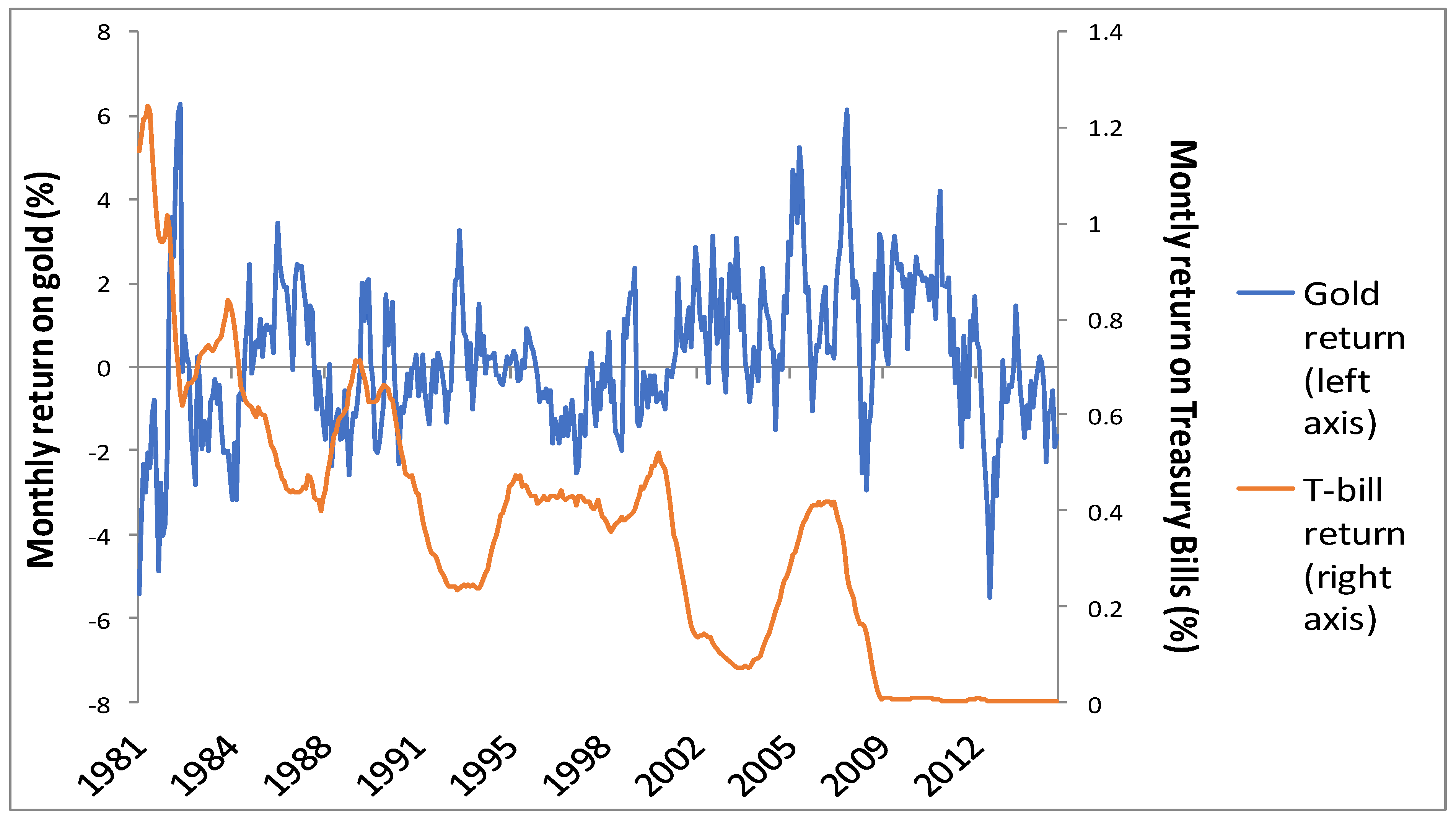
In Figure 1, we use 6-month moving averages of the 1-month returns on gold and Treasury bills to illustrate their trends in different time periods. The returns on gold and Treasury bills have always tended to move in opposite directions, widening during periods of financial crisis, e.g., the stock market crash of 1987, the Mexican peso crisis in 1994, the dot-com bubble in 1993, and the global financial crisis of 2008. This flight-to-safety feature of gold makes it a safe-haven asset during times of market turmoil and crisis, as argued by Baur and Lucey (2010), Baur and McDermott (2010), Kontonikas et al. (2013), and O’Connor et al. (2015).
Market Efficiency Tests: Firstly, we use Lo and MacKinlay (1988) parametric variance-ratio tests and Wright (2000) nonparametric variance-ratio tests to examine the efficiency of gold price series. Results are shown in Table 2, where q shows a number of days, and M1 and M2 show results of the parametric Lo and MacKinlay (1988) test. M1 tests the RWS hypothesis and M2 tests the MDS hypothesis. R1, R2, and S1 are the ranks and signs of the nonparametric test of Wright (2000). R1 and R2 show ranks and test the random walks (RWS), and S1 is the sign that tests the martingale sequence difference hypothesis (MDS). Lo and MacKinlay’s (1988) parametric and Wright’s (2000) nonparametric tests do not reject the null hypotheses of random walks (RWS) and martingale difference sequence (MDS) and confirm the weak-form efficiency of the gold price series.
We further perform the multiple variance-ratio tests of Whang and Kim (2003) using three different time periods (1981–2015, 1990–2015, and 2000–2015) by using six different subsamples. The sampling periods are chosen by using the rule cited in Whang and Kim (2003).3 It allows us to deeply investigate market efficiency, as this procedure allows multiple subsampling to test weak-form efficiency. Results are reported in Table 3 and show that the efficiency of the gold market greatly increased from 2000 onwards. These results are consistent with results of Wang et al. (2011), who found that gold markets achieved greater efficiency after 2000 in the US gold market. This efficiency improves from 1990 onwards and becomes even stronger from 2000 onwards.
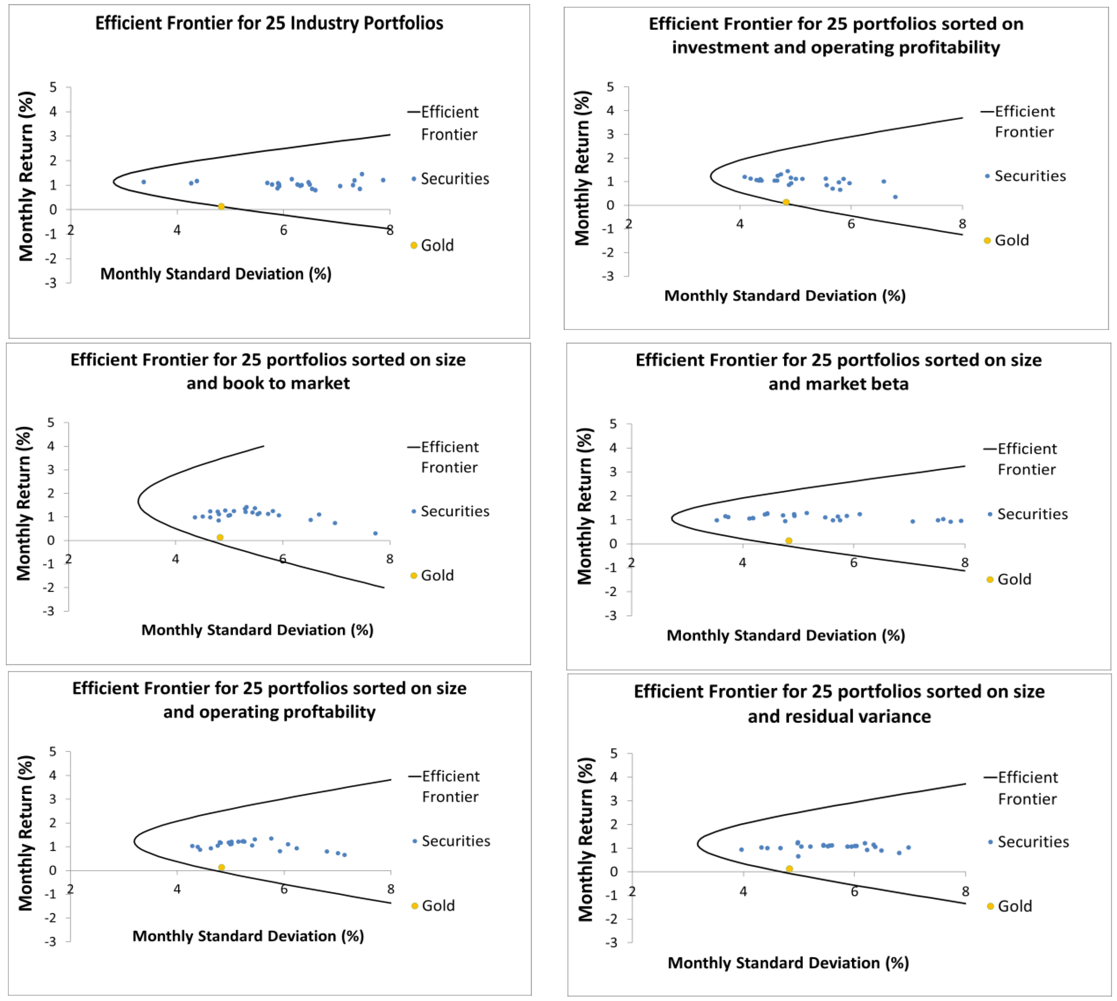
Minimum Variance Efficient Frontier: Gold must be located on minimum variance frontier to satisfy the conditions of Black et al. (1972). Contrary to Treasury bill yield, gold exhibits higher volatility, and this study underlines this limitation and does not attempt to use gold as a risk-free asset.4 Instead, it explores the applicability of gold as a zero-beta asset in a comparative vein of Black et al. (1972). Hence, this study is unique and distinct from Black et al. (1972). However, we still consider the restriction that gold must be located on the efficient frontier to be qualified as a potential zero-beta asset that may replace a risk-free rate or zero-beta portfolio in empirical asset pricing models.
Our study employs the methods of Clarke et al. (2006) and Kan and Smith (2008) to estimate the minimum variance frontier, and our results are presented graphically in Figure 2. The figure illustrates the position of gold on the minimum variance efficient frontier when plotted against various factors, including the 25 industries, the 25 investment and operating profitability, the 25 size and book-to-market, the 25 size and market beta, the 25 size and operating profitability, and the 25 size and residual variance portfolios. Our analysis shows that gold is located close to the minimum variance frontier when plotted against the 25 size and book-to-market, the 25 size and market beta, the 25 size and operating profitability, and the 25 size and residual variance portfolios. However, when plotted against the 25 industries and the 25 investment and operating profitability portfolios, gold is located directly on the minimum variance frontier. These findings suggest that the potential use of gold return as a zero-beta rate warrants further examination to enhance the pricing of industries, investment, and profitability portfolios.
Tests of Factor Models: We begin our analysis by using the returns on the 49 industry portfolios as test assets, since significant industry portfolio exposures to a gold return factor have already been found in the ICAPM framework (Chan and Faff 2002; Davidson et al. 2003). Table 4 and Table 5 report the time-series regression alphas, t-statistics, and R-squared values for the CAPM, three-factor, four-factor, and five-factor models, together with their gold analogues, while Table 6 reports GRS test statistics, the mean-adjusted R-squared, and mean absolute alpha. These results show that first-stage pricing errors are reduced, and R-squared values are substantially improved when gold is used as a zero-beta asset, compared with the conventional models.
We find that gold zero-beta models outperform traditional models, having lower GRS test scores and higher mean-adjusted R-squared values. Wald statistics of the GRS test show that gold is a better proxy of the zero-beta rate than the yield on 1-month T-bills when we apply CAPM and the traditional multifactor models on industry portfolios. Though the single-factor CAPM and G-CAPM, both pass the GRS test at the 5% level, we observe that the gold zero-beta models have a lower number of significant pricing errors compared with the traditional models. For instance, while the single-factor G-CAPM produces four significant pricing errors, the traditional CAPM produces seven. For each model in turn, we obtain fewer significant pricing errors and higher times-series R-squared values by using the gold return in place of the T-bill yield.
Table 7 shows the second-stage Fama and MacBeth (1973) regression results for the 49 industry portfolios. We obtain a positive market risk premium for the G-CAPM with an insignificant cross-sectional alpha, whereas the traditional CAPM produces an implausible negative market risk premium with a significant cross-sectional alpha, showing that the single-factor CAPM improves with gold as a zero-beta asset. While we obtain insignificantly positive market risk premia for both the traditional four-factor model and its gold analogue, we find that the gold model performs better, since it has an insignificant second-stage alpha, whereas that for the conventional model is significant. While the traditional five-factor model performs better than the traditional four-factor model since it has an insignificant alpha with a positive market risk premium, its gold analogue is still superior since it has a higher R-squared. We note that the average cross-sectional R-squared is higher for the single-, three-, four-, and five-factor models when we use gold as a zero-beta asset with industry portfolios.
In unreported results from robustness checks, we also estimate models with Generalized Method of Moments (GMM), adopting the Cochrane (2009) methodology and with Generalized Least Squares (GLS) by using the Kan et al. (2013) procedure. These results are qualitatively similar in terms of demonstrating the advantages of the gold zero-beta asset model and are available from authors on request. Having compared the performance of industry portfolios as test assets, we now move to compare the performance of test portfolios sorted by size and book-to-market ratio.
Table 8 shows the time-series alphas, t-statistics, and R-squared values for the CAPM, three-factor, four-factor, five-factor, and six-factor models and their gold analogues. The comparison of the traditional and the gold zero-beta models shows that pricing errors are reduced, and R-squared values are improved when the gold return is used as a zero-beta asset. Like BJS, we find that gold zero-beta models produce significantly negative alphas for small, low book-to-market portfolios and positive alphas for high book-to-market portfolios.
Table 9 presents a summary of GRS test results for traditional CAPM and gold zero-beta models. We estimate models with (denoted 5 × 5) and without microcaps (denoted 4 × 5) to assess whether our zero-beta models enable us to price smaller stocks, which have been reported as challenging and difficult to price by traditional models (Fama and French 2012). We show results in four pairs of columns, contrasting results from traditional and gold zero-beta models, with and without microcaps. Compared with traditional CAPM models, we obtain higher R-squared and lower Sharpe ratio of alphas with zero-beta models. In particular, for the six-factor model, we find improved performance with the gold zero-beta model, obtaining only four significant pricing errors compared with eight with the traditional model.
Table 10 reports the second-stage cross-sectional results for traditional and gold zero-beta models for portfolios sorted by size and book-to-market. In the cross-sectional analysis, a gold zero-beta six-factor model outperforms, as it produces much lower cross-sectional alphas while having only a marginally smaller R-squared. Fama and French (2012, 2015) find that the four-factor model does a better job in explaining average returns in the US market than other models. We therefore compare the performance of traditional and zero-beta G-four-factor models on different sets of test portfolios.
Table 11, Panel A presents a summary of GRS test results for the traditional and gold zero-beta four-factor models for test assets of 25 portfolios, sorted, respectively, by size and momentum, size and investment, and size and operating profitability. Panel B presents results on sets of 25 portfolios, sorted, respectively, by size and accruals, size and variance, size and residual variance, and size and market beta. Panel C presents results on three sets of 32 portfolios sorted simultaneously by size, book-to-market, and operating profitability, by size, book-to-market, and investment, and by size, operating profitability, and investment, respectively, while Panel D presents results for test assets of 35 portfolios sorted by size and net share issues. We do not report the alpha coefficients, t-statistics, and R-squared values for space reasons but only report the summary statistics, namely the GRS test score, mean-adjusted R-squared, Sharpe ratio of alphas, and number of significant alpha coefficients across all test portfolios. The performance of the zero-beta G-four-factor models remains superior across all test portfolios, since we obtain higher mean-adjusted R-squared values and a lower Sharpe ratio of alphas with gold zero-beta models. Furthermore, the zero-beta G-four-factor models produce fewer significant pricing errors on all test portfolios. However, the traditional and gold zero-beta four-factor model succeeds in passing the GRS test only on the size and book-to-market portfolios, whereas the zero-beta four-factor model produces just two pricing errors compared with five with the traditional four-factor model. As expected, performance is considerably improved when microcaps are omitted for both traditional and zero-beta models.
Table 12 assesses the ability of traditional and zero-beta four-factor models to explain the cross-section of returns on the portfolios explored above. The traditional four-factor model does a reasonable job, as we cannot reject the null hypothesis that second-stage pricing errors are significantly different from zero. In general, for the traditional four-factor model, we obtain an insignificantly positive estimate of the market risk premium and an insignificant cross-sectional alpha. The exceptions are for the 25 size and residual variance portfolios and the 32 size, book-to-market, and investment portfolios, where we find alphas for the traditional model are significant, and the market risk premia are negative, contrary to theory. However, in these instances, we find that the corresponding gold zero-beta model succeeds, having insignificant alphas and a positive estimate of the market risk premium, in line with the theory.
Satisfyingly, we obtained a positive estimate of the market risk premium with the gold zero-beta four-factor model on all test portfolios. The estimate of the market risk premium is significant on the 25 size and momentum and 32 size, book-to-market, and investment portfolios. However, when we exclude microcap portfolios, we obtain insignificantly positive cross-sectional market coefficients. These results are similar and comparable to the traditional four-factor model. We infer from this that employing gold as a zero-beta asset helps to price smaller stocks. Kothari et al. (1995) find that the conclusions made using CAPM tests are sensitive to the time period employed. We therefore perform a subperiod analysis and find that zero-beta models perform better during periods of market uncertainty. The results are not reported, but they are available from the authors on request.
As a robustness test, we derive the orthogonalized gold residual factor, R t G , as above, and include it as a fifth factor in the traditional four-factor model for portfolios sorted by size and momentum in order to test whether the return on gold contains additional explanatory power beyond the four-factor model. Table 13 demonstrates that this residual factor R t G is significant in cross-section and therefore adds significant information beyond the four-factor model in explaining portfolio returns.
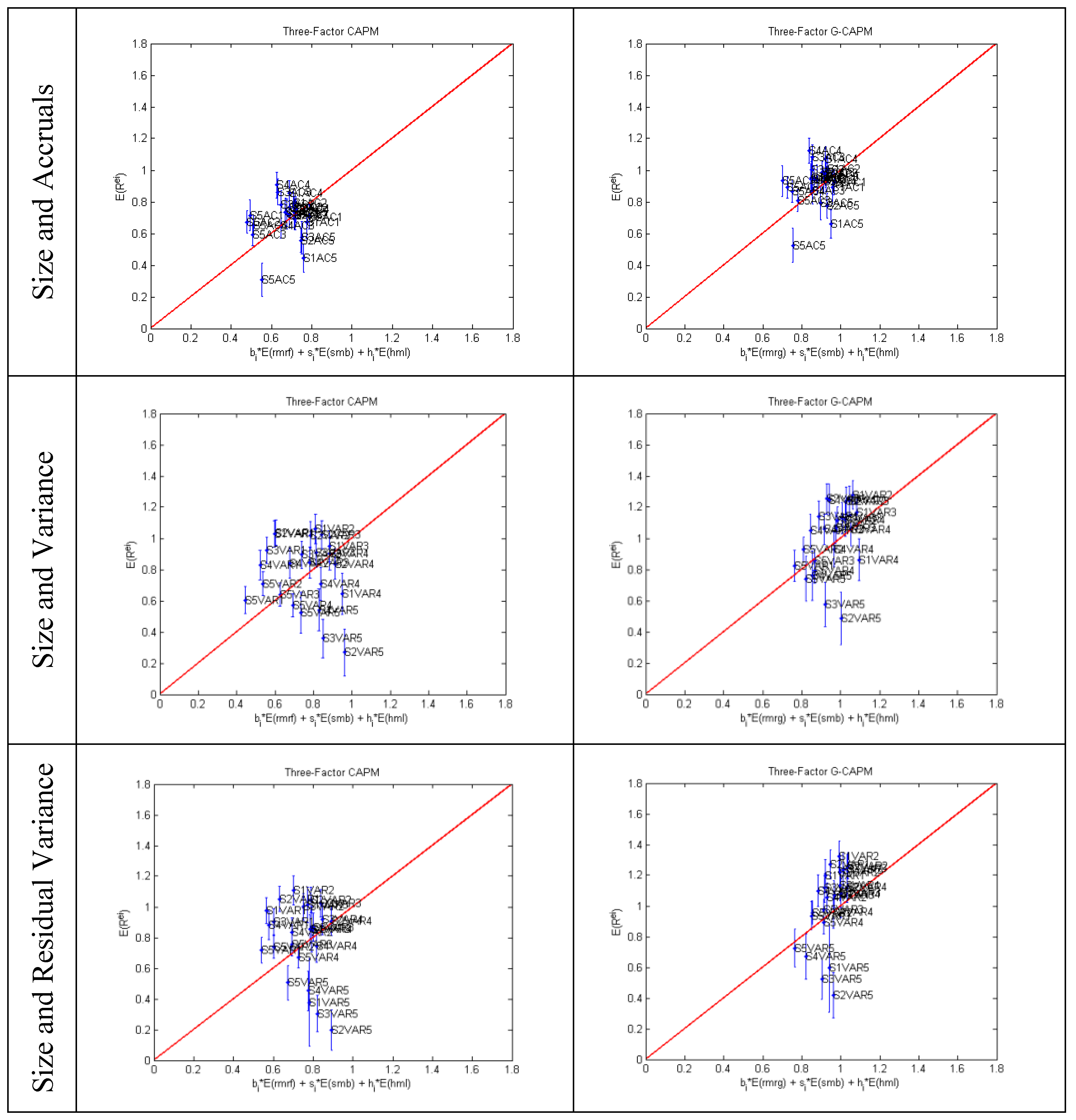
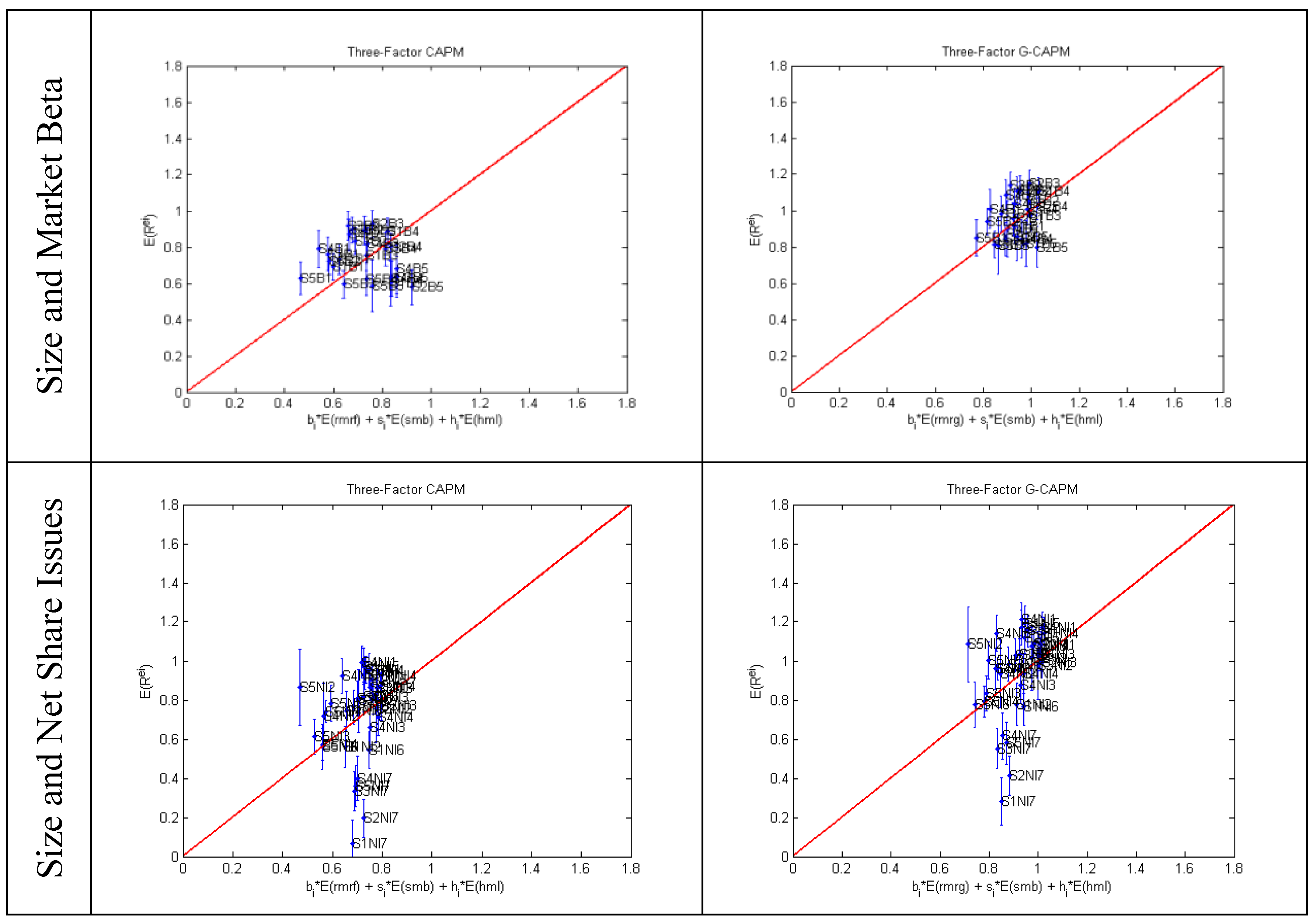
After assessing the performance of the gold zero-beta four-factor model, we assess the performance of the three-factor gold zero-beta model against the traditional three-factor model on test assets of the 25 portfolios sorted, respectively, by size and accruals, by size and variance, by size and residual variance, and by size and market beta, as well as 35 portfolios sorted by size and net share issues. The results of the GRS test in Table 14 show that the gold zero-beta three-factor model produces a lower Sharpe ratio of alphas SR(a) and higher adjusted R-squared values on all test portfolios compared with the traditional three-factor model. The zero-beta three-factor model passes the GRS test at the 5% level on the size and market beta portfolios, whereas the traditional three-factor model fails the GRS test on these assets, with and without microcaps. Furthermore, the zero-beta G-three-factor model produces fewer significant pricing errors on all test portfolios, particularly on portfolios sorted by size and net share issues, whereas it only produces six significant time-series alphas, compared with fifteen with the traditional three-factor model.
Table 15 shows that the gold zero-beta three-factor model performs better in explaining cross-sectional returns than the traditional three-factor model on test portfolios which are not sorted by the Fama–French factors. For the traditional model, we obtain significant cross-sectional alphas for portfolios sorted by size and variance, by size and residual variance, and by size and net share issues at the 5% level. By contrast, the gold zero-beta three-factor model on these test assets yields insignificant cross-sectional alphas. Furthermore, the traditional three-factor model produces an implausibly negative estimate of the market risk premium, whereas the gold zero-beta three-factor model produces an insignificant but economically plausible and positive estimate for all test portfolios, except for those sorted by size and accruals. When we exclude microcaps, we obtain similar and comparable estimates for the traditional and gold zero-beta three-factor models, showing that gold as a zero-beta factor improves the pricing of microcaps in particular. The actual and predicted returns estimated from traditional and zero-beta three-factor models are graphically shown in Figure 3.
We also examine the applicability of gold as a zero-beta asset on the Fama and French (2015) five-factor model. The results are shown in Table 16 in four pairs of columns for comparison, as before. Panel A shows results for test assets of 25 portfolios, sorted by size and momentum, by size and investment, and by size and operating profitability. We find relatively lower Sharpe ratios of alphas SR(a) with the gold zero-beta five-factor model and higher mean-adjusted R-squared values compared with the traditional five-factor model, showing that the gold zero-beta model performs notably better. For instance, for the G-five factor model, we obtain an R-squared of 0.90 on the 25 size and momentum portfolios, as compared with 0.84 for the traditional five-factor model; for the G-five-factor model, we obtain an R-squared of 0.96 on portfolios sorted by size and investment and size and operating profitability, as compared with 0.92 for the traditional five-factor model. In Panel B, the traditional five-factor model produces ten significant alphas for the 32 portfolios sorted by size, book-to-market, and operating profitability, whereas the G-five-factor model produces only seven significant alphas. It also yields a lower Sharpe ratio SR(a) of alphas than the traditional five-factor model. The G-five-factor similarly outperforms the 35 portfolios sorted by size and net share issues.
Table 17 reports the second-stage results for the above regressions and assesses the ability of the traditional and G-five-factor models to explain returns in cross-section. For the traditional five-factor model, we reject the null hypothesis that pricing errors are insignificantly different from zero for the 25 size and investment portfolios at the 5% significance level. In panel B, we likewise reject this null hypothesis for the 32 size, book-to-market, and investment portfolios. We also obtain an implausibly negative estimate of the market risk premium for the traditional five-factor model on the 25 size and momentum, 25 size and investment, and 32 size, book-to-market, and investment portfolios.
The G-five-factor model performs much better: the only portfolio where we can reject the null hypothesis of zero pricing errors at the 5% level is for the 25 size and momentum portfolios. Additionally, we obtain an insignificantly positive estimate of the market risk premium on the 25 size and investment portfolios and a significantly positive estimate for the 25 size and momentum portfolios and for the 32 size, book-to-market, and investment portfolios. In summary, we find that the G-five-factor model does a better job in the portfolios where the traditional five-factor model struggles to explain the cross-section of returns.

6. Conclusions and Areas for Future Research

Our findings indicate that the gold zero-beta models can play a significant role in enhancing the empirical performance of asset pricing models. This study attempts to improve the estimation of expected returns for a wide range of portfolios of US stocks over a 35-year time sample by utilizing gold as a zero-beta asset. We used the price of a fixed weight of gold in lieu of a 1-month T-bill. By using gold returns as a substitute zero-beta rate, we transform all asset prices into units of a fixed weight of gold, as we quote stock prices in terms of ounces of gold rather than quoting in units of Treasury bills. This approach allows for the development of an alternative and parallel technique for estimating stock returns with asset pricing models. Wald statistics of the GRS tests show that gold is a better proxy of the zero-beta rate than the yield on 1-month T-bills when we apply CAPM and the traditional multifactor models on the US industry portfolios and the 25 test portfolios sorted by size and market beta. Overall, empirical findings indicate that asset pricing models employing gold as a zero-beta asset in place of the conventional T-bill risk-free rate have superior time-series and cross-sectional performance.
Our primary findings pertain to the three-factor, four-factor, and five-factor models. For all these, we find that when we use gold as a zero-beta factor in place of the T-bill yield as a risk-free rate, we obtain higher mean-adjusted R-squared values and lower Sharpe ratios of alphas in time series. This indicates that gold as a zero-beta asset improves the time-series performance of traditional empirical factor models. In the second-stage, cross-sectional results, we find that the use of gold as a zero-beta factor brings improvements in two areas. Firstly, our findings suggest that gold as a zero-beta asset can be used to enhance the pricing of smaller stocks, as gold zero-beta models generate economically plausible prices of market risk on test assets, including microcaps, when traditional models with T-bill rates as risk-free assets tend to fail to do so, resulting in negative estimates of the price of market risk. Secondly, we find that using gold as a zero-beta asset reduces the magnitude of pricing errors where traditional models exhibit significant cross-sectional pricing of the intercept.
We also identify the specific test assets on which the gold zero-beta models clearly outperform traditional models. Firstly, the G-four- and five-factor models demonstrate superior performance for portfolios sorted by industry, size, and momentum, as well as for portfolios simultaneously sorted by size, book-to-market, and investment. Secondly, the G-three-factor model performs better for portfolios sorted by size and variance, size and residual variance, and size and market beta. The inclusion of gold as a zero-beta factor in security analysis may provide an alternative estimate for determining whether securities are undervalued or overvalued, and thus may aid investors in making more informed investment decisions. The findings of this research can be valuable for policymakers in making central bank rate-setting decisions and for regulatory bodies in framing appropriate regulations during abrupt market conditions. The use of gold as a zero-beta factor in asset pricing models has the potential to act as a ‘whistleblower’ for regulatory authorities, helping to implement effective policies during periods of financial and economic crises. Subperiod analyses provided improved estimates of market risk; however, these results are not presented in this paper but can be made available upon request from the authors.
In terms of security analysis, utilizing gold as a zero-beta asset may provide an alternative estimate for assessing whether securities are undervalued or overvalued. This can assist investors in making rational investment decisions. Furthermore, utilizing gold as an alternative to the Treasury bill rate may help overcome the empirical weaknesses of factor models during periods of market volatility and uncertainty, as it obtains better estimates of the actual market returns in small and large datasets. The precise estimation of returns made possible through the use of gold zero-beta models can enable investors to assess whether securities are appropriately priced when making investment decisions. Additionally, as mentioned earlier, gold zero-beta models may work as a whistle-blower for regulatory authorities as it can help them to determine the fair return on Treasury bills.
Our paper suggests several potential avenues for future research. Firstly, it is conjectured that gold zero-beta models may be particularly useful during financial crises and pandemics when the risk-free rate, as measured by T-bills, tends to be artificially depressed below the natural risk-free rate as a policy measure. As such, these models may be doubly useful to investors and regulatory authorities during such periods. We strongly argue that gold as a zero-beta asset can be equally useful during periods of pandemics and market volatility, as gold prices swiftly react and adjust prices in response to uncertain market conditions. Secondly, the validity of gold zero-beta models needs to be assessed on markets other than the US to avoid accusations of data snooping, which may arise if only one market is investigated. Thirdly, as recent research suggests that forecasting models can predict future gold prices (Wang et al. 2011; Mihaylov et al. 2015), the findings of this paper open prospects for future research in predicting market booms and crashes. Finally, other statistical modeling techniques, such as neural networks (e.g., Guresen et al. 2011; Khashei and Bijari 2014) and gene expression programming, as well as more conventional econometric modeling methods such as GMM and novel models such as ILCC (Liang et al. 2022), Bidirectional Long Short-Term Memory Network (BiLSTM), Attention Mechanism, Convolutional Neural Network (CNN) (Lin et al. 2022a), and the VMD-AR-IBiLSTM-ELMAN model with asymmetric features and nonlinear integration approach (Lin et al. 2022b) could be applied to assess whether different results are obtained.
It is important to acknowledge the limitations of this study. The use of gold returns as a proxy for the zero-beta rate, rather than a portfolio of risky securities, restricts the generalizability of the results to other assets. However, the study assumes that gold has unique properties that make it a suitable proxy for the zero-beta rate, including its reputation as a safe-haven asset. Despite this, the study cannot claim that gold is a completely risk-free asset, and further research is needed to determine the effectiveness of using gold as a proxy for the risk-free rate across different markets and asset classes. Moreover, the study is limited to the US equity market and may not be generalizable to other regions or markets. Additionally, the study only considers a limited number of test assets and may not account for the full range of asset classes available to investors. Finally, the study’s findings may be sensitive to the time period and sample used, and future research should consider these factors when applying the results.

Author Contributions

Conceptualization, M.A., H.A.A. and C.G.; methodology, M.A, H.A.A. and C.G.; software, M.A and H.A.A.; validation, M.A. and C.G.; formal analysis, M.A.; investigation, M.A., H.A.A. and C.G.; resources, M.A., H.A.A. and A.A.E.; data curation, M.A.; writing—original draft preparation, M.A. and C.G.; writing—review and editing, M.A., H.A.A., A.A.E. and Y.A.; visualization, M.A., H.A.A., A.A.E. and Y.A.; supervision, H.A.A. and C.G. All authors have read and agreed to the published version of the manuscript.

Funding

This research received no external funding.

Informed Consent Statement

Not applicable.

Data Availability Statement

Data available at: Kenneth R. French—Data Library (dartmouth.edu, accessed on 18 December 2022). Gold Prices are obtained from Datastream.

Conflicts of Interest

The authors declare no conflict of interest.

Notes

1
Weil (1990) expands the Kreps–Porteus nonexpected utility preferences (Kreps and Porteus 1978) by separating relative risk aversion and intertemporal substitution.
2
The US owns 8133.5 tons out of 33,604.1 world gold (World Gold Council 2017).
3
We employ six different subsamples (denoted b1, …, b6) for each sample size N: particularly, we use an equally spaced grid having subsample sizes with the range 2.5 × N0.3 < b < 3.5 × N0.6.
4
One of the features of a risk-free asset is that it produces zero variance. However, gold is a volatile asset and is not expected to produce a zero variance. It is used as a zero-beta asset in a comparative vein of Black et al. (1972) when they use a portfolio of risky assets. When risky assets are combined in a single portfolio, the overall variance of a portfolio reduces to a minimum level due to the cumulative effect of variance of individual risky assets (Blume and Friend 1973).

References

  1. Aggarwal, Raj, and Luc A. Soenen. 1988. The Nature and efficency of the gold market. Journal of Portfolio Management 14: 18–21. [Google Scholar] [CrossRef]
  2. Albuquerque, Rui, Martin Eichenbaum, Victor Xi Luo, and Sergio Rebelo. 2016. Valuation Risk and Asset Pricing. The Journal of Finance 71: 2861–904. [Google Scholar] [CrossRef] [Green Version]
  3. Ang, Andrew, Robert J. Hodrick, Yuhang Xing, and Xiaoyan Zhang. 2006. The Cross-Section of Volatility and Expected Returns. The Journal of Finance 61: 259–99. [Google Scholar] [CrossRef] [Green Version]
  4. Bampinas, Georgios, and Theodore Panagiotidis. 2015. Are gold and silver a hedge against inflation? A two century perspective. International Review of Financial Analysis 41: 267–76. [Google Scholar] [CrossRef] [Green Version]
  5. Banz, Rolf W. 1981. The relationship between return and market value of common stocks. Journal of Financial Economics 9: 3–18. [Google Scholar] [CrossRef] [Green Version]
  6. Barberis, Nicholas, Robin Greenwood, Lawrence Jin, and Andrei Shleifer. 2015. X-CAPM: An extrapolative capital asset pricing model. Journal of Financial Economics 115: 1–24. [Google Scholar] [CrossRef] [Green Version]
  7. Barillas, Francisco, and Jay Shanken. 2018. Comparing asset pricing models. The Journal of Finance 73: 715–54. [Google Scholar] [CrossRef] [Green Version]
  8. Barro, Robert J., and Sanjay Misra. 2016. Gold Returns. The Economic Journal 126: 1293–317. [Google Scholar] [CrossRef]
  9. Basu, Sanjoy. 1983. The relationship between earnings’ yield, market value and return for NYSE common stocks. Journal of Financial Economics 12: 129–56. [Google Scholar] [CrossRef]
  10. Baur, Dirk G., and Brian M. Lucey. 2010. Is Gold a Hedge or a Safe Haven? An Analysis of Stocks, Bonds and Gold. Financial Review 45: 217–29. [Google Scholar] [CrossRef]
  11. Baur, Dirk G., and Thomas K. McDermott. 2010. Is gold a safe haven? International evidence. Journal of Banking & Finance 34: 1886–98. [Google Scholar] [CrossRef]
  12. Bekiros, Stelios, Sabri Boubaker, Duc Khuong Nguyen, and Gazi Salah Uddin. 2017. Black swan events and safe havens: The role of gold in globally integrated emerging markets. Journal of International Money and Finance 73: 317–34. [Google Scholar] [CrossRef] [Green Version]
  13. Białkowski, Jędrzej, Martin T. Bohl, Patrick M. Stephan, and Tomasz P. Wisniewski. 2015. The gold price in times of crisis. International Review of Financial Analysis 41: 329–39. [Google Scholar] [CrossRef] [Green Version]
  14. Black, Fischer. 1972. Capital Market Equilibrium with Restricted Borrowing. The Journal of Business 45: 444–55. [Google Scholar] [CrossRef] [Green Version]
  15. Black, Fischer. 1995. Estimating Expected Return. Financial Analysts Journal 51: 168–71. [Google Scholar] [CrossRef]
  16. Black, Fischer, Michael C. Jensen, and Myron. S. Scholes. 1972. The Capital Asset Pricing Model: Some Empirical Tests. In Studies in the Theory of Capital Markets. Edited by Michael C. Jensen. New York: Praeger. [Google Scholar]
  17. Blackburn, Douglas W., and Nusret Cakici. 2017. Overreaction and the cross-section of returns: International evidence. Journal of Empirical Finance 42: 1–14. [Google Scholar] [CrossRef]
  18. Blose, Laurence E. 1996. Gold price risk and the returns on gold mutual funds. Journal of Economics and Business 48: 499–513. [Google Scholar] [CrossRef]
  19. Blose, Laurence E. 2010. Gold prices, cost of carry, and expected inflation. Journal of Economics and Business 62: 35–47. [Google Scholar] [CrossRef]
  20. Blose, Laurence E., and Joseph C. P. Shieh. 1995. The impact of gold price on the value of gold mining stock. Review of Financial Economics 4: 125–39. [Google Scholar] [CrossRef]
  21. Blume, Marshall E., and Irwin Friend. 1973. A new look at the capital asset pricing model. The Journal of Finance 28: 19–34. [Google Scholar] [CrossRef]
  22. Brennan, Michael J. 1971. Capital Market Equilibrium with Divergent Borrowing and Lending Rates. Journal of Financial and Quantitative Analysis 6: 1197–205. [Google Scholar] [CrossRef]
  23. Brennan, Micheal J., Ashley W. Wang, and Yihong Xia. 2004. Estimation and test of a simple model of intertemporal capital asset pricing. The Journal of Finance 59: 1743–75. [Google Scholar] [CrossRef] [Green Version]
  24. Bretscher, Lorenzo, Alex Hsu, Peter Simasek, and Andrea Tamoni. 2020. COVID-19 and the cross-section of equity returns: Impact and transmission. The Review of Asset Pricing Studies 10: 705–41. [Google Scholar] [CrossRef]
  25. Carhart, Mark M. 1997. On persistence in mutual fund performance. The Journal of Finance 52: 57–82. [Google Scholar] [CrossRef]
  26. Carter, Kevin J., John F. Affleck-Graves, and Arthur H. Money. 1982. Are Gold Shares Better than Gold for Diversifiaction? The Journal of Portfolio Management 9: 52–55. [Google Scholar] [CrossRef]
  27. Chan, Howard, and Robert Faff. 2002. The sensitivity of Australian industry equity returns to a gold price factor. Accounting & Finance 38: 223–44. [Google Scholar] [CrossRef]
  28. Chan, Louis K. C., Narasimhan Jegadeesh, and Josef Lakonishok. 1996. Momentum Strategies. The Journal of Finance 51: 1681–713. [Google Scholar] [CrossRef]
  29. Chan, Louis K. C., Yasushi Hamao, and Josef Lakonishok. 1991. Fundamentals and Stock Returns in Japan. The Journal of Finance 46: 1739–64. [Google Scholar] [CrossRef]
  30. Chua, Jess H., Gordon Sick, and Richard S. Woodward. 1990. Diversifying with Gold Stocks. Financial Analysts Journal 46: 76–79. [Google Scholar] [CrossRef]
  31. Ciner, Cetin, Constantin Gurdgiev, and Brian M. Lucey. 2013. Hedges and safe havens: An examination of stocks, bonds, gold, oil and exchange rates. International Review of Financial Analysis 29: 202–11. [Google Scholar] [CrossRef]
  32. Clarke, Roger G., Harindra de Silva, and Steven Thorley. 2006. Minimum-variance portfolios in the US equity market. The Journal of Portfolio Management 33: 10–24. [Google Scholar] [CrossRef]
  33. Cochrane, John H. 2009. Asset Pricing: (Revised Edition). Princeton: Princeton University Press. [Google Scholar]
  34. Cochrane, John H. 2014. Advanced Investments Business 35150. Available online: https://faculty.chicagobooth.edu/john.cochrane/teaching/35150_advanced_investments/ (accessed on 14 November 2017).
  35. Constantinides, George M., and Darrell Duffie. 1996. Asset Pricing with Heterogeneous Consumers. Journal of Political Economy 104: 219–40. [Google Scholar] [CrossRef]
  36. Cui, Moyang, Wing-Keung Wong, Worakamol Wisetsri, Fatma Mabrouk, Iskandar Muda, Zeyun Li, and Marria Hassan. 2023. Do oil, gold and metallic price volatilities prove gold as a safe haven during COVID-19 pandemic? Novel evidence from COVID-19 data. Resources Policy 80: 103133. [Google Scholar] [CrossRef] [PubMed]
  37. Davidson, Sinclair, Robert Faff, and David Hillier. 2003. Gold factor exposures in international asset pricing. Journal of International Financial Markets, Institutions and Money 13: 271–89. [Google Scholar] [CrossRef]
  38. Elsayed, Mohamed, Tamer Elshandidy, and Yousry Ahmed. 2023. Is expanded auditor reporting meaningful? UK evidence. Journal of International Accounting, Auditing and Taxation. Available online: https://pure.qub.ac.uk/en/publications/is-expanded-auditor-reporting-meaningful-uk-evidence (accessed on 18 December 2022).
  39. Fama, Eugene F., and James D. MacBeth. 1973. Risk, return, and equilibrium: Empirical tests. Journal of Political Economy 81: 607–36. [Google Scholar] [CrossRef]
  40. Fama, Eugene F., and Kenneth R. French. 1993. Common risk factors in the returns on stocks and bonds. Journal of Financial Economics 33: 3–56. [Google Scholar] [CrossRef]
  41. Fama, Eugene F., and Kenneth R. French. 1996. Multifactor Explanations of Asset Pricing Anomalies. Journal of Finance 51: 55–84. [Google Scholar] [CrossRef]
  42. Fama, Eugene F., and Kenneth R. French. 2012. Size, value, and momentum in international stock returns. Journal of Financial Economics 105: 457–72. [Google Scholar] [CrossRef]
  43. Fama, Eugene F., and Kenneth R. French. 2015. A five-factor asset pricing model. Journal of Financial Economics 116: 1–22. [Google Scholar] [CrossRef] [Green Version]
  44. Fama, Eugene F., and Kenneth R. French. 2017. International tests of a five-factor asset pricing model. Journal of Financial Economics 123: 441–63. [Google Scholar] [CrossRef]
  45. Fama, Eugene F., and Kenneth R. French. 2018. Choosing factors. Journal of Financial Economics 128: 234–52. [Google Scholar] [CrossRef]
  46. Fama, Eugene F., and Kenneth R. French. 2020. Comparing cross-section and time-series factor models. The Review of Financial Studies 33: 1891–926. [Google Scholar] [CrossRef]
  47. Faria, Joao Ricardo, and Peter McAdam. 2012. A new perspective on the Gold Standard: Inflation as a population phenomenon. Journal of International Money and Finance 31: 1358–70. [Google Scholar] [CrossRef] [Green Version]
  48. Ferguson, Michael. F., and Richard L. Shockley. 2003. Equilibrium “Anomalies”. The Journal of Finance 58: 2549–80. [Google Scholar] [CrossRef]
  49. Fisher, Irving. 1896. Appreciation and Interest: A Study of the Influence of Monetary Appreciation and Depreciation on the Rate of Interest with Applications to the Bimetallic Controversy and the Theory of Interest. Nashville: American Economic Association, vol. 11. [Google Scholar]
  50. Fletcher, Joanthan, and David Forbes. 2002. UK Unit Trust Performance: Does it Matter Which Benchmark or Measure is Used? Journal of Financial Services Research 21: 195–218. [Google Scholar] [CrossRef]
  51. Gibbons, Michael R. 1982. Multivariate tests of financial models: A new approach. Journal of Financial Economics 10: 3–27. [Google Scholar] [CrossRef]
  52. Gibbons, Michael R., Stephen A. Ross, and Jay Shanken. 1989. A Test of the Efficiency of a Given Portfolio. Econometrica 57: 1121–52. [Google Scholar] [CrossRef] [Green Version]
  53. Giglio, Stefano, and Dacheng Xiu. 2021. Asset pricing with omitted factors. Journal of Political Economy 129: 1947–90. [Google Scholar] [CrossRef]
  54. Gil-Alana, Luis A., Goodness C. Aye, and Rangan Gupta. 2015. Trends and cycles in historical gold and silver prices. Journal of International Money and Finance 58: 98–109. [Google Scholar] [CrossRef] [Green Version]
  55. Gospodinov, Nikolay, and Cesare Robotti. 2021. Common pricing across asset classes: Empirical evidence revisited. Journal of Financial Economics 140: 292–324. [Google Scholar] [CrossRef]
  56. Gospodinov, Nikolay, Raymond Kan, and Cesare Robotti. 2013. Chi-squared tests for evaluation and comparison of asset pricing models. Journal of Econometrics 173: 108–25. [Google Scholar] [CrossRef]
  57. Gregory, Alan, Rajesh Tharyan, and Angela Christidis. 2013. Constructing and Testing Alternative Versions of the Fama–French and Carhart Models in the UK. Journal of Business Finance & Accounting 40: 172–214. [Google Scholar]
  58. Guresen, Erkam, Gulgun Kayakutlu, and Tugrul U. Daim. 2011. Using artificial neural network models in stock market index prediction. Expert Systems with Applications 38: 10389–97. [Google Scholar] [CrossRef]
  59. He, Zhen, Fergal O’Connor, and Jacco Thijssen. 2018. Is gold a Sometime Safe Haven or an Always Hedge for equity investors? A Markov-Switching CAPM approach for US and UK stock indices. International Review of Financial Analysis 60: 30–37. [Google Scholar] [CrossRef] [Green Version]
  60. He, Zhen, Fergal O’Connor, and Jacco Thijssen. 2022. Identifying proxies for risk-free assets: Evidence from the zero-beta capital asset pricing model. Research in International Business and Finance 63: 101775. [Google Scholar] [CrossRef]
  61. Hillier, David, Paul Draper, and Robert Faff. 2006. Do Precious Metals Shine? An Investment Perspective. Financial Analysts Journal 62: 98–106. [Google Scholar] [CrossRef]
  62. Ho, Yan-Ki. 1985. A test of the incrementally efficient market hypothesis for the London gold market. Economics Letters 19: 67–70. [Google Scholar] [CrossRef]
  63. Hoang, Thi Hong Van, Hooi Hooi Lean, and Wing Keung Wong. 2015. Is gold good for portfolio diversification? A stochastic dominance analysis of the Paris stock exchange. International Review of Financial Analysis 42: 98–108. [Google Scholar] [CrossRef]
  64. Hou, Kewei, Chen Xue, and Lu Zhang. 2015. Digesting anomalies: An investment approach. The Review of Financial Studies 28: 650–705. [Google Scholar] [CrossRef] [Green Version]
  65. Hou, Kewei, Haitao Mo, Chen Xue, and Lu Zhang. 2018. “Which factors?”. Review of Finance 23: 1–35. [Google Scholar] [CrossRef] [Green Version]
  66. Huang, Darien, and Mete Kilic. 2019. Gold, platinum, and expected stock returns. Journal of Financial Economics 132: 50–75. [Google Scholar] [CrossRef]
  67. Jaffe, Jeffrey F. 1989. Gold and Gold Stocks as Investments for Institutional Portfolios. Financial Analysts Journal 45: 53–59. [Google Scholar] [CrossRef]
  68. Jagannathan, Ravi, and Zhenyu Wang. 1998. An Asymptotic Theory for Estimating Beta-Pricing Models Using Cross-Sectional Regression. The Journal of Finance 53: 1285–309. [Google Scholar] [CrossRef]
  69. Jegadeesh, Narasimhan, and Sheridan Titman. 1993. Returns to Buying Winners and Selling Losers: Implications for Stock Market Efficiency. The Journal of Finance 48: 165–91. [Google Scholar] [CrossRef]
  70. Kan, Raymond, and Daniel R. Smith. 2008. The Distribution of the Sample Minimum-Variance Frontier. Management Science 54: 1364–80. [Google Scholar] [CrossRef] [Green Version]
  71. Kan, Raymond, Cesare Robotti, and Jay Shanken. 2013. Pricing Model Performance and the Two-Pass Cross-Sectional Regression Methodology. The Journal of Finance 68: 2617–49. [Google Scholar] [CrossRef]
  72. Kat, Harry M., and Roel C. A. Oomen. 2006. What Every Investor Should Know About Commodities, Part II: Multivariate Return Analysis. (SSRN Scholarly Paper No. ID 908609). Rochester: Social Science Research Network. Available online: https://papers.ssrn.com/abstract=908609 (accessed on 20 January 2021).
  73. Khashei, Mehdi, and Mehdi Bijari. 2014. Fuzzy artificial neural network (p, d, q) model for incomplete financial time series forecasting. Journal of Intelligent & Fuzzy Systems 26: 831–45. [Google Scholar]
  74. Kontonikas, Alexandros, Ronald MacDonald, and Aman Saggu. 2013. Stock market reaction to fed funds rate surprises: State dependence and the financial crisis. Journal of Banking & Finance 37: 4025–37. [Google Scholar] [CrossRef] [Green Version]
  75. Kothari, Sagar P., Jay Shanken, and Richard G. Sloan. 1995. Another Look at the Cross-section of Expected Stock Returns. The Journal of Finance 50: 185–224. [Google Scholar] [CrossRef]
  76. Kreps, David M., and Evan L. Porteus. 1978. Temporal Resolution of Uncertainty and Dynamic Choice Theory. Econometrica 46: 185–200. [Google Scholar] [CrossRef] [Green Version]
  77. Larsen, Alan B., and Grant R. McQueen. 1995. REITs, real estate, and inflation: Lessons from the gold market. The Journal of Real Estate Finance and Economics 10: 285–97. [Google Scholar] [CrossRef]
  78. Lawrence, Colin. 2003. Why Is Gold Different from Other Assets? An Empirical Investigation. London: The World Gold Council. [Google Scholar]
  79. Lewellen, Jonathan, Stefan Nagel, and Jay Shanken. 2010. A skeptical appraisal of asset pricing tests. Journal of Financial Economics 96: 2175–94. [Google Scholar] [CrossRef] [Green Version]
  80. Liang, Yanhui, Yu Lin, and Qin Lu. 2022. Forecasting gold price using a novel hybrid model with ICEEMDAN and LSTM-CNN-CBAM. Expert Systems with Applications 206: 117847. [Google Scholar] [CrossRef]
  81. Lin, Yu, Kechi Chen, Xi Zhang, Bin Tan, and Qin Lu. 2022a. Forecasting crude oil futures prices using BiLSTM-Attention-CNN model with Wavelet transform. Applied Soft Computing 130: 109723. [Google Scholar] [CrossRef]
  82. Lin, Yu, Qin Lu, Bin Tan, and Yuanyuan Yu. 2022b. Forecasting energy prices using a novel hybrid model with variational mode decomposition. Energy 246: 123366. [Google Scholar] [CrossRef]
  83. Lintner, John. 1965. The Valuation of Risk Assets and the Selection of Risky Investments in Stock Portfolios and Capital Budgets. The Review of Economics and Statistics 47: 13–37. [Google Scholar] [CrossRef]
  84. Lo, Andrew W., and A. Craig MacKinlay. 1988. Stock Market Prices Do Not Follow Random Walks: Evidence from a Simple Specification Test. The Review of Financial Studies 1: 41–66. [Google Scholar] [CrossRef]
  85. Long, Shaobo, Hongxia Pei, Hao Tian, and Kun Lang. 2021. Can both Bitcoin and gold serve as safe-haven assets? A comparative analysis based on the NARDL model. International Review of Financial Analysis 78: 101914. [Google Scholar] [CrossRef]
  86. Low, Rand Kwong Yew, Yiran Yao, and Robert Faff. 2016. Diamonds vs. precious metals: What shines brightest in your investment portfolio? International Review of Financial Analysis 43: 1–14. [Google Scholar] [CrossRef] [Green Version]
  87. Maio, Paulo, and Santa Pedro Clara. 2012. Multifactor models and their consistency with the ICAPM. Journal of Financial Economics 106: 586–613. [Google Scholar] [CrossRef]
  88. Markowitz, Harry M. 1959. Portfolio Selection: Efficient Diversification of Investments. New Haven: Yale University Press. [Google Scholar]
  89. McCown, James Ross, and John R. Zimmerman. 2006. Is Gold a Zero-Beta Asset? Analysis of the Investment Potential of Precious Metals. (SSRN Scholarly Paper No. ID 920496). Rochester: Social Science Research Network. Available online: https://papers.ssrn.com/abstract=920496 (accessed on 1 March 2018).
  90. Mehra, Rajnish, and Edward C. Prescott. 1985. The equity premium: A puzzle. Journal of Monetary Economics 15: 145–61. [Google Scholar] [CrossRef]
  91. Merton, Robert C. 1973. An Intertemporal Capital Asset Pricing Model. Econometrica 41: 867–87. [Google Scholar] [CrossRef]
  92. Mihaylov, George, Chee Seng Cheong, and Ralf Zurbruegg. 2015. Can security analyst forecasts predict gold returns? International Review of Financial Analysis 41 (Suppl. C): 237–46. [Google Scholar] [CrossRef]
  93. Mossin, Jan. 1966. Equilibrium in a Capital Asset Market. Econometrica 34: 768–83. [Google Scholar] [CrossRef]
  94. Neely, Christopher J., David E. Rapach, Jun Tu, and Guofu Zhou. 2014. Forecasting the equity risk premium: The role of technical indicators. Management Science 60: 1772–91. [Google Scholar] [CrossRef] [Green Version]
  95. Nguyen, Duc Binh Benno, Marcel Prokopczuk, and Chardin Wese Simen. 2019. The risk premium of gold. Journal of International Money and Finance 94: 140–59. [Google Scholar] [CrossRef]
  96. Nippani, Srinivas, and Stanley D. Smith. 2010. The increasing default risk of US Treasury securities due to the financial crisis. Journal of Banking & Finance 34: 472–80. [Google Scholar] [CrossRef]
  97. Nippani, Srinivas, Pu Liu, and Craig T. Schulman. 2001. Are Treasury securities free of default? Journal of Financial and Quantitative Analysis 36: 251–65. [Google Scholar] [CrossRef]
  98. Novy-Marx, Robert. 2013. The other side of value: The gross profitability premium. Journal of Financial Economics 108: 11–28. [Google Scholar] [CrossRef] [Green Version]
  99. Ntim, Collins G., John English, Jacinta Nwachukwu, and Yan Wang. 2015. On the efficiency of the global gold markets. International Review of Financial Analysis 41: 218–36. [Google Scholar] [CrossRef]
  100. O’Connor, Fergal A., Brian M. Lucey, Jonathan A. Batten, and Dirk G. Baur. 2015. The financial economics of gold—A survey. International Review of Financial Analysis 41: 186–205. [Google Scholar] [CrossRef]
  101. Pástor, Ľuboš, and Robert F. Stambaugh. 2003. Liquidity risk and expected stock returns. Journal of Political Economy 111: 642–85. [Google Scholar] [CrossRef] [Green Version]
  102. Petkova, Ralitsa. 2006. Do the Fama–French Factors Proxy for Innovations in Predictive Variables? The Journal of Finance 61: 2581–612. [Google Scholar] [CrossRef]
  103. Pierdzioch, Christian, Marian Risse, and Sebastian Rohloff. 2014. On the efficiency of the gold market: Results of a real-time forecasting approach. International Review of Financial Analysis 32 (Suppl. C): 95–108. [Google Scholar] [CrossRef]
  104. Reboredo, Juan C. 2013. Is gold a hedge or safe haven against oil price movements? Resources Policy 38: 2130–37. [Google Scholar] [CrossRef]
  105. Reinganum, Marc R. 1981. A New Empirical Perspective on the Capm. Journal of Financial & Quantitative Analysis 16: 439–62. [Google Scholar]
  106. Shanken, Jay. 1992. On the Estimation of Beta-Pricing Models. The Review of Financial Studies. 5: 1–33. [Google Scholar] [CrossRef]
  107. Sharpe, William F. 1964. Capital Asset Prices: A Theory of Market Equilibrium Under Conditions of Risk*. The Journal of Finance 19: 425–42. [Google Scholar] [CrossRef] [Green Version]
  108. Stambaugh, Robert F., and Yu Yuan. 2016. Mispricing factors. The Review of Financial Studies 30: 1270–315. [Google Scholar] [CrossRef] [Green Version]
  109. Tschoegl, Adrian E. 1980. Efficiency in the gold market—A note. Journal of Banking & Finance 4: 4371–79. [Google Scholar]
  110. Walkshäusl, Christian. 2016. Mispricing and the five-factor model. Economics Letters 147: 99–102. [Google Scholar] [CrossRef]
  111. Wang, Yudong, Yu Wei, and Chongfeng Wu. 2011. Analysis of the efficiency and multifractality of gold markets based on multifractal detrended fluctuation analysis. Physica A: Statistical Mechanics and Its Applications 390: 817–27. [Google Scholar] [CrossRef]
  112. Weil, Philippe. 1989. The equity premium puzzle and the risk-free rate puzzle. Journal of Monetary Economics 24: 401–21. [Google Scholar] [CrossRef]
  113. Weil, Philippe. 1990. Nonexpected Utility in Macroeconomics. The Quarterly Journal of Economics 105: 29–42. [Google Scholar] [CrossRef]
  114. Whang, Yoon-Jae, and Jinho Kim. 2003. A multiple variance ratio test using subsampling. Economics Letters 79: 225–30. [Google Scholar] [CrossRef]
  115. Wiersema, Ubbo F. 2008. Brownian Motion Calculus. New York: John Wiley & Sons. [Google Scholar]
  116. World Gold Council. 2017. Annual Review. Available online: https://www.gold.org/goldhub/research/annual-review-2017 (accessed on 18 December 2022).
  117. Wright, Jonathan H. 2000. Alternative Variance-Ratio Tests Using Ranks and Signs. Journal of Business & Economic Statistics 18: 1–9. [Google Scholar] [CrossRef]
  118. Wu, Chih-Chiang, and Junmao Chiu. 2017. Economic evaluation of asymmetric and price range information in gold and general financial markets. Journal of International Money and Finance 74: 53–68. [Google Scholar] [CrossRef]
Figure 1. 6 month moving averages of the 1-month return on gold and Treasury bills from January 1981 to December 2015.
Jrfm 16 00204 g001
Figure 2. Position of gold on the minimum variance Frontier in the US equity market when it is plotted against the 25 US industries.
Jrfm 16 00204 g002
Figure 3. Comparison of traditional and zero-beta three-factor models. We are grateful to Cochrane (2014) for providing the Matlab codes.
Jrfm 16 00204 g003aJrfm 16 00204 g003b
Table 1. Summary statistics for the returns on gold, market, Treasury bills, Fama–French and Carhart (Momentum) factors from January 1981 to December 2015. Panel A reports average monthly returns, standard deviation, kurtosis, skewness, and t-mean (ratio of the mean to its standard error). Panel B reports correlations among the factor returns. Panel C reports the results of the regression R G , t R F , t = α + β R m , t R F , t + e i , t .
Panel A: Summary Statistics
Rg R g R F R m R F R f SMBHMLMOMRMWCMA
Mean0.14−0.220.600.360.110.340.580.340.33
Std4.834.874.450.282.922.934.492.492.01
Kurtosis1.891.812.420.515.362.3012.1412.992.03
Skewness−0.14−0.15−0.720.700.460.12−1.59−0.470.42
t−mean0.59−0.922.7825.980.762.372.672.823.41
Panel B: Correlations
Rg R g R F R m R F R f SMBHMLMOMRMWCMA
Rg1.00
R g R F 0.991.00
R m R F 0.020.021.00
R f −0.11−0.17−0.061.00
SMB0.060.060.19−0.071.00
HML−0.07−0.08−0.280.11−0.171.00
MOM0.040.03−0.170.050.03−0.191.00
RMW−0.09−0.09−0.340.03−0.440.290.101.00
CMA0.00−0.01−0.400.07−0.070.680.030.151.00
Panel C: Gold beta
Coefficientt-stat
Intercept−0.235−0.979
Rm − RF0.0270.509
Table 2. Variance-ratio test results of daily spot gold price return series: January 1981 to December 2015.
PeriodM1M2R1R2S1
United States
q = 150.890.891.171.021.21
q = 201.000.941.281.101.34
q = 251.091.031.391.191.44 *
q = 301.151.091.48 *1.271.52 *
Note: A test statistic with *, **, and *** indicates significance at the 10%, 5%, and 1% levels, respectively.
Table 3. Multiple variance-ratio tests of the gold price series: January 1981 to December 2015; b1, b2, …, b6 show subsamples of different lengths that increase from b1, b2, …, b6. p-values are reported for the null hypothesis that the gold price series follow a random walk.
b
b1b2b3b4b5b6
Panel A
N = 4174
2000–2015
0.210.250.250.250.220.24
Panel B
N = 6524
1990–2015
0.130.180.250.260.260.26
Panel C
N = 9132
1981–2015
0.030.070.110.150.140.12
Table 4. Alphas from the CAPM, G-CAPM, three-factor, and G-three-factor regressions on 49 industry portfolios from January 1981 to December 2015. The table reports alphas (α), t-statistics t(a), and adjusted R-squared of the tested models.
Return on T-Bills as RfGold as a Zero Beta AssetReturn on T-Bills as RfGold as a Zero Beta Asset
CAPMG-CAPMThree-FactorG-Three-Factor
αt(α)R2αt(α)R2αt(α)R2αt(α)R2
Agriculture0.200.790.300.160.620.550.150.600.320.080.310.56
Food Products0.583.370.370.462.470.680.513.040.410.382.160.72
Candy & Soda0.511.790.260.421.460.530.331.170.290.250.890.55
Beer & Liquor0.653.220.320.542.510.630.663.260.340.522.500.65
Tobacco Products0.812.750.190.712.370.460.702.390.220.602.060.49
Recreation−0.12−0.510.49−0.11−0.460.66−0.23−0.990.52−0.22−0.930.68
Entertainment0.150.640.600.220.920.700.010.030.620.110.450.72
Printing and Publishing−0.02−0.110.66−0.04−0.250.81−0.17−1.040.68−0.17−1.080.82
Consumer Goods0.231.490.530.140.900.770.191.250.540.100.620.78
Apparel0.211.000.550.190.900.730.060.300.570.060.270.74
Healthcare0.040.140.350.040.140.56−0.12−0.450.39−0.12−0.460.58
Medical Equipment0.221.330.580.201.220.760.261.560.580.221.300.77
Pharmaceutical Products0.432.570.490.372.110.730.543.350.540.452.730.76
Chemicals0.050.320.670.090.570.79−0.12−0.770.70−0.04−0.260.81
Rubber and Plastic Products0.150.850.610.150.830.77−0.01−0.040.69−0.01−0.080.82
Textiles0.160.560.440.140.490.63−0.25−1.010.59−0.23−0.960.72
Construction Materials0.020.110.660.050.300.78−0.21−1.260.72−0.13−0.790.81
Construction−0.32−1.470.61−0.21−0.930.69−0.53−2.560.66−0.38−1.770.73
Steel Works Etc−0.55−2.290.62−0.36−1.430.64−0.67−2.910.66−0.45−1.840.68
Fabricated Products−0.51−1.880.41−0.49−1.820.59−0.67−2.700.52−0.67−2.710.66
Machinery−0.22−1.320.73−0.11−0.610.78−0.32−2.000.76−0.18−1.100.81
Electrical Equipment0.130.830.740.201.220.810.110.700.740.211.250.81
Automobiles and Trucks−0.13−0.510.54−0.09−0.350.68−0.46−2.030.62−0.36−1.540.72
Aircraft0.150.740.570.140.700.74−0.01−0.070.590.010.060.75
Shipbuilding, Railroad Equipment0.00−0.010.400.050.170.55−0.26−0.930.45−0.17−0.590.58
Defense0.421.540.230.391.390.470.220.810.260.190.710.50
Precious Metals−0.20−0.370.040.390.910.00−0.26−0.470.050.360.830.02
Non−Metallic and Industrial Metal Mining−0.19−0.630.390.080.270.40−0.40−1.320.43−0.07−0.250.43
Coal−0.39−0.800.20−0.19−0.380.23−0.55−1.130.21−0.32−0.650.24
Petroleum and Natural Gas0.090.410.360.110.500.59−0.07−0.310.40−0.03−0.130.62
Utilities0.332.000.240.211.120.610.181.120.350.040.260.69
Communication0.150.960.620.090.610.810.140.910.630.090.560.81
Personal Services−0.12−0.580.52−0.14−0.670.71−0.23−1.100.54−0.25−1.210.72
Business Services−0.06−0.530.83−0.03−0.260.90−0.02−0.230.86−0.01−0.080.92
Computers−0.18−0.750.59−0.11−0.450.690.100.430.650.140.600.74
Computer Software0.060.240.630.190.720.680.492.380.750.572.740.80
Electronic Equipment−0.15−0.690.67−0.06−0.280.740.100.490.740.160.770.81
Measuring and Control Equipment−0.16−0.810.68−0.05−0.240.740.010.050.760.090.510.81
Business Supplies0.110.680.600.110.620.77−0.07−0.420.64−0.05−0.310.80
Shipping Containers0.221.110.530.211.050.720.110.540.540.110.570.72
Transportation0.080.510.630.040.280.80−0.07−0.430.66−0.09−0.590.82
Wholesale0.040.280.720.040.330.85−0.04−0.300.75−0.04−0.310.87
Retail0.332.080.650.261.690.830.311.970.650.241.520.83
Restaurants, Hotels, Motels0.291.730.560.221.330.770.201.220.570.140.820.78
Banking0.080.460.620.050.270.79−0.26−1.770.76−0.23−1.540.86
Insurance0.201.190.600.150.880.79−0.04−0.300.70−0.05−0.350.84
Real Estate−0.44−1.740.46−0.41−1.620.62−0.78−3.650.62−0.73−3.410.73
Trading0.060.420.780.120.770.84−0.05−0.340.790.040.290.85
Other−0.38−1.820.58−0.38−1.840.74−0.44−2.130.59−0.43−2.080.74
Table 5. Alphas from four-factor, G-four-factor, five-factor, and G-five-factor regressions on 49 industry portfolios from January 1981 to December 2015. The table reports alphas (α), t-statistics t(a), and adjusted R-squared of the tested models.
Return on T-Bills as RfGold as a Zero Beta AssetReturn on T-Bills as RfGold as a Zero Beta Asset
Four FactorG-Four-FactorFive-factorG-Five-Factor
αt(α)R2αt(α)R2αt(α)R2αt(α)R2
Agriculture0.100.390.320.010.040.560.000.010.32−0.09−0.350.56
Food Products0.442.570.420.281.570.720.130.830.520.00−0.030.78
Candy & Soda0.361.270.290.260.910.55−0.01−0.040.32−0.07−0.240.58
Beer & Liquor0.552.690.350.391.860.660.241.260.440.110.550.72
Tobacco Products0.672.260.220.551.860.490.170.580.300.120.410.55
Recreation−0.08−0.330.53−0.08−0.330.69−0.52−2.230.56−0.44−1.890.70
Entertainment0.200.880.640.311.340.730.000.000.620.170.710.72
Printing and Publishing−0.16−0.950.68−0.16−1.000.82−0.36−2.240.70−0.32−2.020.83
Consumer Goods0.140.890.540.020.150.78−0.12−0.820.60−0.21−1.440.82
Apparel0.200.970.580.180.880.75−0.19−0.970.64−0.14−0.700.78
Healthcare−0.23−0.850.39−0.22−0.830.58−0.59−2.350.48−0.50−2.020.64
Medical Equipment0.201.210.580.150.920.770.110.620.590.060.380.77
Pharmaceutical Products0.452.780.550.352.110.770.311.900.570.211.280.79
Chemicals−0.03−0.210.710.060.380.81−0.32−2.000.72−0.15−0.920.81
Rubber and Plastic Products0.040.240.690.030.170.82−0.22−1.340.71−0.18−1.120.83
Textiles0.030.140.620.030.120.75−0.51−2.060.62−0.41−1.680.74
Construction Materials−0.17−1.030.72−0.08−0.470.81−0.51−3.170.75−0.32−1.920.83
Construction−0.53−2.520.66−0.34−1.570.73−0.71−3.410.67−0.43−2.000.73
Steel Works Etc−0.53−2.270.66−0.26−1.080.69−0.47−2.010.67−0.16−0.660.70
Fabricated Products−0.47−1.900.54−0.49−2.000.68−0.74−2.960.55−0.72−2.920.68
Machinery−0.15−0.970.770.000.020.83−0.35−2.090.76−0.12−0.720.81
Electrical Equipment0.120.730.740.251.430.810.020.150.740.201.170.81
Automobiles and Trucks−0.21−0.930.65−0.10−0.440.75−0.46−1.960.62−0.28−1.190.72
Aircraft0.090.440.600.110.550.75−0.27−1.370.62−0.17−0.870.76
Shipbuilding, Railroad Equipment−0.21−0.740.45−0.10−0.350.58−0.72−2.590.50−0.48−1.700.61
Defense0.210.740.260.170.600.50−0.12−0.440.33−0.11−0.400.55
Precious Metals−0.29−0.530.050.451.030.02−0.30−0.520.050.561.270.02
Non−Metallic and Industrial Metal Mining−0.28−0.910.430.110.370.45−0.53−1.700.43−0.02−0.070.43
Coal−0.65−1.300.21−0.35−0.700.24−0.69−1.360.21−0.31−0.630.24
Petroleum and Natural Gas−0.07−0.330.40−0.03−0.130.62−0.23−1.040.41−0.15−0.730.62
Utilities0.080.500.36−0.08−0.490.700.030.190.36−0.17−1.010.71
Communication0.171.100.630.100.650.810.181.120.640.090.550.82
Personal Services−0.34−1.620.55−0.35−1.710.73−0.52−2.590.59−0.49−2.470.75
Business Services 0.00−0.040.860.010.130.92−0.08−0.820.86−0.05−0.440.92
Computers0.311.380.670.341.510.760.472.100.680.462.100.77
Computer Software0.612.910.750.703.340.800.693.310.760.793.820.81
Electronic Equipment0.261.310.750.321.620.820.412.090.770.452.350.83
Measuring and Control Equipment0.070.390.760.170.930.820.070.410.770.191.070.83
Business Supplies0.010.060.650.020.150.80−0.37−2.330.68−0.28−1.770.82
Shipping Containers0.180.890.540.180.890.720.020.080.560.050.230.73
Transportation−0.01−0.040.66−0.04−0.280.82−0.23−1.500.69−0.23−1.520.84
Wholesale−0.06−0.480.75−0.06−0.480.87−0.24−1.990.78−0.20−1.700.88
Retail 0.321.940.650.221.400.830.110.730.690.050.320.85
Restaurants, Hotels, Motels0.221.310.570.140.800.78−0.13−0.850.65−0.17−1.100.83
Banking−0.20−1.290.76−0.15−1.030.86−0.25−1.660.77−0.18−1.210.87
Insurance−0.06−0.400.70−0.06−0.440.84−0.15−1.010.71−0.13−0.900.85
Real Estate−0.61−2.860.64−0.57−2.660.74−0.89−4.090.63−0.79−3.620.74
Trading 0.00−0.020.790.120.740.850.201.400.810.322.140.87
Other−0.39−1.860.59−0.38−1.810.74−0.55−2.570.59−0.50−2.360.74
Table 6. Statistical summary of the GRS test in explaining monthly excess returns over Treasury bills and gold return with 49 industry portfolios from January 1981 to December 2015. Results represent monthly percent returns. The regressions use the CAPM, three-factor, four-factor, and five-factor models to explain excess returns on industry portfolios. The GRS statistic tests the null hypothesis that the alphas of all 49 portfolios are jointly equal to zero. a is the average absolute alpha for a set of time-series regressions of the 49 portfolios; R 2 is the mean-adjusted R-squared; s ( a ) is the mean standard error of the alphas; and S R ( a ) is the average Sharpe ratio of the alphas. The critical values for the GRS statistic are 90%: 1.41; 95%: 1.56; 97.5%: 1.69; 99%: 1.86, and 99.9%: 2.25.
Return on T-Bills as Rf
GRS|a|R2s(a)SR(a)No. of p-Values
(p ≤ 0.05)
CAPM1.240.230.520.220.417
Three-Factor1.820.260.560.210.5012
Four-Factor1.730.240.570.210.508
Five-Factor1.810.320.590.210.5218
Gold as a zero beta asset
GRS|a|R2s(a)SR(a)No. of p-Values
(p ≤ 0.05)
G-CAPM1.180.200.680.220.404
G-Three-Factor1.650.220.710.210.488
G-Four-Factor1.640.200.710.210.484
G-Five-Factor1.740.260.730.210.5011
Table 7. Fama–MacBeth tests on 49 industry portfolios from January 1981 to December 2015. The table reports average coefficients for the CAPM, three-factor, four-factor, five-factor, and six-factor models. Results represent monthly percent returns. The first column reports results with Treasury bills as risk-free assets, whereas the second column reports gold as a zero-beta asset. γ is the average coefficient, t-sh is the t-statistic after correcting for errors-in-variables (Shanken 1992), and R 2 is the average cross-sectional R-squared of the tested models.
Return on T-Bills as RfGold as a Zero Beta Asset
CAPMγt-fmt-shR2γt-fmt-shR2
Intercept0.823.113.110.090.541.691.690.11
γRM−0.15−0.45−0.45 0.350.790.79
Three-Factorγt-fmt-shR2γt-fmt-shR2
Intercept0.541.941.900.200.531.641.620.26
γRM0.230.650.65 0.461.021.01
γSMB−0.56−2.50−2.47 −0.47−2.10−2.08
γHML−0.05−0.28−0.28 −0.05−0.24−0.24
Four-Factorγt-fmt-shR2γt-fmt-shR2
Intercept0.642.232.180.230.541.601.580.30
γRM0.120.340.34 0.450.950.94
γSMB−0.59−2.56−2.52 −0.50−2.37−2.35
γHML−0.06−0.30−0.30 −0.05−0.24−0.24
γMom−0.38−0.75−0.73 −0.14−0.28−0.28
Five-Factorγt-fmt-shR2γt-fmt-shR2
Intercept0.280.880.850.280.491.471.440.33
γRM0.431.151.12 0.471.031.01
γSMB−0.56−2.42−2.36 −0.42−2.02−2.00
γHML−0.22−1.15−1.13 −0.16−0.83−0.83
γCMA−0.18−0.82−0.79 −0.12−0.63−0.62
γRMW0.381.761.71 0.271.401.38
Table 8. Alphas from the CAPM, G-CAPM, three-factor, G-three-factor, four-factor, G-four-factor, five-factor, G-five-factor, six-factor, and G-six-factor regressions on 25 size and book-to-market portfolios from January 1981 to December 2015. The table reports alphas (α), t-statistics t(α), and adjusted R-squared of the tested models.
Return on T-Bills as RfGold as a Zero Beta Asset
αt(α)R2αt(α)R2
Low234HighLow234HighLow234HighLow234HighLow234HighLow234High
CAPMG−CAPM
Small−0.870.060.150.430.44−3.610.270.962.642.600.600.590.660.610.61−0.740.110.160.420.43−2.950.521.012.552.510.660.710.800.780.78
2−0.420.100.310.370.28−2.340.712.372.841.650.730.740.730.720.66−0.320.140.310.350.28−1.700.992.402.731.690.780.840.850.850.80
3−0.240.200.190.320.49−1.541.771.782.613.280.760.820.790.730.68−0.140.230.190.310.48−0.872.011.802.523.260.820.890.890.860.82
4−0.020.090.110.330.21−0.190.980.943.031.410.830.860.790.770.700.050.120.120.320.210.421.301.052.881.420.880.920.890.890.83
Big0.030.090.10−0.030.220.391.120.97−0.251.340.890.870.770.690.620.020.070.06−0.080.200.260.880.52−0.571.200.950.940.890.840.79
Three-FactorG−Three-Factor
Small−0.700.080.060.270.17−5.600.860.873.872.330.890.920.940.930.93−0.650.070.020.210.13−5.120.710.312.891.840.920.950.960.960.96
2−0.240.060.140.13−0.08−3.220.911.982.08−1.190.960.950.930.940.95−0.200.070.120.11−0.06−2.650.991.781.72−0.920.970.970.960.970.97
3−0.020.120.010.050.14−0.321.470.070.651.510.950.900.890.880.870.020.140.010.060.170.201.680.160.721.770.960.950.940.940.93
40.170.00−0.100.10−0.132.17−0.05−1.051.17−1.280.930.880.860.870.850.200.04−0.060.11−0.082.640.41−0.661.29−0.770.960.930.920.940.91
Big0.190.04−0.06−0.34−0.143.670.52−0.73−4.15−1.150.950.890.850.880.810.160.04−0.08−0.33−0.093.180.50−0.93−4.00−0.750.980.950.940.940.89
Four-FactorG−Four-Factor
Small−0.610.070.090.220.20−4.820.791.313.212.690.900.920.940.930.93−0.550.060.040.160.15−4.350.610.552.142.030.920.950.960.960.96
2−0.160.080.150.11−0.07−2.251.252.141.69−1.120.960.950.930.940.95−0.120.090.130.08−0.05−1.671.311.871.28−0.780.970.970.960.970.97
30.020.130.030.070.180.261.510.360.841.850.950.900.890.880.870.060.150.040.070.210.851.770.430.902.150.960.950.940.940.93
40.170.02−0.060.11−0.072.120.27−0.651.30−0.640.930.880.860.870.850.220.07−0.020.12−0.012.730.80−0.211.42−0.080.960.930.930.940.92
Big0.180.03−0.05−0.28−0.043.400.44−0.64−3.39−0.350.950.890.850.890.820.150.03−0.08−0.270.012.840.41−0.91−3.290.070.980.950.940.940.90
Five-FactorG−Five-Factor
Small−0.430.240.050.250.16−3.842.820.773.512.180.920.940.940.930.93−0.400.18−0.010.160.11−3.632.14−0.112.161.460.940.960.970.960.96
2−0.110.000.020.04−0.08−1.510.060.330.67−1.280.960.950.940.940.95−0.070.020.020.02−0.05−0.990.360.340.39−0.790.970.970.970.970.97
30.120.03−0.11−0.090.051.610.36−1.45−1.160.490.950.910.900.900.880.150.08−0.08−0.060.112.120.95−1.03−0.731.130.970.950.950.950.93
40.25−0.18−0.290.02−0.173.20−2.24−3.290.21−1.550.940.900.880.870.850.29−0.08−0.190.05−0.073.81−1.01−2.150.54−0.680.960.940.930.940.91
Big0.12−0.11−0.17−0.370.072.32−1.59−2.04−4.390.580.960.910.860.880.830.09−0.08−0.18−0.340.111.90−1.20−2.13−4.090.910.980.960.940.940.90
Six-FactorG−Six-Factor
Small−0.390.220.080.220.18−3.452.581.113.102.470.920.940.940.930.93−0.360.160.010.130.12−3.281.890.131.741.670.940.960.970.960.96
2−0.070.030.040.03−0.08−0.980.400.670.56−1.220.960.950.940.940.95−0.030.040.040.02−0.05−0.490.680.640.27−0.710.970.970.970.970.97
30.130.04−0.08−0.060.081.810.52−1.07−0.800.860.950.910.900.900.880.170.09−0.05−0.030.142.321.12−0.66−0.381.500.970.950.950.950.93
40.24−0.14−0.240.04−0.123.05−1.77−2.780.43−1.070.940.900.890.870.860.29−0.04−0.150.06−0.023.72−0.53−1.640.75−0.210.960.940.940.940.91
Big0.11−0.10−0.15−0.320.122.29−1.40−1.83−3.870.980.960.910.860.890.830.09−0.07−0.16−0.300.151.85−1.01−1.95−3.621.280.980.960.940.950.91
Table 9. Statistical summary of GRS tests to explain regressions of monthly excess returns over Treasury bills and gold return from January 1981 to December 2015. The regressions use the CAPM, three-factor, four-factor, five-factor, and six-factor models to explain excess returns on 25 size and book-to-market portfolios. The GRS statistic tests the null hypothesis that the alphas of all 25 portfolios are jointly equal to zero. a is the average absolute alpha for a set of regression on the portfolios with (5 × 5) and without microcaps (4 × 5); R 2 is the mean-adjusted R-squared; s ( a ) is the mean standard error of alphas; and S R ( a ) is the average Sharpe ratio of alphas. The critical values for the GRS statistic are 90%: 1.41; 95%: 1.56; 97.5%: 1.69; 99%: 1.86, and 99.9%: 2.25.
Return on T-Bills as RfGold as a Zero-Beta AssetReturn on T-Bills as RfGold as a Zero-Beta Asset
5 × 55 × 54 × 54 × 5
GRS|a|R2s(a)SR(a)NGRS|a|R2s(a)SR(a)NGRS|a|R2s(a)SR(a)GRS|a|R2s(a)SR(a)
p ≤ 0.05p ≤ 0.05
CAPM6.150.240.730.140.6394.510.230.840.140.5493.480.210.760.130.422.860.200.860.130.38
Three-Factor6.000.140.900.080.6384.340.130.950.080.5463.710.110.900.080.443.070.110.950.080.40
Four-Factor5.260.130.910.080.6083.780.120.950.080.5172.980.100.900.080.402.510.100.950.080.37
Five-Factor5.340.140.910.080.62103.770.120.950.080.5183.290.120.910.080.432.740.110.950.080.39
Six-Factor4.970.130.910.080.6083.500.110.950.080.5042.890.110.910.080.412.450.100.950.080.37
Table 10. Fama–MacBeth tests with 25 size and book-to-market portfolios with (5 × 5) and without microcaps (4 × 5) from January 1981–December 2015. Results represent monthly percent returns. The table reports average coefficients for the CAPM, three-factor, four-factor, five-factor, and six-factor models. The first and the third columns report results with return on Treasury bills as risk-free rate, whereas the second and fourth columns report results with gold as a zero-beta asset. γ is the average coefficient, t-fm is the t-statistic from the Fama–MacBeth procedure, t-sh is the Shanken (1992) error-in-variables corrected t-statistic, and R 2 is the average cross-sectional R-squared of the tested models.
Return on T-Bills as RfGold as a Zero Beta AssetReturn on T-Bills as RfGold as a Zero Beta Asset
5 × 55 × 54 × 54 × 5
CAPMγt-fmt-shR2γt-fmt-shR2γt-fmt-shR2γt-fmt-shR2
Intercept1.843.683.580.223.862.772.540.181.312.542.520.232.551.921.870.19
γRM−1.06−1.94−1.90 −2.87−2.00−1.84 −0.54−0.99−0.98 −1.56−1.15−1.12
Three-Factorγt-fmt-shR2γt-fmt-shR2γt-fmt-shR2γt-fmt-shR2
Intercept1.675.505.320.522.793.343.180.511.263.173.120.542.322.402.330.54
γRM−1.02−2.76−2.70 −1.94−2.18−2.09 −0.62−1.40−1.38 −1.46−1.45−1.41
γSMB0.060.400.40 0.070.460.46 0.161.121.12 0.161.111.11
γHML0.362.422.42 0.372.522.51 0.271.861.86 0.271.861.86
Four-Factorγt-fmt-shR2γt-fmt-shR2γt-fmt-shR2γt-fmt-shR2
Intercept0.150.380.300.56−1.28−1.40−1.110.550.140.290.250.570.600.520.490.57
γRM0.551.160.94 2.212.291.84 0.541.050.93 0.290.250.23
γSMB0.100.680.67 0.090.590.57 0.140.950.95 0.161.061.06
γHML0.402.702.64 0.382.572.53 0.312.122.10 0.302.012.00
γMom3.574.873.84 3.095.794.72 2.503.172.77 1.512.352.22
Five-Factorγt-fmt-shR2γt-fmt-shR2γt-fmt-shR2γt-fmt-shR2
Intercept1.775.004.630.632.452.332.200.621.142.952.900.622.652.482.370.61
γRM−1.17−2.82−2.67 −1.66−1.51−1.43 −0.50−1.15−1.13 −1.80−1.62−1.55
γSMB0.161.091.09 0.171.161.16 0.161.121.12 0.161.091.08
γHML0.322.222.21 0.332.252.24 0.271.821.82 0.281.921.92
γCMA−0.27−1.23−1.16 −0.07−0.32−0.30 0.180.640.63 0.120.430.42
γRMW0.643.203.04 0.532.522.42 0.110.480.48 0.100.430.42
Six-Factorγt-fmt-shR2γt-fmt-shR2γt-fmt-shR2γt-fmt-shR2
Intercept0.621.471.420.660.030.020.020.650.150.300.300.651.301.141.120.65
γRM0.060.120.10 0.870.790.65 0.531.010.88 −0.41−0.34−0.32
γSMB0.151.031.02 0.151.041.03 0.130.900.89 0.140.970.97
γHML0.392.702.67 0.382.592.56 0.332.222.20 0.322.202.19
γMom3.215.384.38 2.955.594.66 2.703.523.00 1.772.662.46
γCMA−0.20−0.94−0.78 −0.21−0.93−0.78 −0.04−0.14−0.12 −0.09−0.32−0.30
γRMW0.542.742.34 0.572.722.34 0.311.301.14 0.311.271.19
Table 11. Statistical summary of the GRS test to explain four-factor and G-four-factor regressions from January 1981 to December 2015. The GRS statistic tests the null hypothesis that the alphas of all portfolios are jointly equal to zero. a is the average absolute alpha; R 2 is the mean-adjusted R-squared; s ( a ) is the mean standard error of alphas; and S R ( a ) is the average Sharpe ratio of alphas. The critical values for GRS statistic are 90%: 1.41; 95%: 1.56; 97.5%: 1.69; 99%: 1.86, and 99.9%: 2.25. Panel A shows results on 25 size and momentum, 25 size and investment, and 25 size and operating profitability portfolios. Panel B shows results on 25 size and accruals, 25 size and variance, 25 size and residual variance, and 25 size and market beta portfolios with (5 × 5) and without microcaps (4 × 5). Panel C shows results on 32 size, book-to-market, and operating profitability; 32 size, book-to-market, and investment; and 32 size, operating profitability, and investment portfolios with (5 × 5) and without microcaps (4 × 5). Panel D shows results on 35 size and net share issues portfolios with (5 × 5) and without microcaps (4 × 5).
Return on T-Bills as RfGold as a Zero-Beta AssetReturn on T-Bills as RfGold as Zero-Beta Asset
5 × 55 × 54 × 54 × 5
GRS|a|R2s(a)SR(a)No. of p-ValuesGRS|a|R2s(a)SR(a)No. of p-ValuesGRS|a|R2s(a)SR(a)GRS|a|R2s(a)SR(a)
(p ≤ 0.05)(p ≤ 0.05)
Panel A
25 Size and Momentum3.380.150.900.090.48103.230.150.940.090.47102.570.120.900.090.372.590.140.940.090.37
25 Size and Investment3.770.130.910.080.5173.220.120.950.080.4762.220.110.910.080.351.910.110.950.080.32
25 Size and Operating Profitability2.560.130.900.090.4262.120.110.940.090.3852.100.130.900.090.341.860.110.940.090.32
Panel B
25 Size and Accruals2.660.120.900.090.4372.100.110.940.090.3822.220.120.900.080.351.870.120.940.090.32
25 Size and Variance4.380.220.850.100.55123.900.180.910.110.5272.220.170.850.100.351.760.130.920.100.31
25 Size and Residual Variance2.500.220.850.100.42122.130.180.910.110.38102.130.180.870.090.341.920.140.920.100.32
25 Size and Market Beta1.230.100.880.090.2951.100.080.930.100.2721.350.110.870.090.271.200.080.930.100.25
2 × 4 × 42 × 4 × 44 × 44 × 4
GRS |a|R2s(a)SR(a) GRS |a|R2s(a)SR(a) GRS |a|R2s(a)SR(a) GRS |a|R2s(a)SR(a)
Panel C
32 Size, BM and OP2.830.170.840.110.5192.600.150.900.110.4872.920.130.790.120.362.870.120.880.120.35
32 Size, BM and Inv2.690.140.860.090.49112.190.120.930.090.4492.540.140.820.100.332.090.120.910.100.30
32 Size, OP and Inv3.940.180.860.100.60143.480.160.920.100.56102.710.140.810.110.342.740.130.900.110.34
5 × 75 × 74 × 74 × 7
GRS |a|R2s(a)SR(a) GRS |a|R2s(a)SR(a) GRS |a|R2s(a)SR(a) GRS |a|R2s(a)SR(a)
Panel D: 35 Size and Net Share Issues3.500.160.850.100.5983.000.140.910.100.5472.560.140.840.100.452.260.130.910.100.42
Table 12. Fama–MacBeth tests for four-factor and G-four-factor from January 1981 to December 2015. Results represent monthly percent returns. Panel A shows results on 25 size and momentum, 25 size and investment, and 25 size and operating profitability portfolios. Panel B shows results on 25 size and variance, 25 size and residual variance, and 25 size and market beta portfolios. Panel C shows results on 32 size, book-to-market, and operating profitability; 32 size, book-to-market, and investment; and 32 size, operating profitability, and investment portfolios. Panel D shows results on 35 size and net share issues portfolios. Results for all test portfolios are shown with (5 × 5) and without microcaps (4 × 5); γ is the average coefficient, t-fm is the t-statistics from Fama–MacBeth procedure, t-sh is the Shanken (1992) errors-in-variables corrected t-statistic, and R2 is the average cross-sectional R-Squared of the tested models.
Return on T-Bills as RfGold as a Zero Beta AssetReturn on T-Bills as RfGold as a Zero Beta Asset
Panel A5 × 55 × 54 × 54 × 5
25 Size and Momentum
γt-fmt-shR2γt-fmt-shR2γt-fmt-shR2γt-fmt-shR2
Intercept−0.05−0.09−0.090.65−3.99−2.36−1.790.640.711.441.420.65−0.42−0.26−0.250.64
γRM0.691.251.20 4.852.822.17 −0.03−0.06−0.06 1.310.820.78
γSMB0.110.720.71 0.080.510.48 0.171.151.14 0.150.960.95
γHML0.761.971.88 1.113.062.41 0.330.980.97 0.501.521.47
γMom0.683.043.03 0.713.183.15 0.522.342.34 0.552.442.43
25 Size and Investment
γt-fmt-shR2γt-fmt-shR2γt-fmt-shR2γt-fmt-shR2
Intercept0.100.240.220.55−1.12−0.99−0.910.530.621.491.450.562.331.811.750.56
γRM0.551.201.12 2.011.701.56 0.040.090.08 −1.46−1.10−1.06
γSMB0.070.470.47 0.050.360.36 0.090.590.59 0.110.720.72
γHML0.683.463.30 0.683.483.33 0.542.792.77 0.432.182.15
γMom1.632.382.19 1.031.721.58 0.480.700.68 −0.20−0.32−0.31
25 Size and Operating Profitability
γt-fmt-shR2γt-fmt-shR2γt-fmt-shR2γt-fmt-shR2
Intercept0.060.150.130.51−0.87−0.88−0.800.490.461.030.940.530.460.400.370.52
γRM0.571.201.09 1.751.691.53 0.180.360.34 0.410.340.33
γSMB0.060.390.39 0.050.370.37 0.120.810.81 0.130.900.89
γHML0.712.872.62 0.602.602.43 0.552.272.14 0.482.041.97
γMom2.072.652.35 1.582.191.99 1.752.462.27 1.321.781.69
Panel B
25 Size and Accruals
γt-fmt-shR2γt-fmt-shR2γt-fmt-shR2γt-fmt-shR2
Intercept0.451.181.040.480.300.300.280.460.571.491.310.470.870.860.790.46
γRM0.270.570.51 0.630.580.54 0.130.270.24 0.030.030.03
γSMB0.100.620.61 0.090.570.56 0.150.990.97 0.171.131.12
γHML0.240.750.67 0.180.560.53 0.120.420.38 0.010.030.03
γMom2.453.352.96 1.712.432.27 2.422.782.46 1.862.192.04
25 Size and Variance
γt-fmt-shR2γt-fmt-shR2γt-fmt-shR2γt-fmt-shR2
Intercept0.060.260.210.70−1.75−2.29−1.800.680.571.081.070.450.470.450.440.43
γRM0.571.791.58 2.633.132.52 0.080.150.15 0.400.360.36
γSMB0.543.172.96 0.533.152.91 0.231.531.53 0.231.511.51
γHML0.552.141.84 0.492.001.68 0.261.581.57 0.271.651.64
γMom2.944.703.90 0.150.230.23 0.090.150.15
25 Size and Residual Variance
γt-fmt-shR2γt-fmt-shR2γt-fmt-shR2γt-fmt-shR2
Intercept0.582.572.470.720.400.520.500.71−0.06−0.19−0.150.70−1.01−1.12−0.930.68
γRM−0.01−0.03−0.03 0.420.490.48 0.721.841.50 1.931.971.67
γSMB0.231.371.35 0.231.361.34 0.533.012.68 0.422.422.26
γHML0.762.752.67 0.692.642.58 0.481.721.38 0.391.461.27
γMom0.380.570.55 0.390.590.57 3.614.003.08 2.523.272.76
25 Size and Market Beta
γt-fmt-shR2γt-fmt-shR2γt-fmt-shR2γt-fmt-shR2
Intercept0.060.200.190.61−0.62−0.81−0.770.600.110.290.260.63−0.14−0.16−0.150.63
γRM0.591.601.52 1.511.841.75 0.561.311.20 1.051.101.04
γSMB0.110.740.73 0.090.580.57 0.171.101.09 0.161.051.05
γHML0.351.060.99 0.361.101.05 0.160.500.46 0.150.460.44
γMom1.602.732.56 1.011.451.38 2.092.952.68 1.331.941.84
Return on T-Bills as RfGold as a Zero Beta AssetRetusrn on T-Bills as RfGold as a Zero Beta Asset
2 × 4 × 42 × 4 × 44 × 44 × 4
32 Size, Book to Market and Operating Profitability
γt-fmt-shR2γt-fmt-shR2γt-fmt-shR2γt-fmt-shR2
Intercept0.360.710.690.46−1.78−1.86−1.660.440.290.280.260.491.660.910.870.46
γRM0.270.490.48 2.642.632.37 0.380.370.36 −0.74−0.40−0.39
γSMB0.060.440.44 0.060.380.38 0.130.240.23 0.461.020.98
γHML0.462.902.88 0.483.113.05 0.170.960.94 0.130.730.72
γMom0.951.631.58 1.111.901.72 1.361.741.66 0.961.251.20
32 Size, Book to Market and Investment
γt-fmt-shR2γt-fmt-shR2γt-fmt-shR2γt-fmt-shR2
Intercept1.403.513.380.460.730.630.590.451.452.412.320.412.131.291.230.41
γRM−0.76−1.68−1.63 0.140.120.11 −0.72−1.17−1.13 −1.20−0.72−0.69
γSMB0.151.021.02 0.140.970.97 0.461.111.07 0.370.930.89
γHML0.271.861.85 0.302.062.06 0.050.320.32 0.060.360.36
γMom0.921.531.48 1.612.892.73 0.771.091.05 0.981.491.43
32 Size, Investment and Operating Profitability
γt-fmt-shR2γt-fmt-shR2γt-fmt-shR2γt-fmt-shR2
Intercept0.351.090.960.44 −0.68−0.79−0.700.360.840.800.400.580.530.510.40
γRM0.290.750.68 1.541.681.500.240.520.50 0.250.220.21
γSMB0.020.150.15 0.040.250.25−0.51−1.50−1.44 −0.36−1.06−1.04
γHML0.663.693.52 0.623.463.290.261.301.27 0.190.930.91
γMom2.154.894.44 1.934.524.111.102.092.01 0.891.771.73
Panel D
Return on T-Bills as RfGold as a Zero Beta AssetReturn on T-Bills as RfGold as a Zero Beta Asset
5 × 75 × 74 × 74 × 7
35 Size and Net Share
γt-fmt-shR2γt-fmt-shR2γt-fmt-shR2γt-fmt-shR2
Intercept0.270.740.620.44−0.13−0.17−0.150.440.631.491.290.431.001.151.040.44
γRM0.410.950.82 1.051.261.12 0.050.110.10 −0.10−0.11−0.10
γSMB0.040.290.28 0.030.230.22 0.070.500.49 0.110.720.71
γHML0.582.662.38 0.482.272.11 0.431.941.78 0.331.491.41
Table 13. Fama–MacBeth test on 25 size and momentum portfolios with the five-factor model. Results represent monthly percent returns from January 1981 to December 2015. The first four factors are the cross-sectional pricings of the four factors of the Carhart (1997) four-factor model, and γRES is the pricing of R t G , the orthogonalized portion of the gold return against the Carhart four factors. t-sh represents the Shanken (1992) error-in-variables corrected t-statistics. We adopt the Ferguson and Shockley (2003) methodology to derive this factor, adding the alpha and the residual from the time-series regression: R t G o l d = a 0 + a 1 R t M k t R F + a 2 R t S M B + a 3 R t H M L + a 4 R t M O M .
Γ0γRMγSMBγHMLγMOMγRESR2
γ−0.921.600.060.990.71−4.390.67
t-fm−1.502.530.392.533.17−3.35
t-sh−1.041.800.361.813.11−2.33
Table 14. Statistical summary of GRS tests to explain the three-factor and G-three-factor regressions from January 1981 to December 2015. The GRS statistic tests the null hypothesis that the alphas of all portfolios are jointly equal to zero. a is the average absolute alpha; R 2 is the mean-adjusted R-squared; s ( a ) is the mean standard error of alphas; and S R ( a ) is the average Sharpe ratio of alphas. The critical values for the GRS statistic are 90%: 1.41; 95%: 1.56; 97.5%: 1.69; 99%: 1.86, and 99.9%: 2.25. Panel A shows results on 25 size and variance, 25 size and residual variance, 25 size and market beta portfolios, and Panel B shows results on 35 size and net share issues portfolios with (5 × 5) and without microcaps (4 × 5).
Return on t-Bills as RfGold as a Zero-Beta AssetReturn on T-Bills as RfGold as a Zero-Beta Asset
5 × 55 × 54 × 54 × 5
GRS |a|R2s(a)SR(a)No. of p-ValuesGRS|a|R2s(a)SR(a)No. of p-Values GRS |a|R2s(a)SR(a)GRS|a|R2s(a)SR(a)
(p ≤ 0.05)(p ≤ 0.05)
Panel A
25 Size and Accruals3.120.120.900.080.4692.370.120.940.090.4072.500.110.900.080.362.020.110.940.080.32
25 Size and Variance5.050.280.840.100.58124.240.210.900.110.5392.680.220.850.100.381.630.160.910.110.29
25 Size and Residual Variance2.780.230.840.110.43132.050.180.900.110.3792.760.210.860.090.382.140.170.920.100.33
25 Size and Market Beta1.630.150.870.090.33131.320.100.920.100.30101.940.160.870.090.321.540.110.920.100.28
5 × 75 × 74 × 74 × 7
GRS |a|R2s(a)SR(a) GRS |a|R2s(a)SR(a) GRS |a|R2s(a)SR(a) GRS |a|R2s(a)SR(a)
Panel B
35 Size and Net Share Issues3.500.160.850.100.59153.000.140.910.100.5462.560.140.840.100.452.260.130.910.100.42
Table 15. Fama–MacBeth tests for three-factor and G-three-factor model from January 1981 to December 2015. Results represent monthly percent returns. Panel A shows results on 25 size and accruals, 25 size and variance, 25 size and residual variance, and 25 size and market beta portfolios, and Panel B shows results on 35 size and net share issues portfolios with (5 × 5) and without microcaps (4 × 5); γ is the average coefficient, t-fm is the t-statistics from Fama–MacBeth procedure, t-sh is the Shanken (1992) errors-in-variables corrected t-statistic, and R2 is the average cross-sectional R-squared of the tested models.
Return on T-Bills as RfGold as a Zero Beta AssetReturn on T-Bills as RfGold as a Zero Beta Asset
5 × 55 × 54 × 54 × 5
Panel A:γ t-shR2γ t-shR2γ t-shR2γ t-shR2
25 Size and Accruals
1.013.123.100.451.851.841.820.431.083.173.150.432.272.512.450.41
−0.33−0.80−0.80 −0.97−0.89−0.88 −0.43−1.02−1.02 −1.42−1.45−1.42
0.050.350.35 0.060.410.41 0.130.850.85 0.150.960.96
0.200.620.61 0.150.460.46 0.040.160.16 −0.03−0.10−0.10
25 Size and Variance
γt-fmt-shR2γt-fmt-shR2γt-fmt-shR2γt-fmt-shR2
Intercept0.573.082.940.62−0.09−0.14−0.130.610.661.541.530.420.750.680.670.40
γRM0.030.120.11 0.911.281.22 −0.01−0.02−0.02 0.120.100.10
γSMB−0.17−1.00−0.99 −0.18−1.07−1.06 0.231.531.53 0.231.521.52
γHML0.893.263.15 0.903.453.32 0.261.561.56 0.261.601.59
25 Size and Residual Variance
γt-fmt-shR2γt-fmt-shR2γt-fmt-shR2γt-fmt-shR2
Intercept0.532.152.060.620.350.440.420.620.612.492.400.660.831.121.090.65
γRM0.030.080.08 0.450.520.51 −0.04−0.13−0.13 −0.02−0.03−0.03
γSMB0.070.400.39 0.070.410.40 0.090.590.59 0.120.750.75
γHML0.882.972.88 0.812.992.90 0.782.812.74 0.702.682.63
25 Size and Market Beta
γt-fmt-shR2γt-fmt-shR2γt-fmt-shR2γt-fmt-shR2
Intercept0.461.681.650.590.210.280.270.580.722.452.430.610.851.051.050.60
γRM0.160.480.48 0.650.800.78 −0.07−0.19−0.19 0.030.030.03
γSMB0.040.260.26 0.040.270.27 0.090.610.61 0.090.620.62
γHML0.591.741.71 0.551.771.74 0.361.071.06 0.361.071.06
Panel B: 35 Size and Net Share Issues
5 × 75 × 74 × 74 × 7
γt-fmt-shR2γt-fmt-shR2γt-fmt-shR2γt-fmt-shR2
Intercept0.772.442.380.400.640.890.870.411.223.403.340.391.812.242.190.40
γRM−0.12−0.32−0.32 0.230.300.29 −0.56−1.36−1.34 −0.95−1.09−1.07
γSMB0.020.140.14 0.020.120.12 0.110.750.74 0.110.750.75
γHML0.612.772.74 0.632.922.88 0.381.741.72 0.401.811.79
Table 16. Statistical summary of the GRS test to explain five-factor and G-five-factor regressions from January 1981 to December 2015. The GRS statistic tests the null hypothesis that the alphas of all portfolios are jointly equal to zero. a is the average absolute alpha; R 2 is the mean-adjusted R-squared; s ( a ) is the mean standard error of alphas; and S R ( a ) is the average Sharpe ratio of alphas. The critical values for GRS statistic are 90%: 1.41; 95%: 1.56; 97.5%: 1.69; 99%: 1.86, and 99.9%: 2.25. Panel A shows results on 25 size and momentum, size and investment, 25 size and operating profitability with (5 × 5) and without microcaps (4 × 5), Panel B shows results on 32 size, book-to-market, and operating profitability and 32 size, book-to-market, and investment portfolios with (5 × 5) and without microcaps (4 × 5), and Panel C shows results on 35 size and net share issues portfolios with (5 × 5) and without microcaps (4 × 5).
Return on T-Bills as RfGold as a Zero-Beta AssetReturn on T-Bills as RfGold as a Zero-Beta Asset
Panel A5 × 55 × 54 × 54 × 5
GRS |a|R2S(a)SR(a)No. of p-Values GRS |a|R2S(a)SR(a)No. of p-Values GRS |a|R2S(a)SR(a) GRS |a|R2S(a)SR(a)
(p ≤ 0.05)(p ≤ 0.05)
25 Size and Momentum3.470.240.840.120.50103.490.200.900.120.4992.750.210.840.120.392.910.170.900.120.40
25 Size and Investment3.130.090.930.070.4752.820.090.960.070.4451.750.070.920.070.321.660.070.960.070.30
25 Size and Operating Profitability2.410.080.920.080.4242.110.080.960.080.3841.690.070.920.070.311.650.080.960.070.30
Panel B2 × 4 × 42 × 4 × 4 4 × 44 × 4
GRS |a|R2S(a)SR(a) GRS |a|R2S(a)SR(a) GRS |a|R2S(a)SR(a) GRS |a|R2S(a)SR(a)
32 Size, BM and OP2.880.150.850.110.52102.770.150.910.110.5073.110.180.810.120.373.290.170.890.120.38
32 Size, BM and Inv2.410.120.880.090.4852.110.100.940.090.4452.340.140.830.100.322.140.120.920.100.31
Panel C5 × 75 × 7 4 × 74 × 7
GRS |a|R2S(a)SR(a) GRS |a|R2S(a)SR(a) GRS |a|R2S(a)SR(a) GRS |a|R2S(a)SR(a)
35 Size and Net Share Issues3.180.130.860.100.5792.840.140.920.100.5392.240.130.850.100.432.110.130.920.100.41
Table 17. Fama–MacBeth tests for five-factor and G-five-factor model from January 1981 to December 2015. Results represent monthly percent returns. γ is the average coefficient, t-fm is the t-statistics from Fama–MacBeth procedure, t-sh is the Shanken (1992) errors-in-variables corrected t-statistic, and R 2 is the average cross-sectional R-squared of the tested models. Panel A shows results on 25 size and momentum, size and investment and 25 size and operating profitability portfolios, Panel B shows results on 32 size, book-to-market, and operating profitability; 32 size, book-to-market and investment portfolios; and 32 size, operating profitability and investment portfolios, and Panel C shows results on 35 size and net share issues portfolios. All results are shown with (5 × 5) and without microcaps (4 × 5).
Return on T-Bills as RfGold as a Zero Beta AssetReturn on T-Bills as RfGold as a Zero Beta Asset
γ t-shR2γ t-shR2γ t-shR2γ t-shR2
Panel A5 × 55 × 54 × 54 × 5
25 Size and Momentum
γt-fmt-shR2γt-fmt-shR2γt-fmt-shR2γt-fmt-shR2
Intercept0.701.711.650.68−3.33−2.51−1.980.670.822.011.930.68−0.45−0.34−0.320.67
γRM0.00−0.01−0.01 4.263.132.49 −0.14−0.32−0.31 1.350.980.92
γSMB0.231.541.53 0.241.591.54 0.221.441.43 0.211.391.38
γHML−0.54−1.73−1.67 −0.45−1.50−1.24 −0.52−1.46−1.41 −0.55−1.54−1.46
γCMA0.080.270.26 0.672.602.11 −0.14−0.37−0.36 −0.02−0.06−0.06
γRMW0.522.132.06 0.461.911.58 0.521.671.61 0.591.831.73
25 Size and Investment
γt-fmt-shR2γt-fmt-shR2γt-fmt-shR2γt-fmt-shR2
Intercept0.712.102.040.620.250.220.220.600.712.021.980.622.121.741.670.61
γRM−0.07−0.19−0.18 0.610.510.50 −0.07−0.16−0.16 −1.24−0.99−0.95
γSMB0.100.670.66 0.090.620.62 0.130.840.84 0.090.620.62
γHML0.321.071.05 0.341.151.12 0.280.900.88 0.531.681.62
γCMA0.333.183.17 0.323.073.06 0.262.452.45 0.252.332.32
γRMW0.321.271.24 0.311.301.27 0.341.321.30 0.050.190.18
25 Size and Operating Profitability
γt-fmt-shR2γt-fmt-shR2γt-fmt-shR2γt-fmt-shR2
Intercept0.501.191.180.591.691.851.810.560.380.860.850.621.921.851.810.56
γRM0.150.310.31 −0.80−0.83−0.81 0.260.540.53 −1.04−0.83−0.81
γSMB0.030.190.19 0.020.160.16 0.060.440.44 0.080.160.16
γHML0.261.291.28 0.190.990.98 0.190.900.89 0.130.990.98
γCMA−0.01−0.06−0.06 −0.18−0.97−0.96 0.010.030.03 −0.15−0.97−0.96
γRMW0.322.582.57 0.322.542.54 0.312.422.41 0.292.542.54
Return on T-Bills as RfGold as a Zero Beta AssetReturn on T-Bills as RfGold as a Zero Beta Asset
Panel B2 × 4 × 42 × 4 × 44 × 44 × 4
32 Size, Book to Market and Operating Profitability
γt-fmt-shR2γt-fmt-shR2γt-fmt-shR2γt-fmt-shR2
Intercept0.130.240.230.51−1.79−1.68−1.540.511.311.421.370.573.791.981.770.56
γRM0.450.790.77 2.582.332.15 −0.61−0.68−0.66 −2.87−1.50−1.34
γSMB0.110.790.79 0.110.740.73 0.661.251.21 0.721.281.15
γHML0.322.132.12 0.332.152.13 0.080.470.47 0.020.120.12
γCMA−0.02−0.11−0.11 −0.03−0.20−0.19 −0.05−0.23−0.23 0.000.000.00
γRMW0.312.312.31 0.322.402.37 0.080.450.44 0.080.490.46
32 Size, Book to Market and Investment
γt-fmt-shR2γt-fmt-shR2γt-fmt-shR2γt-fmt-shR2
Intercept1.152.942.860.50−0.24−0.21−0.200.501.061.691.640.480.260.130.130.48
γRM−0.55−1.27−1.24 1.020.870.84 −0.34−0.52−0.51 0.670.340.33
γSMB0.181.261.26 0.201.381.38 0.601.031.00 0.510.890.86
γHML0.211.461.46 0.191.281.27 −0.02−0.12−0.11 −0.03−0.17−0.17
γCMA0.272.702.69 0.282.702.70 0.221.911.89 0.232.001.99
γRMW0.311.661.63 0.442.492.44 −0.09−0.31−0.30 −0.09−0.29−0.28
25 Size and Net Share Issues
Panel C5 × 75 × 74 × 74 × 7
γt-fmt-shR2γt-fmt-shR2γt-fmt-shR2γt-fmt-shR2
Intercept0.381.151.120.48−0.46−0.57−0.540.480.571.421.400.480.650.680.660.49
γRM0.270.670.66 1.361.561.50 0.100.210.21 0.240.230.23
γSMB0.100.670.67 0.080.530.52 0.130.870.86 0.140.910.91
γHML0.030.140.14 0.030.120.11 −0.12−0.45−0.45 −0.11−0.39−0.38
γCMA0.251.351.33 0.301.561.51 0.281.281.26 0.261.131.11
γRMW0.412.052.02 0.381.861.81 0.311.371.35 0.311.331.31
Disclaimer/Publisher’s Note: The statements, opinions and data contained in all publications are solely those of the individual author(s) and contributor(s) and not of MDPI and/or the editor(s). MDPI and/or the editor(s) disclaim responsibility for any injury to people or property resulting from any ideas, methods, instructions or products referred to in the content.

