
Stock Portfolio Management by Using Fuzzy Ensemble Deep Reinforcement Learning Algorithm

Abstract
:1. Introduction
2. Methodology
2.1. Model Terminology and Assumptions
- Reward, denoted by r, is a scalar feedback to reflect the performance of actions. The goal of most RL algorithms is to optimize the cumulative reward. For the stock trading problem, it depends on the current market and portfolio information and the trading actions taken, and, therefore, it is denoted as , meaning the change in the total portfolio value when facing state and taking action , and, therefore, the arriving state , where and are defined later in this section.
- We consider a pool of M stocks over T time periods and assume a trader may buy or sell stocks but may not short sell. For each stock i, and time t, where and , let be the price and be the numbers of share holding in the trader’s portfolio. Respectively, combining and yields and . Then, the portfolio’s return at time t iswhere is the transaction cost rate, usually ranging from to . Therefore, our objective is to maximize the total return, the sum of period-wise returns over all periods.
- We define s as the environment state space vector, which will be the model input. In our problem, the environment state space includes two types of components: the quantities that are dependent on trading actions, e.g., account cash balance and stock shareholdings, which is denoted by vector ; and the quantities that are independent of trading actions, e.g., stock prices and technical indicators, such as MACD, denoted by vector . Thus, .
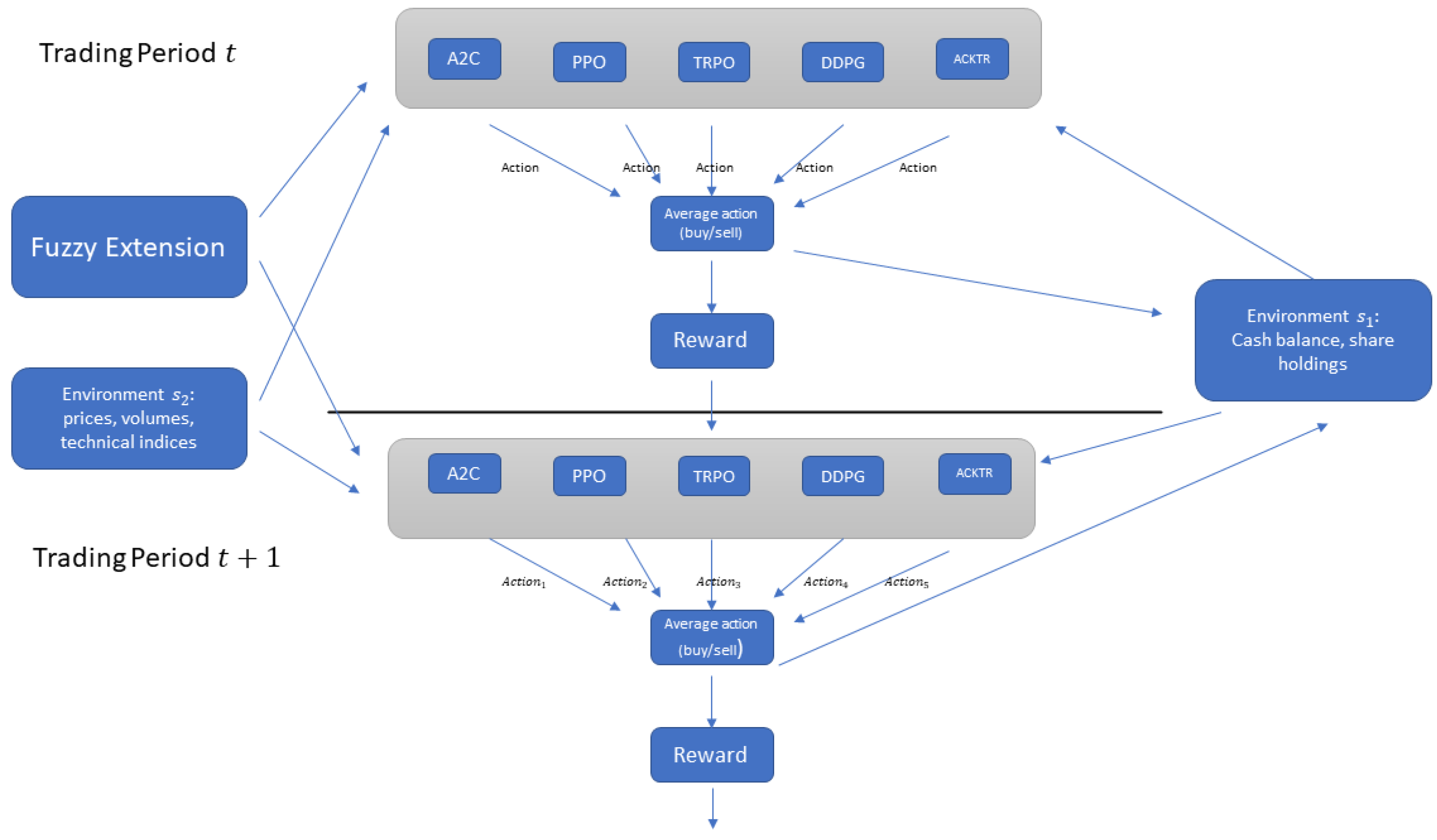
- Action a is a vector with a dimension equaling the number of stocks, M, whose positive components indicate buying and negative components indicate selling of the corresponding stocks. Each component of action a is a number between and 1, indicating the number of shares we buy or sell. For example, a number would mean that we sell shares of a stock, where H is a hyperparameter defining the maximum amount of shares for any single transaction. There are usually two ways to claim the maximum: the first way is to choose the same number of shares for all stocks; for example, would mean a single transaction can, at most, buy or sell 1000 shares of any stock; the second way is to choose the same value for all stocks, for example, a single transaction can at most have a total value of 100,000 USD. In this case, the number of maximum shares for each stock is different and is computed by 100,000 divided by the current stock price. In this work, we used the second way. is the stochastic policy that gives the probability of action a when facing state s. We denote as the action taken in period t. In our problem, for example, say for stock A, the action could be (1) buying shares of the stock and resulting in shares, or (2) holding, which results in , or (3) selling stocks and yielding . The action will also update the cash balance and other stocks and, therefore, reach the state . This action results in a reward, denoted by , which is the change in the portfolio’s total value.
- We also make the following assumptions and constraints. There will be no short selling. All selling transactions in the action vector are conducted before buying, and all buying transactions’ total value does not exceed the current cash amount plus the total value of all sell transactions. That is, the traders could use the cash received from selling stocks in a period to buy other stocks in the same period, but they could not borrow other cash. In addition, every single transaction’s total value does not exceed of the total portfolio value, where K is a hyperparameter.
- Value function and Q function are defined to be the value function of state s and the value function of state-action pair by following policy . In stock trading, means the expected future gain when facing state s, and means the expected return when facing state s and taking action a if the trader follows policy .
- Advantage function, denoted by , can be thought of as how much better state s would be if we take action a opposed to average. In many algorithms, subtracting the value function is called a baseline. In our approach, value function, Q function, and advantage function are predefined and embedded in the programming packages and need no extra attention.
2.2. Reinforcement Learning Algorithms
- (1)
- Advantage Actor-Critic (A2C)
- (2)
- Trust Region Policy Optimization (TRPO)
- (3)
- Proximal Policy Optimization (PPO)
- (4)
- Actor-Critic Using Kronecker Factored Trust Region (ACKTR)
- (5)
- Deep Deterministic Policy Gradient (DDPG)
2.3. Fuzzy Extension
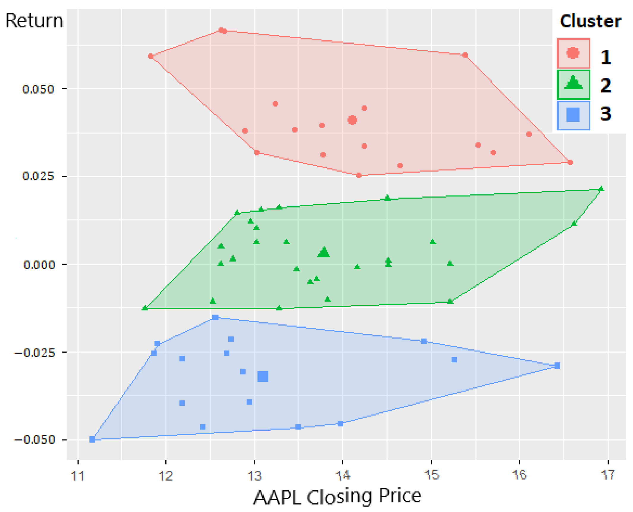
- choose moving window length , and using k-mean clustering on the rates of return to get groups with means and standard deviations, and , , respectively.
- For period , compute fuzzy degree , via the Gaussian membership function (Krasnyuk et al. 2022; Lin et al. 2006) as
- These fuzzy degrees, , are added as fuzzy extensions to obtain the final state space, which was stated in Section 3.
- repeat this process for all stocks and for all periods.
2.4. Ensemble
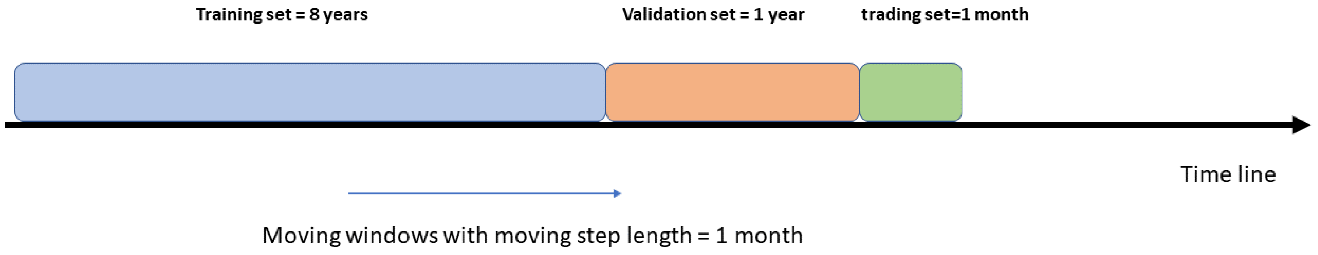
3. Datasets and Preprocessing
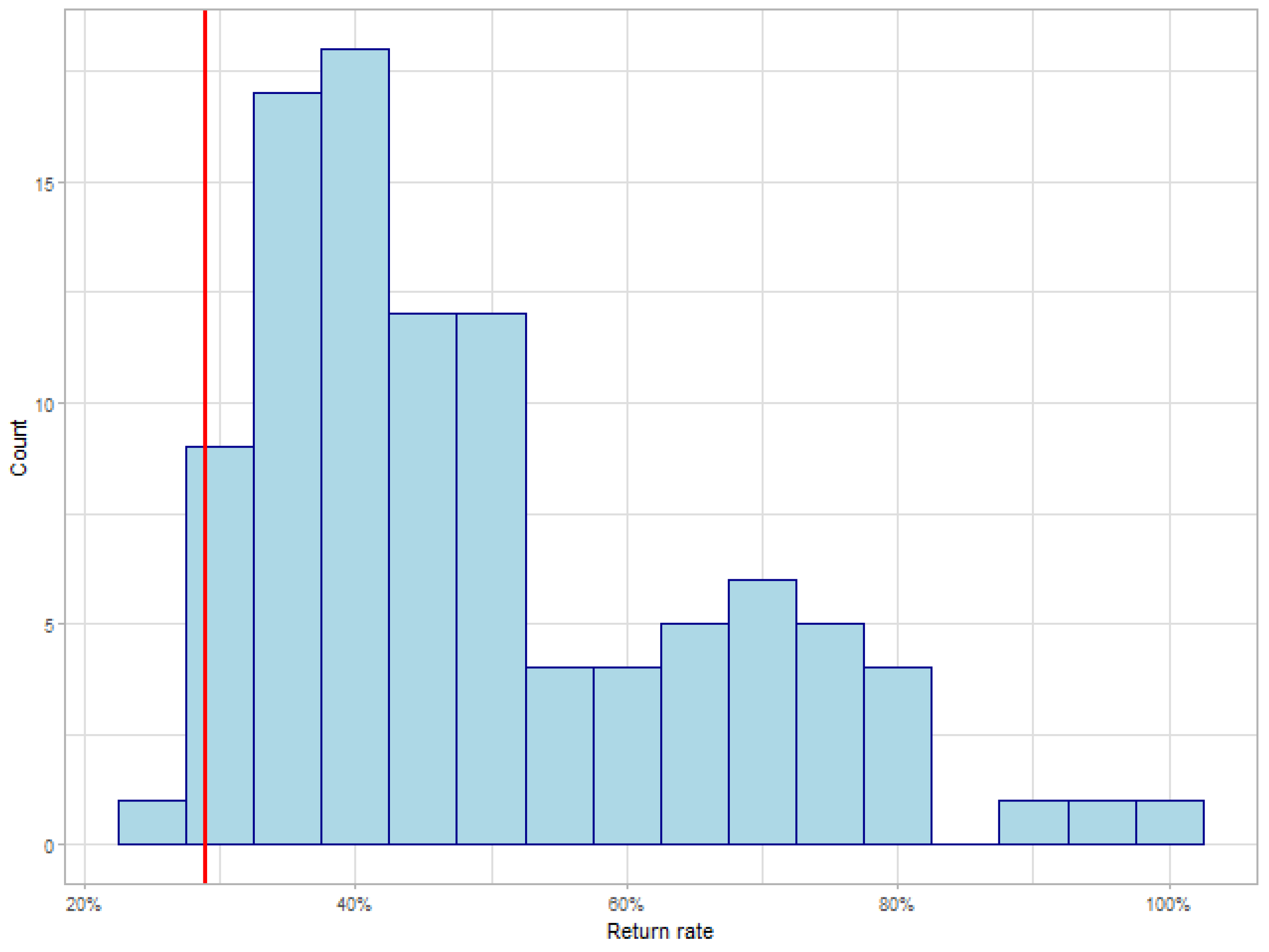
4. Results
5. Discussion and Conclusions
Author Contributions
Funding
Data Availability Statement
Conflicts of Interest
Abbreviations
| DL | Deep Learning |
| RL | Reinforcement Learning |
| LSTM | Long short-term memory |
| RRL | Recurrent Reinforcement Learning |
| CNN | Convolutional Neural Network |
| MACD | Moving Average Convergence/Divergence |
| A2C | Advantage Actor-Critic |
| TRPO | Trust Region Policy Optimization |
| PPO | Proximal Policy Optimization |
| ACKTR | Actor-Critic Using Kronecker Factored Trust Region |
| K-FAC | Kronecker-factored approximated curvature |
| DDPG | Deep Deterministic Policy Gradient |
| WR | Williams Overbought/Oversold Index |
| RSI | Relative Strength Index |
| CCI | Commodity Channel Index |
| ADX | Average Directional Index |
References
- Achiam, Joshua, David Held, Aviv Tamar, and Pieter Abbeel. 2017. Constrained Policy Optimization. Proceedings of the 34th International Conference on Machine Learning PMLR 70: 22–31. [Google Scholar]
- Balaji, A. Jayanth, D. S. Harish Ram, and Binoy B. Nair. 2018. Applicability of deep learning models for stock price forecasting an empirical study on bankex data. Procedia Computer Science 143: 947–53. [Google Scholar] [CrossRef]
- Chen, Peng, Dongyun Yi, and Chengli Zhao. 2020. Trading strategy for market situation estimation based on hidden markov model. Mathematics 8: 1126. [Google Scholar] [CrossRef]
- Chong, Eunsuk, Chulwoo Han, and Frank C. Park. 2017. Deep learning networks for stock market analysis and prediction: Methodology, data representations, and case studies. Expert Systems with Applications 83: 187–205. [Google Scholar] [CrossRef] [Green Version]
- Creamer, Germán, and Yoav Freund. 2010. Automated trading with boosting and expert weighting. Quantitative Finance 10: 401–20. [Google Scholar] [CrossRef]
- Dai, Min, Hefei Wang, and Zhou Yang. 2012. Leverage management in a bull–bear switching market. Journal of Economic Dynamics and Control 36: 1585–99. [Google Scholar] [CrossRef]
- Davis, Jonathan, and Alasdair Nairn. 2012. Templeton’s Way with Money. New York: Wiley Online Library. [Google Scholar]
- Deng, Yue, Feng Bao, Youyong Kong, Zhiquan Ren, and Qionghai Dai. 2016. Deep direct reinforcement learning for financial signal representation and trading. IEEE Transactions on Neural Networks and Learning Systems 28: 653–64. [Google Scholar] [CrossRef]
- Di, Xinjie. 2014. Stock Trend Prediction with Technical Indicators Using SVM. Independent Work Report. Standford: Leland Stanford Junior University, USA. [Google Scholar]
- Dunn, Olive Jean. 1961. Multiple comparisons among means. Journal of the American Statistical Association 56: 52–64. [Google Scholar] [CrossRef]
- Em, Olga, Georgi Georgiev, Sergey Radukanov, and Mariana Petrova. 2022. Assessing the market risk on the government debt of kazakhstan and bulgaria in conditions of turbulence. Risks 10: 93. [Google Scholar] [CrossRef]
- Fischer, Thomas, and Christopher Krauss. 2018. Deep learning with long short-term memory networks for financial market predictions. European Journal of Operational Research 270: 654–69. [Google Scholar] [CrossRef] [Green Version]
- Fu, Xingyu, Jinhong Du, Yifeng Guo, Mingwen Liu, Tao Dong, and Xiuwen Duan. 2018. A machine learning framework for stock selection. arXiv arXiv:1806.01743. [Google Scholar]
- Gold, Carl. 2003. FX trading via recurrent reinforcement learning. Paper presented at 2003 IEEE International Conference on Computational Intelligence for Financial Engineering, Hong Kong, China, March 20–23; pp. 363–70. [Google Scholar]
- Iliev, Nikola, Marin Marinov, Valentin Milinov, and Mariana Petrova. 2023. Is investment portfolio construction sustainable in the circular economy paradigm—The case of esg investment? In Circular Business Management in Sustainability. ISCMEE 2022. Lecture Notes in Management and Industrial Engineering. Cham: Springer, pp. 15–42. [Google Scholar]
- Jiang, Zhengyao, and Jinjun Liang. 2017. Cryptocurrency portfolio management with deep reinforcement learning. Paper presented at 2017 Intelligent Systems Conference (IntelliSys), London, UK, September 7–8; Piscataway: IEEE, pp. 905–13. [Google Scholar]
- Kakade, Sham, and John Langford. 2002. Approximately optimal approximate reinforcement learning. Paper presented at the Nineteenth International Conference on Machine Learning, San Francisco, CA, USA, July 8–12; pp. 267–74. [Google Scholar]
- Kloek, Teun, and Herman K. Van Dijk. 1978. Bayesian estimates of equation system parameters: An application of integration by monte carlo. Econometrica: Journal of the Econometric Society 46: 1–19. [Google Scholar] [CrossRef] [Green Version]
- Krasnyuk, Maxim, Iryna Hrashchenko, Svitlana Goncharenko, and Svitlana Krasniuk. 2022. Hybrid application of decision trees, fuzzy logic and production rules for supporting investment decision making (on the example of an oil and gas producing company). Access Journal 3: 278–91. [Google Scholar] [CrossRef] [PubMed]
- Lee, Sang, II, and Seong Joon Yoo. 2020. Threshold-based portfolio: The role of the threshold and its applications. The Journal of Supercomputing 76: 8040–57. [Google Scholar] [CrossRef] [Green Version]
- Leung, Mark T., Hazem Daouk, and An-Sing Chen. 2000. Forecasting stock indices: A comparison of classification and level estimation models. International Journal of Forecasting 16: 173–90. [Google Scholar] [CrossRef]
- Li, Bin, and Steven C. H. Hoi. 2014. Online portfolio selection: A survey. ACM Computing Surveys (CSUR) 46: 1–36. [Google Scholar] [CrossRef]
- Liang, Zhipeng, Hao Chen, Junhao Zhu, Kangkang Jiang, and Yanran Li. 2018. Adversarial deep reinforcement learning in portfolio management. arXiv arXiv:1808.09940. [Google Scholar]
- Lillicrap, Timothy P., Jonathan J. Hunt, Alexander Pritzel, Nicolas Heess, Tom Erez, Yuval Tassa, David Silver, and Daan Wierstra. 2015. Continuous control with deep reinforcement learning. arXiv arXiv:1509.02971. [Google Scholar]
- Lin, Chin-Teng, Chang-Mao Yeh, Sheng-Fu Liang, Jen-Feng Chung, and Nimit Kumar. 2006. Support-vector-based fuzzy neural network for pattern classification. IEEE Transactions on Fuzzy Systems 14: 31–41. [Google Scholar]
- Martens, James, and Roger Grosse. 2015. Optimizing neural networks with kronecker-factored approximate curvature. Paper presented at 32nd International Conference on Machine Learning, Lille, France, July 6–11; New York: PMLR, pp. 2408–17. [Google Scholar]
- Mnih, Volodymyr, Adria Puigdomenech Badia, Mehdi Mirza, Alex Graves, Timothy Lillicrap, Tim Harley, David Silver, and Koray Kavukcuoglu. 2016. Asynchronous methods for deep reinforcement learning. Paper presented at 33rd International Conference on Machine Learning, New York, NY, USA, June 19–24; New York: PMLR, pp. 1928–37. [Google Scholar]
- Moody, John, and Lizhong Wu. 1997. Optimization of trading systems and portfolios. Paper presented at IEEE/IAFE 1997 Computational Intelligence for Financial Engineering (CIFEr), New York, NY, USA, March 24–25; Piscataway: IEEE, pp. 300–7. [Google Scholar]
- Moody, John, and Matthew Saffell. 1998. Reinforcement learning for trading. Advances in Neural Information Processing Systems, 917–23. [Google Scholar]
- Moody, John, Lizhong Wu, Yuansong Liao, and Matthew Saffell. 1998. Performance functions and reinforcement learning for trading systems and portfolios. Journal of Forecasting 17: 441–70. [Google Scholar] [CrossRef]
- Murphy, John J. 1999. Technical Analysis of the Financial Markets: A Comprehensive Guide to Trading Methods and Applications. Penguin: New York: New York Institute of Finance. [Google Scholar]
- Nikolaev, Daniel, and Mariana Petrova. 2021. Application of simple convolutional neural networks in equity price estimation. Paper presented at 2021 IEEE 8th International Conference on Problems of Infocommunications, Science and Technology (PIC S&T), Kharkiv, Ukraine, October 5–7; Piscataway: IEEE, pp. 147–50. [Google Scholar]
- Oelschläger, Lennart, and Timo Adam. 2021. Detecting bearish and bullish markets in financial time series using hierarchical hidden markov models. arXiv arXiv:2007.14874. [Google Scholar]
- Ozbayoglu, Ahmet Murat, Mehmet Ugur Gudelek, and Omer Berat Sezer. 2020. Deep learning for financial applications: A survey. Applied Soft Computing 93: 106384. [Google Scholar] [CrossRef]
- Pal, Nikhil R., and James C. Bezdek. 1994. Measuring fuzzy uncertainty. IEEE Transactions on Fuzzy Systems 2: 107–18. [Google Scholar] [CrossRef] [PubMed]
- Rubinstein, Mark. 2002. Markowitz’s “portfolio selection”: A fifty-year retrospective. The Journal of Finance 57: 1041–45. [Google Scholar] [CrossRef] [Green Version]
- Schulman, John, Filip Wolski, Prafulla Dhariwal, Alec Radford, and Oleg Klimov. 2017. Proximal policy optimization algorithms. arXiv arXiv:1707.06347. [Google Scholar]
- Schulman, John, Sergey Levine, Pieter Abbeel, Michael Jordan, and Philipp Moritz. 2015. Trust region policy optimization. Paper presented at 32nd International Conference on Machine Learning, Lille, France, July 6–11; New York: PMLR, pp. 1889–97. [Google Scholar]
- Sezer, Omer Berat, Murat Ozbayoglu, and Erdogan Dogdu. 2017. A deep neural-network based stock trading system based on evolutionary optimized technical analysis parameters. Procedia Computer Science 114: 473–80. [Google Scholar] [CrossRef]
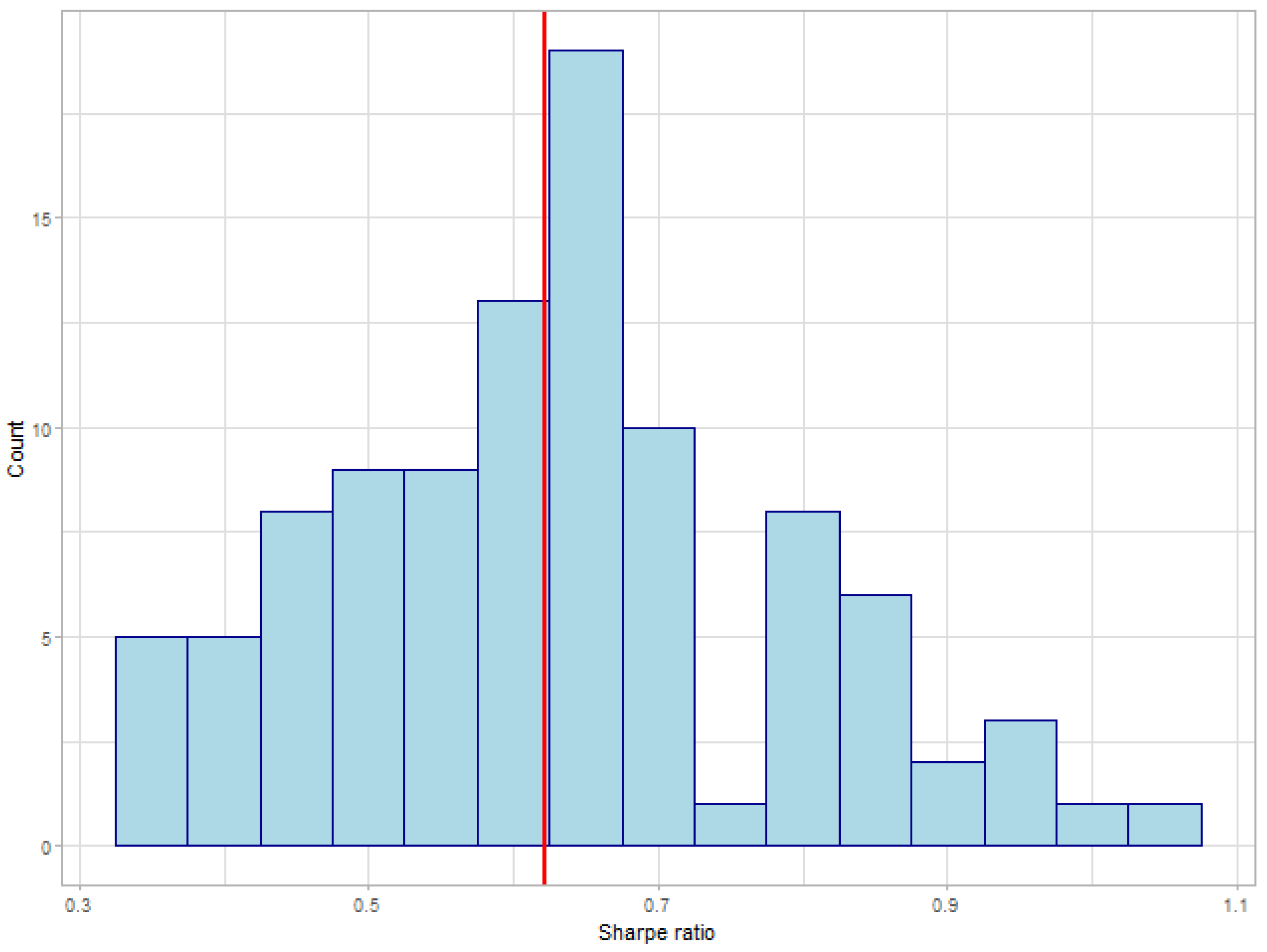
- Sharpe, William F. 1998. The sharpe ratio. Streetwise–the Best of the Journal of Portfolio Management 3: 169–85. [Google Scholar] [CrossRef] [Green Version]
- Silver, David, Aja Huang, Chris J Maddison, Arthur Guez, Laurent Sifre, George Van Den Driessche, Julian Schrittwieser, Ioannis Antonoglou, Veda Panneershelvam, Marc Lanctot, and et al. 2016. Mastering the game of go with deep neural networks and tree search. Nature 529: 484–89. [Google Scholar] [CrossRef]
- Singh, Sanjay Kumar, Shivendra Sanjay Singh, and Vijay Lakshmi Singh. 2023. Predicting adoption of next generation digital technology utilizing the adoption-diffusion model fit: The case of mobile payments interface in an emerging economy. Access Journal 4: 130–48. [Google Scholar] [CrossRef]
- Sutton, Richard S., and Andrew G. Barto. 2018. Reinforcement Learning: An Introduction. Cambridge: MIT Press. [Google Scholar]
- Van Dijk, Herman K., and Teunis Kloek. 1983. Experiments with Some Alternatives for Simple Importance Sampling in Monte Carlo Integration. Technical report. Amsterdam: Elsevier. [Google Scholar]
- Vargas, Manuel R., Carlos E. M. Dos Anjos, Gustavo L. G. Bichara, and Alexandre G. Evsukoff. 2018. Deep leaming for stock market prediction using technical indicators and financial news articles. Paper presented at 2018 International Joint Conference on Neural Networks (IJCNN), Rio de Janeiro, Brazil, July 8–13; Piscataway: IEEE, pp. 1–8. [Google Scholar]
- Vinyals, Oriol, Timo Ewalds, Sergey Bartunov, Petko Georgiev, Alexander Sasha Vezhnevets, Michelle Yeo, Alireza Makhzani, Heinrich Küttler, John Agapiou, Julian Schrittwieser, and et al. 2017. A new challenge for reinforcement learning. arXiv arXiv:1708.04782. [Google Scholar]
- Wu, Dingming, Xiaolong Wang, Jingyong Su, Buzhou Tang, and Shaocong Wu. 2020. A labeling method for financial time series prediction based on trends. Entropy 22: 1162. [Google Scholar] [CrossRef] [PubMed]
- Wu, Yuhuai, Elman Mansimov, Roger B. Grosse, Shun Liao, and Jimmy Ba. 2017. Scalable trust-region method for deep reinforcement learning using kronecker-factored approximation. In Advances in Neural Information Processing Systems. Cambridge: MIT Press, pp. 5279–88. [Google Scholar]
- Yang, Hongyang, Xiao-Yang Liu, Shan Zhong, and Anwar Walid. 2020. Deep reinforcement learning for automated stock trading: An ensemble strategy. Paper presented at the first ACM International Conference on AI in Finance, New York, NY, USA, October 15–16; pp. 1–8. [Google Scholar]
- Zhang, Zihao, Stefan Zohren, and Stephen Roberts. 2020. Deep reinforcement learning for trading. The Journal of Financial Data Science 2: 25–40. [Google Scholar] [CrossRef]


| Cluster Mean | Cluster SD | Fuzzy Extension Value | |
|---|---|---|---|
| increasing | 0.0411 | 0.0133 | |
| oscillation | 0.0029 | 0.01 | |
| decreasing | −0.0323 | 0.0108 |
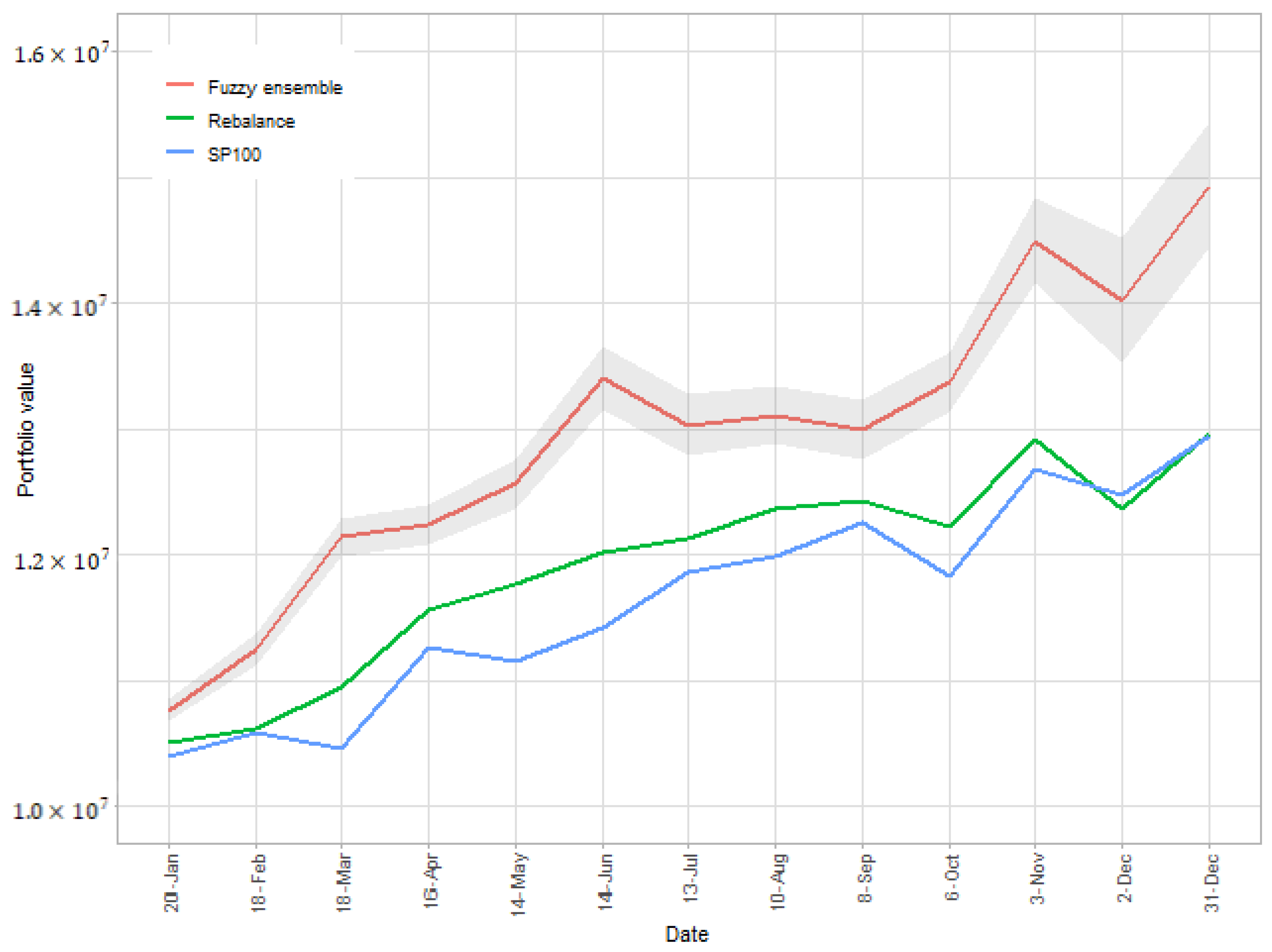
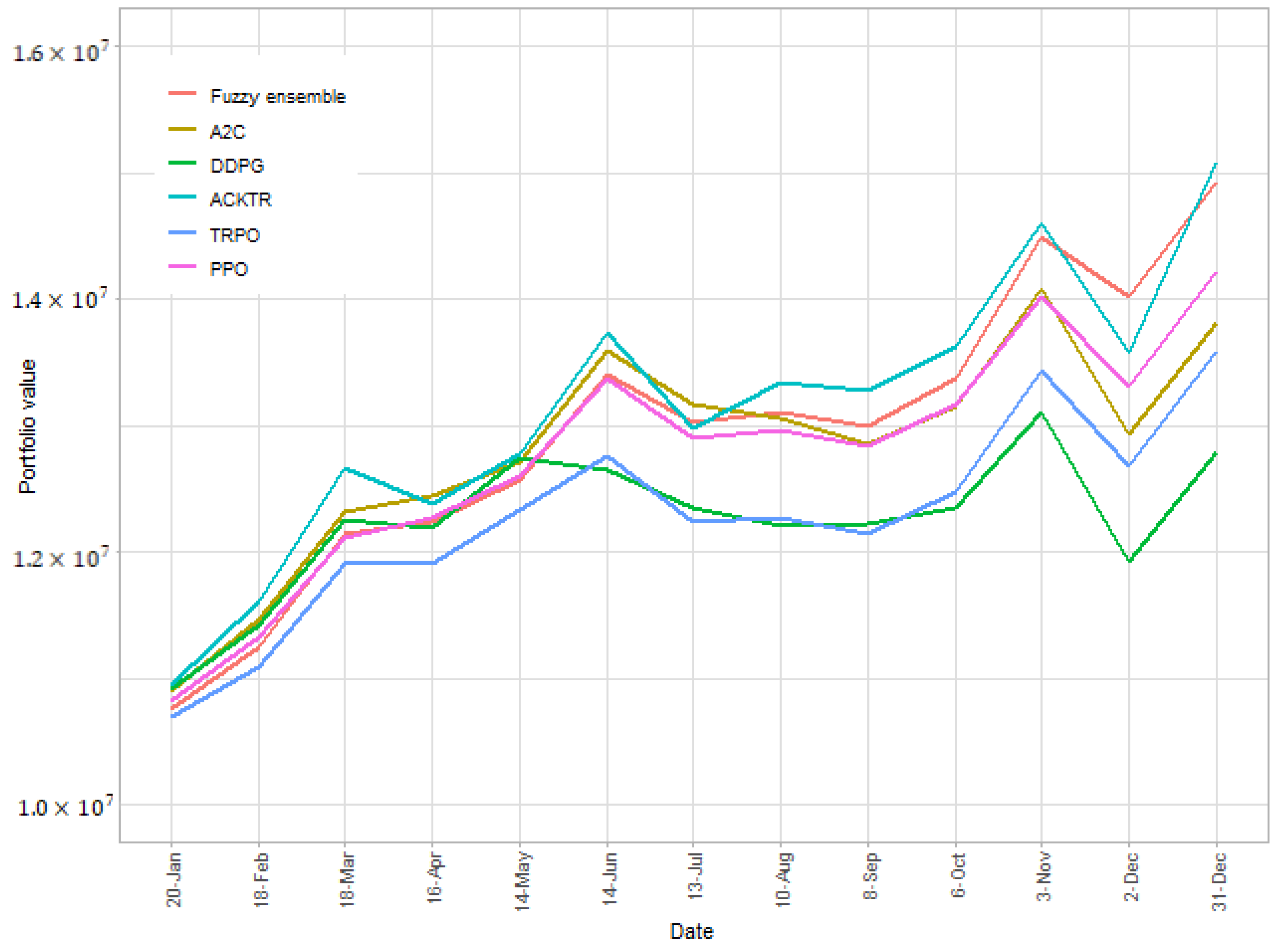
| Ours | SP100 | Rebalance | A2C | ACKTR | DDPG | TRPO | PPO | |
|---|---|---|---|---|---|---|---|---|
| Return Rate | 49.4% | 29.4% | 29.9% | 38.2% | 44.8% | 27.9% | 35.9% | 42.3% |
| Sharpe Ratio | 0.627 | 0.622 | 0.679 | 0.452 | 0.565 | 0.347 | 0.478 | 0.563 |
Disclaimer/Publisher’s Note: The statements, opinions and data contained in all publications are solely those of the individual author(s) and contributor(s) and not of MDPI and/or the editor(s). MDPI and/or the editor(s) disclaim responsibility for any injury to people or property resulting from any ideas, methods, instructions or products referred to in the content. |
© 2023 by the authors. Licensee MDPI, Basel, Switzerland. This article is an open access article distributed under the terms and conditions of the Creative Commons Attribution (CC BY) license (https://creativecommons.org/licenses/by/4.0/).
Share and Cite
Hao, Z.; Zhang, H.; Zhang, Y. Stock Portfolio Management by Using Fuzzy Ensemble Deep Reinforcement Learning Algorithm. J. Risk Financial Manag. 2023, 16, 201. https://doi.org/10.3390/jrfm16030201
Hao Z, Zhang H, Zhang Y. Stock Portfolio Management by Using Fuzzy Ensemble Deep Reinforcement Learning Algorithm. Journal of Risk and Financial Management. 2023; 16(3):201. https://doi.org/10.3390/jrfm16030201
Chicago/Turabian StyleHao, Zheng, Haowei Zhang, and Yipu Zhang. 2023. "Stock Portfolio Management by Using Fuzzy Ensemble Deep Reinforcement Learning Algorithm" Journal of Risk and Financial Management 16, no. 3: 201. https://doi.org/10.3390/jrfm16030201