Article

The Impact of M&As on Shareholders’ Wealth: Evidence from Greece

by
George Giannopoulos
1,
Alexandra Lianou
1 and
Mahmoud Elmarzouky
2,*
1
Kingston Business School, Kingston University, Kingston Hill, Kingston Upon Thames, London KT2 7LB, UK
2
Aston Business School, Aston University, 295 Aston Express Way, Birmingham B4 7UP, UK
*
Author to whom correspondence should be addressed.
J. Risk Financial Manag. 2023, 16(3), 199; https://doi.org/10.3390/jrfm16030199
Submission received: 3 February 2023 / Revised: 3 March 2023 / Accepted: 4 March 2023 / Published: 14 March 2023
(This article belongs to the Special Issue Contemporary Issues on Auditing and Financial Reporting)

Abstract

:
This study aims to investigate the effect of mergers and acquisitions (M&A) on shareholders’ wealth. Additionally, this study investigates the impact of the economic crisis during 2007–2008 on the shareholders’ perceptions of gaining additional value from mergers and acquisitions. In this paper, a sample of 84 M&As from 2006 to 2015 in Greece are studied to investigate the effect on shareholders of bidder companies. We find significantly negative abnormal returns just before the announcement of M&A, which negatively affects the bidder firms’ value. It is also observed that after 2009 M&A cases decreased, maybe because of the crisis in Greece that changed the investors’ perception of a value-destroying event. Companies that engage in M&A activities during economic downturns tend to experience a decline in shareholder value. This could be due to various factors, such as increased uncertainty and risk associated with such activities during economic uncertainty. By understanding the potential impact of such activities on shareholder value, companies can make more informed decisions about whether and when to pursue M&A opportunities.

1. Introduction

In today’s business world, prediction or speculation, and intuition have a significant impact on the market value and future growth of any organization. A manager must be able to predict a firm’s future activity and cash flow to raise and hold its market value. Predictions made with proper methodology allow potential investors to be motivated to invest their funds in a company. Theoretically, mergers and acquisitions are believed to be a process of achieving synergy and are presumed to gain extra strength in the financial capabilities, market size, or knowledge base of the new company. Therefore, information on M&A is expected to be treated as “good news” for the investors, employees of both firms, and even existing or potential customers. Thus, investors would gain extra value for their shares and eventually might earn some extra money, hence premium, by selling their stocks at the time of announcing the “good news”, i.e., predicting and discounting a future increase in share price. However, empirical evidence does not indicate the same scenario every time. Some studies suggest that the motivation behind an M&A and the unequal distribution of benefits among the bidder and target firms are two main reasons creating conflict and thus hindering the natural process of adding up more value to the new company.
The primary objective of this study is to present additional empirical evidence of M&A in Greece that resulted in abnormal returns and to examine the impact of the economic crisis on the abnormal returns of acquiring firms from M&A. This study also applies relevant theories to explain the reasons why some M&As are successful in generating abnormal returns while others are not.
This paper aims to answer the following research questions:
Are there statistically significant abnormal returns of Greek bidding firms around M&A announcements? Do different definitions of event windows affect the conclusions about M&As’ effects on value creation? Are some statistical properties, like non-normal distribution, responsible for differences in findings? Did the economic crisis in Greece change the effect of M&As on bidders’ value creation?
We contribute to the current literature in several ways. First, to the best of our knowledge, this is one of the first papers that investigated the impact of the economic crisis during 2007–2008 on the value-creation process of mergers and acquisitions in Greece. It is also important to examine if there are changes in the perception of investors toward M&As in Greece, especially after the economic crisis. These observations will be immensely helpful for further research in this field if any positive evidence comes out through this study.
Mergers and acquisitions (M&As) have been a popular strategy for firms seeking to expand their operations, gain market share, and increase profitability. However, the impact of M&As on shareholders’ wealth has been a subject of intense debate. In Greece, several studies have investigated the effect of M&As on shareholders’ wealth, and the results have been mixed. Some studies suggest that M&As have a positive impact on shareholder wealth, while others find no significant effect or even negative effects. Overall, it seems that the impact of M&As on shareholders’ wealth in Greece depends on various factors, such as the characteristics of the acquiring and target firms, the financing structure of the deal, and the economic and regulatory environment. Despite the mixed findings, M&As remain a popular strategy in Greece, and firms are likely to continue pursuing such deals in the future.

2. Literature Review

A successful M&A is expected to result in a comparatively larger company with stronger resources and more accessible finance. It is also expected that the new company will have more cashflows than those of the merged companies. It would also find a decrease in competitive forces, cost efficiency, and other positive changes. On the other hand, because of more stable cash flows, the new company would enjoy lower borrowing costs as the creditors and lenders would feel more comfortable offering credit facilities.
However, not all M&As result in these positive consequences. According to Brealey et al. (2001), failing to fully integrate the merged companies may be the outcome of employees’ and managers’ fear of a change in their working status and/or conflicts between different attitudes (Monga 2021; Arasa 2020; Tampakoudis and Anagnostopoulou 2020). Fears that relate to a working status include loss of employment, salary decrease, movement into a lower administrative level/position of lower social status or geographic area, increased performance standards, increased control, need for additional training, etc. Attitude-related obstacles may result from past “wars” between the merged companies (e.g., two former competitors that were fighting each other now must join the same “army”), bad experiences with M&As in the past (e.g., people within the organization suffered a lot after past M&As), personal reasons (e.g., a different way of “doing things”), etc.
Except for behavioral reasons, an M&A may fail because of incomplete or insufficient evaluation of potential benefits, checks of the target company’s financial condition, and so on (see AT Kearney, Inc. 1999; and Weber and Camerer 2003). Uncontrolled factors may also contribute to such failures. Protopapas et al. (2003) note that markets are sometimes unpredictable to such an extent that may rip off any synergy regarding market share, decreased competition, etc. Furthermore, M&As may cause governmental action to protect working contracts, safeguard employment, and prevent from monopolies being formed, among others.
Heaton (2002) also notes that some M&As should not have taken place at the beginning because of questionable motives (this is not the case of innocent mistakes during the evaluation phase). The author explains that, in such cases, M&As are not the outcome of targeted synergies or any other related benefit but, rather, they stem from managers’ vanity, what one could call “managerial hubris”. When managers move into an M&A driven by their will to find themselves in an “empire building” (i.e., put themselves in charge of a larger organization) and, hence, become more prestigious, the potential of achieving true benefits is lessened. Furthermore, the more a company attempts to acquire or merge with another one, the higher the bid it must offer to accomplish the agreement. It is obvious that the bid cannot increase infinitely because, after a certain level, added value will no longer be possible to achieve.
The benefits of M&As may be investigated based on two performance criteria, i.e., the operating and other types of performance except for stock prices and the returns earned by the stockholders of bidders, targets, or both. The first criteria deal with M&As’ expected benefits in terms of the firm’s profitability, return on investment, and other measures of financial performance (Teti and Tului 2020). In this case, the newly formed firm is compared with other similar companies in the industry or the industry average.
The second criteria deal with M&As’ effects on the stock prices of bidders and/or targets. In most cases, the value creation for bidders becomes the main concern of related investors because the number of listed bidders is normally higher than that of targets, and therefore, stock data are more frequently available for bidders than for targets. However, in this criterion, the value creation is measured with cumulative abnormal returns or cumulative average abnormal returns.
Dodd and Ruback (1977) investigate the effect of M&As on abnormal returns in the US Using a period of 73 up to 14 months before the event and 14 up to 73 months after the event, they find that during the month of the M&A announcement, the stockholders of target firms earn abnormal returns of approximately 21% if the transaction is accomplished and approximately 19% in case the M&A is not completed. By contrast, stockholders of bidder firms earn significantly lower abnormal returns of approximately 3%.
Dodd (1980) studies the abnormal returns of merged companies in the US during 1970–1977 one day before and on the day of the event. He finds that the cumulative abnormal returns of bidders are significantly negative and equal to −1.09% during the event window while being equal to +0.8% during the 20 day period before “day −1”. By contrast, stockholders of target firms enjoy CARs of +13.41% and 21.78%, respectively, for the two time periods reported above. Asquith (1983) estimates CARs for a 2 day event window in the US during 1962–1976. The study reveals that CARs near the M&A equal 0.2% and are not significantly different from those computed for the 20 day period before “day −1” for bidders. By contrast, CARs are +6.2% for target firms in the event window and +13.3% for the 20 day period before “day −1”.
Eckbo (1983) performs a similar study for the period 1963–1978 but uses a 3 day event window (days are −1, 0, and +1). The author finds that stockholders of bidders suffer negative CARs of 0.07% compared to the positive ones (+1.58%) they enjoy during the 20 day period before the event. CARs for target firms are +6.24% and +14.08% for the two periods, respectively.
Using a sample of bidder firms during 1969–1974, Malatesta (1983) computes CARs for the 30 days until the event and reports CARs of 0.9% for bidders and +16.8% for targets.
Franks and Harris (1989) investigated the effect of M&As in the UK and the US during 1955–1985. The authors use a 3-day event window (−1, 0, and +1) and a 2-month estimation period until day −11 (day −71 until −11). The study reveals that UK target firms suffered significant negative CARs of 3.6% while their US counterparts enjoyed insignificant positive CARs of 0.1%.
Agrawal et al. (1992) computed CARs for merged companies in the US during 1955–1987 and found that 5 years after the M&A, only 44% approximately of merged companies enjoyed positive CARs, which averaged −10.26%. Sudarsanam et al. (1996) investigated the effect of M&As on synergies and stock performance in the UK during 1980–1990 using the market model. Expected returns are computed for the period of 290 to 41 days before the M&A announcement. The study’s findings suggest that M&As create value for the stockholders of both the bidders and the targets. However, when highly valued companies merge with companies of lower value, the stockholders of the former suffer losses in terms of value.
Higson and Elliott (1998) investigated the effect of M&As in the UK from 1975 to 1990 and found that bidders suffered negative CARs during the announcement period, but CARs are zero for the 3 year period after the event. Goergen and Renneboog (2004) study the effect of M&As that took place in Europe during the 1980s. CARs are computed for a time window of 120 days equally split before and after the event. The study’s findings suggest that stockholders of target firms enjoy CARs of 9% that reach 23% if the 2 month period before the event is also accounted for. Stockholders of bidders also enjoy positive CARs but to a much lesser degree (0.7%).
Martynova and Renneboog (2006) study M&As in Europe during 1993–2001 and find CARs of +0.95% for target firms for a 40 day period before the event.
Antoniou et al. (2006), define a 3 day event window for M&As in the UK during 1985–2004. According to their results, CARs are −1.3% for the event window [−1,1] and −1.4% if the event window changes to [−2,2]. Petmezas (2009) defines a 5 day time window (−2 to +2 days) and report positive abnormal returns for UK bidders during 1984–2003.
Rani et al. (2013) investigate the effect of corporate governance on M&As’ CARs in India during 2003–2008 and use multiple event windows, namely 3, 5, 7, and 11 days around the event. The authors report that CARs for bidders were 0.99% 1.54% 1.96%, and 1.95%, respectively, for the above-mentioned event windows.
Varmaz and Laibner (2016) investigate M&As in the US during 1999–2015 and compute CARs for 13 periods ranging from the day of announcement until 40 days around it. According to their findings, bidders enjoy positive CARs for periods up to 5 days before and 5 days after M&As but they suffer negative CARs in longer periods around the event (Wasilewski et al. 2021; Tampakoudis et al. 2022). By contrast, CARs are positive for targets no matter what time period around the event is considered.

3. Research Design

3.1. Data Sampling

Information on M&As in Greece comes from the annual reports of the Hellenic Capital Market Commission (HCMC). Among others, these reports present the title and date of M&As that took place during the respective year. We use this date as the date of the event. Unfortunately, in some cases, no date is reported (only the calendar year during which the M&A took place is available) and, hence, the corresponding M&As are excluded from the sample. The available reports come from the period 2006–2015 and produce a sample of 179 M&As during that period. However, there were 7 M&As that took place in 2005 and were reported in the 2006 report. Moreover, the number of M&As without any specific date is 13. Consequently, the search for stock data regards 159 cases (as, from the original sample of 179 M&As, we excluded the aforementioned 20 M&As). It must be emphasized that the term “case” here does not imply “firms” but M&As because some firms participate in M&As more than once during the reviewed period. Therefore, the number of firms is less than 159. The distribution of these 159 M&As during 2006–2015 is presented in the following Figure 1 (number of M&As per year).
As can be seen in Figure 1, the effect of the recent crisis is more than evident in M&A action in Greece. Although the annual number of M&As is about 20–25 until 2008 (the year the crisis began in the US), we note an extensive decrease afterward that leads to an annual number of M&As around 10–13 except for 2011. It must be noted that the higher number of M&As during 2011 is due to M&As by banks (probably because of recapitalization procedures) and fish farms (an industry that had long struggled to survive). An χ2 test of goodness-of-fit led to a value of 2.8, which is significantly lower than the critical value of χ2 for k − 1 = 10 − 1 = 9 degrees of freedom (3.325) at the 5% level. This means that the assumption of uniform distribution of M&A numbers across the sampled year is rejected at the 5% level. The 159 M&As are distributed across listed and non-listed firms as follows. There are 157 listed and 2 non-listed bidders. There is no relevant information available for 13 targets and the rest 146 of them are divided into 24 listed and 122 non-listed ones.
Stock data were searched for in two databases. We begin our search at Yahoo Finance and in cases where no available data existed, we moved on with searching it at the website of “Naftemporiki”, one of the oldest Greek portals dealing with economic information and information regarding the Hellenic Exchange (Athens Stock Exchange). Since our maximum estimation window starts 160 days before the event (see next section) some data come from 20.05 (for M&As that took place in 2006). This procedure led to the following. First, none of the two databases reported data available for 65 bidders either because the company is now delisted or because it has merged with another one in the past and its stock stopped trading. For 9 firms, no suitable data were found, i.e., although the company is included in the database, the stock data provided are outside the estimation period. One case had also to be excluded because the M&A was announced during the period of capital controls (imposed on 28 June 2015) that left the stock exchange out of work until mid-August for some weeks (there are no data for the event window). Consequently, a sample of 84 M&As with data available for listed bidders was formed. Recalling that the sampling procedure started with 179 M&As, this figure gives us approximately 47% of cases with available data. The following Figure 2 summarizes the sample’s “identity”.
As expected, delisted companies are much more pronounced in the sub-sample that covers the period until 2009. Focusing solely on cases with available data (totalling 84), those with data until (after) 2009 form 34% (66%) of all cases. Although the sample size seems to be small, it is comparable to other studies that concern much larger economies compared to the Greek one. For instance, Goergen and Renneboog (2004) examine a sample of 228 observations for the European market, while the sample size used by Chang (2002) for the US market consists of 281 cases.

3.2. Selection of Statistical Model

This study follows one of the most widely used methods to investigate M&As’ abnormal returns, namely the event study approach. The main purpose of this methodology is to isolate excess stock returns because of the “event” under investigation, in our case the M&A. This methodology was initially developed by Fama et al. (1969) followed by Brown and Warner (1980, 1985). In brief, the event study methodology consists of comparing actual stock returns with expected ones around a time “window”, i.e., a period that starts before the event and ends after it, the difference is called “abnormal return”. The formula to compute abnormal returns is as follows:
ARj,t = Rj,t − E(Rj,t)
where
j = 1, 2, …, N is the index of companies (N is the number of sample firms)
t = 1, 2, …, T is the index of time periods (T is the number of T periods examined)
AR stands for “abnormal returns”
R stands for “actual returns”
E(R) stands for “expected returns”
In simple terms, the abnormal return is the excess return earned by stockholders because of the M&A and can be either positive or negative. Obviously, an M&A leading to positive (negative) abnormal returns creates (destroys) value. Returns can be computed as simple percentage change from one period to another, i.e., Rt = (Pt − Pt−1)/Pt−1 where P stands for the stock price. With respect to the unit of time, there is no absolute consensus. Some researchers support the view that daily returns should be used while others suggest using monthly returns to avoid extreme deviations from normality. The distribution of daily returns may deviate from normality because of instant “ups” and “downs” of stock prices while (average) monthly returns are generally considered a “safer” choice because the effect of stock price “ups” and “downs” on stock returns’ distribution is somewhat less severe. In this study, we use daily returns because, in our opinion, they better reflect what happens in reality regarding the way markets act. To explain, we find it rather unrealistic to assume that markets, i.e., the investors, are not (or do not think of being) involved in everyday transactions. Monthly returns imply, at least to a certain degree, that markets form their expectations every 30 calendar or 25 working days. Obviously, this cannot be the case although, from a methodological standing, it may help deal with technicalities like the deviation from normality. It must be noted, however, that the estimation periods applied here (see below) are too long for deviations from normality to be an issue.
The first step to performing an event study analysis is to define the time window reported earlier. Some studies apply a 60 day period, e.g., Franks and Harris (1989), divided evenly before and after the “event” while others apply wider time windows reaching up to 240 days around the event, e.g., Bradley et al. (1988). Normally, the day of the event (or its announcement) is set to be “day 0”. Thus, the days that precede the event are −1, −2, etc. where lower values imply greater distance from the event, e.g., “day −25” means 25 days before the event. In a similar way, days after the event take positive value but, in this case, lower values imply that the respective day is closer to the “event day”. It must be noted that some researchers favor the use of different time windows within the same study to capture the effect of time span on abnormal returns. This approach is also adopted here for this reason. In particular, we set two different event windows to check if this leads to significantly different findings. The “short” time window is set to 3 days, following Chakrabarti et al. (2005), i.e., [−1, 1], while the “long” one is set to 11 days following Rani et al. (2013), i.e., [−5, 5].
E(R) is estimated using several models (e.g., the Capital Asset Pricing Model or the Market Model) and past data for stock returns for the estimation period, which may vary from a few months to almost a year. Data availability and the ability to compare findings with similar studies are among the reasons for the different approaches among researchers. The estimation period stops earlier than the left limit of the event window (see above). For example, if the event takes place on 30 November 2016 and the researcher sets a 3 day event window, data to estimate E(R) will come from the period 30 October 2013 to 30 October 2016 assuming a 3 year estimation period. The 30 days between the end of the estimation period and the event window are set to avoid possible effects on stock prices (and returns) because of suspicions or rumors regarding the event. In this example, it is implied that there has been no such effect or, simply put, that investors (or “the market”) had no idea of the forthcoming M&A 30 days before it was announced. Following Chakrabarti et al. (2005), our estimation period is set to 119 days and stops 41 days before the event, therefore it is set as [−160, −41]. This leaves 40 working days between the end of the estimation period and the event or approximately 2 calendar months, which should be enough time for the market not to have discounted any benefit of the forthcoming M&A. Of course, this choice is subject to criticism.
Once the estimation period and event window have been defined, the abnormal returns are computed for each day in the event window. Then, we compute the average for each event day for all M&As included in the sample to get the average abnormal return (AAR) attributed to M&As. Summing all AARs provides the cumulative average abnormal return (CAAR) due to M&As that is, obviously, a measure of value creation, if positive, or value destruction, if negative, of M&As at the market under investigation. Following Varmaz and Laibner (2016), value creation is investigated with a t-test to check if abnormal returns on each day of the event window are (or are not) significantly different from 0 and/or check if the average cumulative abnormal returns (average CARs), i.e., the cumulative abnormal return earned on average from investors, are significantly different from 0. The difference between the two approaches lies in that the first one tests daily effects around the M&A announcement while the second examines the total effect for the period around the M&A announcement.
We use the Market Model and linear regression (Varmaz and Laibner 2016) to estimate expected returns as follows (where m stands for “market”):
E(Rit) = aˆi + βˆiRmt
The market is represented by the FTSE/XA Large Cap index that consists of the 25 largest, in terms of market capitalization, listed companies in Greece. This index was chosen because it includes most of the bidders examined here. Another reason is that other indexes, e.g., the General Index or the FTSE/XA Mid Cap, may be affected by zero returns concerning inactive stocks, temporarily delisted companies, companies under supervision, etc. Data for the market were downloaded from “capital.gr”, a Greek financial information website.
All statistical tests are performed at the 5% level of significance (unless otherwise stated). The notations used for the variables examined are given in Table 1.
With respect to the sampling procedure, it is noted that relevant data are hard to find especially when they are related to old M&As. This happens because some firms have been delisted or merged and, thus, their stock data are not available by widely used databases. Although this issue was not completely dealt with, the size of the sample used is comparable to that of samples regarding much larger markets. Nevertheless, there exists preliminary evidence suggesting that the recent crisis negatively affected the number of M&As in Greece. To check for possible effects of different methodological designs, two different event windows, in terms of duration, are considered to investigate abnormal returns around M&As.

4. Empirical Data Analysis and Discussion

4.1. Normal Distribution Tests

Table 2 reports the results of the Kolmogorov–Smirnov and Shapiro–Wilk tests for the normal distribution of ARs, AARs, and CARs.
Table 2 shows that the hypothesis of normal distribution is rejected for all variables irrespective of the test considered (sig < 0.05). To avoid the effect of extreme deviation from normality we performed an outlier check using boxplots to delete extreme outliers and then test again for normal distribution. For most variables, deleting a few outliers leads to boxplots without extreme outliers. Boxplots of initial and trimmed data are given in Appendix A. For each variable, the boxplot produced for initial data is contrasted with that after trimming extreme outliers.
Table 3 suggests that deviation from normal distribution has been reduced for all variables. This is evidenced by the increased p-values of corresponding tests. However, despite deleting extreme outliers, the assumption of a normal distribution is still rejected (sig. < 0.05) for most variables (11 out of 13). It is then useful to move on with reporting evidence regarding the initial dataset and the dataset with deleted extreme outliers to see whether findings change from one dataset to the other. In the remainder of the paper, the two samples will be called “initial” and “trimmed”, respectively.

4.2. Descriptive Statistics

Table 4 reports descriptive statistics, namely mean, median, standard deviation, kurtosis, and skewness, for all variables and both samples.
From Table 4, we see that non-normality affects descriptive statistics to a very extended degree. For instance, the mean of abnormal returns 5 days before the event (AR_MINUS_5) is −963.262 and 0.006 for the initial and trimmed sample, respectively. Another piece of evidence regarding the effect of non-normality relates to differences between the mean and median. For the variable reported above, the difference between the two metrics is −963,263 (= −963.262 − 0.001) and 0.003 (= 0.006 − 0.003) for the two samples, respectively. Additionally, the standard deviation computed in the initial sample is hundreds of thousands higher than that computed in the trimmed sample. For example, the standard deviation of abnormal returns four days before the event (AR_MINUS_4) in the initial sample is more than 345,060 than that in the trimmed one (= 11387.225/0.033). Finally, both the skewness and kurtosis suggest that, on the one hand, there are extreme deviations from normality in the initial sample and, on the other hand, dropping out extreme outliers leads to less severe non-normality. To explain, values of skewness in the initial sample are very far from 0 (which corresponds to normal distribution) while those of kurtosis are very far from 3 (which corresponds to normal distribution). By contrast, when the trimmed sample is used, skewness is close to 0 (the largest difference, in absolute value, relates to abnormal returns four days after the event, AR_PLUS_4) while the value of kurtosis is much closer to 3 when compared to the value of kurtosis in the initial sample (although still away from a value that would permit to assume a normal distribution). The improvement achieved by deleting outliers is also evident in the histograms presented in Appendix B. As in the case of boxplots, we contrast histograms prepared for the initial sample to those prepared for the trimmed sample. With minor exceptions, the distribution of all variables in the trimmed sample is, approximately, bell-shaped while that in the initial sample is far from even approaching being such. This is additional evidence of the usefulness to compare evidence (and thus, conclusions drawn) based on initial data and trimmed data.

4.3. Findings on Abnormal Returns

4.3.1. Daily Abnormal Returns

Table 5 reports the findings regarding daily abnormal returns, i.e., abnormal returns from 5 days before the event until 5 days after it. The hypothesis tested here is that ARs are not significantly different from 0. For reasons already explained, the respective analysis is performed for both the initial and the trimmed samples.
Once again, it becomes apparent that extreme deviations from normality may significantly affect empirical findings and, thus, the conclusions about value creation or destruction because of M&A. To explain, when the initial sample is considered, we find that abnormal returns are, on average, significantly different from zero only on the day of the event announcement, i.e., day “0” (t-sig < 0.05). However, this result may be a manifestation of the non-normal distribution of the abnormal returns in the initial sample. By contrast, if the trimmed sample is considered, we find mixed evidence of daily abnormal returns. In particular, the daily abnormal returns are, on average, not significantly different from zero 5 to 2 days before the event (t-sig > 0.05 for AR_MINUS_5, AR_MINUS_4, AR_MINUS_3, and AR_MINUS_2) and become significantly negative on the day that immediately precedes it. On the day of the event and the two days after it, abnormal returns are not significantly different from 0, however, they become significantly positive on the 3rd day after the event, negative on the 4th, and again positive on the 5th day after the event. It is then concluded that M&As lead to significant negative abnormal returns immediately before they are announced and possibly on the day of the announcement. With respect to the days after the event, we find mixed evidence. Additionally, it is evident that conclusions depend upon the sample studied and may substantially change if abnormal returns are far from being normally distributed, as in the initial sample.

4.3.2. Cumulative Abnormal Returns

Table 6 reports the findings regarding cumulative abnormal returns for the 2 event windows considered, i.e., [−1, 1] and [−5, 5]. Here, the hypothesis tested is that CAARs are not significantly different from 0 (at the 5% level) in both the initial and the trimmed samples.
The findings presented in Table 6 lead to conclusions that are identical to those reached from the analysis of the preceding table. Hence, it is shown that M&As lead to neither positive nor negative cumulative abnormal returns around the day they are announced no matter what event window is examined, 3 day or 11 day. As far as the effect of non-normality is concerned, the evidence suggests that the hypothesis of non-zero returns is more clearly rejected if data without extreme outliers are considered.

4.4. Discussion

The previous section made clear that, in general, M&As in Greece do not have the hypothesized value-creating effects for stockholders of bidder firms. However, there is some evidence suggesting the existence of non-zero abnormal returns but without a clear pattern. It makes no obvious sense that daily abnormal returns are significantly negative one day before the event, then turn into not being significantly different from zero until 2 days after the event, and follow an “upside-down” trajectory from the third to the fifth day after the event being significantly positive, negative, and then again positive. The only reasonable explanation that comes to mind for this “strange” behavior of returns is that bidders’ stockholders are somewhat surprised by the M&A announcement and engage in very active trading until they clarify if the M&A is value-creating or not. This perhaps could explain the “ups and downs” of abnormal returns a couple of days after the announcement.
Another possible explanation is related to the methodology used to test the assumption of zero abnormal returns. Given that normality is not achieved even when dropping out extreme outliers, it is possible for parametric tests, like the t-test used here, to be misleading. To check for this possibility, we also performed the Wilcoxon signed-rank test to test the hypothesis that the median value of abnormal returns (in every computational version) is equal to zero. These results are reported in Table 7 (medians are reported for convenience).
Based on what is reported in Table 7 for the initial sample, all significant abnormal returns are negative. With respect to daily ones, we note that stockholders of bidders suffer negative abnormal returns on days −4, −3, −1, 0, and 4. Furthermore, the median of cumulative average abnormal returns in the short window is also significantly less than zero, suggesting the existence of negative abnormal returns during the 3 day period around the event. By contrast, there is no evidence to suggest that average or cumulative abnormal returns are not zero in the long window, i.e., 11 days around the event. However, the effect of non-normality seems to be present also here given that the median test in the trimmed sample leads to almost totally different findings. To explain, significant and negative (daily) abnormal returns are found only on the day before the event (this is in line with results regarding the initial sample). By contrast, stockholders of bidders enjoy significant and positive (daily) abnormal returns 3 and 5 days after the event. Moreover, no evidence of significant abnormal returns is found for any of the event windows considered.
To check further, we compare the percentages of cases with positive abnormal returns in the initial sample (extreme values do not affect this kind of analysis because they are classified as any other positive or negative value). We use dummy variables (denoted with “_DUMMY” at end of the so far used ones) that take the value of 1 if the abnormal return is positive and 0 otherwise. The percentages of positive and negative abnormal returns along with goodness-of-fit χ2 test results, are reported in Table 8.
The results reported in Table 8 suggest that there are significant negative (daily) abnormal returns one day before the event. In particular, we see that 56 out of 84 M&As (67%) lead to negative abnormal returns on that day and the assumption that the proportion of cases with negative abnormal returns is equal to that of cases with positive abnormal returns is rejected at the 5% level (χ2-sig < 0.05). However, we find no other evidence of significant differences between the proportion of cases with negative abnormal returns and that of cases with positive abnormal returns except for day “−4” where the proportion of cases with negative (daily) abnormal returns is significantly higher than the proportion of cases with positive ones (χ2-sig. = 0.0495 < 0).

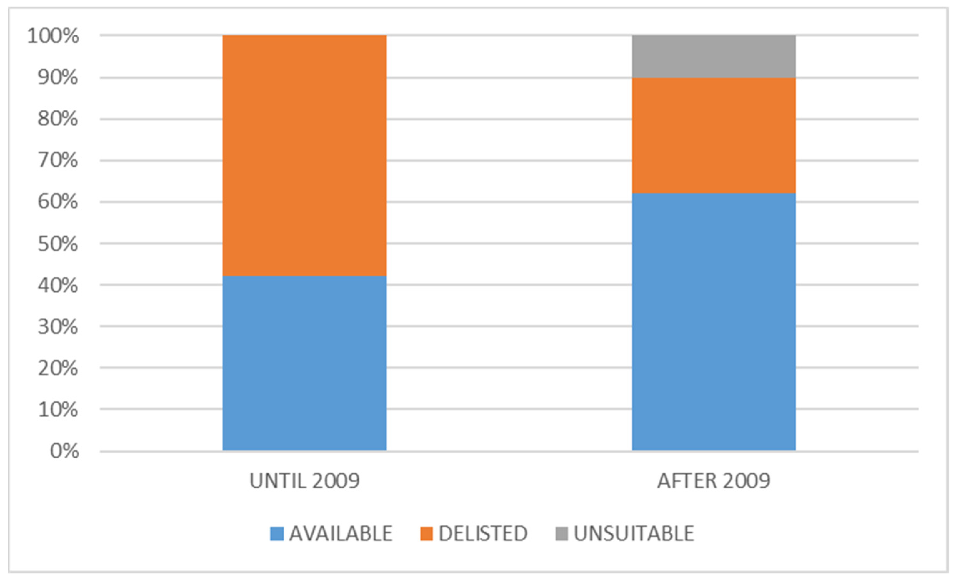
The Effect of the Recent Crisis on Value Creation of Greek Bidders

To understand the possible effect of the recent crisis on value creation, we test if the hypothesis of zero abnormal returns occurs both before and after the crisis. These tests are performed only for the trimmed sample. M&As are classified as “before crisis” if they were announced no later than 31 December 2009 and “after crisis” otherwise. These results are reported in Table 9.
Table 9 reveals some interesting findings. First, we note that M&As lead to zero abnormal returns before the crisis irrespective of how and when abnormal returns are measured, given that the corresponding hypothesis is never rejected (t-sig. < 0.05 in all cases in panel A). By contrast, our findings about M&As after the crisis are identical to those reported for the total trimmed sample, i.e., that daily abnormal returns are significantly less than zero on day −1 and day +4 and higher than zero on day +3 (t-sig. = 0. 0495 < 0.05) and day +5. Hence, it comes out that the recent crisis has changed the effect M&As have on value creation. The test regarding the median further supports this finding except for day +4, where the assumption of a zero median is not rejected at 5% (however, it would have been rejected at a slightly higher level, e.g., 7.5%). These median values and the results of the Wilcoxon signed-rank test for the trimmed sample are presented in Table 10.
The present study finds rather weak support for abnormal returns around M&A announcements except for the day preceding the event, where significant and negative abnormal returns are evidenced, contrary to the greatest part of relevant literature. It is worth noticing that three different statistical tests support this finding: are not only the mean and median abnormal returns significantly less than 0 one day before the event, but also, the percentage of M&As with negative abnormal returns significantly outperforms that of M&As with positive abnormal returns on the same day. It is also noted that, with minor exceptions, different definitions of event windows do not affect the conclusions about M&As’ effects on value creation: in most cases, the conclusions remain the same no matter which event window is considered. By contrast, we find strong evidence that non-normally distributed variables (abnormal returns) may, in most cases, be responsible for significantly altering findings regarding the role of M&As in value creation. Finally, our findings suggest that, in the pre-crisis era, there were zero abnormal returns on the day immediately preceding M&As, but after the crisis, M&As led to significant and negative abnormal returns one day before they were announced. Consequently, it is proven, although at a premature level, that the recent crisis increased the suspiciousness of investors toward M&As.

5. Conclusions

This study dealt with the issue of M&As’ effects on value creation at an empirical level. First, a brief theoretical background was formed with a focus on types, motives, and possible negative outcomes of M&As. Following this, existing relevant findings were examined to spot any controversies among relevant literature. By applying the event study approach, the present study sought to empirically investigate the effect of M&As on value creation before and after the recent crisis.
Theoretically, M&As are expected to provide several benefits depending on their type and, most importantly, the motivation behind them: economies of scale, increased negotiating power in terms of receiving finance, and enhancement of market share, are but a few. M&A benefits, however, are not a priori given as they exist problematic areas, especially at the level of planning and executing them, that, if not accounted for, may cause the exact opposite outcomes to occur. This explains, at least partially, the contradictory evidence regarding the effect of M&As. More precisely, part of the empirical findings so far reported implies a negative effect of M&As on value creation, especially for the shareholders of bidder firms.
To conduct the empirical analysis, the present study employed a sample of 84 M&As that took place in Greece from 2006 to 2015. Although the sample size is limited, mainly because of data unavailability, it is comparable to those employed by other studies regarding much larger markets. Looking at the distribution of M&As in Greece. To conduct the empirical analysis, the present study employed a sample of 84 M&As that took place in Greece from 2006 to 2015. Although the sample size is limited, mainly because of data unavailability, it is comparable to those employed by other studies regarding much larger markets. Looking at the distribution of M&As in Greece, it is evident that the recent crisis is associated with decreasing the number of such events after 2009. To examine the effect of M&As on value creation, two different event windows, namely a 3-day and an 11-day window, were considered. Abnormal returns were estimated based on the Market Model both on a daily and a cumulative basis. The empirical findings reported here suggest that M&As may not lead to abnormal returns around their announcement day, but they lead to abnormal (negative) returns for the day preceding them. We find strong evidence of this finding as it is supported by several statistical tests. From a methodological point of view, the event window definition does not seem to differentiate our conclusions. By contrast, the effect of non-normally distributed abnormal returns is strong to the point it could alter some of the conclusions drawn. As expected, the recent crisis altered the way M&As are perceived by the markets in that investors is not the way they were before the crisis, indifferent toward M&As and thought of such corporate events in a rather negative way (Shohaieb et al. 2022). Studying the impact of mergers and acquisitions (M&A) on shareholder wealth has several practical implications. First, it helps companies and investors make informed decisions regarding potential M&A deals by understanding their potential impact on shareholder value. This can lead to better negotiation and valuation of deals, as well as more accurate expectations for post-deal performance. Second, analyzing the effects of M&As on shareholder wealth can help regulators and policymakers understand the potential risks and benefits of such transactions and implement policies that promote the interests of shareholders. Finally, understanding the impact of M&As on shareholder wealth can inform the development of corporate governance practices and investor protection measures, which can help ensure that shareholders’ interests are safeguarded in these transactions.
Our findings may have implications for companies considering M&A activities, particularly during economic downturns. The study provides insights into how such activities can affect shareholder value during economic stress. However, a debate may suggest that companies that engage in M&A activities during economic downturns experience increased shareholder value. This could be due to factors such as increased consolidation and efficiency in the industry, as well as the potential for companies to acquire distressed assets at a lower cost during economic downturns; this study revealed that companies that engage in M&A activities during economic downturns tend to experience a decline in shareholder value. This could be due to various factors, such as increased uncertainty and risk associated with such activities during economic uncertainty. By understanding the potential impact of such activities on shareholder value, companies can make more informed decisions about whether and when to pursue M&A opportunities.
One of the limitations that are expected to affect this study’s findings, as well as those of similar ones, is related to the identification of the correct date of the M&A announcement. Although official documents were reviewed to record every M&A’s date of the announcement, there is no a priori certainty that stockholders were completely unaware of the forthcoming M&A. If this holds, abnormal returns may have occurred many days before the M&A was announced and, hence, may not be traced around its announcement. However, we deal with this issue by using two different event windows to examine the abnormal returns for a period that is very close to the M&A announcement and another one that expands more around the event.

Author Contributions

A.L., Data curation; A.L., Formal analysis; AL., Methodology; G.G. Project administration; G.G. Resources; A.L. and G.G., Software; M.E., Validation; A.L., Writing–original draft; M.E., Writing–review & editing. All authors have read and agreed to the published version of the manuscript.

Funding

This research received no external funding.

Data Availability Statement

The data supporting this study’s findings are available from the corresponding author upon reasonable request.

Conflicts of Interest

The authors declare no conflict of interest.

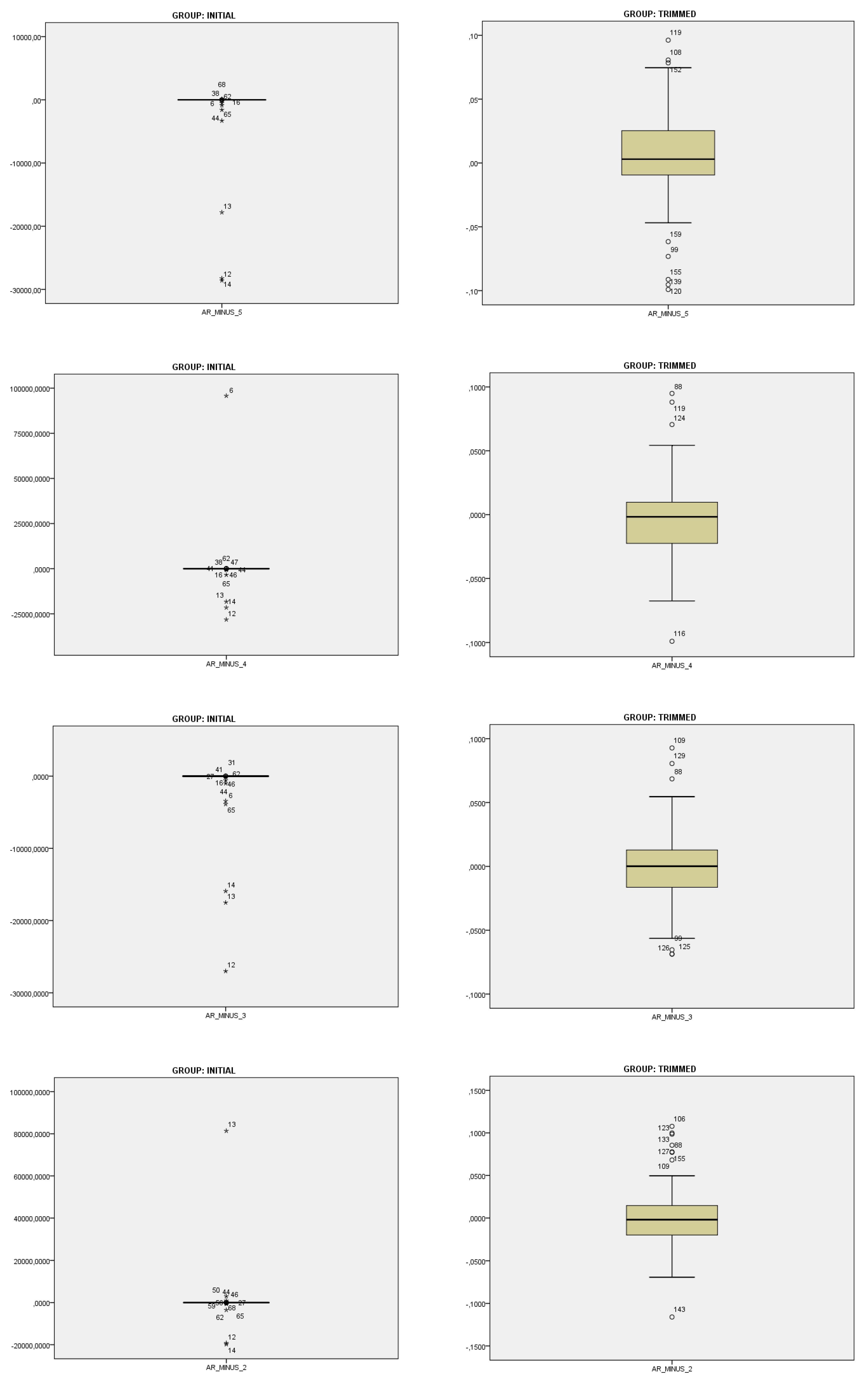
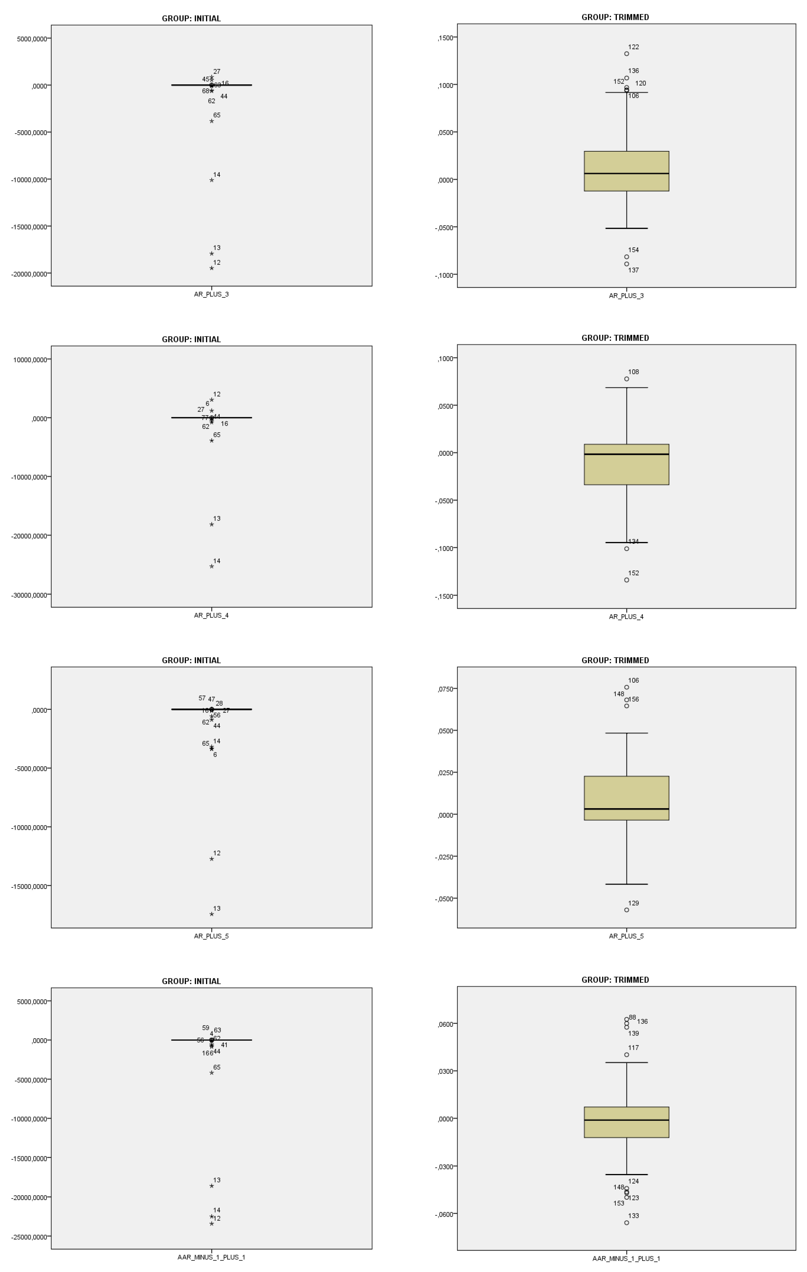
Appendix A. Boxplots of Initial and Trimmed Data

Jrfm 16 00199 g0a1aJrfm 16 00199 g0a1bJrfm 16 00199 g0a1cJrfm 16 00199 g0a1d

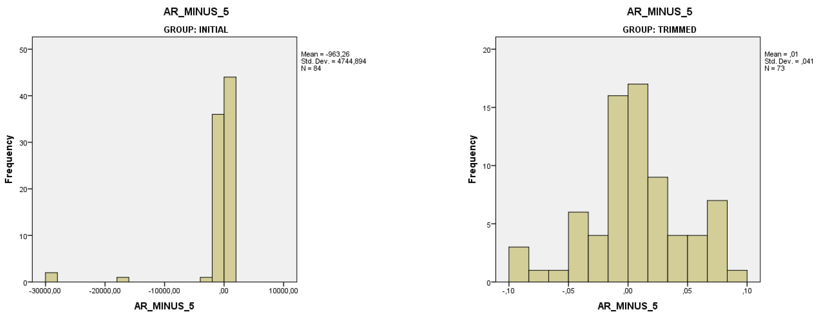
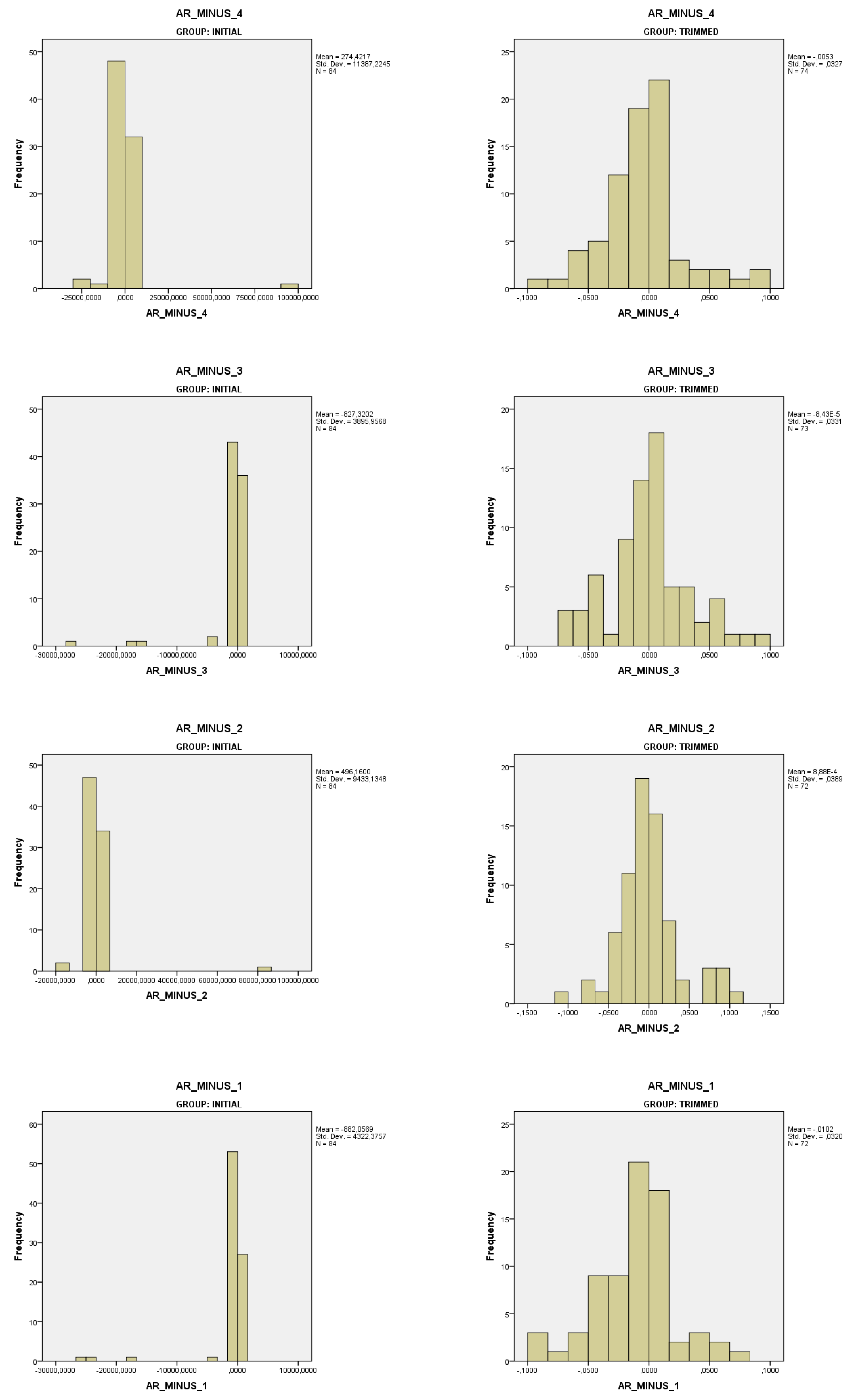
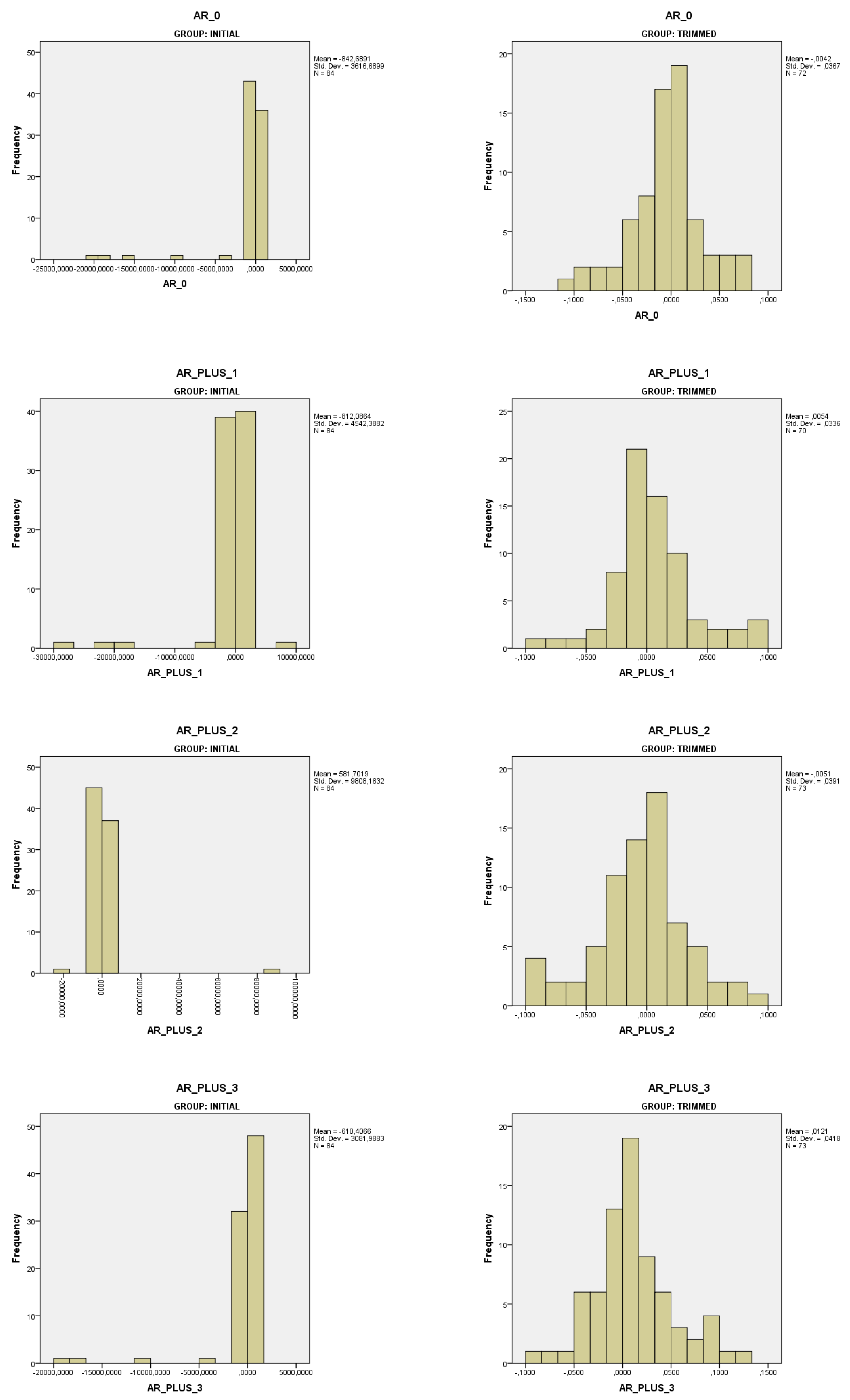
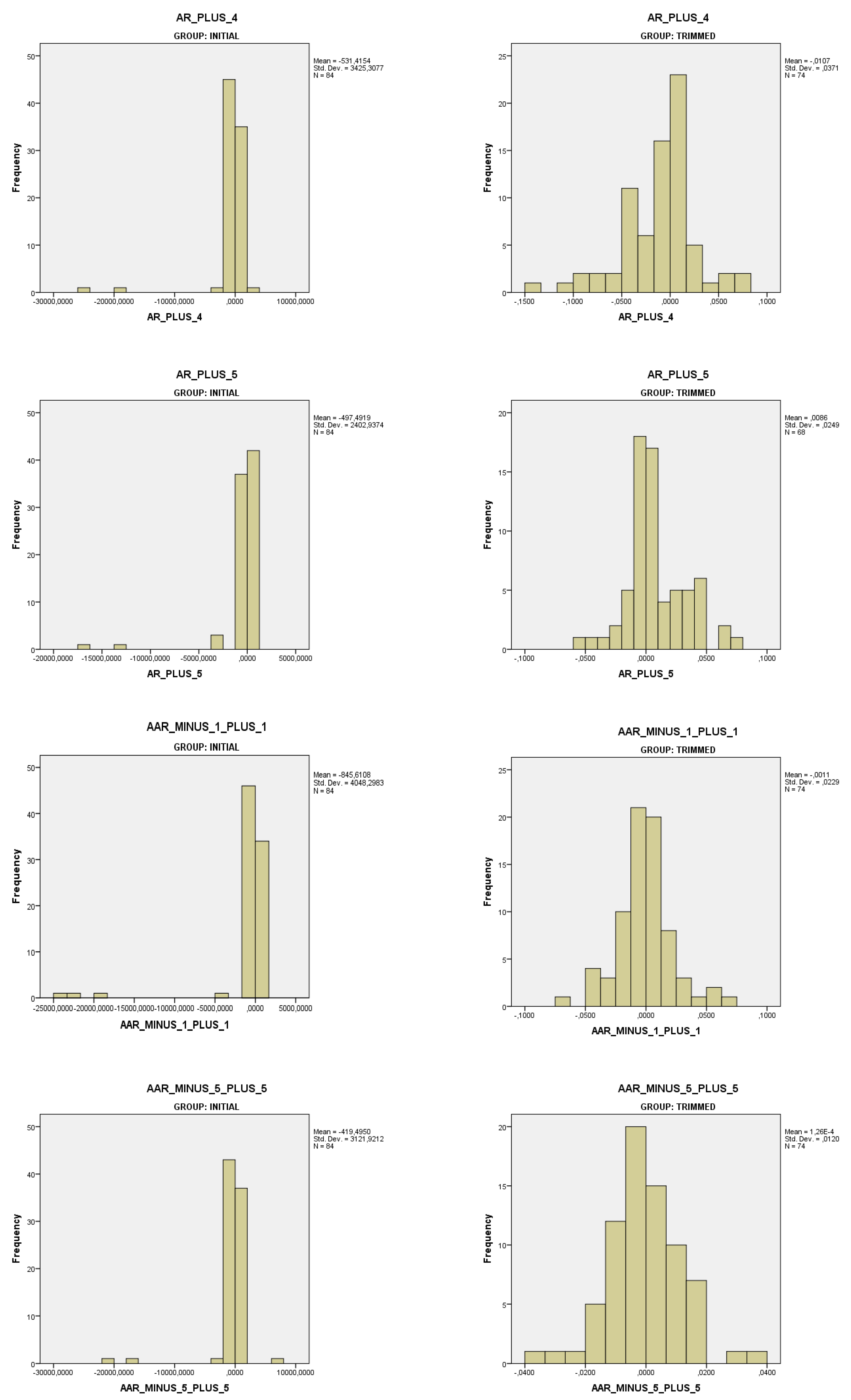
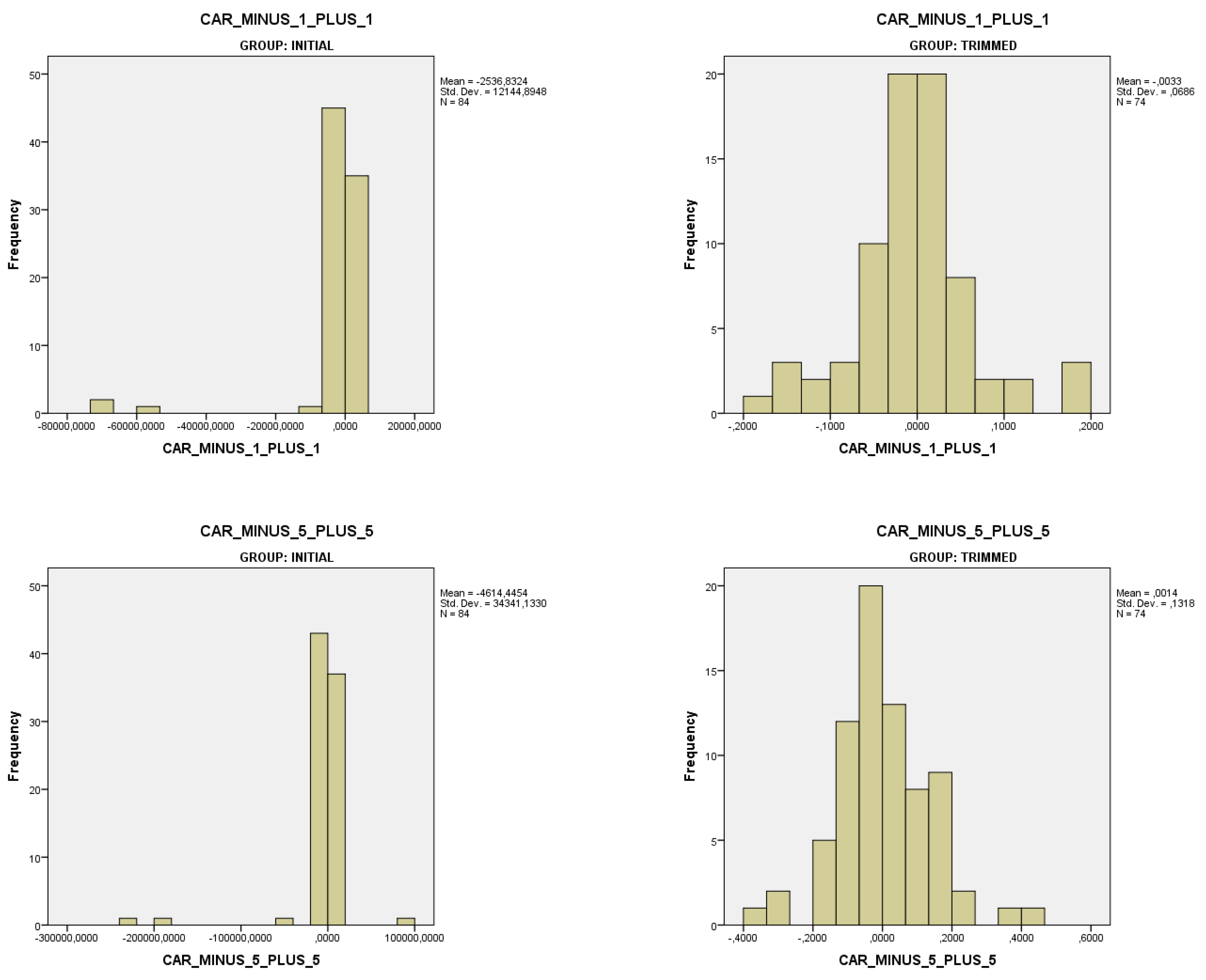
Appendix B. Histograms of Initial and Trimmed Data

Jrfm 16 00199 g0a2aJrfm 16 00199 g0a2bJrfm 16 00199 g0a2cJrfm 16 00199 g0a2dJrfm 16 00199 g0a2e

References

  1. Agrawal, Anup, Jeffrey F. Jaffe, and Gershon N. Mandelker. 1992. The post-merger performance of acquiring firms: A re-examination of an anomaly. Journal of Finance 47: 1605–21. [Google Scholar] [CrossRef]
  2. Antoniou, Antonios, Philippe Arbour, and Huainan Zhao. 2006. The Effects of the Cross-Correlation of Stock Returns on Post Merger Stock Performance. EFMA Basel Meetings Paper. Basel: EFMA Basel. [Google Scholar] [CrossRef]
  3. Arasa, Oirere David. 2020. Effect of Mergers and Acquisition on Shareholders Wealth of Listed Firms at Nairobi Securities Exchange, Kenya. Journal of Economics and Finance 11: 24–32. [Google Scholar]
  4. Asquith, Paul. 1983. Merger bids, uncertainty, and stockholder returns. Journal of Financial Economics 11: 51–83. [Google Scholar] [CrossRef]
  5. AT Kearney, Inc. 1999. Corporate Marriage: Blight or Bliss? A Monograph on Post-Merger Integration. Chicago: A.T. Kearney. [Google Scholar]
  6. Bradley, Michael, Anand Desai, and E. Han Kim. 1988. Synergistic gains from corporate acquisitions and their division between the stockholders of target and acquiring firms. Journal of Financial Economics 21: 3–40. [Google Scholar] [CrossRef] [Green Version]
  7. Brealey, Richard A., Stewart C. Myers, and Alan J. Marcus. 2001. Fundamentals of Corporate Finance, 3rd ed. New York: McGraw-Hill. [Google Scholar]
  8. Brown, Stephen J., and Jerold B. Warner. 1980. Measuring security price performance. Journal of Financial Economics 8: 205–58. [Google Scholar] [CrossRef]
  9. Brown, Stephen J., and Jerold B. Warner. 1985. Using daily stock returns: The case of event studies. Journal of Financial Economics 14: 3–31. [Google Scholar] [CrossRef]
  10. Chakrabarti, Rajesh, Swasti Gupta-Mukherjee, and Narayanan Jayaraman. 2005. Mars-Venus Marriages: Culture and Cross-Border M&A. SSRN Electronic Journal 40: 216–36. [Google Scholar] [CrossRef]
  11. Chang, Saeyoung. 2002. Takeovers of Privately Held Targets, Methods of Payment, and Bidder Returns. Journal of Finance 53: 773–84. [Google Scholar] [CrossRef]
  12. Dodd, Peter. 1980. Merger proposals management discretion and stockholder wealth. Journal of Financial Economics 8: 105–38. [Google Scholar] [CrossRef]
  13. Dodd, Peter, and Richard Ruback. 1977. Tender offers and stockholder returns: An empirical analysis. Journal of Financial Economics 5: 351–73. [Google Scholar] [CrossRef]
  14. Eckbo, B. Espen. 1983. Horizontal mergers, collusion, and stockholder wealth. Journal of Financial Economics 11: 241–73. [Google Scholar] [CrossRef]
  15. Fama, Eugene F., Lawrence Fisher, Michael C. Jensen, and Richard Roll. 1969. The adjustment of stock prices to new information. International Economic Review 10: 1–21. [Google Scholar] [CrossRef]
  16. Franks, Julian R., and Robert S. Harris. 1989. Shareholder wealth effects of corporate takeovers: The UK experience 1955–85. Journal of Financial Economics 23: 195–224. [Google Scholar] [CrossRef]
  17. Goergen, Marc, and Luc Renneboog. 2004. Shareholder Wealth Effects of European Domestic and Cross-Border Takeover Bids. European Financial Management 10: 9–45. [Google Scholar] [CrossRef]
  18. Heaton, James B. 2002. Managerial Optimism and Corporate Finance. Financial Management 31: 33–45. [Google Scholar] [CrossRef]
  19. Higson, Chris, and Jamie Elliott. 1998. Post-takeover returns: The UK evidence. Journal of Empirical Finance 5: 27–46. [Google Scholar] [CrossRef]
  20. Malatesta, Paul H. 1983. The wealth effect of merger activity and the objective function of merging firms. Journal of Financial Economics 11: 155–82. [Google Scholar] [CrossRef]
  21. Martynova, M., and L. Renneboog. 2006. Mergers and Acquisitions in Europe. ECGI Working Paper N.114/2006. Available online: https://core.ac.uk/reader/6651890 (accessed on 4 March 2023).
  22. Monga, Suman. 2021. Impact of Mergers and Acquisitions Announcement on Shareholders’ Wealth: Evidence from Indian Corporate Sector. Turkish Online Journal of Qualitative Inquiry 12: 10. [Google Scholar]
  23. Petmezas, D. 2009. What Drives Acquisitions? Journal of Multinational Financial Management 19: 54–74. [Google Scholar] [CrossRef] [Green Version]
  24. Protopapas, G. P., N. G. Travlos, and N. V. Tsagarakis. 2003. Mergers and Acquisitions in Greece: Stock price Reaction of Acquiring and Target Firms. Piraeus: SPOUDAI, vol. 53, pp. 80–104. [Google Scholar]
  25. Rani, Neelam, Surendra S. Yadav, and P. K. Jain. 2013. Impact of Corporate Governance Score on Abnormal Returns of Mergers and Acquisitions. Procedia Economics and Finance 5: 637–46. [Google Scholar] [CrossRef] [Green Version]
  26. Shohaieb, D., M. Elmarzouky, and K. Albitar. 2022. Corporate governance and diversity management: Evidence from a disclosure perspective. International Journal of Accounting & Information Management, ahead-of-print. [Google Scholar]
  27. Sudarsanam, Sudi, Peter Holl, and Ayo Salami. 1996. Shareholder wealth gains in mergers: Effect of synergy and ownership structure. Journal of Business Finance and Accounting 23: 673–98. [Google Scholar] [CrossRef]
  28. Tampakoudis, Ioannis, and Evgenia Anagnostopoulou. 2020. The effect of mergers and acquisitions on environmental, social and governance performance and market value: Evidence from EU acquirers. Business Strategy and the Environment 29: 1865–75. [Google Scholar] [CrossRef]
  29. Tampakoudis, Ioannis, Michail Nerantzidis, Gabriel Eweje, and Stergios Leventis. 2022. The impact of gender diversity on shareholder wealth: Evidence from European bank M&A. Journal of Financial Stability 60: 101020. [Google Scholar]
  30. Teti, Emanuele, and Stefano Tului. 2020. Do mergers and acquisitions create shareholder value in the infrastructure and utility sectors? Analysis of market perceptions. Utilities Policy 64: 101053. [Google Scholar] [CrossRef]
  31. Varmaz, Armin, and Jonas Laibner. 2016. Announced versus canceled bank mergers and acquisitions—Evidence from the European banking industry. The Journal of Risk Finance 17: 510–44. [Google Scholar] [CrossRef]
  32. Wasilewski, Mirosław, Serhiy Zabolotnyy, and Dmytro Osiichuk. 2021. Characteristics and shareholder wealth effects of mergers and acquisitions involving European renewable energy companies. Energies 14: 7126. [Google Scholar] [CrossRef]
  33. Weber, Roberto A., and Colin F. Camerer. 2003. Cultural Conflict and Merger Failure: An Experimental Approach. Management Science 49: 400–15. [Google Scholar] [CrossRef] [Green Version]
Figure 1. Distribution of M&As with known dates during 2006–2015 in Greece.
Jrfm 16 00199 g001
Figure 2. Data availability until and after 2009.
Jrfm 16 00199 g002
Table 1. Name of variables and Notations.
NotationsName of the Variables
AR_MINUS_5the average abnormal return 5 days before the event
AR_MINUS_4the average abnormal return 4 days before the event
AR_MINUS_3the average abnormal return 3 days before the event
AR_MINUS_2the average abnormal return 2 days before the event
AR_MINUS_1the average abnormal return 1 day before the event
AR_0the average abnormal return 5 on the day of the event
AR_PLUS_1the average abnormal return 1 day after the event
AR_PLUS_2the average abnormal return 2 days after the event
AR_PLUS_3the average abnormal return 3 days after the event
AR_PLUS_4the average abnormal return 4 days after the event
AR_PLUS_5the average abnormal return 5 days after the event
CAR_MINUS_1_PLUS_1the cumulative average abnormal return 3 days around the event
CAR_MINUS_5_PLUS_5the cumulative abnormal return 11 days around the event
Table 2. Normality tests—Initial data set.
Kolmogorov–SmirnovShapiro–Wilk
StatisticsdfSig.StatisticsdfSig.
AR_MINUS_50.487840.0000.206840.000
AR_MINUS_40.498840.0000.193840.000
AR_MINUS_30.490840.0000.222840.000
AR_MINUS_20.485840.0000.172840.000
AR_MINUS_10.490840.0000.206840.000
AR_00.496840.0000.246840.000
AR_PLUS_10.482840.0000.250840.000
AR_PLUS_20.500840.0000.154840.000
AR_PLUS_30.495840.0000.220840.000
AR_PLUS_40.488840.0000.195840.000
AR_PLUS_50.480840.0000.215840.000
CAR_MINUS_1_PLUS_10.489840.0000.211840.000
CAR_MINUS_5_PLUS_50.494840.0000.226840.000
Table 3. Normality tests after deleting extreme outliers.
Kolmogorov-SmirnovShapiro-Wilk
StatisticsdfSig.StatisticsdfSig.
AR_MINUS_50.136730.0020.963730.031
AR_MINUS_40.117740.0140.953740.007
AR_MINUS_30.107730.0390.966730.046
AR_MINUS_20.138720.0020.930720.001
AR_MINUS_10.121720.0110.959720.019
AR_00.112720.0250.962720.029
AR_PLUS_10.116700.0210.950700.007
AR_PLUS_20.087730.2000.974730.135
AR_PLUS_30.111730.0260.961730.022
AR_PLUS_40.135740.0020.943740.002
AR_PLUS_50.163680.0000.947680.006
CAR_MINUS_1_PLUS_10.119740.0110.946740.003
CAR_MINUS_5_PLUS_50.097740.0830.969740.065
Table 4. Descriptive statistics.
NMeanMedianStd. DeviationSkewnessKurtosis
PANEL A: INITIAL
AR_MINUS_584−963.2620.0014744.894−5.32727.983
AR_MINUS_484274.422−0.00711,387.2256.93961.632
AR_MINUS_384−827.320−0.0033895.957−5.42930.552
AR_MINUS_284496.160−0.0029433.1357.54567.428
AR_MINUS_184−882.057−0.0074322.376−5.19526.350
AR_084−842.689−0.0053616.690−4.59020.539
AR_PLUS_184−812.086−0.0014542.388−5.01427.042
AR_PLUS_284581.702−0.0039808.1637.85271.000
AR_PLUS_384−610.4070.0043081.988−5.39029.196
AR_PLUS_484−531.415−0.0033425.308−6.34941.485
AR_PLUS_584−497.4920.0002402.937−6.00137.627
AAR_MINUS_1_PLUS_184−845.611−0.0034048.298−5.07224.837
AAR_MINUS_5_PLUS_584−419.495−0.0013121.921−5.30133.097
CAR_MINUS_1_PLUS_184−2536.832−0.00912,144.895−5.07224.837
CAR_MINUS_5_PLUS_584−4614.445−0.01334,341.133−5.30133.097
PANEL B: TRIMMED
AR_MINUS_5730.0060.0030.041−0.2430.521
AR_MINUS_474−0.005−0.0020.0330.3711.856
AR_MINUS_3730.0000.0000.0330.2500.572
AR_MINUS_2720.001−0.0020.0390.5251.769
AR_MINUS_172−0.010−0.0050.032−0.1271.297
AR_072−0.004−0.0010.037−0.2530.837
AR_PLUS_1700.0050.0020.0340.3121.333
AR_PLUS_273−0.005−0.0020.039−0.2120.682
AR_PLUS_3730.0120.0060.0420.5320.767
AR_PLUS_474−0.011−0.0020.037−0.6491.608
AR_PLUS_5680.0090.0030.0250.3930.788
AAR_MINUS_1_PLUS_174−0.001−0.0010.0230.1751.717
AAR_MINUS_5_PLUS_5740.000−0.0010.0120.1291.767
CAR_MINUS_1_PLUS_174−0.003−0.0030.0690.1751.717
CAR_MINUS_5_PLUS_5740.001−0.0110.1320.1291.767
Table 5. t-test for mean difference of daily abnormal returns from day −5 to day +5.
tdfSig.
(2 Tailed)
Mean
Difference
95% Confidence Interval
of the Difference
LowerUpper
PANEL A: INITIAL
AR_MINUS_5−1.861830.066−963.262−1992.96866.443
AR_MINUS_40.221830.826274.422−2196.7582745.601
AR_MINUS_3−1.946830.055−827.320−1672.79518.154
AR_MINUS_20.482830.631496.160−1550.9562543.276
AR_MINUS_1−1.870830.065−882.057−1820.07055.956
AR_0−2.135830.036−842.689−1627.559−57.819
AR_PLUS_1−1.639830.105−812.086−1797.845173.672
AR_PLUS_20.544830.588581.702−1546.8002710.204
AR_PLUS_3−1.815830.073−610.407−1279.23958.426
AR_PLUS_4−1.422830.159−531.415−1274.753211.922
AR_PLUS_5−1.898830.061−497.492−1018.96123.977
PANEL B: TRIMMED
AR_MINUS_51.194720.2360.006−0.0040.015
AR_MINUS_4−1.389730.169−0.005−0.0130.002
AR_MINUS_3−0.022720.9830.000−0.0080.008
AR_MINUS_20.194710.8470.001−0.0080.010
AR_MINUS_1−2.701710.009−0.010−0.018−0.003
AR_0−0.964710.338−0.004−0.0130.004
AR_PLUS_11.357690.1790.005−0.0030.013
AR_PLUS_2−1.111720.270−0.005−0.0140.004
AR_PLUS_32.468720.0160.0120.0020.022
AR_PLUS_4−2.476730.016−0.011−0.019−0.002
AR_PLUS_52.841670.0060.0090.0030.015
Table 6. t-test for mean difference of cumulative abnormal returns from day −1 to day +1 and from day −5 to day +5.
tdfSig.
(2 Tailed)
Mean
Difference
95% Confidence Interval
of the Difference
LowerUpper
PANEL A: INITIAL
CAR_MINUS_1_PLUS_1−1.914830.059−2536.832−5172.43698.771
CAR_MINUS_5_PLUS_5−1.232830.222−4614.445−12,066.9282838.037
PANEL B: TRIMMED
CAR_MINUS_1_PLUS_1−0.419730.676−0.003−0.0190.013
CAR_MINUS_5_PLUS_50.091730.9280.001−0.0290.032
Table 7. Wilcoxon signed-rank test for median daily, average, and cumulative abnormal returns in the initial and trimmed sample (test value = 0).
INITIALTRIMMED
NMedianW-Sig.NMedianW-Sig.
AR_MINUS_5840.0010.925730.0030.149
AR_MINUS_484−0.0070.00474−0.0020.070
AR_MINUS_384−0.0030.035730.0000.832
AR_MINUS_284−0.0020.40972−0.0020.559
AR_MINUS_184−0.0070.00072−0.0050.005
AR_084−0.0050.03572−0.0010.394
AR_PLUS_184−0.0010.844700.0020.245
AR_PLUS_284−0.0030.10273−0.0020.351
AR_PLUS_3840.0040.230730.0060.029
AR_PLUS_484−0.0030.02174−0.0020.055
AR_PLUS_5840.0000.779680.0030.013
CAR_MINUS_1_PLUS_184−0.0090.02374−0.0030.548
CAR_MINUS_5_PLUS_584−0.0130.59374−0.0110.848
Table 8. Proportion of cases with negative and positive abnormal returns and χ2 tests.
CountsPercentagesχ2 Test
NegativePositiveNegativePositiveStatisticsSig.
AR_MINUS_5_DUMMY493558%42%2.3330.127
AR_MINUS_4_DUMMY513361%39%3.8570.050
AR_MINUS_3_DUMMY473756%44%1.1900.275
AR_MINUS_2_DUMMY473756%44%1.1900.275
AR_MINUS_1_DUMMY562867%33%9.3330.002
AR_0_DUMMY483657%43%1.7140.190
AR_PLUS_1_DUMMY444052%48%0.1900,663
AR_PLUS_2_DUMMY463855%45%0.7620.383
AR_PLUS_3_DUMMY354942%58%2.3330.127
AR_PLUS_4_DUMMY483657%43%1.7140.190
AR_PLUS_5_DUMMY424250%50%0.0001.000
CAR_MINUS_1_PLUS_1_DUMMY493558%42%2.3330.127
CAR_MINUS_5_PLUS_5_DUMMY463855%45%0.7620.383
Table 9. t-test for mean difference of daily, average, and cumulative abnormal returns before and after the crisis.
tdfSig.
(2 Tailed)
Mean
Difference
95% Confidence Interval
of the Difference
LowerUpper
PANEL A: BEFORE CRISIS
AR_MINUS_50.010300.9920.000−0.0120.012
AR_MINUS_4−1.107310.277−0.007−0.0190.005
AR_MINUS_3−0.056310.9560.000−0.0130.012
AR_MINUS_20.107310.9150.001−0.0130.014
AR_MINUS_1−0.437310.665−0.003−0.0150.010
AR_00.117310.9080.001−0.0130.014
AR_PLUS_11.800300.0820.012−0.0020.025
AR_PLUS_2−0.466310.645−0.003−0.0140.009
AR_PLUS_31.394310.1730.009−0.0040.021
AR_PLUS_4−1.076310.290−0.007−0.0210.006
AR_PLUS_51.666300.1060.008−0.0020.017
CAR_MINUS_1_PLUS_11.499310.1440.013−0.0050.031
CAR_MINUS_5_PLUS_51.097310.2810.023−0.0200.065
PANEL B: AFTER CRISIS
AR_MINUS_51.391410.1720.010−0.0040.024
AR_MINUS_4−0.863410.393−0.004−0.0150.006
AR_MINUS_30.023400.9820.000−0.0100.010
AR_MINUS_20.160390.8730.001−0.0120.014
AR_MINUS_1−3.599390.001−0.016−0.025−0.007
AR_0−1.423390.163−0.008−0.0200.003
AR_PLUS_10.077380.9390.000−0.0100.010
AR_PLUS_2−1.012400.318−0.007−0.0210.007
AR_PLUS_32.025400.0500.0150.0000.029
AR_PLUS_4−2.353410.023−0.013−0.025−0.002
AR_PLUS_52.309360.0270.0090.0010.018
CAR_MINUS_1_PLUS_1−1.323410.193−0.016−0.0400.008
CAR_MINUS_5_PLUS_5−0.691410.494−0.015−0.0590.029
Table 10. Non-parametric tests.
Before CrisisAfter Crisis
NMedianW-Sig.NMedianW-Sig.
AR_MINUS_5310.0000.814420.0080.063
AR_MINUS_432−0.0070.064420.0010.427
AR_MINUS_332−0.0010.837410.0010.964
AR_MINUS_232−0.0020.61440−0.0010.657
AR_MINUS_132−0.0040.41140−0.0090.002
AR_032−0.0010.911400.0000.313
AR_PLUS_1310.0080.09239−0.0010.900
AR_PLUS_232−0.0010.70841−0.0020.361
AR_PLUS_3320.0080.286410.0060.045
AR_PLUS_4320.0000.41142−0.0040.071
AR_PLUS_5310.0000.248370.0040.020
AAR_MINUS_1_PLUS_1320.0030.21042−0.0040.086
AAR_MINUS_5_PLUS_5320.0000.58842−0.0010.413
CAR_MINUS_1_PLUS_1320.0100.21042−0.0110.086
CAR_MINUS_5_PLUS_5320.0020.58842−0.0140.413
Disclaimer/Publisher’s Note: The statements, opinions and data contained in all publications are solely those of the individual author(s) and contributor(s) and not of MDPI and/or the editor(s). MDPI and/or the editor(s) disclaim responsibility for any injury to people or property resulting from any ideas, methods, instructions or products referred to in the content.

