Pricing Multi-Asset Bermudan Commodity Options with Stochastic Volatility Using Neural Networks

Abstract

It has been recognized that volatility in commodity markets fluctuates significantly depending on the demand–supply relationship and geopolitical risk, and that risk and financial management using multivariate derivatives are becoming more important. This study illustrates an application of multi-layered neural networks for multi-dimensional Bermudan option pricing problems assuming a multi-asset stochastic volatility model in commodity markets. In addition, we aim to identify continuation value functions for these option pricing problems by implementing smooth activation functions in the neural networks and evaluating their accuracy compared with other activation functions or regression techniques. First, we express the underlying asset dynamics using the multi-asset stochastic volatility model with mean reversion properties in the commodity market and formulate the multivariate Bermudan commodity option pricing problem. Subsequently, we apply multi-layer perceptrons in the neural network to represent the continuation value functions of Bermudan commodity options, wherein the entire neural network is trained using the least-squares Monte Carlo simulation method. Finally, we perform numerical experiments and demonstrate that applications of neural networks for Bermudan options in a multi-dimensional commodity market achieve sufficient accuracy with regard to various aspects, including changing the exercise dates, the number of layers/neurons, and the dimension of the problem.

1. Introduction

In commodity markets, typical products include directional trades such as futures and forwards, which establish an obligation to purchase or sell an underlying commodity in the future (Clark 2014). As essential tools for managing risks from these contracts, which may consist of multiple underlying assets, there are various options contracts that provide a right to trade the underlying commodity under a specified condition. In this study, we focus on early-exercisable options on multiple underlying assets in commodity markets, i.e., multivariate Bermudan commodity options.

Solving Bermudan commodity option pricing problems with multiple underlying assets and factors is challenging because computational efforts grow exponentially in tandem with the problem dimension in general, which is determined by the number of assets and factors. However, the improvement of algorithms and the rapid growth of computational power have led to a remarkable surge of interest in computational science in recent years. Currently, a wide variety of machine learning algorithms, such as deep learning and neural networks, are successfully employed for classification, regression, clustering, or dimensionality reduction tasks and are applied for large-sized and high-dimensional data in various areas. In this study, we develop a new Bermudan commodity option algorithm via multi-layered neural networks and show its efficiency and effectiveness based on the multi-asset commodity market model with stochastic volatility, wherein significant changes in volatility may be observed according to the demand–supply relationship and geopolitical conditions in commodity markets.

An important feature of Bermudan options is that they can be exercised early, with their value being determined by whether or not they are exercised before maturity. In other words, the option holder must decide whether to continue holding the option or immediately exercise it at a prespecified period. In this situation, it is crucial to determine the continuation value, i.e., the value of holding the option until the next exercise window. Such a continuation value may be given as the discounted conditional expectation of the remaining option value on one step ahead under a risk-neutral probability measure, which generally has no explicit boundary conditions. Moreover, the conditional expectation providing the continuation value is an unknown (possibly nonlinear and complex) multivariate function whose dimensions depend on the number of underlying factors; hence, an exact (yet still approximate) computation involves high-dimensional discrete grids concerning state variables and is quite difficult to solve.

To price early-exercisable options with estimations of continuation value functions, Longstaff and Schwartz (2001) proposed a simple yet powerful numerical method involving a regression-based functional estimation using simulated sample paths known as the least-squares Monte Carlo (LSMC) method. Since then, several studies have examined the application of neural networks (or machine learning methods) for estimating continuation value functions in option pricing based on the LSMC method. For American options’ pricing, Haugh and Kogan (2004) applied a neural network with one hidden layer for valuation, whereas Kohler et al. (2010) proved price consistency and convergence with multiple payoff types. Lapeyre and Lelong (2021) gave several numerical examples of Bermudan options and proved convergence. There are additional examples, e.g., the 5000 assets rainbow option (Becker et al. 2021) and expected exposures (Andersson and Oosterlee 2021). Furthermore, other machine learning algorithms have been used for early-exercisable options, e.g., radial basis functions (Ballestra and Pacelli 2013), nearest-neighbor (Feng et al. 2013), deep learning (Becker et al. 2020; Liang et al. 2021), unsupervised learning (Salvador et al. 2020), and reinforcement learning (Li 2022), as well as the support vector machine (Lin and Almeida 2021). Moreover, numerical approaches have also been used, including stochastic kriging metamodels (Ludkovski 2018), high-dimensional partial differential equations (Sirignano and Spiliopoulos 2018), and backward stochastic differential equations (Chen and Wan 2021). Furthermore, there are other applications of neural networks in the finance field, e.g., extending the feature set (Montesdeoca and Niranjan 2016), the calculation of implied volatilities (Liu et al. 2019), and decision-making (Puka et al. 2021). A comprehensive review of these methods was conducted by Ruf and Wang (2020).

Although this study shares the same ideas as the aforementioned studies—in particular, as in Lapeyre and Lelong (2021), given that a multi-layer perceptron (MLP) is applied in the neural network—it is worthwhile to mention that our study may be considered novel in several aspects: We illustrate an algorithm for estimating the continuation values of multi-asset Bermudan commodity options with stochastic volatility features, whereby a smooth activation function, such as the sigmoid function, is applied in the MLP to reflect the smoothness of conditional expectations regarding state variables. The smoothness of functions to represent conditional expectations is key in this study. In the Markovian setting, the conditional probability density functions are usually smooth given state variables; thus, conditional expectations are smooth functions. Therefore, the target continuation value function is smooth, and we can expect a better fit to the target function by using a smooth activation function in the MLP. This is in contrast with more commonly used piecewise linear functions such as the leaky ReLU function applied in the numerical experiments by Lapeyre and Lelong (2021), wherein the fitting function may not be smooth but only piecewise smooth. (Note that, in a similar context with the smoothness of estimated functions, Yamada (2012, 2017) applied the generalized additive model to calculate smooth functions for conditional expectations in multivariate hedging problems with European and Bermudan options.) Additionally, we applied more sophisticated techniques such as the resampling procedure and early stopping to improve the computational efficiency and avoid possible biases in pricing or overfitting for optimal learning (see Section 3.2 and the numerical experiments).

While several neural network/machine learning models for option pricing exist, we believe that, for this type of research, the current methodologies, along with developed computational algorithms, need to be combined with existing techniques using the currently available computational environment. In this context, the choice of problem and methodology choice is important, as is the approach to the problem and how to perform the numerical experiments. The combination of multi-asset commodity options with stochastic volatility and recently developed neural network techniques (including the computational environment and software) is meaningful since commodity markets are largely volatile, and this volatility may change over time. Moreover, the multi-asset Bermudan commodity options with stochastic volatility, to the best of our knowledge, have not been previously considered despite the problem’s importance. It should become more challenging in numerical calculations to configure multiple underlying assets that recognize mean-reverting dynamics and solve boundary conditions with stochastic factors (see, e.g., Hahn and Dyer 2008 and Ball and Roma 1994).

The present study implements a multi-layered neural network and examines its efficiency and effectiveness for multi-asset Bermudan commodity option pricing problems with stochastic volatility. First, we formulate the multi-asset commodity market with stochastic volatility, wherein individual asset price dynamics are expressed as a two-factor model by combining a well-known commodity model by Schwartz (1997) with Heston’s stochastic volatility model (Heston 1993). Next, we apply MLPs in the neural network to represent the continuation value functions in Bermudan option pricing, whereby the entire neural network is trained using LSMC simulations. We perform numerical experiments to compare the continuation value function accuracy in response to changing the exercise dates, the number of layers/neurons, and the dimension of the problem. We also compare the relationship between the continuation values and network configurations.

The outline of this article is as follows. Section 2 gives an introduction to the commodity option structure adopted in this study and the formulation of the multi-dimensional Bermudan option problem. Section 3 describes the configuration of neural networks, a multi-dimensional asset model with stochastic volatility, and a Bermudan options pricing procedure for learning and valuation via Monte Carlo sample paths. Section 4 presents the numerical results of the Bermudan option prices and compares the accuracy of the continuation value surfaces. Section 5 summarizes the analysis results and discussions. Lastly, Section 6 concludes this study.

2. Pricing Multi-Asset Bermudan Commodity Options with Stochastic Volatility

In this section, we introduce early-exercisable commodity options and formulate the problem of pricing multi-asset Bermudan commodity options with stochastic volatility.

2.1. Early-Exercisable Commodity Options

As stated earlier, in commodity markets, typical products include plain directional trades such as future and forward contracts, which establish an obligation to buy or sell a particular commodity asset at a specified price in the future (Clark 2014). Depending on the terminal values of commodity assets, holding these contracts may lead to a loss or profit for the contractor, while a large loss is particularly undesirable for the holder; furthermore, the possibility of a large profit may be pursued. Such opportunities are realized using options contracts, giving a right to purchase or sell an underlying commodity asset with a prespecified strike price in the future.

Among the many types of options used as hedging tools in commodity markets, early-exercisable options provide additional flexibility regarding exercise timing and are considered useful for hedgers, in practice. Traditionally, such options are characterized as American options; however, in the context of exotic options, Bermudan options have similar flexibility. These options allow holders to exercise them early, although only on specific dates before maturity; thus, the option holder must decide whether to continue holding the option or immediately exercise it during the exercisable period. However, such continuation value is usually unknown because it depends on future option values on specific exercisable dates. Therefore, it is paramount to determine the continuation values for Bermudan options. The objective of this study is to evaluate computational performance (including the accuracy of continuation value estimation) for pricing multi-asset Bermudan commodity options via multi-layered neural networks.

2.2. Multi-Dimensional Bermudan Option Pricing Problem

In this subsection, we describe the multi-dimensional Bermudan option pricing problem, following Lapeyre and Lelong (2021). Given a complete filtered probability space ($\Omega$, $ℱ$, ${\left({ℱ}_t\right)}_{0\le t\le T}$, $\mathbb{P}$) with a finite time horizon $T>0$, we assume that a set of underlying assets is modeled via a multifactored process ${\left(X_t\right)}_{0\le t\le T}$ adapted to the filtration, ${\left({ℱ}_t\right)}_{0\le t\le T}$, and that $\mathbb{P}$ is an associated risk-neutral measure. We consider a Bermudan option with exercise dates $0=T_0\le T_1<T_2<\dots <T_N=T$ and a discrete-time payoff process $P_{T_n}$ if exercised at times ${\left(T_n\right)}_{0\le n\le N}$, where $P_{T_n}$ is specified as a function of $X_{T_n}$. Then, Bermudan option prices $Z_{T_n}$ are computed using the following recursive equation:

$$\{\begin{array}{c}{Z}_{T_N}=P_{T_N}\\ Z_{T_n}=max\left(P_{T_n},e^{-r{\mathsf{\delta }}_{T_n}}\mathbb{E}\left[Z_{T_{n+1}}|{ℱ}_{T_n}\right]\right) , 0\le n\le N-1\end{array}$$

(1)

where $\mathbb{E}$ denotes the expectation under the risk-neutral probability measure $\mathbb{P}$ with the risk-free interest rate $r$ and the interval between $T_{n-1}$ and $T_n$ as ${\mathsf{\delta }}_{T_n}$. Furthermore, assuming that ${\left(X_t\right)}_{0\le t\le T}$ is a multi-dimensional Markov process, there exists a measurable function ${\Phi }_n: {ℝ}^{d_x}\to ℝ$, such that:

$$e^{-r{\mathsf{\delta }}_{T_n}}\mathbb{E}\left[Z_{T_{n+1}}|{ℱ}_{T_n}\right]=e^{-r{\mathsf{\delta }}_{T_n}}\mathbb{E}\left[Z_{T_{n+1}}|X_{T_n}\right]={\Phi }_n\left(X_{T_n}\right) , 0\le n\le N-1.$$

(2)

Herein, we refer to ${\Phi }_n$ as a continuation value function in this paper.

Note that finding the exact ${\Phi }_n$ is difficult; alternatively, one may identify a function $f_n$ to minimize the following quantity,

$$\mathbb{E}\left[{\left|e^{-r{\mathsf{\delta }}_{T_n}}{Z}_{T_{n+1}}-f_n\left(X_{T_n}\right)\right|}^2\right],$$

(3)

over a parametrized set of functions 𝕭. If all (real-valued) square-integrable measurable functions are searched to minimize Equation (3), it turns out that the function ${\Phi }_n$ providing the conditional expectation in Equation (2) is achieved via an optimizer. However, there is a trade-off between the generality of a set of functions and the efficiency of computation. Additionally, computational tractability depends on the methodology to solve the optimization problem.

2.3. Multi-Asset Commodity Market Model with Stochastic Volatility

This study employs a multivariate commodity market model consisting of multiple underlying assets with stochastic volatility for the Bermudan option problem. To this end, we adopt a stochastic volatility model for the mean-reverting commodity dynamics (Schwartz 1997) and expand it to the multi-asset case.

Consider the Bermudan option problem with $n$ underlying assets at time $t$, $S_{i,t}, i=1,\dots , l$, the $i$-th price dynamics of which are governed by the following two-dimensional stochastic differential equations (SDEs):

$$\begin{gathered} d{S}_{i,t}={\kappa }_{S_i}\left({\mu }_i-\ln S_{i,t}\right)S_{i,t}dt+\sqrt{v_{i,t}}{S}_{i,t} d{W}_{S_i,t}, \\ d{v}_{i,t}={\kappa }_{v_i}\left({\theta }_i-v_{i,t}\right)dt+{\xi }_i\sqrt{v_{i,t}}d{W}_{v_i,t}. \end{gathered}$$

(4)

Herein, $W_{S_i,t}$ and $W_{v_i,t}$ are correlated Brownian motions with appropriate correlation parameters, while the magnitude of the speed coefficient ${\kappa }_{S_i}$ measures the degree of mean reversion to the long-run mean ${\mu }_i$, including the market price of risk in the underlying asset price processes. The second term characterizes the $i$-th volatility process, ${\sigma }_{i,t}\equiv \sqrt{v_{i,t}}$, where ${\kappa }_{v_i}$ indicates a degree of mean reversion toward long-term volatility ${\theta }_i$, and ${\xi }_i$ is the volatility of volatility.

Since each of the underlying asset price dynamics in (4) follows a two-dimensional Markov process, the state variables at time $t$, denoted by $X_t$, corresponding to the input features $X$ of the MLP in the previous subsection, may be described as

$$X_t:={\left[S_{1,t},{\sigma }_{1,t}, S_{2,t},{\sigma }_{2,t}, \dots ,S_{l,t},{\sigma }_{l,t}\right]}^{\top }\in {ℝ}^{d_l}.$$

(5)

The dimension $d_l$ in (5) depends on the number of state variables and is given by $d_l≔2l$. Note that the SDEs of the underlying assets are used to generate sample paths of the LSMC method in the Bermudan option pricing problem.

3. Application of Neural Networks with MLP

When pricing Bermudan commodity options using a model with multi-dimensional factors—including the multi-asset stochastic volatility model introduced in the previous section—it is crucial to determine continuation values at each exercisable date. In order to identify a continuation value function in the multi-asset Bermudan option pricing problem with stochastic volatility, this study takes a neural network approach with MLP, similar to Lapeyre and Lelong (2021). First, we introduce the neural network architecture considered in this study, which generates a continuation value in Bermudan commodity options pricing. Second, we present the underlying assets model with multi-dimensional factors, which has multi-asset and stochastic volatility. Finally, we provide algorithms for learning the entire network and option pricing procedure.

3.1. Continuation Value Functions via MLPs

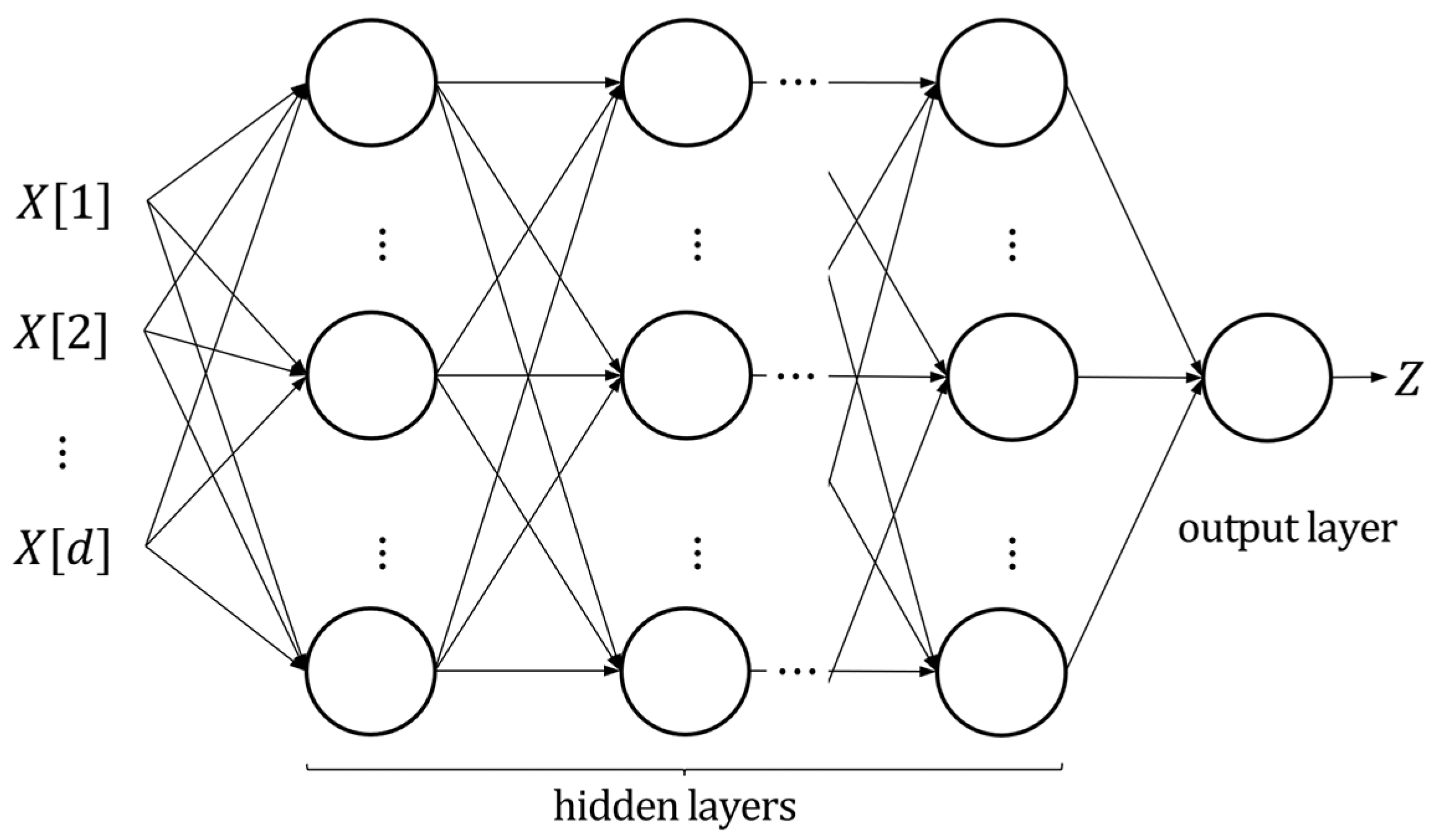
First, we explain the configuration of an MLP to express a general multi-dimensional function and to approximate the continuation value function in the multi-dimensional Bermudan option problem.

The basic configuration of the MLP is shown in Figure 1, where $X\in {ℝ}^d$ is an input vector and $Z\in ℝ$ is an output of the entire neural network. Each neuron is called a “perceptron” that defines a mapping of input/output signals with appropriate dimensions, being dependent on the number of neurons at input/output layers. For example, if $\mathit{x}\in {ℝ}^{d_x}$ denotes an input signal of a perceptron with a weight matrix $\mathit{W}\in {ℝ}^{d_x\times d_y}$ and a bias vector $\mathit{b}\in {ℝ}^{d_y}$, then, an output signal $\mathit{y}\in {ℝ}^{d_y}$ from the perceptron is given by

$$\mathit{y}=h\left({\mathit{W}}^T\mathit{x}+\mathit{b}\right),$$

(6)

where $h: {ℝ}^{d_y}\to {ℝ}^{d_y}$ is a component-wise activation function. Typical choices of activation functions in neurons are as follows:

$$\begin{array}{c}\mathrm{Sigmoid}: x\mapsto \frac{1}{1+e^{-x}}\\ \mathrm{ReLU}:x\mapsto \max \left(x, 0\right) \end{array}.$$

(7)

In the case where the MLP is applied for a regression, all the weight matrices and bias vectors in the MLP are computed to minimize the sum of squared errors between the actual dependent variable, denoted by $Z\in ℝ$, and the predicted dependent variable $\widehat{Z}\in ℝ$ given the training datasets of $X\in {ℝ}^{d_x}$ and $Z\in ℝ$ (expressed using the MLP in Figure 1).

Note that the MLP can express a continuous and complex nonlinear surface in entire networks by sequentially performing a linear and nonlinear transformation on inputs $X\in {ℝ}^{d_x}$ to the compiled layer output $\widehat{Z}\in ℝ$. The properties of the MLP function derive from the universal approximation theorem proposed by Cybenko (1989) and the Kolmogorov–Arnold representation theorem put forward by Kolmogorov (1957) and Arnold (2009), in which any function can be approximated if the input size and network are infinite. In this sense, functions expressed by the MLP are generally considered suitable for a problem with complicated interactions because of the adjustable basis functions (see Choon et al. 2008).

For the randomly generated sample paths of ${\left(X_t\right)}_{0\le t\le T}$, we can apply the LSMC method (see Appendix A and Appendix B) combined with the MLP, whereby the continuation value function is modeled at each step using a function given by the MLP. Let $X_t^{\left(1\right)},X_t^{\left(2\right)},\dots ,X_t^{\left(M\right)}$ and $0\le t\le T$ be the simulated $M$ sample paths of ${\left(X_t\right)}_{0\le t\le T}$. Since the discrete-time payoff process $P_{T_n}$ (if exercised at times ${\left(T_n\right)}_{0\le n\le N}$) is specified as a function of $X_{T_n}$ for a Bermudan option and $Z_{T_N}=P_{T_N}$, the training data of the output variable, $Z\equiv Z_{T_N}\in ℝ$, in the first step of the LSMC method, are computed as $P_{T_N}^{\left(1\right)},P_{T_N}^{\left(2\right)},\dots ,P_{T_N}^{\left(M\right)}$, corresponding to the payoffs of the Bermudan option at maturity along the sample path of $X_{T_N}$. The MLP in the first step is constructed for the training data of $X\equiv X_{T_{N-1}}\in {ℝ}^{d_x}$, given as $X_{T_{N-1}}^{\left(1\right)},X_{T_{N-1}}^{\left(2\right)},\dots ,X_{T_{N-1}}^{\left(M\right)}$, together with those of $Z\equiv Z_{T_N}\in ℝ$. Then, we obtain an approximation of the continuation value function, denoted by ${\widehat{\Phi }}_{N-1}$, and the continuation values along the sample path, ${\widehat{\Phi }}_{N-1}\left(X_{T_{N-1}}^{\left(m\right)}\right), m=1,\dots ,M.$

In the second step, the training data of the output variable, $Z\equiv Z_{T_{N-1}}\in ℝ$, are computed using (1), as

$$Z_{T_{N-1}}^{\left(m\right)}=max\left(P_{T_{N-1}}^{\left(m\right)}, {\widehat{\Phi }}_{N-1}\left(X_{T_{N-1}}^{\left(m\right)}\right)\right), m=1,\dots , M,$$

(8)

as well as the training data of $X\equiv X_{T_{N-2}}\in {ℝ}^{d_x}$, given as $X_{T_{N-2}}^{\left(1\right)},X_{T_{N-2}}^{\left(2\right)},\dots ,X_{T_{N-2}}^{\left(M\right)}$. Using these training datasets, the MLP is constructed to find an approximation of the continuation value function, denoted by ${\widehat{\Phi }}_{N-2}$, and the continuation values along the sample paths, ${\widehat{\Phi }}_{N-2}\left(X_{T_{N-2}}^{\left(m\right)}\right).$ We then repeat the same procedure until $T_0.$

3.2. Learning Networks and Option Pricing

For learning neural networks, we generate Monte Carlo sample paths using the SDEs in Section 3.2 based on a similar idea to that of the ordinary LSMC method introduced by Longstaff and Schwartz (2001). Herein, we apply nonlinear functions of the MLPs instead of polynomial functions for the basis of the continuation value functions. Additionally, we introduce techniques such as early stopping to improve the fitted continuation functions and avoid possible overfitting or biases in learning and pricing. We also introduce the resampling procedure to avoid a possible bias caused by using the same random samples between learning and valuation, and we regenerate Monte Carlo sample paths for the valuation of Bermudan option prices (see Appendix A for pricing details).

Herein, we summarize a learning procedure, as described in Algorithm 1 below, where the underlying price and the volatility vector are denoted by $S_t:={\left[S_{1,t},S_{2,t},\dots ,S_{l,t}\right]}^{\top }$ and ${\sigma }_t:={\left[{\sigma }_{1,t},{\sigma }_{2,t}, \dots ,{\sigma }_{l,t}\right]}^{\top }$, while $g$ denotes a payoff function of $S_t$. Given simulation the sample paths generated by the multi-asset stochastic volatility models in (4), we provide a Bermudan option pricing procedure involving the algorithm for estimating the continuation values using neural networks. This algorithm operates to find MLP $\Phi$ as a continuation value function satisfying Equation (8) in the previous section and gives the Bermudan option price.

Algorithm 1. Bermudan option pricing with learning networks.

Require: Initiate paths $S_t^{\left(j\right)}$, ${\mathsf{\sigma }}_t^{\left(j\right)}$, $t=T_0,T_1,\cdots ,T_N$, $j=1,2,\cdots ,M$

1:Let $p$ be the patience and $Ma{x}_{iter}$ be the maximum number of epochs

2:Put $V^{\left(j\right)}\leftarrow g\left(S_{T_N}^{\left(j\right)}\right)$ for all $j$

3:for $t$ from $T_{N-1}$ to $T_1$ do

4: Let $X^{\left(j\right)}\leftarrow S_t^{\left(j\right)},{\mathsf{\sigma }}_t^{\left(j\right)}$ and $V^{\left(j\right)}\leftarrow e^{-r\mathsf{\delta }t}\cdot V^{\left(j\right)}$ for all $j$

5: if $t$ on exercisable periods then

6:  Perform learning on $X$ to obtain network ${\Phi }_t$ with $Z$ to be $V$

7:  $i\leftarrow 0$

8:  $k\leftarrow 0$

9:  while $i<Ma{x}_{iter}$ do

10:   Train ${\Phi }_t$ on $X$ and $V$

11:   if improved then

12:    $k\leftarrow 0$

13:   else

14:    $k\leftarrow k+1$

15:   end if

16:   if $k==p$ then

17:    Break

18:   end if

19:   $i\leftarrow i+1$

20:  end while

21:  Calculate the continuation value ${\Phi }_t\left(X^{\left(j\right)}\right)$ for all $j$

22:  for $j$ from $1$ to $M$ do

23:   if $g\left(S_t^{\left(j\right)}\right)>{\Phi }_t\left(X^{\left(j\right)}\right)$ then

24:    $V^{\left(j\right)}\leftarrow g\left(S_t^{\left(j\right)}\right)$

25:   end if

26:  end for

27: end if

28:end for

29:return mean of $e^{-r\mathsf{\delta }t}\cdot V$

Note This study does not use the selection technique, which performs regression using only the in-the-money paths proposed by Longstaff and Schwartz (2001), for the purpose of constructing a versatile algorithm.

It is noted that one cycle of training with the complete training data is known as an epoch and is repeated for learning purposes for each continuation value function in Algorithm 1. In general, the larger the number of epochs, the better learning of the training data. However, a large number of epochs usually requires a long computational time, even with large computer resources, and sometimes leads to overfitting of the training data. To prevent such situations, we introduce an early stopping rule for the learning procedure given a specified integer $p$ in Algorithm 1. Under the early stopping rule, the objective function (3) is monitored for improvement, and the number of iterations (i.e., the number of epochs) without improvement (compared with the previous epoch), denoted by $k$, are counted. If this number reaches $p$, the iteration stops and the learning procedure of the continuation value function terminates; otherwise, the iteration continues as long as the iteration index $i$ is less than $Ma{x}_{iter}$, where $Ma{x}_{iter}$ is the maximum number of epochs specified at the beginning of Algorithm 1. Note that the introduction of the early stopping rule not only decreases the computational time but also prevents overfitting/underfitting for the MLP.

Based on the network configuration of the neural networks, the computational complexity of Algorithm 1 is given by the number of iterations for parameter estimation of the MLP. This number of iterations depends on the maximum number of epochs and the number of exercisable dates, $Ma{x}_{iter}$ and $N-1$. Once these values are specified, the maximum number of iterations is $Ma{x}_{iter}\times \left(N-1\right)$, which is the total number of epochs applied in Algorithm 1. In addition, the computational complexity of each epoch in the MLP depends on the network configuration (see Serpen and Gao 2014).

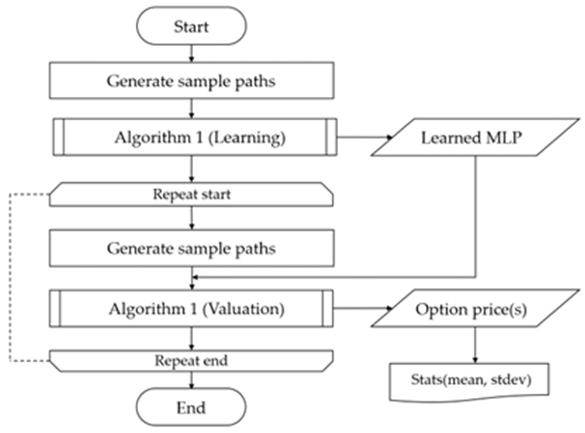
To price the Bermudan commodity options using the continuation functions estimated in Algorithm 1, we regenerate different sample paths from those used in the learning procedure for computing the continuation values and Bermudan commodity option prices, given the neural networks in Algorithm 1, i.e., we separate the learning and the valuation procedures, and Algorithm 1 may be applied without learning (i.e., given the estimated neural networks) for the valuation procedure. The merit of this resampling is that it avoids a price bias, which results from overfitting using the same sample paths. Accordingly, this study adopts the following procedure:

• Generate the sample paths of the underlying assets for the MLP learning of Algorithm 1.
• Find the MLP network parameters via learning in Algorithm 1 using the sample paths in Step 1.
• Given the estimated neural networks, regenerate a different set of sample paths and apply Algorithm 1 (without learning) to compute the continuation values and the initial prices of the Bermudan options.
• Repeat Step 2 and calculate statistical values such as the mean and the standard deviation of the Bermudan option prices.

In the above, it is key that learning and pricing (i.e., valuation) utilize the different simulation sample paths set in Steps 1 and 3. Figure 2 shows a flowchart of the entire procedure for learning and valuation.

4. Numerical Experiments

The objective of this section is to execute numerical experiments based on the learning and valuation procedure explained in the previous section and make comparisons of the Bermudan option pricing between the MLP and the benchmark polynomial regression (i.e., the standard (naïve) LSMC method by Longstaff and Schwartz 2001).

4.1. Problem Setting and Preliminary Experiment

Herein, we consider Bermudan commodity options with early-exercisable dates in discretized periods until maturity $T$, i.e., $0=T_0<T_1<\dots <T_N=T$, the payoffs of which are given by $g\left(S_t\right)$ when exercised. We define several settings for different dimensions of Bermudan options, $d_l$ (i.e., the number of state variables in (5)), exercisable dates, and payoff functions. We also introduce a constant volatility model as a one-dimensional problem to perform a preliminary experiment.

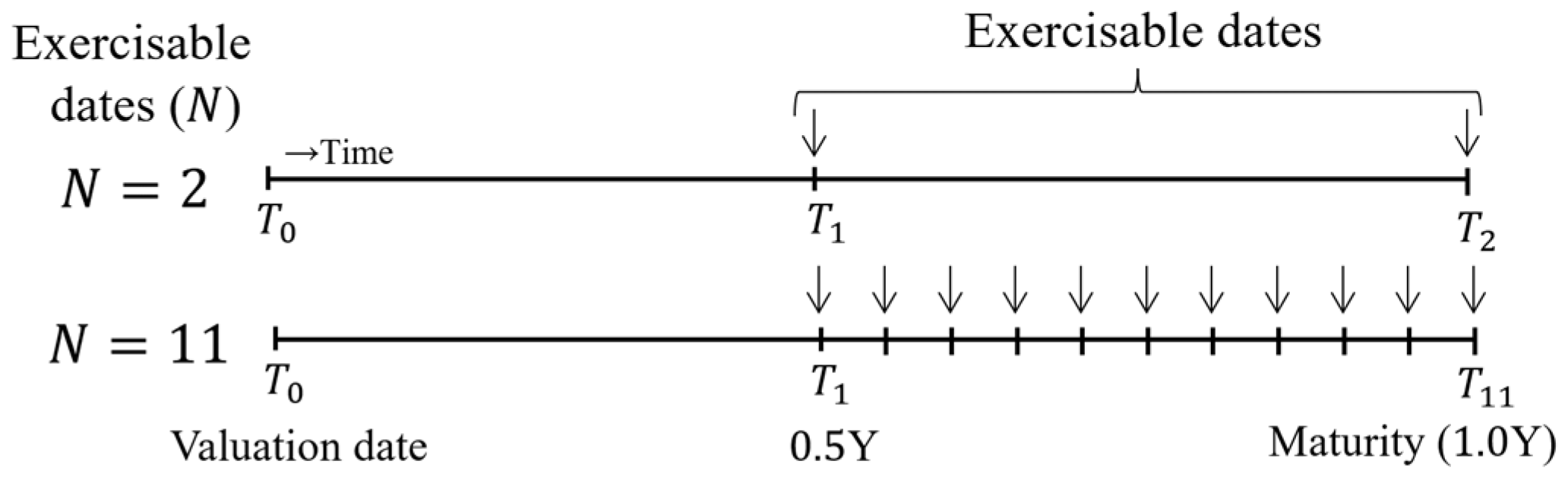
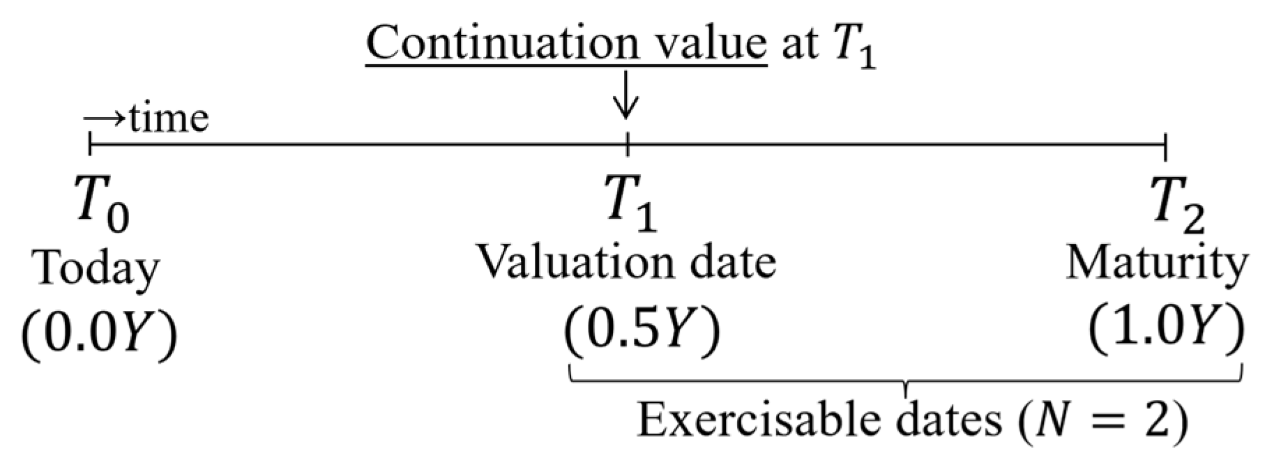
For the exercisable dates of the Bermudan commodity options, we consider two cases as depicted in Figure 3. One is a two-period problem, wherein the Bermudan commodity option is issued at time $T_0$ and can be exercised at $T_1$ and maturity $T_2.$ The other is a case with multiple exercisable dates, wherein we choose ten exercisable timings before maturity. In both cases, the options can be exercised after a half-year period to compare the continuation value surfaces at time $T_1$ between different methodologies, and the values of the options are evaluated at the initial time period, $T_0$.

Moreover, the payoff functions for Bermudan basket put options are given as

$$g\left(S_t\right)=\max \left(K-\frac{1}{l}{\displaystyle \sum }_i{S}_{i,t},0\right).$$

(9)

Then, an upper limit price $D$ is introduced to the payoff function as

$$g\left(S_t\right)=\min \left(\max \left(K-\frac{1}{l}{\displaystyle \sum }_i{S}_{i,t},0\right),D\right)$$

(10)

for Bermudan capped put options. Note that the upper limit, $D$, provides an additional complexity of the payoff functions.

The parameters of the underlying assets and neural networks are set as shown in

Table 1. Parameters of the underlying asset model with constant and stochastic volatility.

Parameter	$\mathbf{Constant} \mathbf{Vol}. ({\mathit{d}}_{\mathit{l}}=1)$	$\mathbf{Stochastic} \mathbf{Vol}. ({\mathit{d}}_{\mathit{l}}\ge 2){ }^1$
Spot rate ($S_0$)	100.0
Strike rate ($K$)	105.0
Capped rate ($D$)	10.0
Time to maturity ($T$) [years]	1.0
Risk-free interest rate ($r$) [%]	6.0
Initial volatility (${\sigma }_{i,0}$) [%]	30.0
Long-run mean ($\mu$)	4.8
Kappa of asset (${\kappa }_{S_i}$)	0.3
Long-term volatility ($\sqrt{{\vartheta }_i}$) [%]	-	30.0
Correlation (${\rho }_{S_i, v_i}$)	-	−0.1
Corr. among assets (${\rho }_{S_i, S_j}$)	-	0.7 (1.0 $if i=j$)
Corr. assets and vol. (${\rho }_{S_i, v_j}$)	-	−0.07
Corr. among vols. (${\rho }_{v_i, v_j}$)	-	0.007 (1.0 $if i=j$)
Kappa of vol. (${\kappa }_{v_i}$)	-	1.5
Vol. of vol. (${\xi }_i$)	-	0.2
Num. of paths (learning)	100,000
Num. of paths (valuation)	10,000
Sim. path timesteps (per yr.)	20

¹ We applied Euler’s method as a discretized method.

and

Table 2. Neural networks’ learning parameters.

Learning Parameters	Value
Num. of sim. paths ($M$)	100,000
Batch size	4096
Max. num. of epochs ($Ma{x}_{iter}$)	200
Train paths percentage	80%
Evaluation paths percentage	20%
Optimizer	Adam 1

¹ Learning optimizer Adam (Kingma and Ba 2014) hyperparameters are set to 0.01 for the learning rate, $0.9$ for beta1, 0.999 for beta2, and 1 × 10⁻⁷ for epsilon; training is completed when the loss does not improve even after 20 epochs, as early stopping. Randomized 20% of input paths are used in evaluations to avoid over-learning.

below.

4.2. Low-Dimensional Case: Single-Asset Bermudan Options with Stochastic Volatility and Constant Volatility

We begin with the simplest valuation based on Schwartz’s (1997) single-asset and constant volatility model in, compared with the standard LSMC method using polynomial regression and the finite difference method (FDM) detailed by Tavella and Randall (2000). In the MLP, we applied Algorithm 1 for learning neural networks with Monte Carlo simulations and then repeated the valuation procedure (using Algorithm 1 without learning) 100 times. The MLP in this experiment contains two hidden layers with sixty-four neurons of sigmoid activate functions. In the standard LSMC method, we use a quintic function for one-dimensional problems (i.e., $d_l=1$) and a multi-dimensional quadratic function for two or more higher-dimensional problems (i.e., $d_l\ge 2$) and apply the same procedure (i.e., the learning and valuation procedure). The FDM is based on the Crank–Nicolson scheme with discretized 2000/200/50 grids in the time/asset/volatility directions.

Table 3. Bermudan (capped) put option prices in single-asset constant volatility ($d_l=1$).

$\mathbf{Bermudan} \mathbf{Put} \mathbf{Option} ({\mathit{d}}_{\mathit{n}}=1)$				$\mathbf{Bermudan} \mathbf{Capped} \mathbf{Put} \mathbf{Option} ({\mathit{d}}_{\mathit{n}}=1)$
	# of Ex.	N = 2	N = 11		# of Ex.	N = 2	N = 11
LSMC price	Mean	11.474	11.786	LSMC price	Mean	5.731	6.244
	(St. dev.)	(0.071)	(0.069)		(St. dev.)	(0.027)	(0.029)
MLP price	Mean	11.471	11.812	MLP price	Mean	5.729	6.320
	(St. dev.)	(0.069)	(0.061)		(St. dev.)	(0.027)	(0.031)
FDM price		11.415	11.808	FDM price		5.752	6.350

^note FDM = finite difference method; LSMC = least-squares Monte Carlo; MLP = multi-layer perceptron.

compares the means and standard deviations of the option prices obtained with the MLP and the standard LSMC methods. Considering the option price of the FDM as a proxy for the value of the Bermudan commodity option price, we see that both the MLP and the standard LSMC method almost achieve the Bermudan option price value, i.e., the gap between the three prices is sufficiently small for this one-dimensional problem. We implemented Algorithm 1 using the MLP and the standard LSMC on Python, using a machine learning package based on TensorFlow (Abadi et al. 2015) and the PolynomialFeatures toolbox of the scikit-learn library (Pedregosa et al. 2011). All our numerical experiments were run using Google Colaboratory (Google 2022) with 36 GB of RAM and a dual-core CPU of 2.3 GHz.

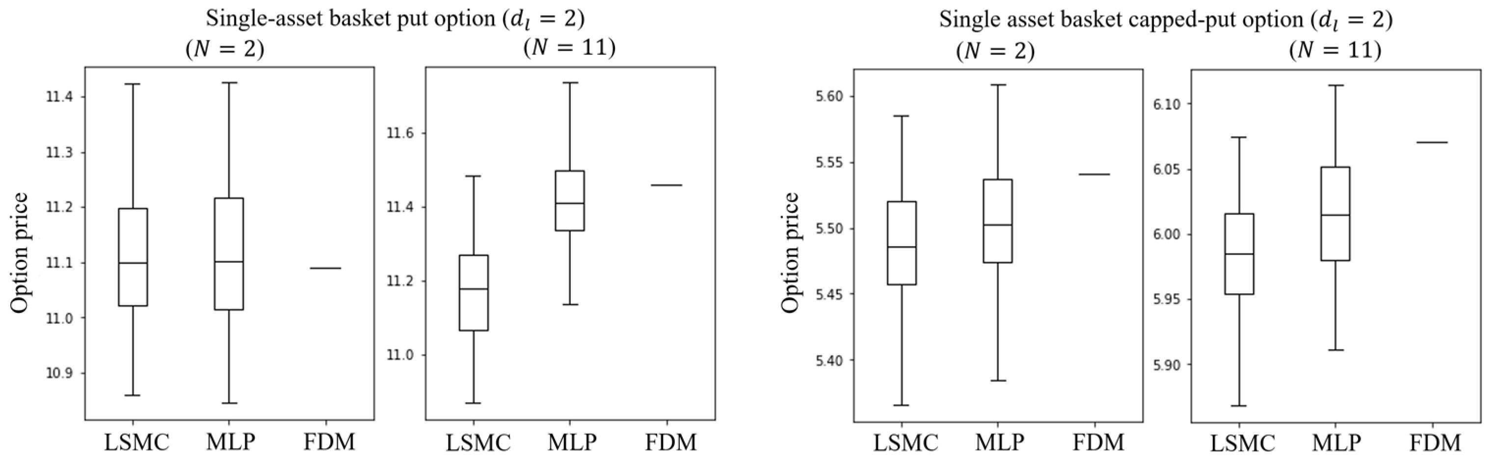
When considering a single-asset stochastic model, the corresponding Bermudan commodity option problem becomes two-dimensional, i.e., $d_l=2$, we can observe a slight difference between the MLP and the LSMC methods, compared with the approximate solution of the FDM, as shown in

Table 4. Bermudan (capped) put option prices in single-asset stochastic volatility ($d_l=2$).

$\mathbf{Bermudan} \mathbf{Put} \mathbf{Option} ({\mathit{d}}_{\mathit{l}}=2)$				$\mathbf{Bermudan} \mathbf{Capped} \mathbf{Put} \mathbf{Option} ({\mathit{d}}_{\mathit{l}}=2)$
	# of Ex.	N = 2	N = 11		# of Ex.	N = 2	N = 11
LSMC price	Mean	11.114	11.170	LSMC price	Mean	5.489	5.985
	(St. dev.)	(0.139)	(0.137)		(St. dev.)	(0.047)	(0.043)
MLP price	Mean	11.113	11.417	MLP price	Mean	5.504	6.015
	(St. dev.)	(0.140)	(0.133)		(St. dev.)	(0.047)	(0.045)
FDM price		11.090	11.460	FDM price		5.541	6.070

. First, we see that there is no significant difference between the 3 cases for the Bermudan put option with exercisable dates $N=2$. However, the gap between the LSMC and FDM prices becomes slightly wider, compared with that between the MLP and FDM prices with exercisable dates $N=11$. For the Bermudan capped put option, there is a slightly larger difference vis-à-vis the FDM price for both the MLP and LSMC prices, whereas a slight improvement was achieved by using the MLP in terms of the gap from the FDM price, as illustrated in the box plots in Figure 4.

4.3. Higher-Dimensional Case: Multi-Asset Bermudan Options with Stochastic Volatility

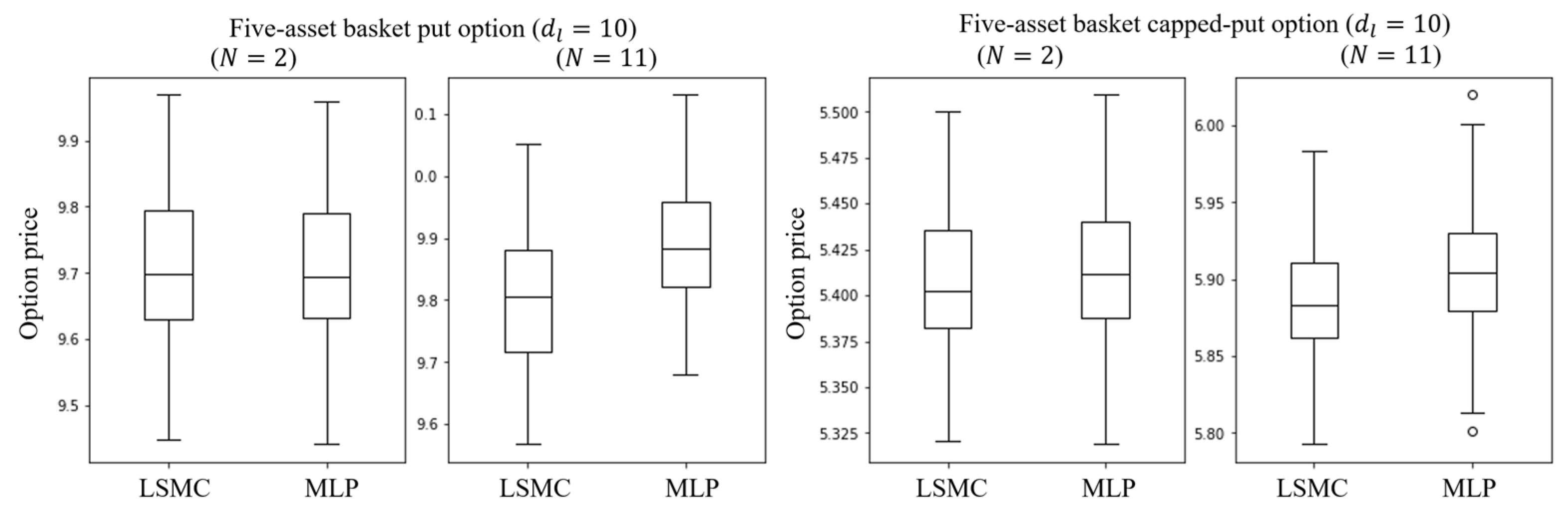
In the case of higher-dimensional Bermudan commodity options with multi-asset stochastic volatility (e.g., two asset problems with $d_l=4$), it is difficult (or unrealistic) to obtain an approximate Bermudan option price with high accuracy using the FDM. Thus, we compare option prices obtained with the MLP with the benchmark polynomials (i.e., the standard LSMC method) only, where we set $d_l=10$, i.e., five-asset stochastic volatility, in the numerical experiments. Then, we will discuss the source of the difference in view of the continuation value functions for both methods in the next section. Additionally, we will compare the accuracy of estimated continuation values by considering a two-asset problem with $d_l=4$ and two exercisable dates $N=2$.

Table 5. Bermudan (capped) put option prices in the five-asset ($d_l=10$) stochastic volatility model.

$\mathbf{Bermudan} \mathbf{Put} \mathbf{Option} ({\mathit{d}}_{\mathit{l}}=10)$				$\mathbf{Bermudan} \mathbf{Capped} \mathbf{Put} \mathbf{Option} ({\mathit{d}}_{\mathit{l}}=10)$
	# of Ex.	N = 2	N = 11		# of Ex.	N = 2	N = 11
LSMC price	Mean	9.712	9.803	LSMC price	Mean	5.406	5.884
	(St. dev.)	(0.108)	(0.105)		(St. dev.)	(0.043)	(0.039)
MLP price	Mean	9.712	9.888	MLP price	Mean	5.414	5.904
	(St. dev.)	(0.103)	(0.098)		(St. dev.)	(0.043)	(0.040)

shows our numerical results, which compare the mean and standard deviation between the LSMC and the MLP prices for $N=2$ and $N=11$, obtained via the learning and valuation procedure described in Section 3. In the case of the Bermudan put option for $N=2$, we see that there is no significant difference between the two methods, as with the case with a low-dimensional problem, $d_l=2$. However, the gap between the two increased for the Bermudan capped put options and the case with $N=11$, as shown in the box plots in Figure 5. In other words, we see that the differences between the MLP and the LSMC are emphasized by introducing additional complexity to the payoff function or by increasing exercisable dates.

Additionally, we demonstrated the same numerical experiments above but increased the number of assets in the stochastic volatility model to 10 and 20 assets, respectively (i.e., $d_l=20$ and $d_l=40$) and compared the estimated Bermudan commodity option prices between the MLP and the LSMC. To observe the effects of increasing the number of exercisable dates more clearly, we added $N=6$ between $N=2$ and $N=11$ to obtain the estimation values shown in

Table 6. Bermudan (capped) put option prices in the 10-asset ($d_l=20$) stochastic volatility model.

$\mathbf{Bermudan} \mathbf{Put} \mathbf{Option} ({\mathit{d}}_{\mathit{l}}=20)$					$\mathbf{Bermudan} \mathbf{Capped} \mathbf{Put} \mathbf{Option} ({\mathit{d}}_{\mathit{l}}=20)$
	# of Ex.	N = 2	N = 6	N = 11		# of Ex.	N = 2	N = 6	N = 11
LSMC price	Mean	9.539	9.595	9.571	LSMC price	Mean	5.359	5.747	5.848
	(St. dev.)	(0.120)	(0.098)	(0.097)		(St. dev.)	(0.036)	(0.042)	(0.041)
MLP price	Mean	9.548	9.681	9.684	MLP price	mean	5.376	5.765	5.851
	(St. dev.)	(0.112)	(0.091)	(0.095)		(St. dev.)	(0.035)	(0.041)	(0.041)
Difference (MLP—LSMC)	Mean	0.009	0.087	0.113	Difference (MLP—LSMC)	Mean	0.016	0.018	0.003

and

Table 7. Bermudan (capped) put option prices in the 20-asset ($d_l=40$) stochastic volatility model.

$\mathbf{Bermudan} \mathbf{Put} \mathbf{Option} ({\mathit{d}}_{\mathit{l}}=40)$					$\mathbf{Bermudan} \mathbf{Capped} \mathbf{Put} \mathbf{Option} ({\mathit{d}}_{\mathit{l}}=40)$
	# of Ex.	N = 2	N = 6	N = 11		# of Ex.	N = 2	N = 6	N = 11
LSMC price	Mean	9.338	9.4855	9.453	LSMC price	Mean	5.362	5.728	5.828
	(St. dev.)	(0.112)	(0.111)	(0.111)		(St. dev.)	(0.048)	(0.042)	(0.037)
MLP price	Mean	9.369	9.596	9.600	MLP price	Mean	5.382	5.750	5.833
	(St. dev.)	(0.111)	(0.105)	(0.104)		(St. dev.)	(0.048)	(0.040)	(0.037)
Difference (MLP—LSMC)	Mean	0.031	0.111	0.147	Difference (MLP—LSMC)	Mean	0.020	0.022	0.005

(corresponding to the cases of $d_l=20$ and $d_l=40$, respectively). Table 6 shows the means, the standard deviations, and the gaps between the estimated prices for the Bermudan put options and Bermudan capped put options with $d_l=20$, and Table 7 shows those with $d_l=40$.

Similar to the previous cases, the gap between the MLP and LMSC increases for the Bermudan put prices given a larger number of exercisable dates but decreases for the Bermudan capped put options when $N=11$ for both $d_l=20$ and $d_l=40$. It is possible that the choice of regression function has a weaker effect for higher dimensional Bermudan capped put options with a larger number of exercisable dates, i.e., the continuation value functions of the capped put options may become flatter or smoother when the number of exercisable dates increases and can be fitted with less sophisticated functions. This phenomenon should be investigated in more detail in a future study.

4.4. Comparison of Continuation Value Surfaces

In the previous subsection, we observed that there are some differences between the MLP and the LSMC regarding the estimated prices and that these differences were more notable for Bermudan capped put options and/or increased exercisable dates. Herein, we discuss the possible reason for this price difference by visualizing the continuation value surfaces for both the MLP and the LSMC methods. For visualization purposes, we consider single-asset Bermudan capped put options with stochastic volatility and constant volatility, i.e., the low-dimensional cases with $d_l=1$ and $d_l=2$ introduced in Section 4.2.

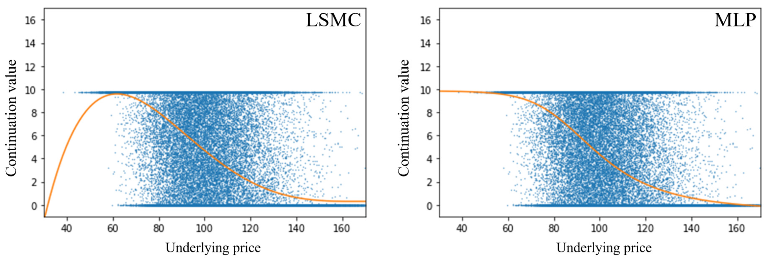
The left-hand plot of Figure 6 illustrates the continuation value function estimated at $T_1$ in the one-dimensional Bermudan capped-put option problem (corresponding to the single-asset constant volatility model) using the LSMC, whereas the right-hand plot shows the problem using the MLP. We first observe that the continuation value function of the MLP monotonically decreases with the underlying price, whereas the one obtained from the LSMC method is a nonmonotonic function. Since the payoff function of the Bermudan capped put option is piecewise linear and it monotonically decreases with the underlying price, the monotonicity of the continuation value function is more consistent with the payoff structure of the Bermudan capped-put option. In this sense, we see that the continuation value function of the MLP reflects the monotonic property more appropriately than that of the LSMC method in the one-dimensional single-asset problem.

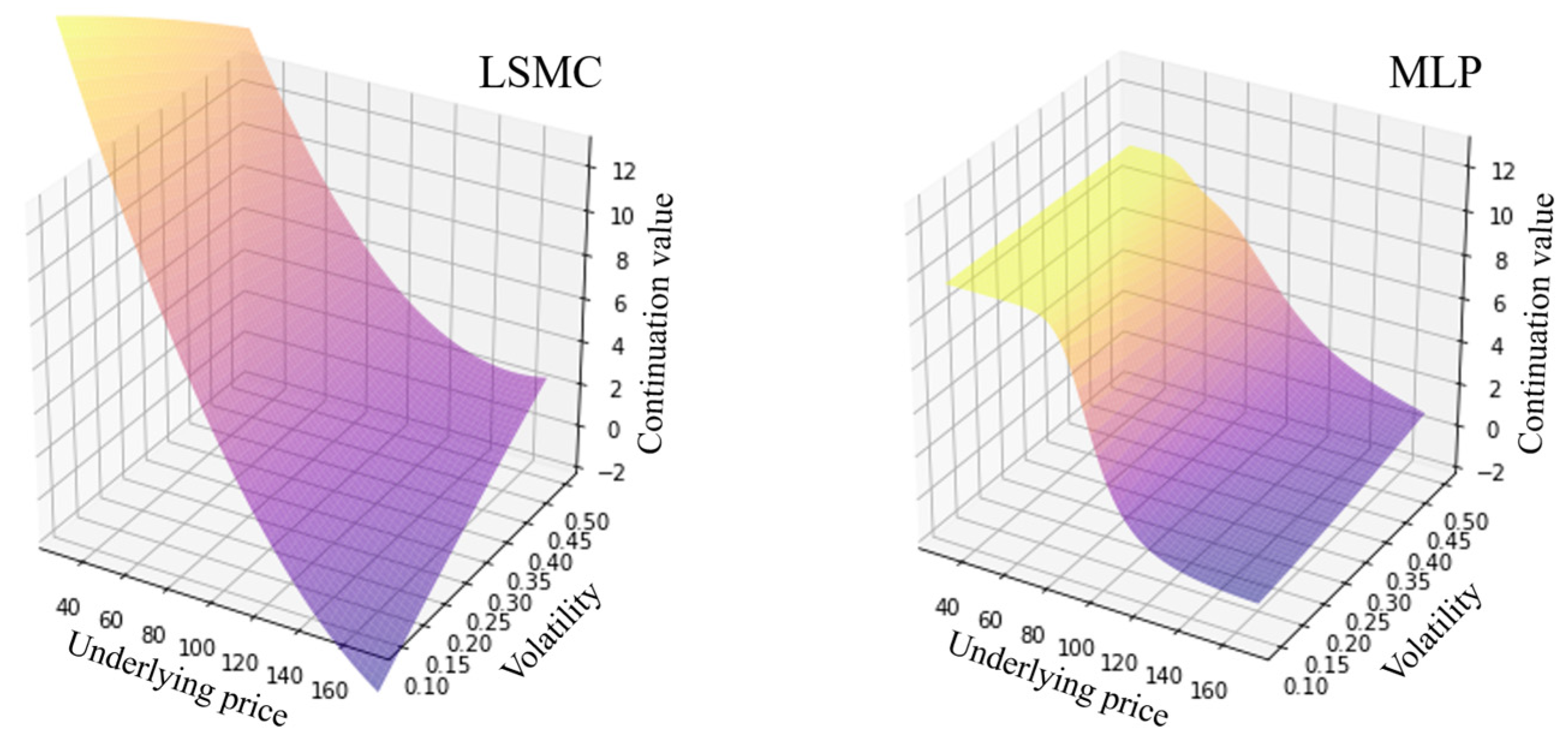
For the two-dimensional case with single-asset stochastic volatility for Bermudan capped put options, the continuation value functions have three-dimensional surfaces, as shown in Figure 7, wherein the left-hand and right-hand plots depict the continuation values with respect to volatility and underlying asset price directions for the LSMC method and the MLP, respectively. As in the one-dimensional problem, the payoff function is piecewise linear with respect to the underlying asset price direction and is flat when the underlying asset price exceeds the strike price $K=105$ or is less than a certain value related to the capped rate $D=10$. Since continuation value functions are supposed to approximate the payoff function at the maturity $T_2$, given the information up to time $T_1$, their surfaces are expected to have similar shapes, i.e., continuation values are approximately zero or close to the capped rate for larger or smaller values of the underlyings, respectively. In view of this payoff structure for the Bermudan capped put options, the continuation value surface of the MLP seems to approximate the payoff function more accurately than that of the LSMC.

Remark 1. 

In general, the visualization of nonparametric methods provides an intuitive interpretation of the estimated functions. We have observed that “the continuation value function of the MLP monotonically decreases with the underlying price, whereas the one obtained from the LSMC method is a non-monotonic function,” and that “since the payoff function of the Bermudan capped-put option is piecewise linear and it monotonically decreases with the underlying price, the monotonicity of the continuation value function is more consistent with the payoff structure of the Bermudan capped-put option,” as stated earlier in this section. Such a visualization helps in understanding the valuation structure for the applied method in the middle of the process for Bermudan option pricing, but the effect of the approximation error may be weakened in the total procedure. However, we should be able to understand the approximation errors of estimated continuation value functions intuitively in the middle of the process from such a visualization.

4.5. Comparison of Accuracy in Continuation Values

In the previous subsection, we observed that the continuation value surfaces of the MLP may approximate the payoff functions more accurately than those of the LSMC by visualizing the continuation value surfaces. To further investigate the estimated continuation value surfaces in higher-dimension problems, we next measure the accuracy of the continuation values using a four-dimensional problem of the Bermudan capped put basket option with two exercisable dates (i.e., $d_l=4$ and $N=2$) for both the MLP and the LSMC method.

Consider a problem of estimating the continuation values at $T_1$, as shown in Figure 8. Since Bermudan options with exercisable dates $N=2$ become simple European options if not exercised at $T_1$, the continuation values at $T_1$ may be estimated via European option prices expiring at $T_2$, given the state variables at $T_1$, i.e., $X_{T_1}={\left[S_{1,T_1},{\sigma }_{1,T_1}, S_{2,T_1},{\sigma }_{2,T_2}\right]}^{\top }$. Therefore, we can calculate the accuracy of the estimated continuation values at $T_1$ by measuring the differences between the estimated continuation values and the European option prices at $T_1$ by specifying different state variables as input values of the European options.

We first solved the Bermudan option problem with $d_l=4$ and $N=2$ using the same parameter settings as those in the previous subsections by applying the MLP and the LSMC methods; subsequently, we calculated the continuation values at $T_1$, given the state variables specified in

Table 8. State variables at $T_1$. Each state variable is equally discretized into the number of points from minimum up to maximum value.

Variable	Minimum	Maximum	# of Points 1	Interval
$S_{1,T_1}$	25.0	175.0	$2^4+1$	9.375
${\sigma }_{1,T_1}$	0.05	0.55	$2^4+1$	0.03125
$S_{2,T_1}$	25.0	175.0	$2^4+1$	9.375
${\sigma }_{2,T_1}$	0.05	0.55	$2^4+1$	0.03125

¹ The number of grid points with state variables at $T_1$ are 83,521 ($={17}^4$) in total. The number of sample paths generated for evaluating each European option in the standard Monte Carlo simulation is 10,000. The average values of estimated European prices and standard errors are $4.997$ and $0.027$, respectively, indicating that the 95% confidence interval is given by $4.997\pm 0.053$ on average for the Monte Carlo simulations.

. Note that Table 8 defines the discretized domain of the state variables, wherein each state variable is discretized in the interval between the minimum and maximum values so that the number of grid points in 1 dimension becomes $2^4+1$. Then, the total number of grid points is given by 83,521 ($={17}^4$). Similarly, we applied the standard Monte Carlo simulation to compute the European option price on each grid and repeated this procedure 83,521 times to estimate the surface of the European option prices. This surface of the European option prices may be considered to provide an approximation of the theoretical continuation value (see notes in Table 8), and we can measure the accuracy of the continuation values using the difference between the estimated continuation values with the MLP and the LSMC methods and the simulation-based (theoretical) surface.

Additionally, we can change the number of hidden layers/neurons and the type of activation function in the MLP to verify their effects on its accuracy. In this study, we evaluate the size of accuracy in terms of the following normalized root-mean-squared error (NRMSE) for each methodology:

$$NRMSE=\frac{1}{\sqrt{I}}\frac{\sqrt{{{\displaystyle \sum }}_{i=1}^I{\left(p_i-\widehat{p_i}\right)}^2}}{{\widehat{p}}_{max}-{\widehat{p}}_{min}},$$

(11)

where $I$ is the total number of grid points (i.e., $I=\mathrm{83,521}$), and $p_i$ and $\widehat{p_i}$ are the $i^{th}$-continuation value and the corresponding European option price on the same grid point. In Equation (11), the root-mean-squared error is normalized by the difference between ${\widehat{p}}_{min}$ and ${\widehat{p}}_{max}$, which are the minimum and maximum values of European option prices over the entire grid.

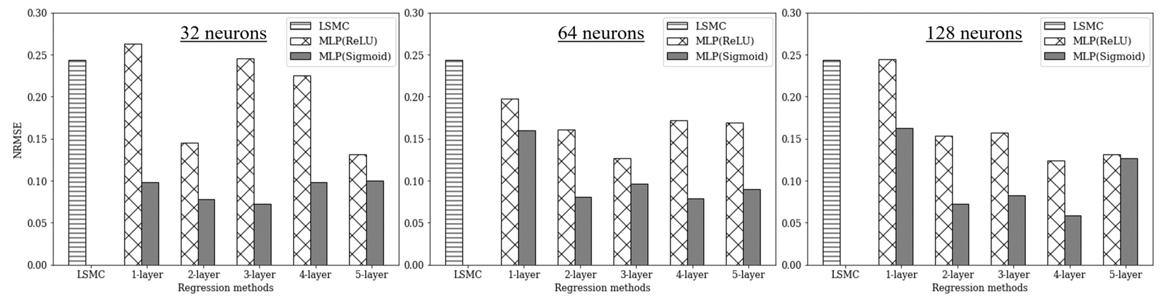
We computed the NRMSEs for different settings of neural networks in the case of the MLP, as shown in

Table 9. NRMSE comparisons with continuation values at $T_1$ by network settings of the MLP. It differs by activation functions and the number of hidden layers/neurons.

NRMSE
# of Neurons	16		32		64		128		256
# of Hidden Layers	ReLU	Sigmoid	ReLU	Sigmoid	ReLU	Sigmoid	ReLU	Sigmoid	ReLU	Sigmoid
1	0.266	0.075	0.262	0.099	0.198	0.160	0.244	0.162	0.160	0.211
2	0.176	0.101	0.145	0.078	0.161	0.081	0.154	0.073	0.311	0.100
3	0.215	0.083	0.246	0.072	0.126	0.097	0.157	0.083	0.271	0.085
4	0.128	0.115	0.225	0.098	0.172	0.079	0.124	0.059	0.184	0.082
5	0.137	0.097	0.132	0.100	0.169	0.090	0.132	0.127	0.154	0.076
LSMC	0.244

^note NRMSE = normalized root-mean-squared error.

, wherein we changed the number of hidden layers/neurons and applied two types of activation functions, i.e., the ReLU and sigmoid functions. Note that the NRMSE with the LSMC method is also computed, as shown in the bottom row of the table, while Figure 9 compares the same NRMSE with respect to a different number of neurons for $16, 32,$ and $128$ using bar graphs. In Table 9, we first observe that the MLP almost always provided better accuracy in terms of NRMSEs compared with the LSMC. Second, when comparing the types of activation functions, the MLP with the sigmoid function was always better than the MLP with the ReLU function for estimating continuation value surfaces when the number of hidden layers/neurons was fixed. This may be explained by the smoothness of the sigmoid function; the continuation value functions are expected to be smooth with respect to the state variables and can be fitted via smooth functions (e.g., the sigmoid function) better than non-smooth functions, such as the ReLU function. Third, an increase in the number of hidden layers is effective for a few hidden layers but does not necessarily improve the NRMSE when the number of hidden layers is three or larger for both MLPs with the ReLU and sigmoid functions. However, in any case, we obtained better NRMSEs by using the MLP with the sigmoid function.

5. Discussion of Robustness and Computational Costs

In this section, we discuss the robustness and computational costs of our experiment for the pricing algorithm of multi-asset Bermudan commodity options using the MLP.

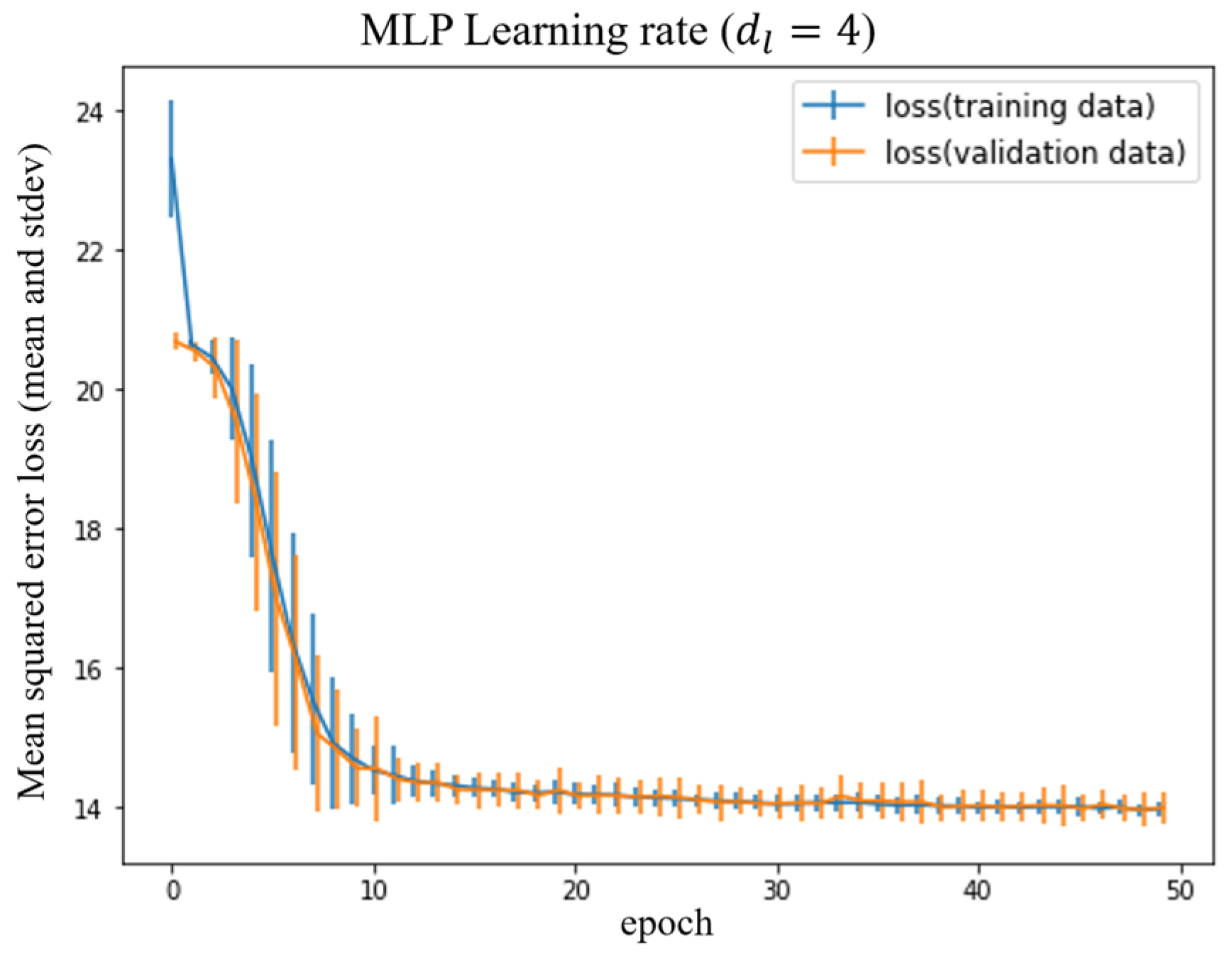
First, we discuss the learning adaptability of the MLP applied to our multi-asset Bermudan commodity option problems with stochastic volatility. Figure 10 depicts changes in the mean and standard deviation of learning rates with respect to the number of epochs in the MLP. In this figure, we see that training and validation losses remain close, which indicates no overfitting. Furthermore, the learning rate decreases rapidly until the number of epochs is 10 and stays at sufficiently good levels thereafter.

Next, we estimated the computational costs of the learning and valuation procedure when the problem dimension is increased.

Table 10. Computational cost comparisons. Each algorithm’s computational time periods (seconds) and their statistics by dimensions were calculated 100 times in the same option condition, as shown in Figure 10. In the MLP, the average numbers of epochs in learning are also listed.

	LSMC [Sec.]				MLP [Sec.] 2
Dimensions	Learning 1		Valuation		Learning			Valuation
$\left({\mathit{d}}_{\mathit{l}}\right)$	Mean	(St. Dev.)	Mean	(St. Dev.)	Mean	(St. Dev.)	# of Epochs	Mean	(St. Dev.)
2	0.025	(0.002)	0.003	(0.003)	20.038	(3.599)	186.19	0.006	(0.002)
4	0.076	(0.019)	0.003	(0.001)	17.637	(4.403)	156.56	0.006	(0.002)
8	0.257	(0.064)	0.005	(0.001)	17.382	(5.089)	157.43	0.006	(0.001)
16	0.861	(0.083)	0.020	(0.004)	9.773	(7.707)	81.99	0.007	(0.002)
32	3.708	(0.334)	0.068	(0.020)	5.114	(2.829)	38.53	0.008	(0.002)
64	19.887	(2.842)	0.210	(0.018)	5.367	(1.468)	36.58	0.009	(0.002)

¹ LSMC with a multi-dimensional quadratic function. ² MLP with 2 hidden layers with 64 neurons of sigmoid activation functions.

compares the computational costs with respect to the dimensions of $d_l=2, 4, 8, 16, 32, 64$, wherein the same numerical experiment as that of the previous section was repeated 100 times and computed the mean and standard deviation of the computational time for each algorithm. Furthermore, the average numbers of epochs in learning are also computed in the MLP. Although the LSMC generally performs much better in terms of computational costs when the dimension is particularly low, its computational time grows exponentially in tandem with the size of the dimension. This is because when using a polynomial regression in the LSMC, the number of terms in the polynomial function increases combinatorially with the number of variables, even though its maximum order is fixed.

In contrast with the LSMC, the computational cost in the MLP is mostly unaffected by the size of the dimension but is directly proportional to the average number of epochs in learning. The computational cost of learning depends on how often the networks are updated during training, but the computation cost per one cycle of training data (i.e., epoch) remains the same when the size of the network is fixed. In the numerical experiments, we applied two hidden layers with sixty-four neurons using sigmoid activation functions, whereby the computational cost per epoch remained almost the same regardless of dimensions; the computational time in learning is determined by the total number of epochs. Although the computational cost per epoch slightly increases as the number of features in the input layer increases by dimension, the average computational time decreases even for large dimensions with the reduction in the average number of epochs due to the early stopping rule. This is the benefit of introducing the early stopping rule in Algorithm 1, which is particularly effective for higher-dimensional problems to avoid unnecessarily increasing training iterations (and overfitting). Note that the average computational time for both learning and valuation became smaller for the MLP than the LSMC when $d_l=64$.

6. Conclusions

In this study, we detailed the use of a neural network for pricing multi-asset Bermudan option problems with stochastic volatility in commodity markets and illustrated its effectiveness. First, we employed the MLP to estimate continuation values in the multi-dimensional Bermudan commodity option problem, whereby we formulated the multi-asset stochastic volatility model and generated Monte Carlo simulation sample paths for learning continuation value functions using the MLP. Then, in the applied algorithm, we introduced early stopping into the learning of the MLP to avoid unnecessarily increasing training iterations and overfitting. The early stopping rule was activated by counting the number of epochs without improvement compared with the previous epoch. We also introduced a resampling process, and a valuation procedure was applied for the estimated neural networks by generating a different set of simulation sample paths. We executed numerical experiments to evaluate the accuracy of the continuation values and the initial price of the option using different settings of networks, problem dimension, and exercisable dates, whereby two types of payoff functions for Bermudan commodity options were considered, namely Bermudan put options and Bermudan capped put options. From our numerical analysis, we clarified the following observations:

• No significant difference was observed between the MLP and the standard LSMC method when solving Bermudan put option problems with a few exercisable dates. However, there was a slight difference for the Bermudan capped put options; this difference was emphasized when the number of excisable dates increased. A similar tendency was observed for higher-dimensional cases, but the gap narrowed between the mean values of the two methods for Bermudan capped put options, as shown in our additional numerical experiments.
• While it turned out that the MLP was not much better than the standard LSMC from the numerical experiments in Section 4.3 for high-dimensional cases, it is meaningful to show how the accuracy and computational time can be achieved using the current computational resources. In addition, we expect that the MLP has the potential to achieve much better accuracy due to its generality and flexibility. Moreover, if computational power is increased, the MLP should become more efficient since computational effort grows slower than that of polynomial regressions in the standard LSMC for higher-dimensional problems, as illustrated in the numerical experiments in Section 5.
• From the perspective that the continuation value function is expected to approximate the payoff function (given state variables) one step before maturity, the shape of the continuation values from the MLP reflected the structure of payoff functions more accurately than the LSMC method.
• Based on the fact that the continuation values of Bermudan options one step before maturity can be computed as European option prices, we measured the accuracy of the estimated continuation values and examined the effects of different network configurations in the MLP, changing the number of hidden layers/neurons and the choice of activation functions. We observed that the MLP almost always provided better accuracy in terms of NRMSEs compared with the LSMC; furthermore, when comparing the types of activation functions, the MLP with the sigmoid function was always better than the MLP with the ReLU function for estimating continuation value surfaces. An increase in the number of hidden layers was effective for a few network layers but did not necessarily improve the accuracy when the number of hidden layers was three or larger.
• We computed the learning rate by epochs to show the learning adaptability of our proposed algorithm using the MLP, which indicated no overfitting and achieved sufficiently good levels of learning rates at approximately 10 epochs. Additionally, we showed that although the LSMC generally performs significantly better in terms of computational costs when the dimension is particularly low, its computational time grows exponentially with the size of the dimension due to the combinatorial characterization with respect to the number of terms in the polynomial functions. Conversely, the computational costs of the MLP were mostly unaffected by the size of the dimension or even decreased for large dimensions due to the introduction of the early stopping rule.

Essentially, the use of neural networks for option pricing has the advantage of recognizing sizable input features and generating flexible output features in a unified framework. Nevertheless, there are some drawbacks: high computational effort and resources are required for learning networks, especially for exotic options, including the Bermudan commodity options considered in this study. Additionally, it is necessary to frequently re-learn the networks in response to market conditions. However, we observed that the neural network approach using the MLP reached an appropriate level of learning rates at around 10 epochs, even in high-dimensional cases, as illustrated in our numerical experiments. Therefore, this approach is expected to reduce learning costs if network configurations are developed appropriately.

Although this study chose a relatively simple structure of multi-layered networks, there are other types of network structures such as a recursive structure and unsupervised learning, as discussed in various fields, including pattern recognition and time-series prediction. In finance, although some examples of recursive neural networks for time-series analyses exist, to the best of our knowledge, their use for option pricing has not been considered sufficiently. Moreover, it is important to use empirical data and demonstrate the practicability and applications for risk management in actual commodity market businesses. Such further investigation is interesting and could be considered potential topics for future study.