Fractile Graphical Analysis in Finance: A New Perspective with Applications

Abstract

Fractile Graphical Analysis (FGA) was proposed by Prasanta Chandra Mahalanobis in 1961 as a method for comparing two distributions at two different points (of time or space) controlling for the rank of a covariate through fractile groups. We use bootstrap techniques to formalize the heuristic method used by Mahalanobis for approximating the standard error of the dependent variable using fractile graphs from two independently selected “interpenetrating network of subsamples.” We highlight the potential and revisit this underutilized technique of FGA with a historical perspective. We explore a new non-parametric regression method called Fractile Regression where we condition on the ranks of the covariate and compare it with existing regression techniques. We apply this method to compare mutual fund inflow distributions after conditioning on ranks or fractiles of pre-tax and post-tax returns and compare distributions of private and public equity returns after controlling for fractiles of assets under management size using the two sample smooth test.

1. Prologue

Professor Mahalanobis … wondered, “Ramakrishna after my death what will happen to ISI? Would anything survive of what I created?”

[Ramakrishna Mukherjee] replied, “Professor, your Large Sample Survey will survive, $D^2$ will live, Fractile Graphical Analysis, though I don’t quite understand it, will survive if its useful, and some students of yours will spread your message.”

Professor’s eyes lit up, “And ISI?…Rabindranath used to say this is a riverine land, nothing survives in this climate for too long…who am I to expect a legacy?”

Sociologist Dr. Ramakrishna Mukherjee reminisced a conversation with Professor Mahalanobis (ISI 1997).

Fractile Graphical Analysis (FGA) was proposed by Prashanta Chandra Mahalanobis (Mahalanobis 1958, 1961, 1969, 1970) in a series of papers and seminars as a method accommodating for the effect of a covariate while comparing two distributions of a response. Unlike standard linear least squares regression analysis Mahalanobis proposed a non-parametric way of controlling the covariates (possibly, more than one) using their ranks into “fractile” groups. The method provides a graphical tool for comparing complete distributions of the variables of interest (such as income and expenditure) for all values of the covariate as well as for specific fractiles. Mahalanobis graphically approximated the standard error of one variable (say, income) at all the fractiles of the covariate for the same graph by taking two independently selected “interpenetrating network of subsamples” and obtained a graph for each of the subsamples in addition to the combined sample. The method proposed by Mahalanobis for estimating the error area of a fractile graph through resampling was later hailed as a precursor to the latter day bootstrap methodology (Efron 1982; Hall 2003). FGA can be used to informally compare, and we can show, formally test whether two distributions of the fractile graphs of two populations are different.

We explore a new perspective on comparing non-parametric regression models and propose new simulation-based F-tests of goodness-of-fit in the light of Mahalanobis’ FGA as a k-nearest neighbor method. This paper, to the best of our knowledge, is the first one that identifies two strands of literature on quantiles of covariates, namely, concomitant variables and induced order statistics, that are essentially the same and owe their origin to Mahalanobis’ FGA. We delve into the historical development of the FGA procedure and use FGA methods in conjunction with the BGX (Bera et al. 2013) test to illustrate empirically how two conditional distribution functions can be compared non-parametrically. In the exposition of the tests, we draw on risk management examples in Financial Economics from private and public equity returns and in comparing distributions of pre- and post- tax mutual fund inflows. The main advantage of the procedure is its simplicity in implementation where we can identify the reasons for departure when comparing two conditional distributions, unlike traditional omnibus tests such as Kolmogorov–Smirnov and Cramér–von Mises tests. The rest of this paper is arranged in the following way. In Section 2, we provide a brief history of the statistical thought for FGA, followed by some perspectives on the method of FGA introduced by Professor Mahalanobis and Professor C. R. Rao in Section 3. In Section 4, we introduce the theory, methods, and analysis of Fractile Graphs as proposed by Mahalanobis with some new perspectives, propositions, conjectures, and properties of FGA. Applications of FGA techniques are discussed in Section 5, including comparison of conditional distribution between private and public equity return distributions after controlling for fractiles of assets under management (AUM) size. In Section 6, we motivate and re-introduce the concept of a non-parametric rank regression technique called Fractile Regression and discuss its relationship with existing non-parametric (Nadaraya–Watson) and semiparametric (quantile regression) methods. We provide an illustrative empirical example in Section 7 on the inflow distribution of mutual funds conditional on pre- and post-tax returns. We conclude in Section 8.

2. A Brief History of Statistical Thought of Mahalanobis

The genesis of Mahalanobis’ thought on the decomposition of variation due to natural statistical deviation and due to measurement error came from his work with Sir Gilbert Walker on upper atmospheric data. His first seminal work on $D^2$ came from anthropometric data analysis on the “Analysis of the Race Mixture of Bengal,” presented as a part of his presidential address on anthropology in the 1925 Indian Science Congress held in Benaras. He and his colleagues worked on the derivation of the exact distribution of the generalized distance $D^2$ that measures the divergence between two populations. One focus of this line of research was the identification, classification, and discrimination in terms of variances and covariances of different populations.

His work on the distribution of probable errors in agricultural experimental designs, later known as the Fisherian methods of field experiments, made him look deeper into the procedure of removing the effect of soil heterogeneity as a possible cause of variation in crop yields using non-linear “graduating curves.” As the elected president of the 1950 Indian Science Congress in Pune, his address was titled “Why Statistics?” His pioneering effort to introduce key technology and statistical thinking in a “purpose driven way” in India, a developing country, just three years after gaining independence depicts how advanced Mahalanobis must have been for his time (Ghosh 1994, 2001; Ghosh et al. 1999).

As the chairman of the National Income Committee that was set up in 1949–1950, Professor Mahalanobis recommended to India’s first Prime Minister Jawaharlal Nehru large scale sample surveys to fill in gaps in national statistics, leading to the creation of the National Sample Survey (NSS) in 1950. Fully aware of the possibility of data corruption due to negligence and measurement errors, Mahalanobis introduced the method of interpenetrating network of subsamples (IPNS) at all stages of collecting and processing of NSS data to improve its accuracy (Mahalanobis 1953). IPNS was hailed as a precursor to bootstrap methods (Hall 2003).

The framework of the second Five Year Plan was developed through applied and theoretical research in economics undertaken at ISI Calcutta, with sustained research on the preparation of a series on national income using a survey of consumer expenditure. A macro-econometric model was developed for the Indian economy, and several studies were carried out on the time trend on the level and distribution of consumption in India, and methods such as FGA was extensively used to control for covariates.

Despite being an applied statistician and physicist, Mahalanobis was entrusted with formulating the draft frame of the second Five Year Plan, with the main objective of eradicating poverty and unemployment in India. He created study groups to examine specific economic and social problems, such as the impact of increase in income on consumer behavior. Many researchers worked tirelessly along with others on the analysis of data from the National Sample Survey on the sampling experiments for the first papers on FGA (Mahalanobis 1958, 1961). In his role as the chairman of the Income Distribution Committee of the Government of India, even at an advanced age of 70, Professor Mahalanobis relentlessly worked through the night analyzing data (Bhattacharya in ISI newsletter, ISI 1997).

Mahalanobis introduced the forward looking two sector Harrod–Domar type model for growth and development (later expanded to a more realistic four sector model) of the Indian Economy where the state had to make direct investments to infrastructure building heavy industries. This investment was widely supported by practitioners, business leaders, and academicians alike.

3. Dr. C. R. Rao’s Exposition of FGA

Rao (1993a,1993b) described FGA as a “semi-non-parametric method of comparison of two samples”, which Professor Mahalanobis’ developed in the last 10 years of his life for the explicit purpose of comparing socioeconomic conditions of two communities either in different places or points of time. Much earlier, Rao (1974) provided a simple exposition of FGA, which we reproduce below. It should be noted that FGA is an intriguing statistical technique, which could be the reason behind its lesser use until now.

“This method was first developed for comparison of socioeconomic conditions of a group of people at different points of time or two groups at two different places. Application have been found in other fields such as demography, psychology, biometry, etc. The Fractile Graph is drawn as follows.

Let $(y_1,x_1),\dots ,(y_n,x_n)$ be bivariate observations on n individuals. From these we construct the sequence

$$(y_{\left(1\right)},1),(y_{\left(2\right)},2),\dots ,(y_{\left(n\right)},n)$$

whose second coordinate stands for the rank of the observation on x and the first coordinate for the corresponding y value. From the second sequence, we obtain a third sequence

$$\begin{array}{c}({\overline{y}}_{\left(1\right)},1),\dots ,({\overline{y}}_{\left(m\right)},m),n=mg\\ {\overline{y}}_{\left(1\right)}=(y_{\left(1\right)}+\dots +y_{\left(g\right)})/g\\ {\overline{y}}_{\left(2\right)}=(y_{(g+1)}+\dots +y_{\left(2g\right)})/g\\ \dots \dots \dots \dots \end{array}$$

The graph obtained by plotting ${\overline{y}}_{\left(j\right)}$ against $j=1,2,\dots ,k$ is called the Fractile Graph.

If there are two bivariate samples from two populations we have two Fractile Graphs for comparison. Mahalanobis made a series of conjectures about the sampling distribution of the area between the fractile graphs, which is used in constructing test criteria”.

(Rao 1974)

Although the exposition is simple, it does not clearly state the choice of $g,$ where $m=n/g.$ In some sense, g is a smoothing parameter or degrees of freedom of the subsequent F-test (discussed in Section 4.4). The bigger the value of g, the more fractile graphs will be compared. We have switched the x and the y variables, and used the notation $m=n/g,$ instead of k used by Rao to be consistent with the subsequent regression notations (Rao 1974).

4. FGA and Connections to Other Statistical Techniques

4.1. The Starting of FGA to Compare Standards of Living

Mahalanobis used FGA as an instrument for evaluation of standards of living over different regions and periods of time. Consider the problem of comparing total consumption of households between the 8th round in July 1954–March 1955 and the 16th round in July 1960–June 1961 of the National Sample Survey (NSS) (Srinivasan 1996). From a purely economic perspective, if we want to compare different groups of people with different levels of consumption of goods or services, we must assume that the relative prices of goods with respect to a numeraire are fixed. If the relative price changes, so does the real income of individuals; percentiles of individuals by income groups will be different for different relative prices. For the previously noted example in the 8th round of NSS when the prices were low compared to that of the 16th round, the fractile graphs were completely separated (that is, there is significant statistical difference between the real total consumption expenditure), with the fractile graph for the 8th round being closer to the line of equal distribution (the 45${}^0$ line). However, the reverse happened when he looked at the specific concentration curve for a particular food grain consumption, with the 16th round fractile graph for the consumption of cereals being closer to the line of equal distribution. This can be easily explained using the fact that the relative price of cereals actually reduced, hence even though the price of cereals increased, the poorer section of the population had a upward effect on their cereal consumption instead of the other commodities (substitution effect); this in turn increased their real income (income effect).

It is worth noting that the fractile graphs are a more general version of the Lorenz concentration curves and specific concentration curves where we look at the cumulative relative sums of the levels of the variable of interest (for example, expenditure or income) in place of the actual values. Hence, FGA can be used to compare the error in estimating Lorenz curves or specific concentration curves. However, the purpose of FGA is beyond comparing inequality measures even in situations of comparing non-parametric regression functions where Lorenz curves and the Gini coefficient might not be defined (Iyengar and Bhattacharya 1965). As was pointed out by a referee, there might also be connections to other problems, such as the optimal transport (OT) problem, where, in the simplest case in a univariate two sample setting, it is similar to just matching quantiles. The main contributions of the FGA were twofold. First, it provided a method of using an interpenetrating network of subsamples to estimate the error region and second, it performed a simple graphical test of the whole or a range of values of the fractiles where the distributions are different.

4.2. Fractile Graphical Analysis and Nonparametric Regression

FGA (Mahalanobis 1961) was probably far ahead of its time, beyond just multivariate rank based non-parametric regression (Sen 2005; Sen and Chaudhuri 2011). The motivating problem was to compare two regression functions by non-parametric methods when the covariates are on different scales.

Let us briefly revisit the three nearest neighbors in the field of regression analysis. In non-parametric (Kernel-based) regression analysis, we consider $Y_i\sim N\left(m\left(x_i\right),{\sigma }^2\right),$ $i=1,2,\dots ,n,$ where conditional mean function $m\left(.\right)$ satisfies some regularity or smoothness conditions. Broadly, we can define the Nadaraya–Watson (NW) type location or regression estimator with the smoothing kernel $K\left(.\right)$ and bandwidth $h_n$ as

$${\widehat{m}}_{NW}\left(x_o\right)=arg\underset{{\beta }_o\in \mathcal{R}}{min}\sum _{i=1}^n{\left(y_i-{\beta }_o\right)}^{2}K\left(\frac{x_0-x_i}{h_n}\right)={\displaystyle \sum _{i=1}^n}{W}_{in}^{NW}\left(x_0\right)y_i$$

(1)

where $W_{in}^{NW}$ is the kernel weighted average coefficients of $y_i$, which is the solution of the above minimization problem.

We can think of replacing $x_i$ by a monotonic rank-score of $x_i$ and use the weighted least squares type method as well. “Bandwidth” can be defined either in terms of actual width (kernel type) or the number of observations (nearest neighbor type or histogram type estimator).

In a nearest neighbor (NN) type regression based estimator, we replace x by the empirical distribution function $F_n\left(x\right)$ in Equation (1) to get

$${\widehat{m}}_{NN}\left(x_o\right)=arg\underset{{\beta }_o\in \mathcal{R}}{min}\sum _{i=1}^n{\left(y_i-{\beta }_o\right)}^{2}K\left(\frac{F_n\left(x_0\right)-F_n\left(x_i\right)}{h_n}\right)={\displaystyle \sum _{i=1}^n}{W}_{in}^{NN}\left(x_0\right)y_i.$$

(2)

The major advantage that k-nearest neighbor type estimator has over the traditional kernel based estimator is that the former only depends on the ranks of $X_1,X_2,\dots ,X_n$ (Altman 1992). Hence, if $F\left(x\right)$ is continuous, the problem gets transformed to a much more tractable problem of estimating a regression function at $F\left(x_0\right)$, with the X-sample being uniformly distributed over $\left[0,1\right].$ Its convergence properties in mean square has also been studied by Yang (1981). Stute (1984) showed that k-nearest neighbor type estimates are asymptotically normal if $E\left[Y^2\right]<\infty ,$ much weaker than the conditions needed for existence of the Nadaraya–Watson type regression estimates, such as the existence of the PDF $f\left(.\right)$ of X and that $E{\left|Y\right|}^3<\infty$ (Schuster 1972).

In quantile regression, we look at the regression counterpart of univariate $\tau$th quantile of the dependent variable y, defined as

$$\widehat{\alpha }\left(\tau \right)=arg\underset{a\in \mathcal{R}}{min}\sum _{i=1}^n{\rho }_{\tau }\left(y_i-a\right),$$

(3)

where ${\rho }_{\tau }\left(u\right)=\left(\tau -I\left(u<0\right)\right)u$ is often referred to as the check function. The $\tau$th regression quantile of y on k (say) $x$—regressors (Koenker and Bassett 1978) is defined as

$$\widehat{\beta }\left(\tau \right)=arg\underset{\beta \in {\mathcal{R}}^p}{min}\sum _{i=1}^n{\rho }_{\tau }\left(y_i-x_i^{{}^{\prime }}\beta \right).$$

(4)

In (Mahalanobis 1958), Mahalanobis was assigned the prestigious duty to formulate and implement independent India’s second Five Year Plan. The main goal of the plan was to address the “well being” of rural India, which formed the bottom 5–10% of the population. The comparison was to be made over time between the six month period during the 7th round (October 1953 to March 1954) and the 19th round (May 1955 to November 1955) of NSS data. Well-being was measured by a single indicator, namely, the share of food expenditure in the household budget. This is related to the widely used measure of fractional expenditure on daily necessities used as a metric for economic development in countries.

As a true practical-minded researcher, Mahalanobis analyzed the data from the NSS surveys he initiated and used the second Five Year Plan as a natural experiment to measure its impact. His objective was always to get an answer to this very practical problem using data analytics or modern day Data Science, once again a method that will be appreciated as much ahead of its time.

Mahalanobis coined the word Fractile to represent fractional groups of covariates, possibly to relate to design of experiments. This term was quite commonly used later by researchers across the field, including in financial econometrics, psychology, and development economics, in addition to statistics. The covariate x was ordered and divided into g fractile groups, and the variable of interest (the response) y was averaged for each of these fractile groups to calculate the g fractile means.

For exposition of data, it is often easier to represent distribution as a histogram or frequency polygons. However, this is restricted to a unconditional univariate distribution or density function. Mahalanobis’ fractile graphs were a novel extension of the histogram, where the heights represent the normalized or relative frequencies into conditional means of the response variable in each fractile group, i.e., $E\left(Y\right|X\in X\left(g\right)),$ where $X\left(g\right)$ is the gth fractile group. For the sake of comparison, the usual regression function is $\mu \left(x\right)=E\left(Y|X=x\right)$, where Mahalanobis proposed $m\left(\tau \right)=E\left(Y|F\left(x\right)=\tau \right),$$0<\tau <1.$ Hence, the regression function is now standardized and can be compared even if the original scale was different. This is really in the spirit of the Neyman (1937) smooth test where correctly specified $F\left(x\right)$ follows $U\left(0,1\right),$ and any goodness-of-fit test can be converted into testing uniformity (see Bera and Ghosh (2001)).

One additional advantage of the nearest neighbor (NN) type estimator such as those based on fractile graphs is the issue of sparsity and bandwidth selection. As bandwidth selection is through frequency, i.e., 1/gth fraction of the data is in each of the fractile graphs, sparsity is not a problem, particularly in certain regions of the covariates, which is now distributed uniformly over $\left[0,1\right]$.

Another additional benefit of FGA is for measuring treatment effects, particularly if the data are observational or non-experimental. The probability integral transform of the covariates makes the new covariate uniformly distributed over $\left[0,1\right].$ Although there will still be a certain degree of randomness in the covariates, the transformation helps in narrowing its variation for the purpose of comparison between treatment and control groups without imposing arbitrary linearity such as a standard regression framework.

Finally, in FGA, we do not need the same covariate X at different points of time. It can be different Xs at the same time. Extending FGA to multidimensional or univariate covariates, we might be able to compare consumption with price and consumption with income under two different scenarios. For example, we can compare elasticities of price and income separately.

Now, we present an elaboration of Rao’s simple exposition, as discussed in Section 3.

4.3. Analysis of Fractile Graphs

Suppose we have n pairs of observations $\left(x_1,y_1\right),$ $\left(x_2,y_2\right),$$\dots ,$$\left(x_n,y_n\right)$ that are independently drawn from a population of the random variables $\left(X,Y\right).$ Further, suppose we rank the observations with respect to the covariate x and define the series of indices $\left(i_1,i_2,\dots ,i_n\right)$ such that $x_{i_1}=x_{\left(1\right)},$$x_{i_2}=x_{\left(2\right)},$$\dots ,$$x_{i_n}=x_{\left(n\right)},$ hence $x_{i_1}\le x_{i_2}\le \dots \le x_{i_n}.$ Therefore, we can write the data as $\left(x_{\left(1\right)},y_{\left[1\right]}\right),$$\left(x_{\left(2\right)},y_{\left[2\right]}\right),$$\dots ,$$\left(x_{\left(n\right)},y_{\left[n\right]}\right).$ We divide the data into m groups of size g each, i.e., $n=mg$. Each of the group means of the variables ranked with respect to X is obtained. We further define

$$u_i=\frac{1}{m}\sum _{r=\left(i-1\right)m+1}^{im}{x}_{\left(r\right)},i=1,2,\dots ,g$$

(5)

and

$$v_i=\frac{1}{m}\sum _{r=\left(i-1\right)m+1}^{im}{y}_{\left[r\right]},i=1,2,\dots ,g.$$

(6)

as the ith fractile group means of the treatment variable x (viz., $u_i$) and the corresponding ith fractile group means induced on the response variable y (viz., $v_i$) by the fractile group rank of x.

As an illustration, suppose we obtained two random samples $\left(x_1^1,y_1^1\right),$$\left(x_2^1,y_2^1\right),$$\dots ,$ $\left(x_n^1,y_n^1\right)$ and $\left(x_1^2,y_1^2\right),$$\left(x_2^2,y_2^2\right),$$\dots ,$$\left(x_n^2,y_n^2\right)$ independently from the population $P^{12},$ hence the combined sample $\left(x_1^{12},y_1^{12}\right),$$\left(x_2^{12},y_2^{12}\right),$$\dots ,$$\left(x_{2n}^{12},y_{2n}^{12}\right)$ is also an independent sample of size $2n$ from the same population $P^{12}.$ Similarly, we can obtain two random samples $\left(x_1^3,y_1^3\right),$$\left(x_2^3,y_2^3\right),$$\dots ,$ $\left(x_n^3,y_n^3\right)$ and $\left(x_1^4,y_1^4\right),$$\left(x_2^4,y_2^4\right),$$\dots ,$$\left(x_n^4,y_n^4\right)$ independently from the population $P^{34},$ hence the combined sample $\left(x_1^{34},y_1^{34}\right),$$\left(x_2^{34},y_2^{34}\right),$$\dots ,$$\left(x_{2n}^{34},y_{2n}^{34}\right)$ is also an independent sample of size $2n$ from the same population $P^{34}.$ We can define from Equations (5) and (6) the group means $\left(v_1^1,v_2^1,\dots ,v_g^1\right),$$\left(v_1^2,v_2^2,\dots ,v_g^2\right)$ of group size m and $\left(v_1^{12},v_2^{12},\dots ,v_g^{12}\right)$ of group size $2m$ from the samples drawn from population $P^{12}.$

Similarly, define from Equations (5) and (6) the group means $\left(v_1^3,v_2^3,\dots ,v_g^3\right)$, $\left(v_1^4,v_2^4,\dots ,v_g^4\right)$ of group size m and $\left(v_1^{34},v_2^{34},\dots ,v_g^{34}\right)$ of group size $2m$ from the samples drawn from population $P^{34}.$ Let $G^1$,$G^2$, and $G^{12}$ be the plots of the $g$ group means $\left(v_1^1,v_2^1,\dots ,v_g^1\right)$, $\left(v_1^2,v_2^2,\dots ,v_g^2\right)$, and $\left(v_1^{12},v_2^{12},\dots ,v_g^{12}\right)$ against the group ranks 1 through g (see Figure 1A). In addition, define, for population $P^{34},$ $G^3$,$G^4$, and $G^{34}$ to be the plots of the group means $\left(v_1^3,v_2^3,\dots ,v_g^3\right)$, $\left(v_1^4,v_2^4,\dots ,v_g^4\right)$, and $\left(v_1^{34},v_2^{34},\dots ,v_g^{34}\right)$ against the covariate group ranks 1 through g. Continuing with some notations, define $A_{12}$ to be the error area bounded by fractile graphs $G^1$ and $G^2$ between the rank points of the covariate $x,$ 1 and $g$; $A_{34}$ to be the error area bounded by graphs $G^3$ and $G^4$ between the rank points of the covariate $x,$ 1 and $g;$ and $A_{*}$ to be the separation area bounded between the combined graphs $G^{12}$ and $G^{34}$ (see Figure 1B).

Our first objective is to find out some analytical expressions for areas $A_{12},$ $A_{34}$, and $A_{*}.$ Noting that $A_{12}$ and $A_{34}$ would be similar, we focus on the area $A_{12},$ without loss of generality. Let us further define the following quantities of difference of means in the two groups.

$$\begin{array}{cccc}{v}_i^1-v_i^2& =& w_{i\left(12\right)},& i=1,2,\dots ,g\\ v_i^3-v_i^4& =& w_{i\left(34\right)},& i=1,2,\dots ,g\\ v_i^{12}-v_i^{34}& =& w_{i\left(*\right)},& i=1,2,\dots ,g\end{array}$$

(7)

We can divide the area between $G^1$ and $G^2$, i.e., $A_{12}$, into each constituent area between the ordinates i and $i+1,$ say, $A_{12\left(i\right)}.$ Let us summarize the construction of the area as the following Proposition 1.

Proposition 1.

The error area bounded by graphs $G^1$ and $G^2$ is $A_{12}={\sum }_{i=1}^{g-1}{A}_{12\left(i\right)}$ where

$$\begin{array}{cc}\hfill A_{12\left(i\right)}& =\frac{1}{2}\left(\left|w_i\right|+\left|w_{i+1}\right|\right)-\partial \left(w_i,w_{i+1}\right)\frac{\left|w_i{w}_{i+1}\right|}{\left|w_i\right|+\left|w_{i+1}\right|}\hfill \end{array}$$

(8)

where$\begin{array}{cc}\hfill \partial \left(a,b\right)& =\left\{\begin{array}{cccc}0& if& ab& \ge 0\\ 1& if& ab& <0\end{array}\right.\hfill \end{array}$.

Proof. 

See (Bera et al. 2021). □

One way of addressing the problem of the difference between two fractile graphs $G^1$ and $G^2$ is to look at a norm in a g-dimensional Euclidean space. The ${\mathcal{L}}_2$—norm can be defined as

$$\begin{array}{cc}\hfill {▵}_{12}& =∥G^1-G^2∥\hfill \\ \hfill & =∥\left(v_1^1,v_2^1,\dots ,v_g^1\right)-\left(v_1^2,v_2^2,\dots ,v_g^2\right)∥\hfill \\ \hfill & =∥\left(v_1^1-v_1^2,v_2^1-v_2^2,\dots ,v_g^1-v_g^2\right)∥\hfill \\ \hfill & =\sqrt{w_{1\left(12\right)}^2+w_{2\left(12\right)}^2+\dots +w_{g\left(12\right)}^2}\hfill \end{array}$$

(9)

Similarly, one can define ${▵}_{34}=$$\sqrt{w_{1\left(34\right)}^2+w_{2\left(34\right)}^2+\dots +w_{g\left(34\right)}^2}$ between $G^3$ and $G^4,$ and finally, ${▵}_{*}$ between the combined graphs $G^{12}$ and $G^{34}.$ Suppose $B=\left(\left(b_{ij}\right)\right)$ is a positive definite matrix; then we can further define a more general class of distance measure as

$${\Gamma }_{12}^2=\sum _{i=1}^g\sum _{j=1}^g{w}_{i\left(12\right)}{w}_{j\left(12\right)}{b}_{ij}$$

(10)

between the samples over the entire range of values.

Proposition 2.

If (9) represents the distance between fractile graphs $G^1$ and $G^2,$ and $A_{12}$ represents the area between the two, then

$$\frac{{▵}_{12}}{6}\le A_{12}\le \frac{{▵}_{12}}{\sqrt{g}}.$$

(11)

Proof. 

See (Bera et al. 2021). □

4.4. Asymptotic Distributions of the Dispersion Measures in FGA

We summarize the results of the asymptotic distributions of the dispersion of fractile graphs, initially conjectured by Mahalanobis, that was later proven under certain regularity conditions by various authors (see Bera et al. 2021).

Let us define the subscripts i and n to represent the ith fractile graph, $i=1,2$ and with a sample of size $n,$ respectively. For example, ${\Delta }_{in}$ is the error area of the ith fractile graph for a sample of size $n=mg,$ and we have the following results:

• The expression $m{\Delta }_{in}^2$ converges to a mixture of ${\chi }^2$ variates, whereas $m{\Gamma }_{in}^2$ with a suitably chosen normalization matrix B converges to ${\chi }^2$ with g degrees of freedom.
• For appropriate B, $E\left({\Gamma }_{in}^2\right)\simeq g/m,$ in general. Furthermore, $E\left({\Delta }_{in}^2\right)\simeq$ constant $(g/m)$ and $E\left({\epsilon }_{in}\right)\simeq$ constant $\left(g/\sqrt{m}\right)$ if $\left(X,Y\right)$ is bivariate normal.
• The expressions $m{\Delta }_{in}^2$, $i=1,2$ and $2m{\Delta }_{*n}^2$ are asymptotically independent, therefore

  $$\frac{2{\Delta }_{*n}^2}{\left({\Delta }_{1n}^2+{\Delta }_{2n}^2\right)}\to \mathrm{Ratio}\mathrm{of}\mathrm{mixture}\mathrm{of}{\chi }^2$$
  Similarly, for a suitable normalization matrix $B,$

  $$\frac{2{\Gamma }_{*n}^2}{\left({\Gamma }_{1n}^2+{\Gamma }_{2n}^2\right)}\to F_{g,2g}.$$
• The concentration ratios ${\Sigma }_{in}$ are asymptotically normal.

5. Application of Fractile Graphical Analysis: Comparing Public and Private Equity Returns

Financial theory predicts that investors in publicly traded securities would assume more risk if they are compensated with more returns. Naturally, one has to presume that entrepreneurs who assume more risk in venturing into privately held companies are lured by the premium commanded by these inherently riskier assets. Although there is substantial evidence for the conventional wisdom of the risk–return trade-off in publicly traded assets (Cao et al. 2017 and references therein), recent literature on returns and performance of private equity suggests that these assets, although riskier than their publicly traded counterparts, do not have sufficient return to justify the excess risk (Moskowitz and Vissing-Jorgensen 2002; Kaplan and Schoar 2005; Gottschalg et al. 2003; Cao et al. 2017).

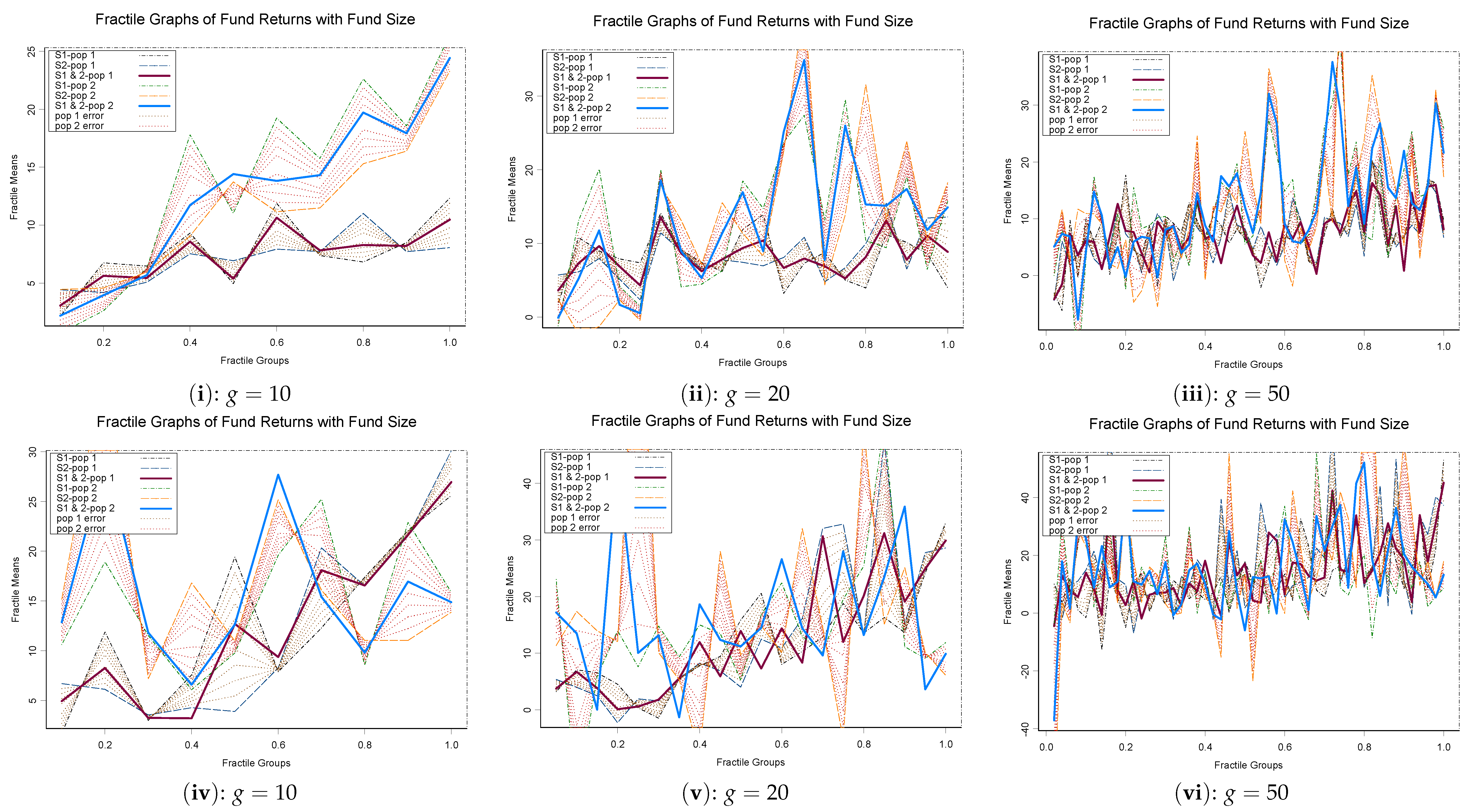
Although we do reject $H_0:F=G$ that the return distributions for private and public equity are the same with the BGX smooth test (Bera et al. 2013), there is no indication of the nature of departure from $H_0$ using the traditional tests such as Kolmogorov–Smirnov or Cramér–von Mises type tests (see

Table 1. This table shows the omnibus test statistic for distribution comparison (modified Kolmogorov–Smirnov and Cramér–von Mises statistics) and corresponding 0.1% critical value reported in R.B.D${}^{\prime }$ Agostino and M.A.Stephens. Goodness-of-Fit Techniques. NewYork: Marcel Dekker, 1986.

Test	Modified KS	Modified CvM
T* Statistic (All–all)	6.96	16.47
T* Statistic (NoYield–All)	9.12	21.85
T* Statistic (NoYield–liq.)	6.31	9.67
T* Statistic (NoYield–pre96.)	8.7	16.62
T* Statistic(VC-LBO)	2.04	2.38
Critical Upper 0.1%	1.95	1.167

). We use a modified version of Fractile Graphical Analysis method (Mahalanobis 1961) to test the overall distribution of returns conditional on the size of the fund for private and public equity. We include size of assets under management (AUM) as a possible covariate, as several studies found an impact of fund size on return distribution but not the sequence number (Gompers and Lerner 2000; Kaplan and Schoar 2005; Phalippou and Zollo 2005). Figure 2i–vi depict the kernel density functions and the empirical distribution functions of public and private equity returns under different restrictions. More precisely, Figure 2i,iv represent unconditional distributions of public and private equity returns, Figure 2ii,v show the returns for those public equity with no yield or dividend distribution and private equity, and Figure 2iii,vi represent distributions for venture capital (VC) and leveraged buyout (LBO), respectively. Figure 3i–iii represent the fractile graphs with number of fractile groups $g=10,20$, and 50 and depicts the difference between private and public equity mutual funds. In Figure 3i–iii, the blue (top) solid line represents the private equity funds returns for each size fractile group, whereas the red (bottom) line represents the public equity returns conditioned on fractile groups of fund size. The shaded area around the line represents the estimation uncertainty or dispersion, i.e., the bootstrapped standard error at each fractile group mean.

As we observe with higher number of fractile (or rank) groups of sizes, the separation area between the two graphs, represented by the blue (top) and the red (bottom) lines, is more fragmented. This also make it increasingly difficult to conclude whether the distributions are different overall. Hence, we would need some more tangible analytical or simulation based hypothesis testing methodology to test for separation of the two fractile graphs. Similar analysis is also done between return distributions of VC and LBO returns in Figure 3iv–vi. After conditioning for size, the return distributions look increasingly similar, with neither VC nor LBO seeming to dominate across the fractile groups based on fund size.

Unfortunately, standard tests of goodness-of-fit like Kolmogorov–Smirnov (K-S) and Cramér–von Mises (C-vM) (reported in Table 1) do not provide us with the exact nature of such departures from the null hypothesis of equality of two distributions. The data show that, not only is there a difference in both the location and scale of the distribution, but also that the shape parameters of the distribution might be different. In order for us to numerically compare the returns distribution of private equity funds with public equity funds, we investigate the summary statistics of each of the groups.

Table 2. Summary statistics of returns of public and private equity funds with different restrictions.

Variable	Obs.	Mean	Median	Std. Dev.	1st Q.	3rd Q.	Coef. Skew	Excs. Kurt	Sharpe Ratio
Public (full)	10,103	10.19	11.51	22.69	−6.63	24.4	0.813	3.93	0.45
Public (No yield)	5635	7.59	6.65	26.58	−12.31	23.19	1.079	3.54	0.29
Private (full)	1714	13.36	6.28	42.25	−1.14	16.28	9.44	137.61	0.32
Private (liq.)	491	11.15	8.79	20.05	1.39	16.13	2.49	13.01	0.56
Private (pre96)	840	15.11	9.85	37.13	2.04	18.4	12.31	238.93	0.41
VC(pre96)	610	15.27	18.7	41.59	1.43	17.07	11.97	208.29	0.38
LBO (pre96)	206	15.27	12.17	22.32	4.225	22.43	1.65	9.13	0.68

provides a sample size of public equity fund to n = 10,103 (full sample after 1996 until 2002) and $n=5635$ for mutual funds with no yields. The size of the sample of private equity funds are $m=1714$ (full sample) and $m=491$ (for liquidated funds), respectively. As we apply the sample size selection methods for comparing distributions, we have restricted our sample for private equity to only the ones that are more mature or spent some time after inception. We restrict our attention to only those private equity funds with fund inception year before 1996 $\left(m=840\right)$. Our working assumption is that private funds that are mature will start to show some cash flow from 6 years after inception (Kaplan and Schoar 2005).

We report the results of the individual and group F-tests in

Table 3. Hypothesis tests based the FGA using bootstrapped standard errors for private and public equity and between venture capital and buyout funds with p-values in parentheses for the asymptotic tests (A). We also look at the actual size of nominal 5% level test to see possible size distortion with the distribution under $H_0$ on the column header. (A) Asymptotic tests of normalized error area and the area of separation (p-values in parentheses); (B) actual size of the 5% FGA tests using bootstrap covariance matrix $(repl.=500, Boots.=5000)$.

(A)
#Fractile Groups	Private Equity	Public Equity	Area of Separation	Overall F-Test	VC-Buyout F-Test
Under $H_0:m_1\left(x\right)=m_2\left(x\right)$	$m{\Gamma }_{12}^2\sim {\chi }_g^2$	$m{\Gamma }_{34}^2\sim {\chi }_g^2$	$2m{\Gamma }_{*}^2\sim {\chi }_{2g}^2$	$\frac{2{\Gamma }_{*}^2}{\left({\Gamma }_{12}^2+{\Gamma }_{34}^2\right)}\sim F_{2g,g}$
$g=10$	8.11	10.11	95.72 ***	10.51 ***	0.774
	$\left(0.62\right)$	$\left(0.43\right)$	$\left(0.0\right)$	$\left(0.0\right)$	$\left(0.65\right)$
$g=20$	19.51	23.97	104.35 ***	4.8 ***	1.53
	$\left(0.49\right)$	$\left(0.24\right)$	$\left(0.0\right)$	$\left(0.0\right)$	$\left(0.13\right)$
$g=50$	56.81	49.4	146.24 ***	2.75 ***	1.84 ***
	$\left(0.24\right)$	$\left(0.5\right)$	$\left(0.0\right)$	$\left(0.0\right)$	$\left(0.00\right)$
(B)
Size of the Tests	Private Equity	Public Equity	Area of Separation	Overall F-Test
Under $H_0:m_1\left(x\right)=m_2\left(x\right)$	$m{\Gamma }_{12}^2\sim {\chi }_g^2$	$m{\Gamma }_{34}^2\sim {\chi }_g^2$	$2m{\Gamma }_{*}^2\sim {\chi }_{2g}^2$	$\frac{2{\Gamma }_{*}^2}{\left({\Gamma }_{12}^2+{\Gamma }_{34}^2\right)}\sim F_{2g,g}$
$g=10$	$0.05$	$0.04$	$0.05$	$0.06$
$g=20$	$0.05$	$0.05$	$0.06$	$0.04$
$g=50$	$0.05$	$0.05$	$0.05$	$0.05$

*** significant at 1%, ** significant at 5%, * significant at 10%.

A, if we want to test all the conditional fractile means jointly. We observe that the results of the overall F-tests and tests for error areas of the two fractile graphs give similar results for different values of $g.$ Individually, after adjusting for the ranks of the fund size, the adjusted error areas of the fractile graphs of both private and public returns are distributed as ${\chi }^2$ with $g$ degrees of freedom. This signifies that that the FGA model is indeed a good fit for both public and private equity returns. The test for the area of separation, however, indicates that at a $5\%$ level of significance, there is a difference between the two fractile graphs. The overall F-test for fractile graphs helps us to compare the conditional fractile means jointly, and we infer that at the $5\%$ level, at least one of the size fractile means of returns is different between the groups. We can conclude that the public and private equity fund distributions are different using the F-test, or, adjusting for the fractile groups of rank, private and public equity fund returns are different using a $5\%$ level of significance. This implies that there might be some abnormal returns at each size fractile, hence, size alone or “money chasing deals” cannot explain the difference of returns (Gompers and Lerner 2000; Phalippou and Zollo 2005).

However, although it adjusts for the fractiles of the covariate size, the overall F-test do not give us any indication of the directions of departures from the null hypothesis, very much like the $omnibus$ test (Kolmogorov–Smirnov and Cramér–von Mises tests). We further note that tests based on fractile graphs provide a non-parametric alternative to tests based on functions of the first two moments (or Sharpe ratio). Unlike the tests based on moments, we also adjust for the conditional fractile groups of the fund size (Ledoit and Wolf 2008).

We also compare the actual size of the tests of hypothesis using bootstrap covariance matrices to normalize the test statistic. We have simulated the test statistic by drawing the same first and second samples of the X and Y variables and repeated it $r=500$ times; the bootstrap replication was $B=5000$ to estimate the covariance matrix. In Table 3B, we observe that the test sizes of all the tests were pretty close to the $5\%$ nominal level test (minimum being $0.04$ to maximum of $0.06$), although there are some finite sample size distortions.

The results are robust to fatter tailed and potentially skewed distributions (such as private equity returns, as is shown in Figure 2). This is mainly because we transform the original data to their probability integral transform, which has a range (0,1). Under the null hypothesis of equality of distributions, the test statistic would be distributed as U(0,1) (Bera et al. 2013). One reason for using 1999 data was for comparison purpose with public and private equity data cited in past research.

A problem with omnibus test methods, such as Kolmogorov–Smirnov and Cramér–von Mises type tests that have power in all directions, is that they have weak power against more directional alternatives. Hence, we might fail to reject a hypothesis that is indeed false. In our case here, we do reject the null hypothesis of equality of the distributions of private and public equity returns. Therefore, we can believe beyond reasonable doubt the two distributions are indeed different overall. However, the same thing cannot be said about all parts of the distributions measured by subsets of fractile means or graphs (see Figure 3i–iii). It appears that for $g=10$ and $g=20$ fractile groups, there is a difference between private and public equity returns after the 40th percentile of net asset for public equity funds or total commitment size of private equity funds (or top $60\%$ of fund sizes). It is, however, more difficult to separate out for the bottom 40% of the funds, or when $g=50$, due to the wide variation of the fractile means.

As discussed before, the choice of number of groups g and group size m are similar to a bandwidth selection problem. This can also be construed as a bias variance trade-off or the high or low frequency trade-off. For higher numbers of groups g (as we see in Table 3A,B, Figure 3), we pick up more local variation and noise. The bigger the sample size is, the more the number of groups g can be selected.

6. Introducing Fractile Regression

Although we can compare overall unconditional distributions or conditional distributions on certain covariates using fractile based methods, one of the objectives in this paper is to look at the age-old problem of the effect of the covariates on distributions. Linear regression has always been the cornerstone of such an analysis where we investigate the effects of the x-variables or covariates on the response variable y. A very simple example of that could be the effect of educational qualification measured in years of education on income or future income. It could be argued that educational qualification is a proxy for ability, hence higher educational qualification would lead to higher earnings. However, performing simple linear regression on this somewhat naive model of “Returns to Education” misses some major parts of the story. First, the story of endogeneity, that is to say, it is very rare that education is randomly assigned, so individuals choose education based on their ability and opportunity cost. Hence, it would be wrong to assign the credit of higher income solely to education; there could quite a few omitted variables. In fact, the error term $\epsilon$ in the population linear regression model, i.e.,

$$y={\beta }_0+{\beta }_{1}x+\epsilon$$

where y is, say, log of income and x is the number of years of education, ${\beta }_0$ and ${\beta }_1$ are the partial regression coefficients. Here, the disturbance term $\epsilon$ might be correlated with the independent variable x—a problem often times referred to as “endogeneity” in Econometrics. However, the problem we are trying to address is not directly related to endogeneity, but the other aspect of the story missed by simple linear regression. It is very likely that people with high ability or high educational qualification might command a much higher salary for one extra year of education compared with someone with low ability or education. Linear regression fails to capture this “differential” treatment of the covariates or, in particular, “fractiles of the covariates”. Therefore, instead of looking at regression of y on x, we should be looking at the regression of Y grouped according to fractiles of X, i.e., we can answer the question for the bottom 10% of educational qualification in the society—what is the effect of one more year of education, all else remaining the same.

To motivate for fractile regression, let us think of a regression function of Y on $X=x$ as

$$m\left(x\right)=E\left[Y|X=x\right]$$

(12)

Let $F\left(x\right)$ be the marginal cumulative distribution function (CDF) of X with a density function (PDF) $f\left(x\right).$ We can show that the regression function is invariant under a strictly monotonic transformation of the covariate X to its probability integral transform (PIT), $F\left(x\right).$ Following Rao and Zhao (1996), let us define the following regression function of Y on X as

$$\begin{array}{cc}\hfill r\left(u\right)& =E\left[Y|F\left(X\right)=u\right]\hfill \\ \hfill & \Rightarrow r\left(u\right)=E\left[Y|X=F^{-1}\left(u\right)\right]=m\left(F^{-1}\left(u\right)\right),0\le u\le 1.\hfill \end{array}$$

(13)

The partial regression coefficients of $r\left(u\right)$ are given by

$$\frac{\partial r\left(u\right)}{\partial u}=\frac{\partial m\left(x\right)}{\partial x}.\frac{\partial F^{-1}\left(u\right)}{\partial u}=m^{\prime }\left(x\right)\frac{1}{f\left(x\right)}\frac{dx}{du},$$

(14)

where we divide the non-parametric regression coefficients by the density function evaluated at $x.$ One interpretation of that could be the regression coefficients are weighted less where the density of the covariate is low. As we can imagine now, that FGA is not just the “Prehistory of Bootstrap” (Hall 2003) but the “Prehistory of Inference on Non-parametric Regression” as well. Several asymptotic properties of fractile regression functions are proved in Bera et al. (2021). In particular, results in Bera et al. (2021) imply that it is sufficient to work with the probability integral transforms of the Y variable after conditioning for the rank of the X variable, where scaled rank (probability intergral transform) of Y conditioned on the rank of X has been referred to as the induced order statistics (Bhattacharya 1974) or concomitant of order statistics (David 1973).

7. Fractile Regression: Application on Pre- and Post-Tax Mutual Fund Inflow Distributions

There are several examples where we can use FGA based techniques. As discussed previously, examples include male–female or younger–older workers wage gap with respect to returns to education; productivity gap between large and small firms or productivity with respect to firm size; difference on returns to equity with firm size; income distribution of different ethnic groups or countries with respect to age, etc. Our nomenclature, however, is distinct from the Cumulative Fractile Regression Function proposed by Rao and Zhao (1995), which deals with empirical cumulative quantile regression functions, although we also provide area under fractile groups of covariates.

For performing this test of comparison of distributions, we use the two sample version of the Neyman (1937) smooth test procedure as proposed in Bera et al. (2013) based on Rao score (RS) principles. If we go to the problem of testing $H_0:F=G$, we need to modify the original smooth test, as both F and G are unknown. If $F\left(.\right)$ were known, we can construct a new random variable $Z_j=F\left(Y_j\right),$ $j=1,2,\dots ,m.$

For the two sample case with unknown F and G, the smooth test statistic is

$$\begin{array}{cc}\hfill {\Psi }_k^2& =\sum _{l=1}^k{u}_l^2,u_l=\frac{1}{\sqrt{m}}\sum _{j=1}^m{\pi }_l\left(z_j\right),l=1,2,\dots ,k\hfill \\ \hfill z_j& =F\left(y_j\right)={\int }_{-\infty }^{y_j}f\left(\omega \right)d\omega ,j=1,2,\dots ,m.\hfill \end{array}$$

Under $H_0:F=G,{\Psi }_k^2\stackrel{D}{\to }{\chi }_k^2,$ where ${\pi }_l$ are normalized Legendre polynomials.

The test has k components. Each component provides information regarding specific departures from $H_0:F=G.$ However, in practice $F\left(.\right)$ is unknown. We use the empirical distribution function,

$$\begin{array}{cc}\hfill F_n\left(x\right)& =\frac{1}{n}\sum _{i=1}^{n}I\left(X_i\le x\right),{\widehat{z}}_j=F_n\left(y_j\right)\hfill \\ \hfill {\widehat{\Psi }}_k^2& =\sum _{l=1}^k\frac{1}{m}{\left[\sum _{j=1}^m{\pi }_l\left({\widehat{z}}_j\right)\right]}^2.\hfill \end{array}$$

We used a cross-validation type procedure to select sample sizes for the two samples (Bera et al. 2013; Cao et al. 2017).

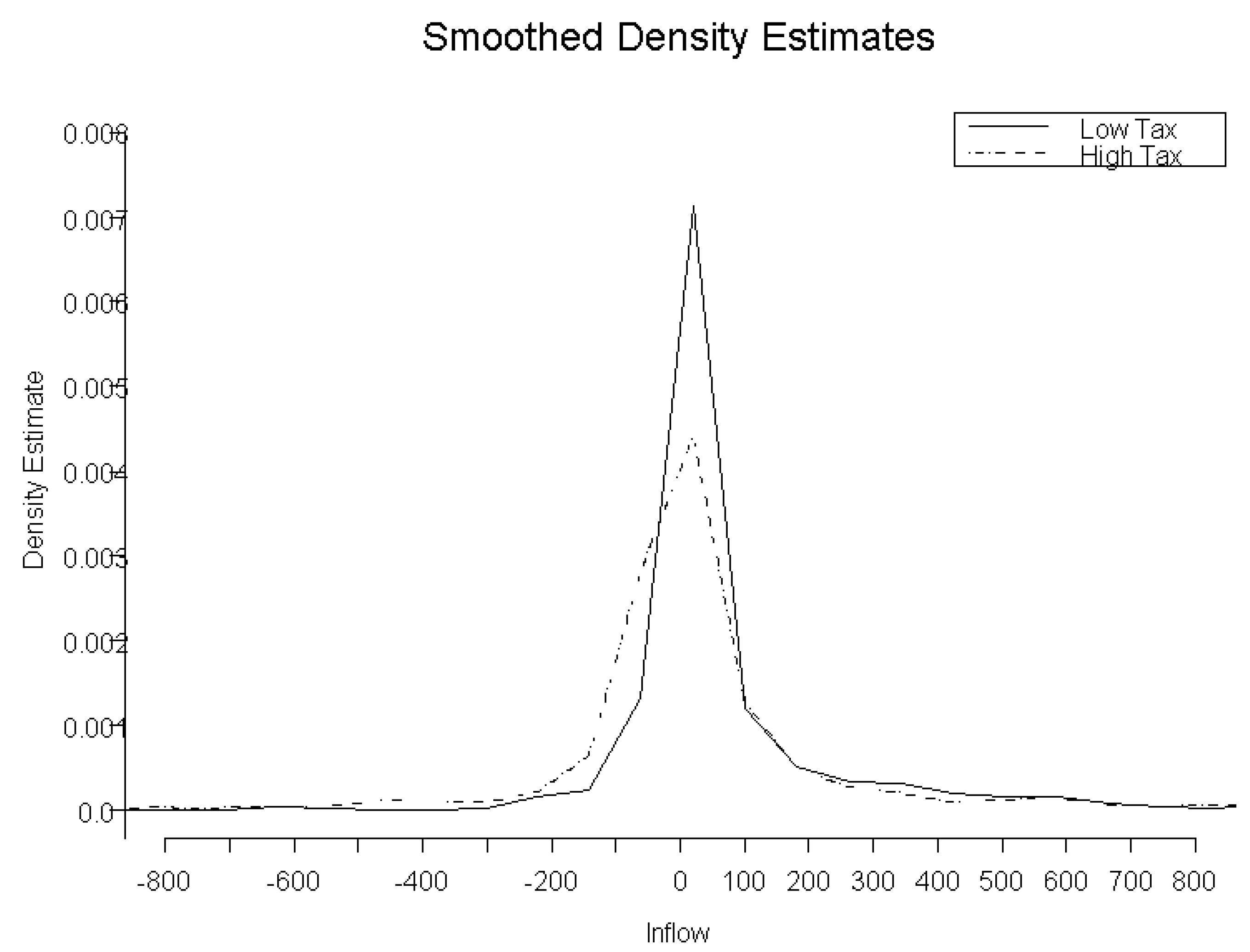
One of the main problems we would investigate is the distributions of mutual fund inflows with before and after taxes with returns as covariate (Bergstresser and Poterba 2002).

Table 4. Summary statistics for fund inflows.

Variable	Obs.	Mean	Median	Std. Dev.
Low Tax	864	187.43	12.15	782.77
High Tax	812	211.83	0.45	1427.04
Min.	1st Q.	3rd Q.	Max.	Coef. Skew	Excs. Kurt
−3686	−2.325	93.625	10,454.5	7.019	69.15
−3961	−25.6	66.025	28,651.3	11.888	204.738

and

Table 5. Goodness-of-fit statistics based on the EDF.

Test	KS	CvM
Statistic (T*)	5.3560346	9.371912
Critical Upper 0.1%	1.95	1.167

show that the mutual fund inflow distributions are different before and after taxes with past year returns as covariate using Kolmogorov–Smirnov and Cramér–von Mises tests (Bergstresser and Poterba 2002). This might be because of the well-known “return chasing” behavior among investors and excessive risk taking among fund managers (Chevalier and Ellison 1997). We want to investigate how these distributions are different when we control for the fractiles of returns, hence we can predict the mutual fund inflow based on pre-tax or post-tax return information. This paper documents that mutual funds with heavily taxed returns have lower subsequent inflows compared to ones with lower tax burdens. Our objective is to see if there is evidence in the inflow distributions to show whether higher moments including volatility or skewness and kurtosis terms of inflow distributions are affected by tax exposure. Bergstresser and Poterba (2002) considered US domestic equity mutual funds data on January Releases from Morningstar Principia database with some conditions from 1993–1999.

For our current illustrative exposition, we will only focus on the 1999 equity mutual fund returns and inflow data with similar characteristics (Figure 4). The summary statistics in Table 4 show that there seems to be a difference between the means of the inflow distributions of mutual funds with high and low tax exposures. Bergstresser and Poterba (2002) found that after-tax returns do indeed have more influence on cash inflows on mutual funds; however, they did not test whether higher order moments of the inflow distribution are affected by after tax returns.

We tend to reject $H_0:F=G$ with the K-S and C-vM tests in Table 5, but there is no indication of the nature of departure from $H_0.$ Using the BGX smooth test for the full sample, we observe that pre-tax and post-tax mutual fund inflow distributions are indeed significantly different for higher order moments (

Table 6. Smooth statistics and p-values (whole sample).

${\mathit{\Psi }}_4^2$	${\mathit{u}}_1^2$	${\mathit{u}}_2^2$	${\mathit{u}}_3^2$	${\mathit{u}}_4^2$
192.33 ***	39.16 ***	111.19 ***	6.74 **	2.01
(0.0)	(0.0)	(0.0)	(0.0094)	(0.1559)

*** significant at 1%, ** significant at 5%, * significant at 10%.

).

To reduce the effect of the relative sample sizes, we took a random sample of the inflow distribution from higher tax returns and recomputed the smooth test statistics in

Table 7. Smooth statistics and p-values (sample $m=324$).

Residuals with Returns	${\mathit{\Psi }}^2$	${\mathit{u}}_1^2$	${\mathit{u}}_2^2$	${\mathit{u}}_3^2$	${\mathit{u}}_4^2$
Unadjusted	72.37 ***	35.81 ***	34.77 ***	0.76	1.04
	$\left(0.00\right)$	$\left(0.00\right)$	$\left(0.00\right)$	$\left(0.38\right)$	$\left(0.31\right)$
OLS	218.45 ***	5.25 **	117.84 ***	13.18 ***	82.18 ***
	$\left(0.00\right)$	$\left(0.02\right)$	$\left(0.00\right)$	$\left(0.00\right)$	$\left(0.00\right)$
Median Regression	21.93 ***	0.00	6.76 ***	12.56 ***	2.62
	$\left(0.00\right)$	$\left(0.96\right)$	$\left(0.01\right)$	$\left(0.00\right)$	$\left(0.11\right)$
Fractile Regression	170.76 ***	1.46	115.00 ***	8.09 ***	46.22 ***
	$\left(0.00\right)$	$\left(0.23\right)$	$\left(0.00\right)$	$\left(0.00\right)$	$\left(0.00\right)$
Median-Fractile	45.94 ***	0.01	27.20 ***	13.05 ***	5.68 **
	$\left(0.00\right)$	$\left(0.93\right)$	$\left(0.00\right)$	$\left(0.00\right)$	$\left(0.02\right)$

*** significant at 1%, ** significant at 5%, * significant at 10%.

, with the mutual inflows unadjusted for returns, then residuals from OLS, median regression, fractile regression and, finally, a median regression on the fractiles of x.

One obvious argument in this case is how to choose the mutual funds that have a comparatively high tax exposure; the only way to address this problem is to make fractile or rank groups of the returns. A detailed inspection of Table 7 reveals quite a few facets of the distribution of mutual fund inflows once adjusted for the covariate, in this case, past years returns. We also see that the type of regression we use to adjust for the effect of mutual fund returns does indeed make a difference in the distribution of inflows with high and low tax exposure. From Table 7, we observe that the unadjusted inflow distribution for mutual funds with high and low tax exposure differs significantly in the first ($u_1^2=35.81)$ and second $\left(u_2^2=34.77\right)$ moment components. However, past years’ mutual fund returns is the most important factor in determining mutual fund inflows (regression results not shown here, refer to Bergstresser and Poterba 2002). Hence, to compare the explanatory power of high and low tax exposure of the returns in explaining mutual fund inflows, we need to adjust for the variation in returns.

If we take ordinary least squares residuals (Bergstresser and Poterba 2002), the distribution of inflows adjusted for returns in the high and low tax exposure groups are distinctly different from each other in the direction of each of the first four moments (Table 7). This result could be due to the existence of extreme observations in the data. In order to reduce the effect of outliers, we can use median regression (quantile regression for the 50th percentile). We observe that the two adjusted distributions now only differ in the direction of the second and third moments ( $u_2^2=6.76$ and $u_3^2=12.56$). This could be due to the difference in the risk preference and asymmetric loss function of the investors in those mutual funds. However, this result could also be an artifact of the possibility that the distributions of returns are distinctly different between the mutual funds with low tax exposure and those with high tax exposure.

Therefore, in order to make the two groups comparable, we have to standardize the covariates. Hence, we look at the residuals using the proposed fractile regression method without using any smoothing techniques. The returns adjusted inflow distribution differs in the directions of the second, third, and fourth moments ($u_2^2=115.00$, $u_3^2=8.10$, and $u_4^2=46.22$), although the departure in the direction of the fourth moment is much reduced ($u_4^2=5.68$) and is only slightly significant if we combine quantile and fractile regressions.

We can apply FGA based methods for determining the nature of departure of wages across genders or ethnic groups after adjusting for educational qualifications and training. To account for the endogeneity in schooling, GMM technique has been used in panel data to investigate how OLS regression might overestimate the gender gap (Hansen and Wahlberg 2005). This, however, does not address the fact that the gap might be different controlling for percentiles of schooling.

8. Epilogue: Conclusions and Future Research

We re-evaluate Mahalanobis’ FGA and his contribution to the statistics and econometrics literature, as a precursor to k-nearest neighbor regression techniques. One of our main objectives in this paper is to introduce a new form of non-parametric regression, namely, fractile regression, aimed towards comparing distributions of induced order statistics or fractiles of concomitant variables. We highlighted how FGA techniques can be used to compare distribution functions after conditioning for ranks of a covariate to compare across different regimes, be it in time or space, by standardizing the reference points to the unit interval, through examples in Empirical Finance, including introducing a new F-test of goodness-of-fit as an application of FGA for comparing the distributions of private and public equity returns (Kaplan and Schoar 2005; Moskowitz and Vissing-Jorgensen 2002) and distribution of mutual fund inflows with pre-tax and after tax returns (Bergstresser and Poterba 2002). These illustrative examples demonstrate that we can expand the BGX smooth test techniques based on the Rao score principle of testing to compare distributions of returns or inflows by conditioning on concomitant variables without imposing distribution restrictions or linearity. In ongoing and future research, we want to establish asymptotic properties of fractile regression estimates and applications in asset pricing and credit risk modeling with “scores” to accommodate for multiple covariates (Bera et al. 2021).

References

- Altman, Naomi S. 1992. An Introduction to Kernel and Nearest-Neighbor Nonparametric Regression. The American Statistician 46: 175–85. [Google Scholar]
- Bera, Anil K., Aurobindo Ghosh, and Zhijie Xiao. 2013. A Smooth Test for the Equality of Distributions. Econometric Theory 29: 419–46. [Google Scholar] [CrossRef]
- Bera, Anil K., Aurobindo Ghosh, and Zhijie Xiao. 2021. Fractile Regression: Theory and Applications. Working Paper. Singapore: Singapore Management University. [Google Scholar]
- Bera, Anil Kumar, and Aurobindo Ghosh. 2001. Neyman’s Smooth Test and Its Applications in Econometrics. In Handbook of Applied Econometrics and Statistical Inference. Edited by Aman Ullah, Alan Wan and Anoop Chaturvedi. New York: Marcel Dekker, pp. 177–249. [Google Scholar]
- Bergstresser, Daniel, and James Poterba. 2002. Do after-tax returns affect mutual fund inflows? Journal of Financial Economics 63: 381–414. [Google Scholar] [CrossRef]
- Bhattacharya, Prodyot K. 1974. Convergence of sample paths of normalized sums of induced order statistics. Annals of Statistics 2: 1034–39. [Google Scholar] [CrossRef]
- Cao, Jerry, Aurobindo Ghosh, and Jeremy Goh. 2017. Risking Returns: Moving from Public to Private Equity. Working Paper. Singapore: Singapore Management University. [Google Scholar]
- Chevalier, Judith, and Glenn Ellison. 1997. Risk Taking by Mutual Funds as a Response to Incentives. Journal of Political Economy 105: 1167–200. [Google Scholar] [CrossRef]
- David, Herbert A. 1973. Concomitants of order statistics. Bulletin of the International Statistical Institute 45: 295–300. [Google Scholar]
- Efron, Bradley. 1982. The Jackknife, the Boostrap and Other Resampling Plans. Philadelphia: SIAM. [Google Scholar]
- Ghosh, Jayanta K., Pulakesh Maiti, T. Jagannadha Rao, and Bikash K. Sinha. 1999. Evolution of Statistics in India. International Statistical Review/Revue Internationale de Statistique 67: 13–34. [Google Scholar]
- Ghosh, Jayanta K. 2001. Prasanta Chandra Mahalanobis. In Statisticians of the Century. Edited by Chris Heyde and Eugene Seneta. New York: Springer. [Google Scholar]
- Ghosh, Jayanta Kumar. 1994. Mahalanobis and the art and science of statistics: The Early Days. Indian Journal of History of Science 29: 89–98. [Google Scholar]
- Gompers, Paul, and Josh Lerner. 2000. Money chasing deals? The impact of fund inflows on private equity valuations. Journal of Financial Economics 55: 281–325. [Google Scholar] [CrossRef]
- Gottschalg, Oliver, Ludovic Phalippou, and Maurizio G. Zollo. 2003. Performance of Private Equity Funds: Another Puzzle? Working Paper 2003/93/SM/ACGRD 3. Fontainebleau: INSEAD. [Google Scholar]
- Hall, Peter. 2003. A Short Prehistory of the Bootstrap. Statistical Science 18: 158–67. [Google Scholar] [CrossRef]
- Hansen, Jorgen, and Roger Wahlberg. 2005. Endogenous schooling and the distribution of the gender wage gap. Empirical Economics 30: 1–22. [Google Scholar] [CrossRef]
- ISI. 1997. Lekhon: The Mouthpiece of Indian Statistical Institute Club. Edited by Prasanta Chandra Mahalanobis. Calcutta: Indian Statistical Institute. [Google Scholar]
- Iyengar, N. S., and Nikhilesh Bhattacharya. 1965. Some Observations on Fractile Graphical Analysis. Econometrica 33: 644–45. [Google Scholar] [CrossRef]
- Kaplan, Steven N., and Antoninette Schoar. 2005. Private Equity Performance: Returns, Persistence and Capital Flows. The Journal of Finance 60: 1791–823. [Google Scholar] [CrossRef]
- Koenker, Roger, and Gilbert Bassett Jr. 1978. Regression Quantiles. Econometrica 46: 33–50. [Google Scholar] [CrossRef]
- Ledoit, Olivier, and Michael Wolf. 2008. Robust Performance Hypothesis Testing with the Sharpe Ratio. Journal of Empirical Finance 15: 850–59. [Google Scholar] [CrossRef]
- Mahalanobis, P. C. 1958. A Method of Fractile Graphical Analysis with Some Surmises of Results. Calcutta: Transactions of the Bose Research Institute. [Google Scholar]
- Mahalanobis, Prasanta C. 1953. Some Observations on the Process of Growth of National Income. Sankhya 12: 307–12. [Google Scholar]
- Mahalanobis, Prasanta C. 1961. A Method of Fractile Graphical Analysis. Econometrica 28: 325–51. [Google Scholar] [CrossRef]
- Mahalanobis, Prasanta C. 1969. Extensions of Fractile Graphical Analysis. In Proceedings of the International Conference on Quality Control. Tokyo: Japan. [Google Scholar]
- Mahalanobis, Prasanta C. 1970. Extensions of Fractile Graphical Analysis to Higher Dimensional Data. In Essays in Probability and Statistics. Edited by Raj Chandra Bose. Chapel Hill: University of North Carolina Press. [Google Scholar]
- Moskowitz, Tobias J., and Annette Vissing-Jorgensen. 2002. The Return to Entrepreneurial Investment: A Private Equity Premium Puzzle? American Economic Review 92: 745–78. [Google Scholar] [CrossRef]
- Neyman, Jerzy. 1937. “Smooth test” for goodness of fit. Skandinaviske Aktuarietidskrift 20: 150–99. [Google Scholar]
- Phalippou, Ludovic, and Maurizio Zollo. 2005. What Drives Private Equity Fund Performance? Working Paper, R&D Group. Fontainebleau: INSEAD. [Google Scholar]
- Rao, Calyumpudi Radhakrishna. 1974. Mahalanobis Era in Statistics. Sankhya 35: 4. [Google Scholar]
- Rao, Calyumpudi Radhakrishna. 1993a. Prashanta Chandra Mahalanobis: June 29,1893–June 28, 1972. The IMS Bulletin 22: 593–97. [Google Scholar]
- Rao, Calyumpudi Radhakrishna. 1993b. Statistics must have a purpose: The Mahalanobis Dictum. Sankhyā 55: 331–49. [Google Scholar]
- Rao, Calyumpudi Radhakrishna, and Lincheng Zhao. 1995. Convergence Theorems for Empirical Cumulative Quantile Regression Functions. Mathematical Methods of Statistics 4: 81–91. [Google Scholar]
- Rao, Calyumpudi Radhakrishna, and Lincheng Zhao. 1996. Law of Iterated Logarithm for Empirical Cumulative Quantile Regression Functions. Statistica Sinica 6: 693–702. [Google Scholar]
- Schuster, Eugene F. 1972. Joint asymptotic distribution of the estimated regression function at a finite number of distinct points. Annals of Mathematical Statistics 43: 84–88. [Google Scholar] [CrossRef]
- Sen, Bodhisattva. 2005. Estimation and Comparison of Fractile Graphs Using Kernel Smoothing Techniques. Sankhyā 67: 305–34. [Google Scholar]
- Sen, Bodhisattva, and Prabal Chaudhuri. 2011. On Fractile Transformation of Covariates in Regression. Journal of the American Statistical Association 107: 349–61. [Google Scholar] [CrossRef]
- Srinivasan, T. Nilakanta. 1996. Professor Mahalanobis and Economics. In Prashanta Chandra Mahalanobis: A Biography. Edited by Ashok Rudra. New Delhi: Oxford University Press, Chp. 11. pp. 224–52. [Google Scholar]
- Stute, Winfried. 1984. Asymptotic Normality of Nearest Neighbor Regression Function Estimates. The Annals of Statistics 12: 917–26. [Google Scholar] [CrossRef]
- Yang, Shie-Shien. 1981. Linear functions of concomitants of order statistics with applications to nonparametric estimation of a regression function. Journal of the American Statistical Association 76: 658–62. [Google Scholar] [CrossRef]
Figure 1.
(A) Fractile graphs give the individual and combined fractile group means from samples drawn from the same population. The error area between the graphs gives an indication of the variation, whereas the solid line G12 gives the average estimate with 20 fractile groups. (B) Interprenetrating subsamples G1 and G2 are drawn from population 1, and G3 and G4 are drawn from population 2. Combined fractile graph G12 represents the fractile means of population 1, whereas G34 is for population 2. In addition, the error area between G1 and G2, and that between G3 and G4, gives indication of the variation of the combined graph from each population. The area of separation is the space between the two combined graphs, which indicates how different the two populations are after controlling for the rank of some coviarate.
Figure 2.
Kernel density functions (i,ii) and empirical distribution functions (iv,v) of unadjusted annual public equity funds returns (1996–2002) and private equity internal rates of returns (inception before 1996); (iii,vi) are the kernel density estimates of venture capital (VC) and buyout funds (LBO).
Figure 3.
Fractile graphs (Mahalanobis 1961) for different number fractile groups for public and private equity (–) and between venture capital (VC) and buyout fund (LBO) returns (–).
Figure 4.
Inflow of mutual funds.