Saddlepoint Method for Pricing European Options under Markov-Switching Heston’s Stochastic Volatility Model

Abstract

This paper evaluates the prices of European-style options when dynamics of the underlying asset is assumed to follow a Markov-switching Heston’s stochastic volatility model. Under this framework, the expected return and the long-term mean of the variance of the underlying asset rely on states of the economy modeled by a continuous-time Markov chain. There is evidence that the Markov-switching Heston’s stochastic volatility model performs well in capturing major events affecting price dynamics. However, due to the nature of the model, analytic solutions for the prices of options or other financial derivatives do not exist. By means of the saddlepoint method, an analytic approximation for European-style option price is presented. The saddlepoint method gives an effective approximation to option prices under the Markov-switching Heston’s stochastic volatility model.

1. Introduction

It is well documented that the stochastic volatility (SV) models take the volatility smile effect into account in the real markets. Needless to say, the SV models are more realistic than the standard Black–Scholes model. Nevertheless, Vo (2009) conducted an empirical study on a Markov-switching stochastic volatility model and showed that the behaviour of crude oil price is well explained under the Markov-switching SV model. A significant regime-switching effect on the oil markets is well documented and their numerical results reveal that the forecasting power of the SV model with Markov switching outperforms its non-switching counterpart. The empirical study also finds that the SV model with Markov switching is able to capture large shocks of the oil markets well. These advantages of empirical findings give us a motivation to pricing options under SV models with Markov switching.

This paper shows how to price a European-style option in Markov-switching Heston’s stochastic volatility model. Under the Markov-switching Heston’s stochastic volatility model, the key parameters of the model follow Markov chains which switch from a state to another state as time evolves. The Markov-switching (regime-switching) behaviour could reflect the dynamic preferences and time-varying beliefs of traders or the changing levels of economy activities. In general, the Markov chain is unobservable and the chain is modeled by a stochastic differential equation (SDE). Zhu et al. (2012) derive an explicit European option pricing formulas in a two-state regime by solving a couple of partial differential equations (PDEs) using the Fourier transform method. Chan and Zhu (2021b) obtain a closed-form formulas of Lookback options under a Markov-switching Wiener process. Chan and Zhu (2015) derive a closed-form formula of American convertible bonds in a Black–Scholes–Merton’s model with regime switching. Chan and Zhu (2021a) obtain an analytic approach for pricing American options with Markov switching. Elliott et al. (2013) price options under the CEV model with Markov switching. Chan and Zhu (2015) consider a homotopy analysis method to price barrier options under the Markov-switching Wiener process. Elliott et al. (2014) use a quadratic approximation approach to price barrier options under the Markov switching model. Bollen (1998) calculates a European option price under the Markov switching model via a binomial tree. Hardy (2001) proposes a recursive algorithm to price European options under the Markov switching model. Duan et al. (2002) use a lattice-approximation method to price European-style and American-style options under the Markov switching model. Boyle and Draviam (2007) use a finite difference scheme to price exotic options under the Markov switching model. Li et al. (2012) derive the bounds of exotic option price using semidefinite programming (SDP) under the Markov switching model. Lu and Putri (2020) evaluate Markov-switching American option via Laplace transform. Egami and Kevkhishvili (2020) simplify an optimal stopping problem for a two-state Markov-switching model to a pair of no-switching optimal stopping problems. Elliott and Lian (2013) investigate the pricing of variance swaps under a Markov-switching stochastic volatility model.

The saddlepoint method has been widely used in approximating the probability distribution of the partial sum of independent random variables since it was proposed by Daniels in 1954. In this paper, instead of approximating distributions, we use the Lugannani and Rice (LR) formula (Daniels 1987) to approximate tail probabilities of logarithm of the underlying asset. In order to obtain the price dynamics under a martingale measure, we adopt an Esscher transform (Elliott et al. 2005). Once we obtain the closed-form cumulant generating functions (CGFs) of $ln\left(S_t\right)$ under the martingale measure Q and the physical probability measure P, respectively, then the saddlepoint equation can be solved via any symbolic computing package, such as Maple. The remaining procedure for pricing options is just simple algebraic manipulations. Glasserman and Kim (2009) use saddlepoint methods to calculate a European call option in a jump-diffusion framework. Zhang and Chan (2016) obtain saddlepoint approximation for European call options in a Markov-switching model and our current work extends their work to a Markov-switching SV model.

The paper is organized as follows. Section 2 reviews Markov-switching Heston’s stochastic volatility model. Section 3 discusses the saddlepoint method and LR formula. Section 4 derives the cumulant generating functions of the model under different probability measures. Section 5 and Section 6 refer to numerical results and conclusion, respectively.

2. Markov-Switching Heston’s Stochastic Volatility Model

After adopting an Esscher transform (Elliott et al. 2005), the dynamics of underlying asset and the volatility in the Markov-switching Heston’s stochastic volatility model under a martingale measure, $\mathcal{P}$, are assumed to follow the following SDEs:

$$\begin{array}{ccc}\hfill d{S}_t& =& r_t{S}_{t}dt+\sqrt{{\sigma }_t}{S}_{t}d{W}_t^S,\hfill \end{array}$$

(1)

$$\begin{array}{ccc}\hfill d{\sigma }_t& =& \kappa ({\theta }_t^{\star }-{\sigma }_t)dt+{\sigma }_v\sqrt{{\sigma }_t}d{W}_t^{\sigma }.\hfill \end{array}$$

(2)

Here $r_t$ is the short rate, ${\theta }_t$ is the long-term mean of the variance, $\kappa$ is a mean-reverting speed parameter of the variance, ${\sigma }_v$ is the volatility of volatility, ${\mu }_t$ is the mean rate of return and ${\theta }_t^{\star }:={\theta }_t-\rho {\sigma }_v({\mu }_t-r_t)$. $(d{W}_t^S,d{W}_t^{\sigma })$ is a two-dimensional Brownian motion with $〈d{W}_t^S,d{W}_t^{\sigma }〉=\rho t$. We define $Y_t=ln\left(S_t\right)$ and apply Ito’s formula to $Y_t$ to get a new process ($Y,\sigma$) with

$$\begin{array}{c}\hfill d{Y}_t=(r_t-\frac{1}{2}{\sigma }_t)dt+\sqrt{{\sigma }_t}{S}_{t}d{W}_t^S,\end{array}$$

(3)

$$\begin{array}{c}\hfill d{\sigma }_t=\kappa ({\theta }_t^{\star }-{\sigma }_t)dt+{\sigma }_v\sqrt{{\sigma }_t}d{W}_t^{\sigma }.\end{array}$$

(4)

From Heston (1993), the value of a European call option is in form of

$$\begin{array}{ccc}\hfill C(t,S)& =& E^Q\left[exp(-r(T-t)){(S_T-K)}^{+}\right]\hfill \\ & =& S_0\mathcal{Q}(Y_T>ln\left(K\right))-Kexp(-r(T-t))\mathcal{P}(Y_T>ln\left(K\right)).\hfill \end{array}$$

(5)

Here $\mathcal{Q}$ is defined by the measure change $\frac{d\mathcal{Q}}{d\mathcal{P}}=e^{-r(T-t)}{e}^{Y_T-Y_0}$, which uses $S_T$ as a numeraire asset. The dynamics of ($Y,\sigma$) can be written as

$$\begin{array}{ccc}\hfill d{Y}_t& =& (r_t+\frac{1}{2}{\sigma }_t)dt+\sqrt{{\sigma }_t}{S}_{t}d{W}_t^{S,Q},\hfill \end{array}$$

(6)

$$\begin{array}{ccc}\hfill d{\sigma }_t& =& (\kappa {\theta }_t^{\star }-(\kappa -\rho {\sigma }_v){\sigma }_t)dt+{\sigma }_v\sqrt{{\sigma }_t}d{W}_t^{\sigma ,Q}.\hfill \end{array}$$

(7)

Here $W_t^{S,Q}$ and $W_t^{\sigma ,Q}$ are standard Brownian motions under $\mathcal{Q}$ with a correlation parameter $\rho$. To make the parameters depend on the chains, we introduced the notation in the following parameters ${\mu }_t$, ${\theta }_t$ and $r_t$ where

$$\begin{array}{ccc}\hfill {\mu }_t& :=& 〈\mu ,{\mathbf{X}}_t〉,\hfill \\ \hfill r_t& :=& 〈r,{\mathbf{X}}_t〉,\hfill \\ \hfill {\theta }_t& :=& 〈\theta ,{\mathbf{X}}_t〉.\hfill \end{array}$$

Here $〈.〉$ denotes an inner product. ${\mathbf{X}}_t$ is a continuous-time Markov chain. We assume that the Markov chain $\mathbf{X}$ is irreducible. Without loss of generality, we can identify the state space of the chain $\mathbf{X}$ with the finite set of unit vectors $\mathcal{E}:=\{{\mathbf{e}}_1,{\mathbf{e}}_2,\cdots ,{\mathbf{e}}_N\}$, where ${\mathbf{e}}_i:={(0,\cdots ,1,\cdots ,0)}^{\prime }\in {\Re }^N$. From Elliott et al. (1994), the semi-martingale representation for the chain is given by $\mathbf{X}$:

$$\begin{array}{c}\hfill {\mathbf{X}}_t={\mathbf{X}}_0+{\int }_0^t{\mathbf{A}}^{\prime }{\mathbf{X}}_{t}du+{\mathbf{M}}_t.\end{array}$$

(8)

Here ${\mathbf{M}}_t$ is a martingale and ${\mathbf{A}}^{\prime }$ is the transpose of $\mathbf{A}$. ${\mathbf{A}}^{\prime }:={\left[{\lambda }_{ij}\right]}_{i,j=1,2,\cdots ,N}$ denotes the intensity matrix of the chain $\mathbf{X}$, ${\lambda }_{ij}$ is the constant rate of transition of the chain $\mathbf{X}$ from state ${\mathbf{e}}_i$ to state ${\mathbf{e}}_j$. For more details about the Markov-switching model, see Guo (2001) and Buffington and Elliott (2002).

3. Saddlepoint Methods

The saddlepoint approximation was proposed by Daniels in 1954 and is used to approximate the probability density function of the sum $\overline{Y}={\sum }_1^n{Y}_k/n$, where $Y_k^{\prime }s$ are identically independent distributed random variables. Assume the cumulant generating function $G\left(z\right)$ of $\overline{Y}$ is known, the probability density $f_n\left(\overline{y}\right)$ of $\overline{Y}$ is in the form of

$$f_n\left(\overline{y}\right)=\frac{n}{2\pi i}{\int }_{\tau -i\infty }^{\tau +i\infty }exp\left(n\left(G\left(z\right)-z\overline{y}\right)\right)dz,$$

(9)

for any $\tau \in \{y\in \Re :|G\left(\overline{y}\right)|<\infty \}$. Through the steepest descent method, Daniels (1954) gave an asymptotics for the integral (9). The approximation $\widehat{f_n}\left(\overline{y}\right)$ could be computed by selecting the path to pass through the saddle point $\overline{z}$ such that $G^{\prime }\left(\overline{z}\right)-\overline{y}=0$. The modulus of the integrand attains a maximum at $\overline{z}$ as the function $G\left(z\right)-z\overline{y}$ has a minimum at $\overline{z}$. While the integrand does not make a contribution apart from a neighbourhood of the saddlepoint. Consequently, higher order terms in the expansion can be ignored without losing much precision.

Daniels (1987) obtained a probability approximation formula based on the Lugannani–Rice (LR) formula. Compared to those of the Edgeworth expansion, the error of the LR formula is almost uniformly distributed over the whole range of the expectation $\overline{y}$. The LR formula is given by

$$\begin{array}{c}\hfill P(\overline{Y}>\overline{y})=1-\Phi \left(\sqrt{n}\widehat{w}\right)+\varphi \left(\sqrt{n}\widehat{w}\right)\left\{\frac{b_0}{n^{1/2}}+\frac{b_1}{n^{3/2}}+o\left(n^{-3/2}\right)\right\},\end{array}$$

(10)

where $b_0=1/\widehat{u}-1/\widehat{w}$, $b_1=({\lambda }_4/8-5{\lambda }_3^2/24)/\widehat{u}-{\lambda }_3/\left(2{\widehat{u}}^2\right)-1/{\widehat{u}}^3+1/{\widehat{w}}^3$, $\widehat{w}=sgn\left(\overline{z}\right)\sqrt{2(\overline{z}y-G\left(\overline{z}\right))}$, $\widehat{u}=\overline{z}\sqrt{G^{\prime \prime }\left(\overline{z}\right)}$, ${\lambda }_3=G^{\left(3\right)}\left(\overline{z}\right)/G^{″}{\left(\overline{z}\right)}^{3/2}$ and ${\lambda }_4=G^{\left(4\right)}\left(\overline{z}\right)/G^{″}{\left(\overline{z}\right)}^{4/2}$.

Here $\Phi$, $\varphi$ are the cumulative distribution function and the probability density of the standard normal distribution, respectively.

4. Pricing European Options in Markov-Switching Heston’s Model

If the underlying asset follows dynamics (1) and (2), the price of a European call option at time zero is in the form of

$$\begin{array}{ccc}\hfill C(t,S)& =& E^Q\left[exp(-r(T-t)){(S_T-K)}^{+}\right]\hfill \\ & =& S_0\mathcal{Q}(Y_T>ln\left(K\right))-Kexp(-r(T-t))\mathcal{P}(Y_T>ln\left(K\right)).\hfill \end{array}$$

(11)

The CGF of $Y_T$ under $\mathcal{P}$ is denoted by $e^{G(z,Y,t,\sigma )}=E\left[e^{z{Y}_T}\right]$. Denote ${\mathcal{F}}_{jt}^S$, ${\mathcal{F}}_{jt}^{\sigma }$ and ${\mathcal{F}}_t^X$ by the natural filtrations generated by the Brownian motions $W_t^S$, $W_t^{\sigma }$ and the Markov chain $X_t$, up to time t, respectively, we have

$$\begin{array}{c}\hfill {\mathcal{F}}_{1t}^S:=\widehat{\sigma }\left\{W_u^S\right|u\le t\},\\ \hfill {\mathcal{F}}_{1t}^{\sigma }:=\widehat{\sigma }\left\{W_u^{\sigma }\right|u\le t\},\\ \hfill {\mathcal{F}}_t^X:=\widehat{\sigma }\left\{X_u\right|u\le t\}\end{array}$$

and

$$\begin{array}{c}\hfill {\mathcal{F}}_{2t}^S:=\widehat{\sigma }\left\{W_u^{S,Q}\right|u\le t\},\\ \hfill {\mathcal{F}}_{2t}^{\sigma }:=\widehat{\sigma }\left\{W_u^{\sigma ,Q}\right|u\le t\}.\end{array}$$

Here $\widehat{\sigma }$ is the smallest $\sigma$-field. To obtain the CGF we calculate the expectation by enlarging the filtration, where we assume ${\mathcal{F}}_T^X$ is known. In such a case, all parameters depending on the Markov chain X would degenerate to deterministic functions of time. For instance, given $F_T^X$, the CGF is given by the following lemma.

Lemma 1.

If the underlying asset follows the dynamics (1) and (2), and ${\mathcal{F}}_T^X$ is given, then the CGF of the stochastic variable $Y_T=ln\left(S_T\right)$ is given by

$$\begin{array}{c}\hfill f_j(z,Y,t,\sigma )\left|{\mathcal{F}}_T^X\right)=E^Q\left[e{}^{z{Y}_T}|{\mathcal{F}}_{jt}^S\vee {\mathcal{F}}_{jt}^{\sigma }\vee {\mathcal{F}}_T^X\right]\\ \hfill =e{}^{F(z,t,T)+H(z,t,T)\sigma +zY},\end{array}$$

(12)

where $F(z,t,T)$ and $H(z,t,T)$ are given by

$$\begin{array}{ccc}\hfill F(z,t,T)& =& {\int }_t^T〈rz+\kappa {\theta }^{\star }H(z,t,T),{\mathbf{X}}_{\mathbf{s}}〉ds,\hfill \\ \hfill H(z,t,T)& =& \frac{bj-\rho {\sigma }_{v}z+d}{{\sigma }_v^2}\left[\frac{1-e^{d(T-t)}}{1-g{e}^{d(T-t)}}\right],\hfill \\ \hfill g& =& \frac{b_j-\rho {\sigma }_{v}z+d}{b_j-\rho {\sigma }_{v}z-d},\hfill \\ \hfill d& =& \sqrt{{(\rho {\sigma }_{v}z-b_j)}^2-{\sigma }_v^2(2u_{jz}+z^2)},\hfill \\ \hfill b_1& =& \kappa ,b_2=\kappa -\rho {\sigma }_v,\hfill \\ \hfill u_1& =& -\frac{1}{2},u_2=\frac{1}{2}.\hfill \end{array}$$

Proof. 

When the price dynamics follow (1) and (2), Heston (1993) demonstrates that the value of any asset $U(S,\sigma ,t)$ must satisfy the partial differential equation (PDE)

$$\begin{array}{c}\frac{1}{2}\sigma S^2\frac{{\partial }^{2}U}{\partial S^2}+\rho \sigma {\sigma }_{v}S\frac{{\partial }^{2}U}{\partial S\partial \sigma }+\frac{1}{2}{\sigma }_v^2\sigma \frac{{\partial }^{2}f}{\partial {\sigma }^2}+rS\frac{\partial U}{\partial S}+\kappa ({\theta }^{\star }\left(t\right)-\sigma )\frac{\partial U}{\partial \sigma }-rU+\frac{\partial U}{\partial t}=0.\end{array}$$

(13)

Thus we guess the solution of the model has the form

$$\begin{array}{c}\hfill C(S,\sigma ,t)=S{P}_2-K{e}^{-rT}{P}_1.\end{array}$$

(14)

Both of $P_1$ and $P_2$ must satisfy the original PDE (13). Substituting the proposed solution (14) into the original PDE (13) shows that $P_1$ and $P_2$ must satisfy the PDEs

$$\frac{1}{2}\sigma \frac{{\partial }^2{P}_j}{\partial Y^2}+\rho \sigma {\sigma }_{v}S\frac{{\partial }^2{P}_j}{\partial Y\partial \sigma }+\frac{1}{2}{\sigma }_v^2\sigma \frac{{\partial }^2{P}_j}{\partial {\sigma }^2}+(r+u_j\sigma )\frac{\partial U}{\partial Y}+(\kappa {\theta }_t^{\star }-b_j\sigma )\frac{\partial U}{\partial \sigma }+\frac{\partial U}{\partial t}=0,$$

(15)

for $j=1,2$ and where $b_1=\kappa$, $b_2=\kappa -\rho {\sigma }_v$,$u_1=-\frac{1}{2}$, $u_2=\frac{1}{2}$. $P_j$ could be treated as the conditional probability that the option expires in-the-money,

$$\begin{array}{c}\hfill P_j(Y,\sigma ,T,ln\left[K\right])=Pr[Y_T\ge ln\left[K\right]|Y_t,{\sigma }_t,X_t].\end{array}$$

(16)

We can solve PDE (15) by first guessing that the affine form solution might be

$$\begin{array}{c}\hfill f_j(z,Y,t,\sigma )\left|{\mathcal{F}}_T^X\right)=e^{F(z,t,T)+H(z,t,T){\sigma }_t+z{Y}_t}.\end{array}$$

(17)

The functions $F(z,t,T)$ and $H(z,t,T)$ can be found by solving two Riccati ODEs:

$$\begin{array}{ccc}\hfill -\frac{\partial F}{\partial t}& =& r_{t}z+\kappa {\theta }_t^{\star }F\hfill \end{array}$$

(18)

$$\begin{array}{ccc}\hfill -\frac{\partial H}{\partial t}& =& \frac{1}{2}{z}^2+u_{j}z+(\rho {\sigma }_{v}z-b_j)H+\frac{1}{2}{\sigma }_v^2{H}^2\hfill \end{array}$$

(19)

with initial conditions $F(z,t,T)=0$ and $H(z,T,T)=0$. The solutions are

$$\begin{array}{ccc}\hfill F(z,t,T)& =& {\int }_t^T〈rz+\kappa {\theta }^{\star }H(z,t,T),{\mathbf{X}}_{\mathbf{s}}〉ds,\hfill \\ \hfill H(z,t,T)& =& \frac{bj-\rho {\sigma }_{v}z+d}{{\sigma }_v^2}\left[\frac{1-e^{d(T-t)}}{1-g{e}^{d(T-t)}}\right],\hfill \\ \hfill g& =& \frac{b_j-\rho {\sigma }_{v}z+d}{b_j-\rho {\sigma }_{v}z-d},\hfill \\ \hfill d& =& \sqrt{{(\rho {\sigma }_{v}z-b_j)}^2-{\sigma }_v^2(2u_{jz}+z^2)},\hfill \\ \hfill b_1& =& \kappa ,b_2=\kappa -\rho {\sigma }_v,\hfill \\ \hfill u_1& =& -\frac{1}{2},u_2=\frac{1}{2}.\hfill \end{array}$$

□

Lemma 2.

If the underlying asset follows the dynamics (1) and (2), then the MGF of the stochastic variable $y(t,T)={\int }_t^T\sigma \left(s\right)ds$ is given by

$$\begin{array}{c}\hfill f_j(z,Y,t,\sigma )=〈\Phi (z,t,T)X_t,{\mathrm{I}}_d〉\times e{}^{H(z,t,T){\sigma }_t+z{Y}_t},\end{array}$$

(20)

where

$$\begin{array}{ccc}\hfill \Phi (z,t,T)& =& exp({\mathbf{A}}^{\prime }(T-t)+\mathrm{diag}[rz(T-t)\hfill \\ & +& \frac{\kappa {\theta }^{\star }}{{\sigma }_v^2}((b_j-\rho {\sigma }_{v}z-d)(T-t)-2ln\left[\frac{1-e^{d(T-t)}}{1-g{e}^{d(T-t)}}\right])\left]\right),\hfill \\ \hfill H(z,t,T)& =& \frac{bj-\rho {\sigma }_{v}z+d}{{\sigma }_v^2}\left[\frac{1-e^{d(T-t)}}{1-g{e}^{d(T-t)}}\right],\hfill \\ \hfill g& =& \frac{b_j-\rho {\sigma }_{v}z+d}{b_j-\rho {\sigma }_{v}z-d},\hfill \\ \hfill d& =& \sqrt{{(\rho {\sigma }_{v}z-b_j)}^2-{\sigma }_v^2(2u_{jz}+z^2)},\hfill \\ \hfill b_1& =& \kappa ,b_2=\kappa -\rho {\sigma }_v,\hfill \\ \hfill u_1& =& -\frac{1}{2},u_2=\frac{1}{2}.\hfill \end{array}$$

Proof. 

In order to derive the unconditional MGF, we need to calculate the expectation without conditioning, where ${\theta }^{\star }$ relies on the chain of X process up to time T. Consequently, we write

$$\begin{array}{ccc}{f}_j(z,Y,t,\sigma )\hfill & =\hfill & E\left[e{}^{z{Y}_T}|{\mathcal{F}}_t^S\vee {\mathcal{F}}_t^{\sigma }\vee {\mathcal{F}}_t^X\right]\hfill \\ \hfill & =\hfill & E\left[E\left[e{}^{z{Y}_T}|{\mathcal{F}}_t^S\vee {\mathcal{F}}_t^{\sigma }\vee {\mathcal{F}}_T^X\right]\right|{\mathcal{F}}_t^S\vee {\mathcal{F}}_t^{\sigma }\vee {\mathcal{F}}_t^X]\hfill \\ \hfill & =\hfill & E\left[e{}^{F(z,t,T)+H(z,t,T){\sigma }_t+z{Y}_t}\right|{\mathcal{F}}_t^S\vee {\mathcal{F}}_t^{\sigma }\vee {\mathcal{F}}_t^X]\hfill \\ \hfill & =\hfill & E\left[{\int }_t^T〈rz+\kappa {\theta }^{\star }H(z,t,T),{\mathbf{X}}_{\mathbf{s}}〉ds\right|{\mathcal{F}}_t^S\vee {\mathcal{F}}_t^{\sigma }\vee {\mathcal{F}}_t^X]\times e{}^{H(z,t,T){\sigma }_t+z{Y}_t}.\hfill \end{array}$$

(21)

By the Proposition 3.2 in Elliott and Lian (2013), we have

$$\begin{array}{c}\hfill E\left[{\int }_t^T〈rz+\kappa {\theta }^{\star }H(z,t,T),{\mathbf{X}}_{\mathbf{s}}〉ds\right|{\mathcal{F}}_t^S\vee {\mathcal{F}}_t^{\sigma }\vee {\mathcal{F}}_t^X]=〈\Phi (z,t,T)X_t,{\mathrm{I}}_d〉,\end{array}$$

(22)

where $\Phi (z,t,T)$ is an N-by-Nℜ-valued matrix given by

$$\begin{array}{ccc}\hfill \Phi (z,t,T)& =& exp({\int }_t^T{\mathbf{A}}^{\prime }+\mathrm{diag}[rz+\kappa {\theta }^{\star }H(z,t,T)]ds)\hfill \\ & =& exp({\mathbf{A}}^{\prime }(T-t)+\mathrm{diag}[rz(T-t)\hfill \\ & +& \frac{\kappa {\theta }^{\star }}{{\sigma }_v^2}((b_j-\rho {\sigma }_{v}z-d)(T-t)-2ln\left[\frac{1-e^{d(T-t)}}{1-g{e}^{d(T-t)}}\right])\left]\right)\hfill \end{array}$$

(23)

${\mathrm{I}}_d=(1,1,...1)\in {\Re }^N$ and ${\mathbf{A}}^{\prime }$ denotes the transpose of $\mathbf{A}$. So,

$$\begin{array}{c}\hfill f_j(z,Y,t,\sigma )=〈\Phi (z,t,T)X_t,{\mathrm{I}}_d〉\times e{}^{H(z,t,T){\sigma }_t+z{Y}_t}.\end{array}$$

(24)

□

At last $G_j(z,Y,t,\sigma )=ln\left[f_j(z,Y,t,\sigma )\right]=ln〈\Phi (z,t,T)X_t,{\mathrm{I}}_d〉+H(z,t,T){\sigma }_t+z{Y}_t$. Using this CGF, we can apply the saddlepoint approximation formula presented in the previous section to calculate option price.

$$\begin{array}{c}\hfill C(S,\sigma ,t)=S{P}_2-K{e}^{-rT}{P}_1.\end{array}$$

(25)

5. Numerical Examples

In this section, we give some examples to price European-style call options under Markov-switching Heston’s stochastic volatility model using the saddlepoint method. Without the loss of generality, we consider two-regime case: the first regime ($X_t=1$) refers to the ‘Booms’ state of economy and the second regime ($X_t=2$) refers to the ‘Recessions’ state of economy. The parameters setting in our example are $S_0$ = 100, $\kappa$ = 2, $\rho$ = −0.2, ${\sigma }_v$ = 0.2, r = [0.03; 0.03], $\mu =$[0.08; 0.04], and $\theta =$ [0.009; 0.004]. The transition rate matrix of the Markov chain $\mathbf{A}$ is [−1, 1; 1, −1]. Assuming that the current state is $X_0=1$ and that the current volatility level is $V_0=0.04$. The saddlepoint can be found by solving the saddlepoint equation, $G_j^{{}^{\prime }}\left(z\right)-ln\left[K\right]=0$, through symbolic computing softwares like Mathematica or Maple. The results for a two-regime case are documented in

Table 1. Call option prices (N = 2).

			First	Order	Sec	Order
$\mathit{T}$(year)	${\mathit{MC}}_{\mathbf{1}}$	${\mathit{MC}}_{\mathbf{2}}$	$\mathit{SA}{\mathbf{1}}_{\mathbf{1}}$	$\mathit{SA}{\mathbf{1}}_{\mathbf{2}}$	$\mathit{SA}{\mathbf{2}}_{\mathbf{1}}$	$\mathit{SA}{\mathbf{2}}_{\mathbf{2}}$
0.1	8.5315	8.2114	8.4556	8.0806	8.5043	8.1738
0.2	8.4257	7.8141	8.0043	7.3541	8.3253	7.7503
0.5	8.0846	7.1332	7.2920	6.2731	7.9300	7.0056
1	7.7494	6.7888	6.8765	5.8592	7.5898	6.6773

. Here $M{C}_i$ denotes Monte-Carlo results based on current state i. We set sample paths of Monte-Carlo simulation to 20,000 and the computation is performed using Matlab R2010b programs as the benchmark. $SA{1}_i$ and $SA{2}_i$ refers to the ASP method based on the current state i with first order and second order, respectively. The results show that ‘$SA{2}_i$’ would definitely outperform ‘$SA{1}_i$’ for all range of maturity.

Table 2. Call option prices when T = 1, N = 2.

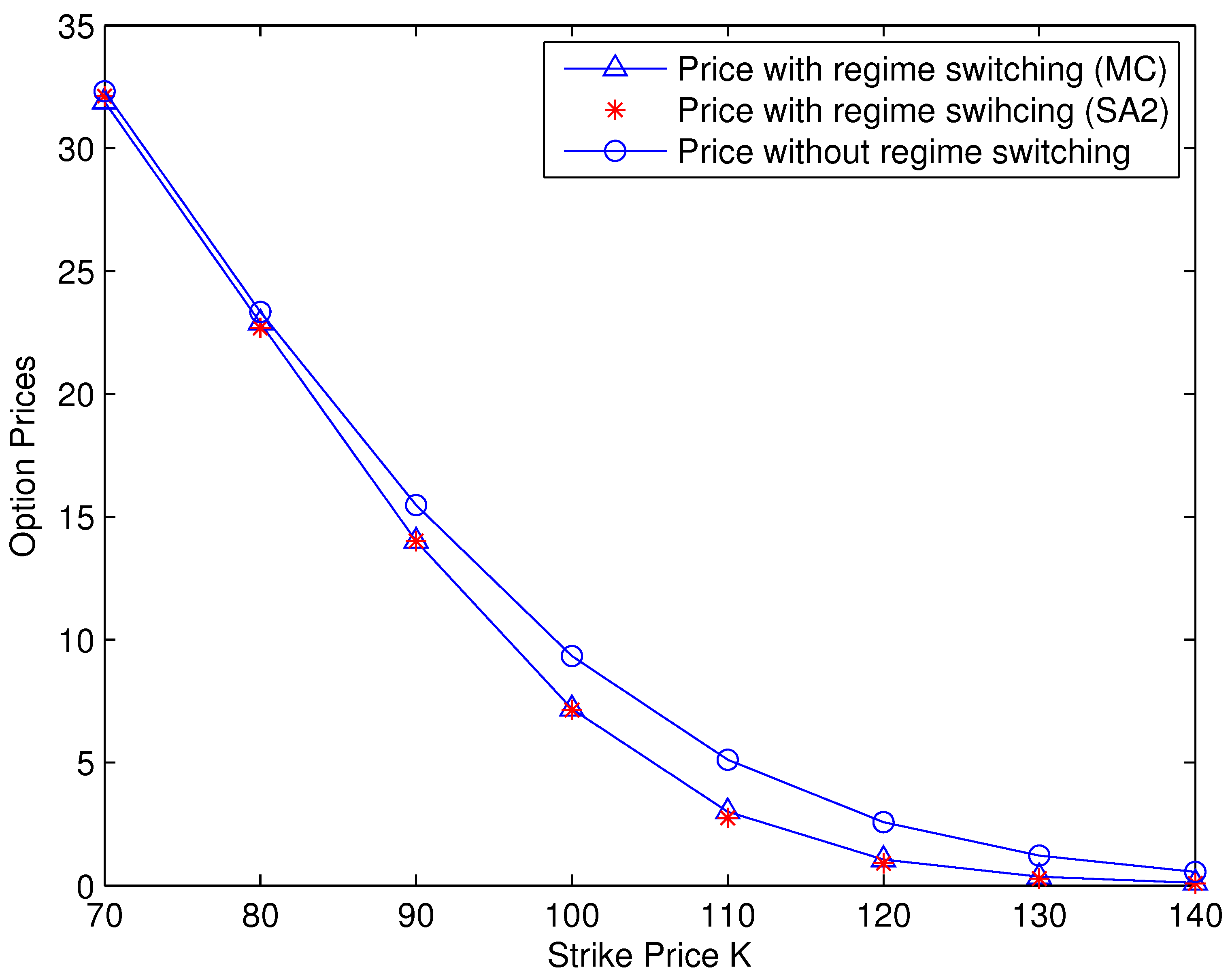
	with Regime-Switching	with Regime-Switching	without Regime-Switching
K	${\mathit{MC}}_{\mathbf{1}}$	$\mathit{SA}{\mathbf{2}}_{\mathbf{1}}$	First State
70	32.0532	32.1250	32.3157
80	22.8978	22.6910	23.3394
90	14.0194	14.0200	15.4829
100	7.1860	7.1398	9.3352
110	3.0066	2.7466	5.1183
120	1.0630	0.9057	2.5812
130	0.3573	0.2758	1.2193
140	0.1071	0.0829	0.1175

demonstrates option prices with different strikes under Markov-switching Heston’s stochastic volatility model as well as its non-switching Heston’s counterpart. In a non-switching Heston’s model, we assume all parameters’ value equals the parameters’ value in the first regime of the Markov-switching Heston’s model. The numerical results are shown in Figure 1 and it clearly shows that our approximation is quite precise. We also notice that the option prices calculated from the Markov-switching Heston’s model are cheaper than their non-switching counterparts over all range of strike prices given in the Table 2. This is because parameters’ value in a regime-switching Heston’s model is smaller. As ${\theta }_1<{\theta }_2$ and ${\mu }_1<{\mu }_2$, so $\frac{1}{T}\int {\theta }_{1}dt>\frac{1}{T}\int {\theta }_{t}dt$ and $\frac{1}{T}\int {\mu }_{1}dt>\frac{1}{T}\int \mu {}_{t}dt$. Figure 2 is the plot of the implied volatility. The maturity time is fixed at T = 1 and leaves other parameters unchanged. When $\rho$ is zero we get a volatility smile and the implied volatility starts to increase after the strike price is greater than the initial stock price. A negative $\rho$ has an obvious impact on the shape of the volatility curve: the volatility smile becomes a smirk. It seems that the changes in the initial regime only has an impact on the values of implied volatility, but not the shape of volatility curve.

6. Conclusions

This paper studies a saddlepoint approximation approach for pricing options in a Markov-switching Heston’s stochastic volatility model. Our approach requires to derive a closed-form expression of cumulant generating function, which needs to solve partial differential equations. The numerical results in Section 5 examine the accuracy of our method and a two-state case has been considered. The results show that saddlepoint method gives quite accuracy for the given range of maturities.

However, if the closed-form cumulant generating function does not exist, then one needs to rely on a numerical method to find a saddle point. In this situation, the procedure becomes slower.

In the future, it is worth considering multi-state Markov chain case and developing an algorithm to beat the curse of dimensionality. Furthermore, pricing American option under Markov-switching Heston’s stochastic volatility model and its calibration are interesting to study.

References

- Bollen, Nicolas P.B. 1998. Valuing options in regime-switching models. Journal of Derivatives 6: 38–49. [Google Scholar] [CrossRef]
- Boyle, Phelim, and Thangaraj Draviam. 2007. Pricing exotic options under regime switching. Insurance: Mathematics and Economics 40: 267–82. [Google Scholar] [CrossRef]
- Buffington, John, and Robert J. Elliott. 2002. American options with regime switching. International Journal of Theoretical and Applied Finance (IJTAF) 5: 497–514. [Google Scholar] [CrossRef]
- Chan, Leunglung, and Song-Ping Zhu. 2015. An explicit analytic formula for pricing barrier options with regime switching. Mathematics and Financial Economics 9: 29–37. [Google Scholar] [CrossRef]
- Chan, Leunglung, and Song-Ping Zhu. 2021a. An Analytic Approach for Pricing American Options with Regime Switching. Journal of Risk and Financial Management 14: 188. [Google Scholar] [CrossRef]
- Chan, Leunglung, and Song-Ping Zhu. 2021b. An Exact and Explicit Formula for Pricing Lookback Options with Regime Switching. Journal of Industrial and Management Optimization. [Google Scholar] [CrossRef]
- Daniels, Henry E. 1954. Saddleppoint Approximations in Statistics. Annals of Mathematical Statistics 25: 1943–78. [Google Scholar] [CrossRef]
- Daniels, Henry. E. 1987. Tail probability approximations. International Statistical Review 55: 37–48. [Google Scholar] [CrossRef]
- Duan, Jin-Chuan, Peter Ritchken, and Ivilina Popova. 2002. Option pricing under regime switching. Quantitative Finance 2: 116–32. [Google Scholar] [CrossRef]
- Elliott, Robert J., and Guang-Hua Lian. 2013. Pricing variance and volatility swaps in a stochastic volatility model with regime switching: Discrete observations case. Quantitative Finance 13: 687–98. [Google Scholar] [CrossRef]
- Elliott, Robert J., Lakhdar Aggoun, and John B. Moore. 1994. Hidden Markov Models: Estimation and Control. Berlin, Heidelberg and New York: Springer. [Google Scholar]
- Elliott, Robert J., Leunglung Chan, and Tak K. Siu. 2005. Option pricing and Esscher transform under regime switching. Annals of Finance 1: 423–32. [Google Scholar] [CrossRef]
- Elliott, Robert J., Leunglung Chan, and Tak K. Siu. 2013. Option valuation under a regime-switching constant elasticity of variance process. Applied Mathematics and Computation 219: 4434–43. [Google Scholar] [CrossRef]
- Elliott, Robert J., Tak K. Siu, and Leunglung Chan. 2014. On pricing barrier options with regime switching. Journal of Computational and Applied Mathematics 9: 196–210. [Google Scholar] [CrossRef]
- Egami, Masahiko, and Rusudan Kevkhishvili. 2020. A direct solution method for pricing options in regime-switching models. Mathematical Finance 30: 547–76. [Google Scholar] [CrossRef]
- Glasserman, Paul, and Kyoung-Kuk Kim. 2009. Saddlepoint Approximations for Affine Jump-Diffusion Models. Journal of Economic Dynamics and Control 33: 15–36. [Google Scholar] [CrossRef]
- Guo, Xin. 2001. Information and option pricings. Quantitative Finance 1: 38–44. [Google Scholar] [CrossRef]
- Hardy, Mary. 2001. A regime switching model of long-term stock returns. North American Actuarial Journal 5: 41–53. [Google Scholar] [CrossRef]
- Heston, Steven L. 1993. A closed-form solution for options with stochastic volatility with applications to bond and currency options. The Review of Financial Studies 6: 327–43. [Google Scholar] [CrossRef]
- Li, Jonathan Y., Michael J. Kim, and Roy H. Kwon. 2012. A moment approach to bounding exotic options under regime switching. Optimization 61: 1253–69. [Google Scholar] [CrossRef]
- Lu, Xiaoping, and Endah R. M. Putri. 2020. A semi-analytical valuation of American options under a two-state regime-switching economy. Physica A 538: 122968. [Google Scholar] [CrossRef]
- Vo, Minh T. 2009. Regime-switching stochastic volatility: Evidence from the crude oil market. Energy Economics 31: 779–88. [Google Scholar] [CrossRef]
- Zhang, Mengzhe, and Leunglung Chan. 2016. Saddlepoint Approximations to Option Price in a Regime-Switching Model. Annals of Finance 12: 55–69. [Google Scholar] [CrossRef]
- Zhu, Song-Ping, Alexander Badran, and Xiaoping Lu. 2012. A new exact solution for pricing European options in a two-state regime-switching economy. Computers and Mathematics with Applications 64: 2744–55. [Google Scholar] [CrossRef] [Green Version]