Self-Weighted LSE and Residual-Based QMLE of ARMA-GARCH Models ^†

Abstract

This paper studies the self-weighted least squares estimator (SWLSE) of the ARMA model with GARCH noises. It is shown that the SWLSE is consistent and asymptotically normal when the GARCH noise does not have a finite fourth moment. Using the residuals from the estimated ARMA model, it is shown that the residual-based quasi-maximum likelihood estimator (QMLE) for the GARCH model is consistent and asymptotically normal, but if the innovations are asymmetric, it is not as efficient as that when the GARCH process is observed. Using the SWLSE and residual-based QMLE as the initial estimators, the local QMLE for ARMA-GARCH model is asymptotically normal via an one-step iteration. The importance of the proposed estimators is illustrated by simulated data and five real examples in financial markets.

1. Introduction

Time series models have been extensively applied in various areas and many methodologies were proposed in the literature; for example, Zhang (2003) proposed a hybrid methodology that combines both ARIMA and ANN models to improve forecasting accuracy. Since Engle (1982), the ARCH-type models have been widely used in economics and finance. In particular, the GARCH model proposed by Bollerslev (1986) has been a benchmark in the risk management. Zhang and Zhang (2020) showed that the GARCH-based option-pricing models are able to price the SPX one-month variance swap rate, that is, the CBOE Volatility Index (VIX) accurately. Setiawan et al. (2021) used the GARCH($1,1$) model to analyze stock market turmoil during COVID-19 outbreak in an emerging and developed Economy.

However, recent research showed that the usual statistical inference procedure does not work if the fourth moment of the GARCH process does not exist. To make it clear, let us consider the AR(1)-GARCH($1,1$) model

$$y_t={\varphi }_1{y}_{t-1}+{\epsilon }_t,$$

(1)

$${\epsilon }_t={\eta }_t\sqrt{h_t}\mathrm{and}{h}_t={\alpha }_0+{\alpha }_1{\epsilon }_{t-1}^2+{\beta }_1{h}_{t-1},$$

(2)

where ${\alpha }_0>0$, ${\alpha }_1\ge 0$, ${\beta }_1\ge 0$, and ${\eta }_t$ is a sequence of independent and identically distributed (i.i.d.) innovations with zero mean and unit variance. For model (1), the least squares estimator (LSE) of ${\varphi }_1$ is

$${\widehat{\varphi }}_{LSn}\equiv {\left(\frac{1}{n}\sum _{t=1}^n{y}_{t-1}^2\right)}^{-1}\left(\frac{1}{\sqrt{n}}\sum _{t=1}^n{y}_{t-1}{y}_t\right),$$

where n is the sample size. Weiss (1986) and Pantula (1989) showed that ${\widehat{\varphi }}_{LSn}$ is $\sqrt{n}$-consistent and asymptotically normal if $E{\epsilon }_t^4<\infty$. However, $E{\epsilon }_t^4=\infty$ when the tail index $\alpha$ of ${\epsilon }_t$ is in $(0,4]$. In this case, Davis and Mikosch (1998) and Basrak et al. (2002) showed that ${\epsilon }_t$ has a heavy-tailed feature and its sample autocorrelation function is neither $\sqrt{n}$-consistent nor asymptotically normal. Lange (2011) showed that ${\widehat{\varphi }}_{LSn}$ is $n^{1-2/\alpha }$-consistent and converges to a stable random variable when $\alpha \in (2,4)$. Furthermore, for the AR model with ${\epsilon }_t$ being G-GARCH($1,1$) noise in He and Teräsvirta (1999), Zhang and Ling (2015) showed that

$$\frac{\sqrt{n}}{logn}({\widehat{\varphi }}_{LSn}-{\varphi }_1){⟶}_{\mathcal{L}}\mathrm{Normal},\mathrm{if}\alpha =4(\mathrm{i.e.}E{\epsilon }_t^4=\infty ),$$

(3)

$$n^{1-\frac{2}{\alpha }}({\widehat{\varphi }}_{LSn}-{\varphi }_1){⟶}_{\mathcal{L}}\mathrm{Stable},\mathrm{if}\alpha \in (2,4)(\mathrm{i.e.}E{\epsilon }_t^2<\infty \mathrm{and}E{\epsilon }_t^4=\infty ),$$

(4)

$$logn({\widehat{\varphi }}_{LSn}-{\varphi }_1){⟶}_{\mathcal{L}}\mathrm{Stable},\mathrm{if}\alpha =2(\mathrm{i.e.}E{\epsilon }_t^2=\infty ),$$

(5)

$${\widehat{\varphi }}_{LSn}-{\varphi }_1{⟶}_{\mathcal{L}}\mathrm{Stable},\mathrm{if}\alpha \in (0,2)(\mathrm{i.e.}E{\epsilon }_t^2=\infty ),$$

(6)

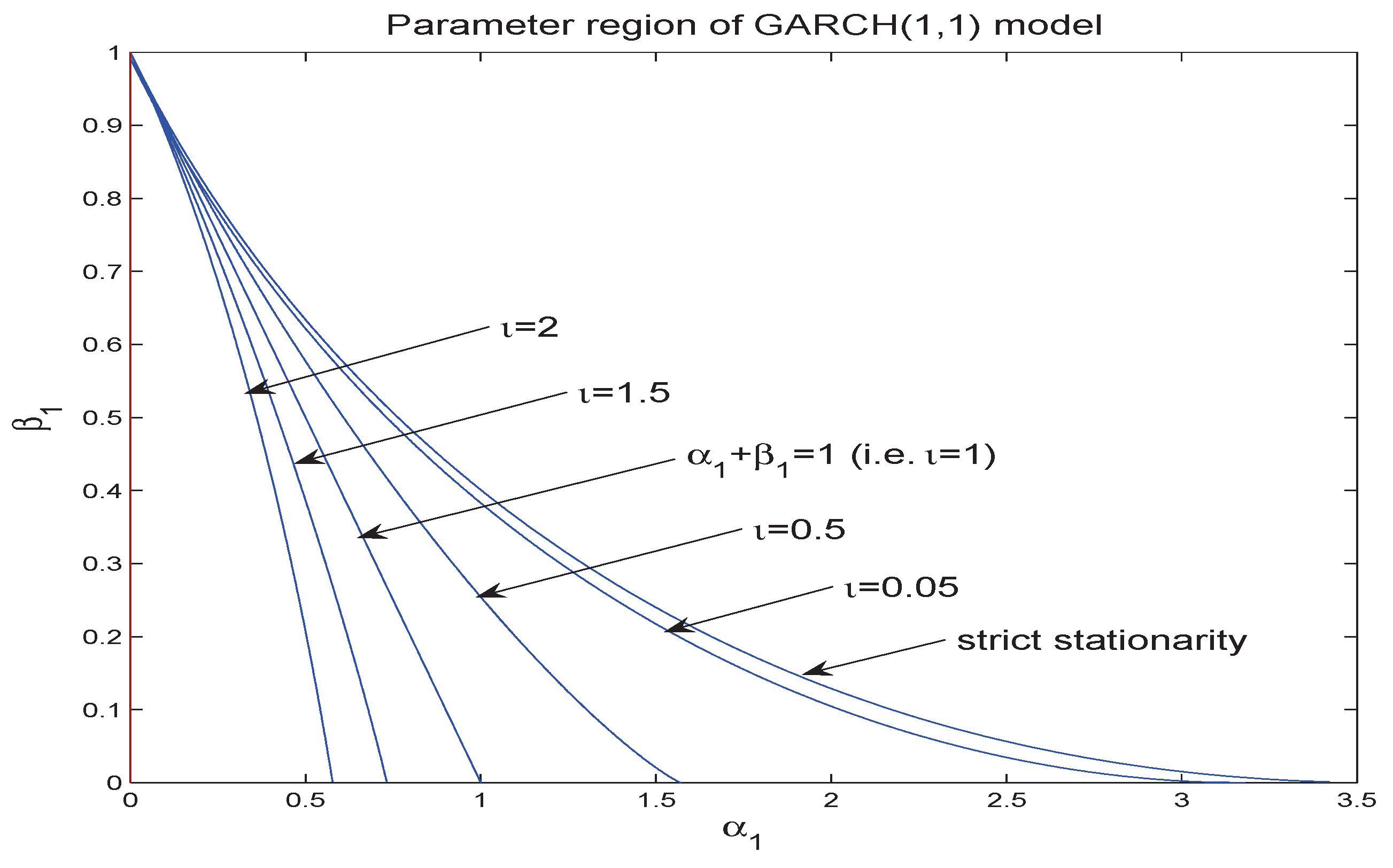
when $n\to \infty$, where ${⟶}_{\mathcal{L}}$ denotes the convergence in distribution. From (3)–(6), we find that the LSE not only has a slower rate of convergence but also is not asymptotically normal when $\alpha \in (0,4)$. Thus, based on the LSE, the classical theory and methodology (e.g., t-test, Wald test, and Ljung-Box test, among others) do not work in this case. Using a simulation method, we give the regime of parameter vector $({\alpha }_1,{\beta }_1)$ with $E{\epsilon }_t^{2\iota }<\infty$ in Figure 1 when ${\eta }_t\sim N(0,1)$. It can be seen that the regime of $({\alpha }_1,{\beta }_1)$ is very small for $E{\epsilon }_t^4<\infty$ (i.e., $\alpha >4$). In practice, the estimated value of $({\alpha }_1,{\beta }_1)$ does not lie in this regime, usually. Thus, it is very important to study the statistical inference when $\alpha \in (0,4]$. Zhu and Ling (2015) studied the self-weighted least absolute deviation estimator (SLADE) of the ARMA-GARCH model and showed that it is consistent and asymptotically normal when $\alpha \in (0,4]$.

This paper studies the self-weighted LSE (SWLSE) of the ARMA model with GARCH noises. It is shown that the SWLSE is consistent and asymptotically normal when the GARCH noise does not have a finite fourth moment (i.e., $\alpha \in (2,4]$). Using the residuals from the estimated ARMA model, it is shown that the residual-based quasi-maximum likelihood estimator (QMLE) for the GARCH model is consistent and asymptotically normal, but if the innovations are asymmetric, it is not as efficient as that when the GARCH process is observed. Using the SWLSE and residual-based QMLE as the initial estimators, the local QMLE for ARMA-GARCH model is asymptotically normal via an one-step iteration.

This paper is arranged as follows. Section 2 presents the model and assumptions. Section 3 presents our main results. Section 4 presents simulation results and Section 5 gives real examples. All the proofs are deferred into the Appendix A.

2. Model and Assumptions

Assume that $\{y_t:t=0,\pm 1,\pm 2,\cdots \}$ are generated by the ARMA-GARCH model

$$y_t=\mu +\sum _{i=1}^p{\varphi }_i{y}_{t-i}+\sum _{i=1}^q{\psi }_i{\epsilon }_{t-i}+{\epsilon }_t,$$

(7)

$${\epsilon }_t={\eta }_t\sqrt{h_t}\mathrm{and}{h}_t={\alpha }_0+\sum _{i=1}^r{\alpha }_i{\epsilon }_{t-i}^2+\sum _{i=1}^s{\beta }_i{h}_{t-i},$$

(8)

where ${\alpha }_i\ge 0$ and ${\beta }_j\ge 0$, $i=0,\cdots ,r$, $j=1,\cdots ,s$, and ${\eta }_t$ is defined as in (2). Denote $\gamma ={(\mu ,{\varphi }_1,\cdots ,{\varphi }_p,{\psi }_1,\cdots ,{\psi }_q)}^{\prime }$, $\delta ={({\alpha }_0,{\alpha }_1,\cdots ,{\alpha }_r,{\beta }_1,\cdots ,{\beta }_s)}^{\prime }$, and $\lambda ={({\gamma }^{\prime },{\delta }^{\prime })}^{\prime }$. Let ${\gamma }_0$, ${\delta }_0$, and ${\theta }_0$ be the true values of $\gamma$, $\delta$, and $\theta$, respectively. The parameter subspaces ${\Theta }_{\gamma }\subset R^{p+q+1}$ and ${\Theta }_{\delta }\subset R_0^{r+s+1}$ are compact, where $R=(-\infty ,\infty )$ and $R_0=[0,\infty )$. Denote $\Theta ={\Theta }_{\gamma }\times {\Theta }_{\delta }$, $m=p+q+r+s+2$, $\alpha \left(z\right)={\sum }_{i=1}^r{\alpha }_i{z}^i$, $\beta \left(z\right)=1-{\sum }_{i=1}^s{\beta }_i{z}^i$, $\varphi \left(z\right)=1-{\sum }_{i=1}^p{\varphi }_i{z}^i$, and $\psi \left(z\right)=1+{\sum }_{i=1}^q{\psi }_i{z}^i$. We introduce the following conditions:

Assumption 1.

${\theta }_0$ is an interior point in Θ and for each $\theta \in \Theta$, $\varphi \left(z\right)\ne 0$ and $\psi \left(z\right)\ne 0$ when $\left|z\right|\le 1$, and $\varphi \left(z\right)$ and $\psi \left(z\right)$ have no common root with ${\varphi }_p\ne 0$ or ${\psi }_q\ne 0$.

Assumption 2.

$\alpha \left(z\right)$ and $\beta \left(z\right)$ have no common root, ${\alpha }_r+{\beta }_s\ne 0$, and ${\sum }_{i=1}^r{\alpha }_i+{\sum }_{j=1}^s{\beta }_j<1$ for each $\theta \in \Theta$.

Assumption 1 is the stationarity and invertibility condition of ARMA models, under which it follows that

$${\psi }^{-1}\left(z\right)=\sum _{i=0}^{\infty }{a}_{\psi }\left(i\right)z^i\mathrm{and}\varphi \left(z\right){\psi }^{-1}\left(z\right)=\sum _{i=0}^{\infty }{a}_{\gamma }\left(i\right)z^i,$$

(9)

where ${\sup }_{{\Theta }_{\gamma }}\left|a_{\psi }\left(i\right)\right|=O\left({\rho }^i\right)$ and ${\sup }_{{\Theta }_{\gamma }}\left|a_{\gamma }\left(i\right)\right|=O\left({\rho }^i\right)$ with $\rho \in (0,1)$. Assumption 2 ensures that $\left\{{\epsilon }_t\right\}$ is strictly stationary and ergodic with $E{\epsilon }_t^2<\infty$, see Ling and Li (1997) and Ling and McAleer (2002). It is also the identifiability condition for model (2) and, by Lemma 2.1 in Ling (1999), the condition ${\sum }_{i=1}^s{\beta }_i<1$ is equivalent to

$$\begin{array}{c}\hfill 0\le \rho \left(G\right)<1,\mathrm{where}G=\left(\begin{array}{ccc}{\beta }_1& \cdots & {\beta }_s\\ I_{s-1}& & O\end{array}\right),\end{array}$$

(10)

$I_k$ is the $k\times k$ identity matrix, and $\rho \left(B\right)$ is the spectral radius of matrix B. Under this condition, we have

$$\begin{array}{c}\hfill {\beta }^{-1}\left(z\right)=\sum _{i=0}^{\infty }{a}_{\beta }\left(i\right)z^i\mathrm{and}\alpha \left(z\right){\beta }^{-1}\left(z\right)=\sum _{i=1}^{\infty }{a}_{\delta }\left(i\right)z^i,\end{array}$$

(11)

where ${\sup }_{{\Theta }_{\delta }}\left|a_{\beta }\left(i\right)\right|=O\left({\rho }^i\right)$ and ${\sup }_{{\Theta }_{\delta }}\left|a_{\delta }\left(i\right)\right|=O\left({\rho }^i\right)$ with $\rho =\rho \left(G\right)$.

Given the observations $\{y_n,$$\cdots ,y_1\}$ and initial value $Y_0\equiv \{y_0,y_{-1},\cdots \}$, we can write the parametric model as

$${\epsilon }_t\left(\gamma \right)=y_t-\mu -\sum _{i=1}^p{\varphi }_i{y}_{t-i}-\sum _{i=1}^q{\psi }_i{\epsilon }_{t-i}\left(\gamma \right),$$

(12)

$${\eta }_t\left(\lambda \right)={\epsilon }_t\left(\gamma \right)/\sqrt{h_t\left(\lambda \right)}\mathrm{and}{h}_t\left(\lambda \right)={\alpha }_0+\sum _{i=1}^r{\alpha }_i{\epsilon }_{t-i}^2\left(\gamma \right)+\sum _{i=1}^s{\beta }_i{h}_{t-i}\left(\lambda \right).$$

(13)

It is easy to see that ${\eta }_t\left({\lambda }_0\right)={\eta }_t$, ${\epsilon }_t\left({\gamma }_0\right)={\epsilon }_t$, and $h_t\left({\lambda }_0\right)=h_t$. In practice, we do not observe those $y_i$ in $Y_0$ and hence they have to be replaced by some constants. This does not affect our asymptotic results, see Ling and McAleer (2003a). For simplicity, we do not study this case in details.

3. Main Results

The self-weighted estimation approach was proposed by Ling (2005) and it has been used to solve the problem on statistical inference of the heavy-tailed ARMA-GARCH model in Ling (2007) and Zhu and Ling (2011). Using a similar idea, we define the SWLSE as

$${\tilde{\gamma }}_n=arg\underset{\gamma \in {\Theta }_{\gamma }}{min}\sum _{t=1}^n\frac{{\epsilon }_t^2\left(\gamma \right)}{w_t},$$

where $w_t=1+{\sum }_{k=1}^{\infty }{k}^{-1/2-1}\left|y_{t-k}\right|$. We can state the following result:

Theorem 1.

Suppose that Assumptions 1 and 2 hold. Then, as $n\to \infty$,

$$\left(i\right){\tilde{\gamma }}_n{⟶}_p{\gamma }_0,$$

$$\left(ii\right)\sqrt{n}({\tilde{\gamma }}_n-{\gamma }_0){⟶}_{\mathcal{L}}N(0,A^{-1}B{A}^{-1}),$$

where ${⟶}_p$ denotes the convergence in probability, $A=E\left(w_t^{-1}{M}_t\right)$, $B=E\left(w_t^{-2}{h}_t{M}_t\right)$, and $M_t=[\partial {\epsilon }_t\left({\gamma }_0\right)/\partial \gamma ]{[\partial {\epsilon }_t\left({\gamma }_0\right)/\partial \gamma ]}^{\prime }$.

The preceding result holds for any kind of ARCH-type errors only if $E{h}_t<\infty$, see the proof in the Appendix A. To easily understand it, we refer to model (1) and (2) again. In this case, the information function is $E(y_{t-1}^2/w_t)\le E\left|y_{t-1}\right|<\infty$. The score function is $n^{-1/2}{\sum }_{t=1}^n{y}_{t-1}{\epsilon }_t/w_t$ and $E{(y_{t-1}{\epsilon }_t/w_t)}^2\le O\left(1\right)E{h}_t<\infty$, which is the condition we need for the GARCH errors. This result holds when $E{\epsilon }_t^4<\infty$, but it is not as efficient as the LSE in this case. When $E{\epsilon }_t^4=\infty$ and $E{\epsilon }_t^2<\infty$, the process $y_t$ has a heavy tailed feature and the SWLSE has a faster rate of convergence than that of LSE. The weight function $w_t$ can be replaced by others, see Ling (2007).

Next, we use the residual ${\tilde{\epsilon }}_t\equiv {\epsilon }_t\left({\tilde{\gamma }}_n\right)$ from ARMA parts as the artificial observation of ${\epsilon }_t$. The log-quasi-likelihood function based on ${\tilde{\epsilon }}_t$ can be written as

$$\begin{array}{c}\hfill {\tilde{L}}_{\delta n}\left(\delta \right)=\frac{1}{n}\sum _{t=1}^n{\tilde{l}}_t\left(\delta \right)\mathrm{and}{\tilde{l}}_t\left(\delta \right)=-\frac{1}{2}log{\tilde{h}}_t\left(\delta \right)-\frac{{\tilde{\epsilon }}_t^2}{2{\tilde{h}}_t\left(\delta \right)},\end{array}$$

(14)

where ${\tilde{h}}_t\left(\delta \right)=h_t{\left(\lambda \right)|}_{\gamma ={\tilde{\gamma }}_n}$. We define the residual-based QMLE of ${\delta }_0$ as

$${\tilde{\delta }}_n=arg\underset{\delta \in {\Theta }_{\delta }}{max}{\tilde{L}}_{\delta n}\left(\delta \right).$$

Denote $H_{\delta t}\left(\lambda \right)=h_t^{-2}\left(\lambda \right)[\partial h_t\left(\lambda \right)/\partial \delta ][\partial h_t\left(\lambda \right)/\partial {\delta }^{\prime }]$ and $H_{\delta t}\left({\lambda }_0\right)$ by $H_{\delta t}$. We now give the asymptotic properties of ${\tilde{\delta }}_n$ as follows.

Theorem 2.

Suppose that Assumptions 1 and 2 hold. Then, as $n\to \infty$,

$$\begin{array}{ccc}\hfill \left(i\right)& & {\tilde{\delta }}_n{⟶}_p{\delta }_0,\mathrm{if}E{\left|{\eta }_t\right|}^{2+\tilde{\iota }}<\infty \mathit{for}\mathit{some}\tilde{\iota }>0,\hfill \\ \hfill \left(ii\right)& & \sqrt{n}({\tilde{\delta }}_n-{\delta }_0){⟶}_{\mathcal{L}}N(0,{\left(E{H}_{\delta t}\right)}^{-1}{\Omega }_{\delta }{\left(E{H}_{\delta t}\right)}^{-1}),\mathrm{if}E{\eta }_t^4<\infty ,\hfill \end{array}$$

where ${\Omega }_{\delta }=\kappa E{H}_{\delta t}+E{D}_t\left(A^{-1}B{A}^{-1}\right)E{D}_t^{\prime }+{\kappa }_3{\tilde{\Omega }}_{\delta }$, ${\tilde{\Omega }}_{\delta }=E{D}_t{A}^{-1}E\left(w_t^{-1}{\tilde{D}}_t^{\prime }\right)$$+E\left(w_t^{-1}{\tilde{D}}_t\right)A^{-1}E{D}_t^{\prime }$, $\kappa =E{\eta }_t^4-1$, ${\kappa }_3=E{\eta }_t^3$, $D_t=E\left\{h_t^{-2}[\partial h_t\left({\lambda }_0\right)/\partial \delta ][\partial h_t\left({\lambda }_0\right)/\partial {\gamma }^{\prime }]\right\}$, and ${\tilde{D}}_t=E\left\{h_t^{-1/2}[\partial h_t\left({\lambda }_0\right)/\partial \delta ][\partial {\epsilon }_t\left({\gamma }_0\right)/\partial {\gamma }^{\prime }]\right\}$.

When ${\eta }_t$ is symmetric and $\mu =0$, we have $E{\eta }_t^3=0$, $E{D}_t=E{\tilde{D}}_t=0$, and hence ${\Omega }_{\delta }=\kappa E{H}_{\delta t}$. When the conditional mean is zero (i.e., $y_t={\epsilon }_t$), model (7) and (8) reduces to the GARCH model. In this case, the log-quasi-likelihood function based on ${\epsilon }_t$ can be written as

$$\begin{array}{c}\hfill L_{\delta n}\left(\delta \right)=\frac{1}{n}\sum _{t=1}^n{l}_t\left(\delta \right)\mathrm{and}{l}_t\left(\delta \right)=-\frac{1}{2}log{h}_t\left(\delta \right)-\frac{{\epsilon }_t^2}{2h_t\left(\delta \right)}.\end{array}$$

(15)

Then, the global QMLE of ${\delta }_0$ is defined as ${\overline{\delta }}_n=arg{\max }_{\delta \in {\Theta }_{\delta }}{L}_{\delta n}\left(\delta \right)$. Berkes et al (2003) and Hall and Yao (2003) showed that ${\overline{\delta }}_n$ is consistent and as $n\to \infty$,

$$\begin{array}{c}\hfill \sqrt{n}({\overline{\delta }}_n-{\delta }_0){⟶}_{\mathcal{L}}N(0,\kappa {\left(E{H}_{\delta t}\right)}^{-1}),\mathrm{if}E{\eta }_t^4<\infty .\end{array}$$

(16)

From Theorem 2, we see that the efficiency of the estimated ${\delta }_0$ is affected by the estimated parameters in ARMA parts unless ${\eta }_t$ has a symmetric density and $\mu$ is known to be zero without estimation. This gives a reminder to practitioners that we need to be careful when ones use the residuals to estimate the GARCH model.

Given $\{y_n,\cdots ,y_1\}$ and the initial value $Y_0$, we can write down the log-quasi-likelihood function of model (7) and (8) as follows:

$$\begin{array}{c}\hfill L_n\left(\lambda \right)=\frac{1}{n}\sum _{t=1}^n{l}_t\left(\lambda \right)\mathrm{and}{l}_t\left(\lambda \right)=-\frac{1}{2}log{h}_t\left(\lambda \right)-\frac{{\epsilon }_t^2\left(\gamma \right)}{2h_t\left(\lambda \right)}.\end{array}$$

(17)

Then, the global QMLE of ${\lambda }_0$ is defined as the maximizer of $L_n\left(\lambda \right)$ in $\Theta$. Ling and McAleer (2003a) proved the consistency of this QMLE. But the asymptotic normality of this QMLE requires $E{\epsilon }_t^4<\infty$, see also Francq and Zakoïan (2004).

Based on ${\tilde{\lambda }}_n\equiv {({\tilde{\gamma }}_n^{\prime },{\tilde{\delta }}_n^{\prime })}^{\prime }$, we obtain the local QMLE through an one-step iteration

$$\begin{array}{c}\hfill {\widehat{\lambda }}_n={\tilde{\lambda }}_n-{\left[\sum _{t=1}^n\frac{{\partial }^2{l}_t\left({\tilde{\lambda }}_n\right)}{\partial \lambda \partial {\lambda }^{\prime }}\right]}^{-1}\sum _{t=1}^n\frac{\partial l_t\left({\tilde{\lambda }}_n\right)}{\partial \lambda }.\end{array}$$

(18)

As in Ling (2007), we can show that as $n\to \infty$,

$$\begin{array}{c}\hfill \sqrt{n}({\widehat{\lambda }}_n-{\lambda }_0){⟶}_{\mathcal{L}}N(0,{\Sigma }^{-1}\Omega {\Sigma }^{-1}),\end{array}$$

where $\Sigma =E\left[U_t\left({\lambda }_0\right)U_t^{\prime }\left({\lambda }_0\right)\right]$, $\Omega =E\left[U_t\left({\lambda }_0\right)J{U}_t^{\prime }\left({\lambda }_0\right)\right]$, $J=\left(\begin{array}{cc}1& {\kappa }_3\\ {\kappa }_3& \kappa \end{array}\right)$, and $U_t\left(\lambda \right)=[h_t^{-1/2}\partial {\epsilon }_t\left(\gamma \right)/\partial \lambda ,h_t^{-1}\partial h_t\left(\lambda \right)/\partial \lambda ]$. When ${\eta }_t\sim N(0,1)$, the local QMLE is efficient. So, Theorems 1 and 2 provide an approach to obtain an efficient estimator for the full ARMA-GARCH models under the finite second moment condition of ${\epsilon }_t$. When ${\eta }_t$ is not normal, the efficient and adaptive estimators can be obtained by using the results in this section and following the similar lines as in Drost et al. (1997), Drost and Klaassen (1997), Ling (2003), and Ling and McAleer (2003b).

4. Simulation Study

In this section, we assess the finite sample performance of ${\tilde{\lambda }}_n={({\tilde{\gamma }}_n^{\prime },{\tilde{\delta }}_n^{\prime })}^{\prime }$ and ${\widehat{\lambda }}_n={({\widehat{\gamma }}_n^{\prime },{\widehat{\delta }}_n^{\prime })}^{\prime }$, where ${\tilde{\gamma }}_n$ is the SWLSE, ${\tilde{\delta }}_n$ is the residual-based QMLE, and ${\widehat{\lambda }}_n$ is the local QMLE. We generate 1000 replications of sample size $n=1000$ and 2000 from the following model

$$y_t={\varphi }_{10}{y}_{t-1}+{\psi }_{10}{\epsilon }_{t-1}+{\epsilon }_t,$$

(19)

$${\epsilon }_t={\eta }_t\sqrt{h_t}\mathrm{and}{h}_t={\alpha }_{00}+{\alpha }_{10}{\epsilon }_{t-1}^2+{\beta }_{10}{h}_{t-1},$$

(20)

where ${\gamma }_0^{\prime }=({\varphi }_{10},{\psi }_{10})=(0.4,0.5)$, ${\delta }_0^{\prime }=({\alpha }_{00},{\alpha }_{10},{\beta }_{10})=(0.1,0.1,0.8)$, and ${\eta }_t$ is chosen to be the standard normal N($0,1$) distribution, re-scaled Laplace $L(0,1)$ distribution, or re-scaled student’s $t\left(5\right)$ distribution with $E{\eta }_t^2=1$.

Table 1. The results of ${\tilde{\lambda }}_n$ and ${\widehat{\lambda }}_n$.

			${\tilde{\mathit{\lambda }}}_{\mathit{n}}$
${\eta }_t$	n		${\tilde{\varphi }}_{1n}$	${\tilde{\psi }}_{1n}$	${\tilde{\alpha }}_{0n}$	${\tilde{\alpha }}_{1n}$	${\tilde{\beta }}_{1n}$
$N(0,1)$	1000	Bias	−0.0012	0.0032	0.0189	0.0012	−0.0235
		SD	0.0443	0.0423	0.0650	0.0278	0.0839
		AD	0.0424	0.0402	0.0524	0.0290	0.0726
	2000	Bias	−0.0017	0.0015	0.0083	−0.0000	−0.0103
		SD	0.0300	0.0293	0.0342	0.0204	0.0471
		AD	0.0300	0.0285	0.0332	0.0201	0.0469
			${\widehat{\lambda }}_n$
			${\widehat{\varphi }}_{1n}$	${\widehat{\psi }}_{1n}$	${\widehat{\alpha }}_{0n}$	${\widehat{\alpha }}_{1n}$	${\widehat{\beta }}_{1n}$
	1000	Bias	−0.0010	0.0022	0.0172	0.0015	−0.0210
		SD	0.0425	0.0406	0.0657	0.0282	0.0845
		AD	0.0405	0.0380	0.0526	0.0291	0.0729
	2000	Bias	−0.0016	0.0012	0.0073	−0.0000	−0.0087
		SD	0.0283	0.0274	0.0340	0.0205	0.0470
		AD	0.0286	0.0270	0.0332	0.0202	0.0469
			${\tilde{\lambda }}_n$
			${\tilde{\varphi }}_{1n}$	${\tilde{\psi }}_{1n}$	${\tilde{\alpha }}_{0n}$	${\tilde{\alpha }}_{1n}$	${\tilde{\beta }}_{1n}$
$L(0,1)$	1000	Bias	−0.0032	0.0035	0.0241	0.0020	−0.0304
		SD	0.0454	0.0414	0.0806	0.0381	0.1079
		AD	0.0456	0.0433	0.0639	0.0385	0.0909
	2000	Bias	−0.0001	0.0014	0.0116	0.0016	−0.0148
		SD	0.0328	0.0307	0.0426	0.0268	0.0599
		AD	0.0323	0.0307	0.0397	0.0269	0.0577
			${\widehat{\lambda }}_n$
			${\widehat{\varphi }}_{1n}$	${\widehat{\psi }}_{1n}$	${\widehat{\alpha }}_{0n}$	${\widehat{\alpha }}_{1n}$	${\widehat{\beta }}_{1n}$
	1000	Bias	−0.0027	0.0028	0.0237	0.0028	−0.0296
		SD	0.0444	0.0402	0.0918	0.0390	0.1183
		AD	0.0443	0.0416	0.0641	0.0387	0.0913
	2000	Bias	−0.0008	0.0013	0.0109	0.0019	−0.0138
		SD	0.0316	0.0296	0.0424	0.0270	0.0598
		AD	0.0313	0.0295	0.0397	0.0270	0.0578
			${\tilde{\lambda }}_n$
			${\tilde{\varphi }}_{1n}$	${\tilde{\psi }}_{1n}$	${\tilde{\alpha }}_{0n}$	${\tilde{\alpha }}_{1n}$	${\tilde{\beta }}_{1n}$
$t\left(5\right)$	1000	Bias	−0.0012	0.0016	0.0300	0.0046	−0.0395
		SD	0.0460	0.0445	0.0867	0.0432	0.1137
		AD	0.0454	0.0431	0.0734	0.0443	0.1038
	2000	Bias	0.0014	0.0005	0.0126	0.0025	−0.0164
		SD	0.0312	0.0305	0.0463	0.0325	0.0657
		AD	0.0323	0.0308	0.0459	0.0316	0.0666
			${\widehat{\lambda }}_n$
			${\widehat{\varphi }}_{1n}$	${\widehat{\psi }}_{1n}$	${\widehat{\alpha }}_{0n}$	${\widehat{\alpha }}_{1n}$	${\widehat{\beta }}_{1n}$
	1000	Bias	−0.0022	0.0018	0.0291	0.0054	−0.0381
		SD	0.0472	0.0448	0.0897	0.0444	0.1166
		AD	0.0443	0.0417	0.0737	0.0445	0.1042
	2000	Bias	0.0006	0.0007	0.0119	0.0030	−0.0155
		SD	0.0317	0.0296	0.0462	0.0330	0.0656
		AD	0.0315	0.0297	0.0459	0.0317	0.0667

reports the sample bias (Bias), the sample standard deviations (SD), and the average estimated asymptotic standard deviation (AD) of ${\tilde{\lambda }}_n$ and ${\widehat{\lambda }}_n$. From this table, we find that (i) each considered estimator has a small bias, and its value of SD is close to that of AD, demonstrating the validity of its asymptotic normality; (ii) ${\widehat{\gamma }}_n$ could be slightly more efficient than ${\tilde{\gamma }}_n$, whereas ${\widehat{\delta }}_n$ is as efficient as ${\tilde{\delta }}_n$; (iii) all estimators for ${\eta }_t\sim N(0,1)$ are more efficient than the corresponding ones for ${\eta }_t\sim L(0,1)$ or $t\left(5\right)$. All these findings are consistent with our theory in Section 3. We should mention that the QMLE of ${\delta }_0$ is not reliable when the sample size n is less than 800 according to our simulation experiments and hence the results are not reported here.

As a comparison, we compute the classical LSE ${\widehat{\gamma }}_{LSn}={({\widehat{\varphi }}_{LSn},{\widehat{\psi }}_{LSn})}^{\prime }$ for ${\gamma }_0$ in model (19) and (20), where ${\widehat{\gamma }}_{LSn}$ is computed in a similar way as ${\tilde{\gamma }}_n$ with $w_t\equiv 1$.

Table 2. The results of ${\widehat{\gamma }}_{LSn}$.

		${\mathit{\eta }}_{\mathit{t}}\sim \mathit{N}(0,1)$			${\mathit{\eta }}_{\mathit{t}}\sim \mathit{L}(0,1)$			${\mathit{\eta }}_{\mathit{t}}\sim \mathit{t}\left(5\right)$
n		${\widehat{\varphi }}_{LSn}$	${\widehat{\psi }}_{LSn}$		${\widehat{\varphi }}_{LSn}$	${\widehat{\psi }}_{LSn}$		${\widehat{\varphi }}_{LSn}$	${\widehat{\psi }}_{LSn}$
1000	Bias	0.0001	0.0012		−0.0034	0.0024		−0.0033	0.0015
	SD	0.0441	0.0412		0.0482	0.0473		0.0518	0.0487
	AD	0.0437	0.0411		0.0507	0.0474		0.0525	0.0490
2000	Bias	−0.0018	0.0015		−0.0009	0.0011		−0.0008	0.0010
	SD	0.0307	0.0299		0.0350	0.0325		0.0382	0.0349
	AD	0.0311	0.0293		0.0367	0.0344		0.0382	0.0358

reports the corresponding results of ${\widehat{\gamma }}_{LSn}$. Compared with ${\tilde{\gamma }}_n$ in Table 1, we find that ${\widehat{\gamma }}_{LSn}$ is less efficient than ${\tilde{\gamma }}_n$ for all examined cases. This finding suggests that it seems better to fit the ARMA model by the SWLSE rather than the LSE method when the data exhibit the conditionally heteroscedastic effect.

5. Real Examples

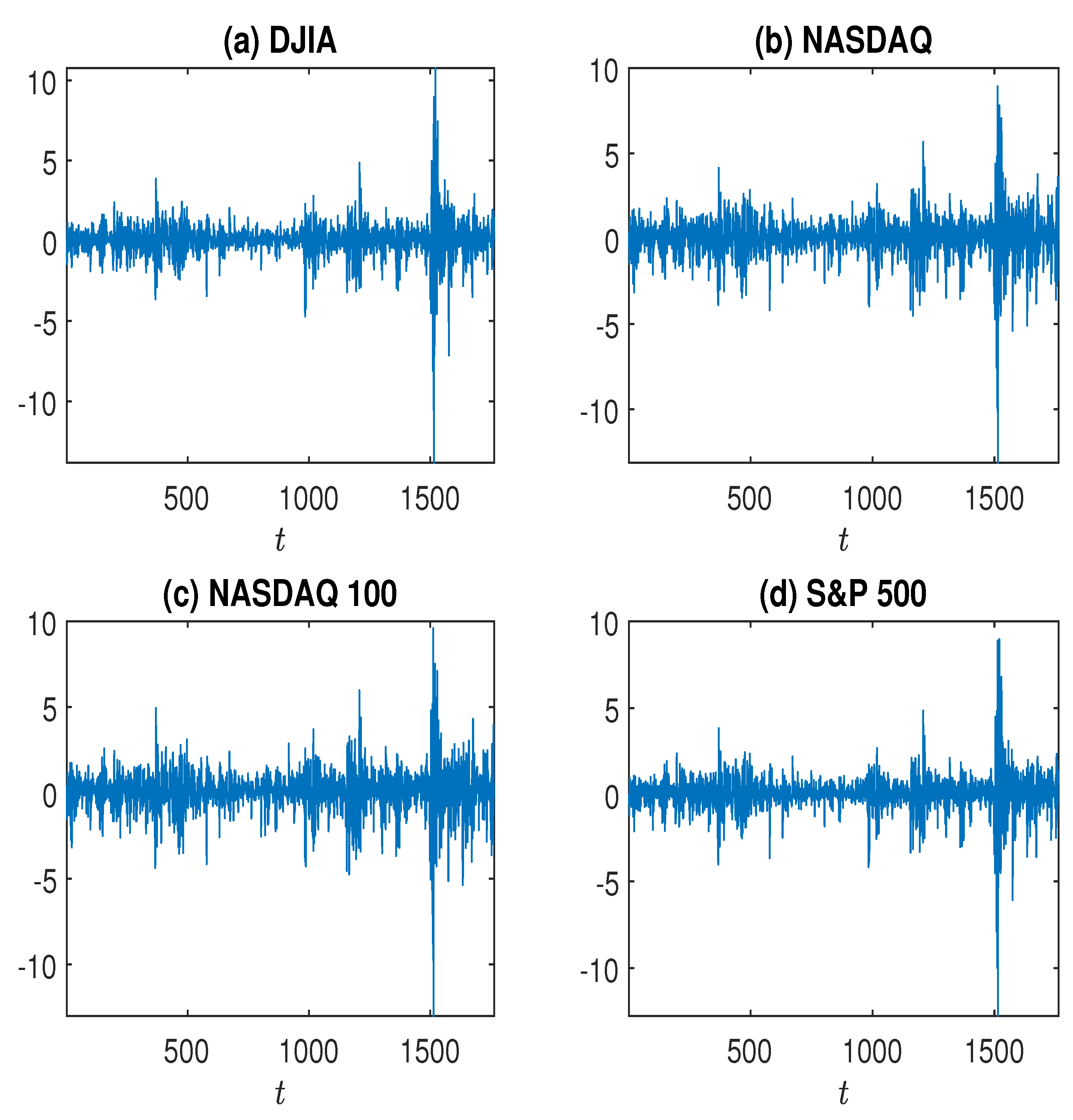
This section first studies the log returns ($\times 100$) of DJIA, NASDAQ, NASDAQ 100, and S&P 500 from 11 March 2015 to 10 March 2021, with a total of 1764 observations (see Figure 2). Denote each log return series by ${\left\{y_t\right\}}_{t=1}^{1764}$. Before fitting an AR(1)-GARCH($1,1$) to ${\left\{y_t\right\}}_{t=1}^{1764}$, we first estimate ${\alpha }_y$, the tail index of $|y_t|$, and get the following results:

$$\begin{array}{cc}\hfill \left(\mathrm{DJIA}\right)& {\widehat{\alpha }}_y=2.3029,\left(\mathrm{NASDAQ}\right){\widehat{\alpha }}_y=3.2592,\hfill \\ & \left(0.9285\right)\left(0.6830\right)\hfill \\ \hfill \left(\mathrm{NASDAQ}100\right)& {\widehat{\alpha }}_y=3.6956,\left(\mathrm{S}\&\mathrm{P}500\right){\widehat{\alpha }}_y=2.5329,\hfill \\ & \left(0.6077\right)\left(0.8567\right)\hfill \end{array}$$

where ${\widehat{\alpha }}_y$ is the proposed estimator of ${\alpha }_y$ in Hill (2010), and the value in parentheses is the AD of ${\widehat{\alpha }}_y$. From the above results, we can conclude that each $|y_t|$ has a finite second moment, but does not have a finite fourth moment. Hence, it is reasonable to fit four return series by using the procedure in Section 3, that is, we first obtain the SWLSE ${\tilde{\gamma }}_n$ and the residual-based QMLE ${\tilde{\delta }}_n$, and then obtain the local QMLE ${\widehat{\lambda }}_n$. The resulting fitted models are as follows:

$$\begin{array}{cc}\hfill \left(\mathrm{DJIA}\right)& \left\{\begin{array}{c}{y}_t=0.0859-0.0461y_{t-1}+{\epsilon }_t,\hfill \\ \left(0.0173\right)\left(0.0292\right)\hfill \\ h_t=0.0416+0.2108{\epsilon }_{t-1}^2+0.7532h_{t-1},\hfill \\ \left(0.0109\right)\left(0.0378\right)\left(0.0377\right)\hfill \end{array}\right.\hfill \\ \hfill \left(\mathrm{NASDAQ}\right)& \left\{\begin{array}{c}{y}_t=0.1009-0.0663y_{t-1}+{\epsilon }_t,\hfill \\ \left(0.0216\right)\left(0.0275\right)\hfill \\ h_t=0.0643+0.1747{\epsilon }_{t-1}^2+0.7826h_{t-1},\hfill \\ \left(0.0178\right)\left(0.0335\right)\left(0.0367\right)\hfill \end{array}\right.\hfill \\ \hfill \left(\mathrm{NASDAQ}100\right)& \left\{\begin{array}{c}{y}_t=0.1125-0.0654y_{t-1}+{\epsilon }_t,\hfill \\ \left(0.0225\right)\left(0.0276\right)\hfill \\ h_t=0.0668+0.1751{\epsilon }_{t-1}^2+0.7855h_{t-1},\hfill \\ \left(0.0180\right)\left(0.0325\right)\left(0.0351\right)\hfill \end{array}\right.\hfill \\ \hfill \left(\mathrm{S}\&\mathrm{P}500\right)& \left\{\begin{array}{c}{y}_t=0.0910-0.0838y_{t-1}+{\epsilon }_t,\hfill \\ \left(0.0171\right)\left(0.0289\right)\hfill \\ h_t=0.0432+0.2206{\epsilon }_{t-1}^2+0.7453h_{t-1},\hfill \\ \left(0.0117\right)\left(0.0422\right)\left(0.0414\right)\hfill \end{array}\right.\hfill \end{array}$$

where all estimated parameters are the local QMLE ${\widehat{\lambda }}_n$, and the values in parentheses are the ADs of ${\widehat{\lambda }}_n$. From these fitted models, we can find that all estimated parameters are significantly different from zero at the level of 5%. In particular, the significant parameters in the fitted AR models imply that the U.S. stock market is not efficient during the examined period.

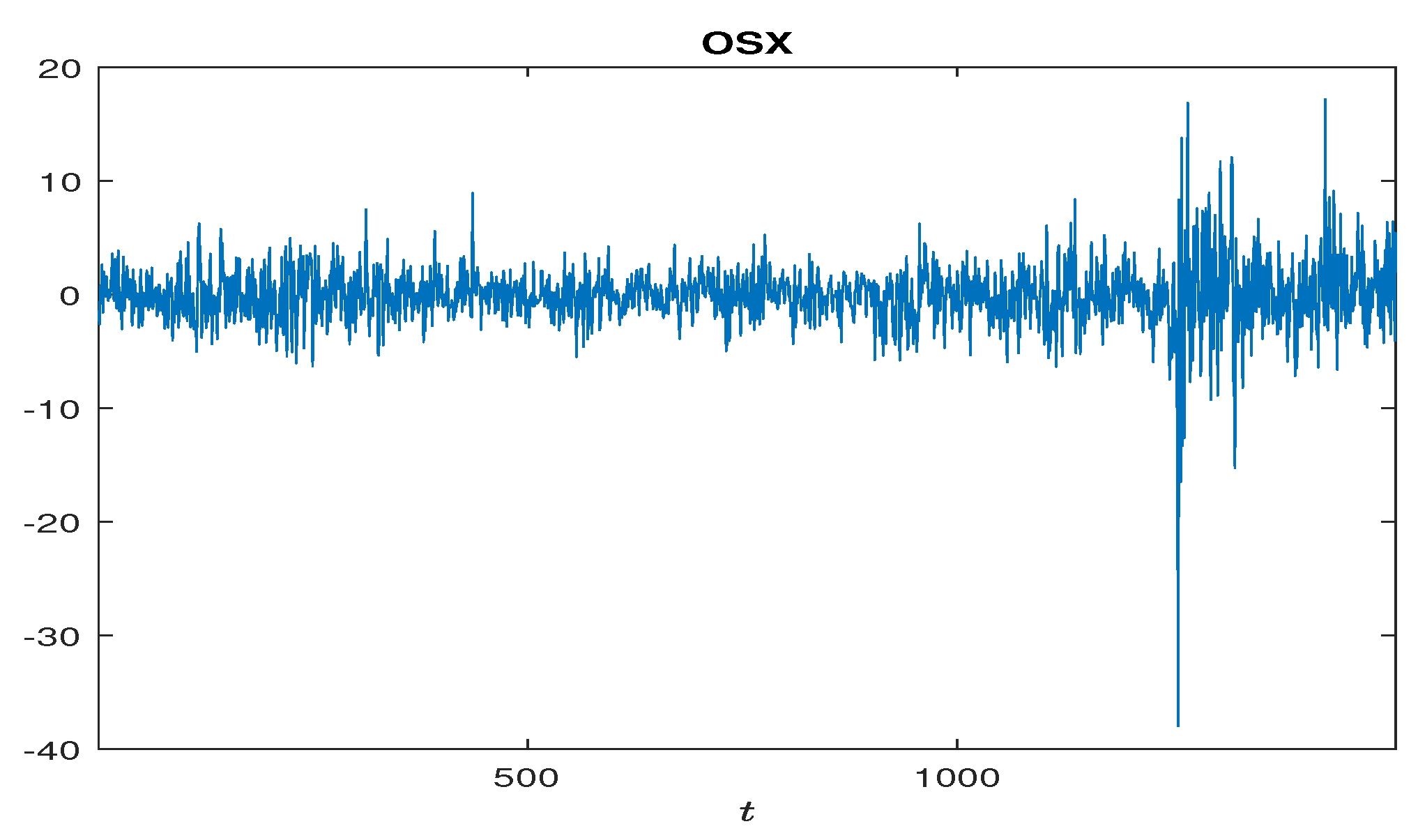
Next, this section considers the log returns ($\times 100$) of PHLX Oil Service Index OSX from 11 March 2015 to 10 March 2021, with a total of 1510 observations (see Figure 3). As before, we denote this log return series by ${\left\{y_t\right\}}_{t=1}^{1510}$, and obtain its estimate ${\widehat{\alpha }}_y=2.7960$ with $AD=0.7078$. This implies that $|y_t|$ has a finite second moment, but does not have a finite fourth moment. Hence, we apply the local QMLE method to get the following fitted model for $y_t$:

$$\begin{array}{cc}\hfill \left(\mathrm{OSX}\right)& \left\{\begin{array}{c}{y}_t=-0.0377+0.0239y_{t-1}+{\epsilon }_t,\hfill \\ \left(0.0589\right)\left(0.0307\right)\hfill \\ h_t=0.1329+0.1076{\epsilon }_{t-1}^2+0.8792h_{t-1}.\hfill \\ \left(0.0713\right)\left(0.0285\right)\left(0.0304\right)\hfill \end{array}\right.\hfill \end{array}$$

Unlike the fitted results for the four U.S. stock indexes above, the fitted AR coefficient for the OSX index is not significantly different from zero at the level of 5%, indicating that the oil market is efficient during the examined period.

6. Concluding Remarks

This paper studied the SWLSE of the ARMA model with GARCH noises and the residual-based QMLE for the GARCH model. The consistency and asymptotic normality of SWLSE were established under a little moment condition. The importance of the proposed estimators was illustrated by simulated data and four major stock indexes and one major oil index in U.S. The ARMA-GARCH model is very important in the risk management, see He et al. (2019). In practice, ones need to build the ARMA-GARCH model from the historical data. The major contribution of our paper is to present a way to build an efficient and reliable model for this purpose. Several potential future research topics are listed as follows: first, we may extend our procedure for the hybrid methodology that combines both ARIMA and ANN models with GARCH errors as in Zhang (2003); second, we could use our procedure to analyze the energy data and build an ARMA-GARCH model for the green energy, renewable energy, and bio-energy data as discussing in An and Mikhaylov (2020); third, we may explore a linear programming or a genetic algorithm to find the QMLE of ARMA-GARCH model as presented in An et al. (2021).

References

- An, Jaehyung, Alexey Mikhaylov, and Sang-Uk Jung. 2021. A linear programming approach for robust network revenue management in the airline industry. Journal of Air Transport Management 91: 101979. [Google Scholar] [CrossRef]
- An, Jaehyung, and Alexey Mikhaylov. 2020. Russian energy projects in South Africa. Journal of Energy in Southern Africa 31: 58–64. [Google Scholar] [CrossRef]
- Amemiya, Takeshi. 1985. Advanced Econometrics. Cambridge: Harvard University Press. [Google Scholar]
- Basrak, Bojan, Richard A. Davis, and Thomas Mikosch. 2002. Regular variation of GARCH processes. Stochastic Processes and Their Applications 99: 95–115. [Google Scholar] [CrossRef] [Green Version]
- Berkes, István, Lajos Horváth, and Piotr Kokoszka. 2003. GARCH processes: Structure and estimation. Bernoulli 9: 201–7. [Google Scholar] [CrossRef]
- Bollerslev, Tim. 1986. Generalized autoregressive conditional heteroskedasticity. Journal of Econometrics 31: 307–27. [Google Scholar] [CrossRef] [Green Version]
- Davis, Richard A., and Thomas Mikosch. 1998. The sample autocorrelations of heavy-tailed processs with applications to ARCH. Annals of Statistics 26: 2049–80. [Google Scholar] [CrossRef]
- Drost, Feike C., and Chris A. J. Klaassen. 1997. Efficient estimation in semiparametric GARCH models. Journal of Econometrics 81: 193–221. [Google Scholar] [CrossRef] [Green Version]
- Drost, Feike C., Chris A. J. Klaassen, and Bas J. M. Werker. 1997. Adaptive estimation in time series models. Annals of Statistics 25: 786–817. [Google Scholar] [CrossRef]
- Engle, Robert F. 1982. Autoregressive conditional heteroskedasticity with estimates of variance of U.K. inflation. Econometrica 50: 987–1008. [Google Scholar] [CrossRef]
- Francq, Christian, and Jean-Michel Zakoïan. 2004. Maximum likelihood estimation of pure GARCH and ARMA-GARCH processes. Bernoulli 10: 605–637. [Google Scholar] [CrossRef]
- Hall, Peter, and Qiwei Yao. 2003. Inference in ARCH and GARCH models. Eonometrica 71: 285–317. [Google Scholar] [CrossRef] [Green Version]
- He, Changli, and Timo Teräsvirta. 1999. Properties of moments of a family of GARCH processes. Journal of Econometrics 92: 173–92. [Google Scholar] [CrossRef]
- He, Yi, Yanxi Hou, Liang Peng, and Jiliang Sheng. 2019. Statistical inference for a relative risk measure. Journal of Business & Economic Statistics 37: 301–11. [Google Scholar]
- Hill, Jonathan B. 2010. On tail index estimation for dependent, heterogeneous data. Econometric Theory 26: 1398–436. [Google Scholar] [CrossRef] [Green Version]
- Johansen, Søren. 1995. Likelihood-based Inference in Cointegrated Vector Autoregressive Models. Oxford: OUP Oxford. [Google Scholar]
- Lange, Theis. 2011. Tail behavior and OLS estimation in AR-GARCH models. Statistica Sinica 21: 1191–200. [Google Scholar] [CrossRef] [Green Version]
- Ling, Shiqing. 1999. On the stationarity and the existence of moments of conditional heteroskedastic ARMA models. Statistica Sinica 9: 1119–30. [Google Scholar]
- Ling, Shiqing. 2003. Adaptive estimators and tests of stationary and non-stationary short and long memory ARIMA-GARCH models. Journal of the American Statistical Association 98: 955–67. [Google Scholar] [CrossRef]
- Ling, Shiqing. 2005. Self-weighted LAD estimation for infinite variance autoregressive models. Journal of the Royal Statistical Society: Series B 67: 381–93. [Google Scholar] [CrossRef]
- Ling, Shiqing. 2007. Self-weighted and local quasi-maximum likelihood estimator for ARMA-GARCH/IGARCH models. Journal of Econometrics 140: 849–73. [Google Scholar] [CrossRef]
- Ling, Shiqing, and Michael McAleer. 2002. Necessary and sufficient moment conditions for the GARCH(r, s) and asymmetric power GARCH(r, s) models. Econometric Theory 18: 722–29. [Google Scholar] [CrossRef] [Green Version]
- Ling, Shiqing, and Wai Keung Li. 1997. Fractional autoregressive integrated moving-average time series with conditional heteroskedasticity. Journal of the American Statistical Association 92: 1184–94. [Google Scholar] [CrossRef]
- Ling, Shiqing, and Michael McAleer. 2003a. Asymptotic theory for a new vector ARMA-GARCH model. Econometric Theory 19: 280–310. [Google Scholar] [CrossRef] [Green Version]
- Ling, Shiqing, and Michael McAleer. 2003b. On adaptive estimation in nonstationary ARMA models with GARCH errors. Annals of Statistics 31: 642–74. [Google Scholar] [CrossRef]
- Pantula, Sastry G. 1989. Estimation of autoregressive models with ARCH errors. Sankhyā: The Indian Journal of Statistics, Series B 50: 119–38. [Google Scholar]
- Setiawan, Budi, Marwa Ben Abdallah, Maria Fekete-Farkas, Robert Jeyakumar Nathan, and Zoltan Zeman. 2021. GARCH (1, 1) models and analysis of stock market turmoil during COVID-19 outbreak in an emerging and developed economy. Journal of Risk and Financial Management 14: 576. [Google Scholar] [CrossRef]
- Weiss, Andrew A. 1986. Asymptotic theory for ARCH models: Estimation and testing. Econometrics Theory 2: 107–31. [Google Scholar] [CrossRef] [Green Version]
- Zhang, G. Peter. 2003. Time series forecasting using a hybrid ARIMA and neural network model. Neurocomputing 50: 159–75. [Google Scholar] [CrossRef]
- Zhang, Rongmao, and Shiqing Ling. 2015. Asymptotic inference for AR models with heavy-tailed G-GARCH noises. Econometric Theory 31: 880–90. [Google Scholar] [CrossRef]
- Zhang, Wenjun, and Jin E. Zhang. 2020. GARCH option pricing models and the variance risk premium. Journal of Risk and Financial Management 13: 51. [Google Scholar] [CrossRef] [Green Version]
- Zhu, Ke, and Shiqing Ling. 2011. Global self-weighted and local quasi-maximum exponential likelihood estimators for ARMA-GARCH/ IGARCH models. Annals of Statistics 39: 2131–63. [Google Scholar] [CrossRef]
- Zhu, Ke, and Shiqing Ling. 2015. LADE-based inference for ARMA models with unspecified and heavy-tailed heteroscedastic noises. Journal of the American Statistical Association 110: 784–94. [Google Scholar] [CrossRef] [Green Version]
Figure 1.
Parameter regime of with .
Figure 2.
Log returns () of DJIA, NASDAQ, NASDAQ 100, and S&P 500 from 11 March 2015 to 10 March 2021.
Figure 3.
Log returns () of OSX from 11 March 2015 to 10 March 2021.