
Children and Life-Cycle Consumption

Department of Economics and Finance, Brunel University, London UB8 3PN, UK
J. Risk Financial Manag. 2022, 15(2), 42; https://doi.org/10.3390/jrfm15020042
Submission received: 12 November 2021
/
Revised: 31 December 2021
/
Accepted: 5 January 2022
/
Published: 19 January 2022
(This article belongs to the Special Issue Applied Financial Econometrics)
Abstract
:This paper investigates the role of children in explaining the life-cycle pattern of consumption (which is hump-shaped since it is higher in the middle of life and lower at the beginning and end of life). Unlike previous studies, a true panel of U.K. households was exploited to investigate whether currently childless households that anticipate having children behave differently from similar households that do not anticipate children. Spending for each group at different ages was estimated using a simple kernel regression. The paper finds that those households that anticipate children, when compared to households that do not anticipate children, do not seem to significantly reduce total spending before having children, nor do they significantly increase total spending after children arrive. Hence, children do not seem to fully explain the hump shape of consumption over the life-cycle.
1. Introduction
This paper explores the role of children in explaining the pattern of consumption over the life-cycle. In particular, it investigates whether households inter-temporally substitute consumption from periods without children towards periods with children. Ever since Thurow (1969), and more recently Browning et al. (1985) and Carroll and Summers (1991), among others, researchers have noticed how consumption and income appear to follow each other closely over the life-cycle. Both consumption and income display an inverted U-shape (or hump), being higher in the middle and lower at the beginning and at the end of the life-cycle. This correlation contradicts the simplest version of the standard life-cycle model of consumption in which households smooth consumption between periods of high income and periods of low income, holding the expected marginal utility of consumption constant. The contradiction is because the simplest version of the life-cycle model predicts that consumption can only either monotonically increase or monotonically decrease over time.
One popular argument for the “hump” in the household’s life-cycle consumption is that the standard life-cycle consumption model ignores changes in household composition. Household size changes over the life-cycle when a couple starts a family and eventually the children grow-up and leave the household. Family size and composition are thus a compelling candidate explanation for the observed behaviour of consumption over the life-cycle. A number of influential papers, such as Irvine (1978) and, more recently, Attanasio et al. (1999) and Browning and Ejrnaes (2009) have strongly argued for the role of family composition in explaining the observed pattern of consumption over the life-cycle and its close relationship with household composition. Identification in these papers exploits the timing of children and of consumption in the life-cycle, showing that they are contemporaneous (e.g., household size is largest when household spending is largest). The importance of this research agenda is underlined by the survey of consumption behaviour by Browning and Crossley (2001), who stated “there is now an emerging consensus that this important empirical regularity can be explained by some combination of precautionary savings (prudence) and demographic changes over the life-cycle (children)”.
This paper also investigates the role of children in explaining the hump in consumption, using the 1992–2005 wave of the British Household Panel Survey (BHPS). The paper concentrates on the period before and immediately after children first arrive in the household, which, to the best of our knowledge, has not been the specific focus of previous studies: the paper concentrates on the first child since this is where one might expect the effect to be largest. Unlike previous studies, this paper investigates the effect of children by contrasting the behaviour of those households that anticipate children and those that do not: hence, the identification of the effect of children on consumption is not from the timing of children and of consumption, which could be problematic if they are also related to the timing of income, but rather from the fact that not all households anticipate having children.
The paper shows that there are differences between households in whether they expect to have children and that these expectations are informative since those who expect to have children are more likely to have children. The question becomes whether the spending and saving behaviour of households also differs. If children explain the hump in the consumption over the life-cycle1, then those households that anticipate children should spend less before children arrive and more after children arrive when compared to similar households that do not anticipate children. If anticipating children is unrelated to (changes in) income over the life-cycle, then it is merely necessary to compare the behaviour of households who do and who do not anticipate children. This approach exploits the fact that not all households anticipate that they will have children. The results, in most cases, will show that those who anticipate that they will have children are genuinely more likely to have children, and have similar levels of income, when they are compared with households that do not anticipate children. However, while in some cases, these households differ in their food and utilities consumption, in most regressions, they do not differ in their overall level of spending.
A more detailed motivation is provided in Section 2, together with some of the basic facts about consumption and income over the life-cycle. The data are introduced in Section 3. The analysis in Section 4 starts by looking at differences in income and consumption for households who eventually have children, before looking at whether the household anticipates children. In the paper, there are two different ways of dividing households between those who anticipate children and those who do not: Section 4.2 looks at how the directly reported expectations about having children affect behaviour; Section 4.3 looks at households who believe children are important; Section 4.4 compares same-sex couples with opposite-sex couples. In each case, the results of a kernel regression are displayed, together with some confidence bounds. There are some final remarks about the analysis in Section 5.
2. Literature Review
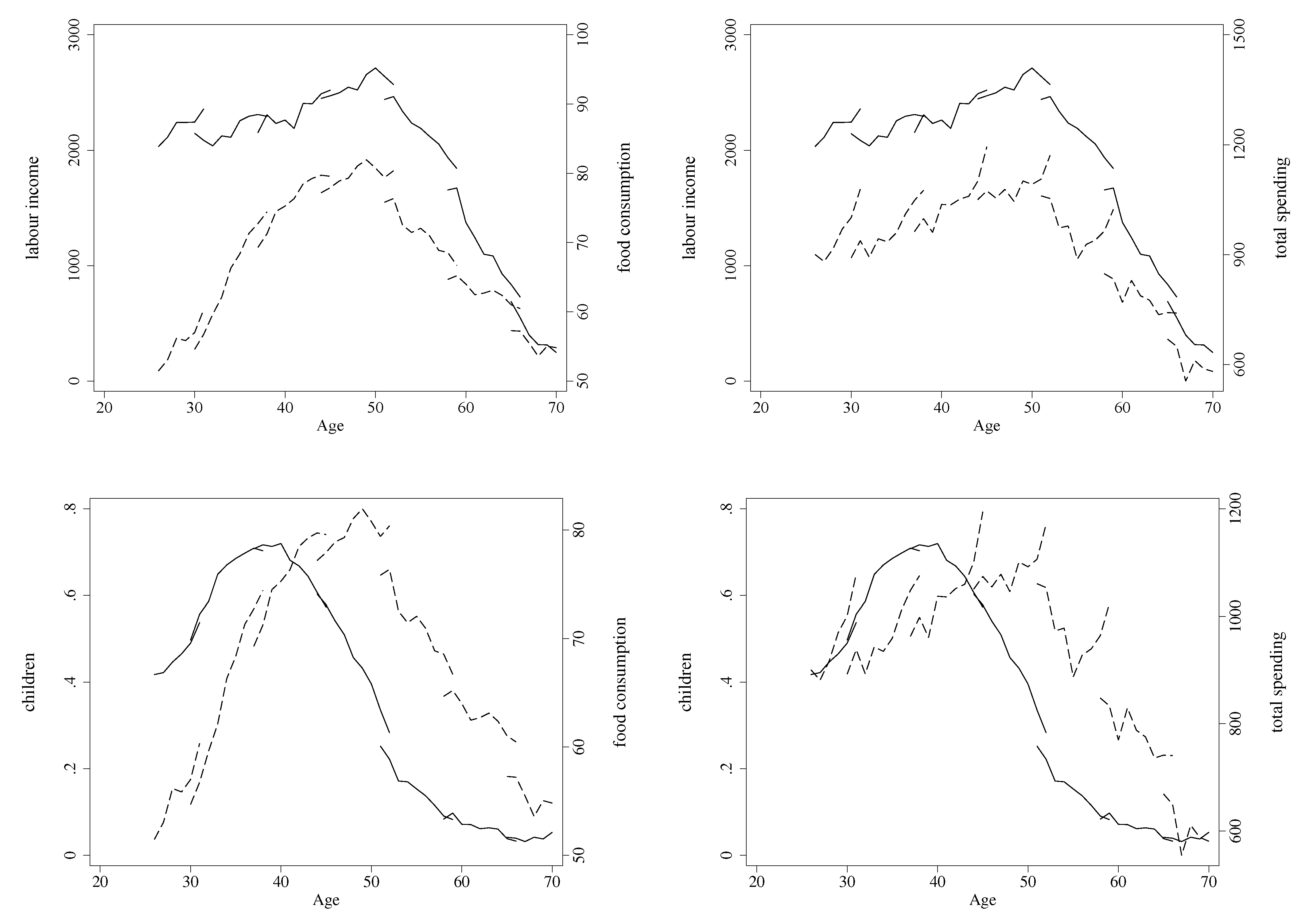
Using data from the BHPS (the data are described in detail below), the top half of Figure 1 shows how income and consumption seem to follow each other over the life-cycle, as first highlighted by Thurow (1969). These pictures were constructed using different year-of-birth cohorts and plotting the average level of income or consumption each month against the average age of the year-of-birth cohort in each year (where the first cohort is formed by household heads born between 1972 and 1978; the second between 1965 and 1971; the last between 1929 and 1936). On average, there are over 1000 observations in each cohort-year cell. There is a separate plot for each year, and succeeding years for the same cohort are joined by a dashed line for consumption, and a solid line for income. In each case, income and consumption are on different scales: the scale for income is on the left-hand side, while the scale for consumption is on the right-hand side. The top-left panel plots real monthly labour income and real monthly food consumption over the life-cycle, while the top-right panel shows real monthly labour income and real monthly total spending. In both cases, the figure shows that income and consumption seem to follow the same pattern over the life-cycle. Both income and consumption seem to increase slowly from young ages until they peak at around age 50, and then, they both fall steeply with both income and consumption lowest for the oldest households in the sample, at age 70. These results are similar to those previously reported by Carroll and Summers (1991) and Gourinchas and Parker (2002) for non-durable consumption and by Fernandez-Villaverde and Kreuger (2007) for durables (in the presence of durables, consumption and spending are not the same thing).
The closely matching pattern of income and of consumption, particularly when looking at total spending, is striking. A number of explanations for this phenomenon have been offered in the literature. For example, Skinner (1998), and Carroll (1997) both emphasised the role of precautionary motives for saving, while Deaton (1991) discussed whether credit constraints could explain the hump. More recently, Jorgensen (2017) also argued that a combination of credit constraints and precautionary savings are causing the hump. Having time-inconsistent preferences has also been offered as an explanation of the hump in consumption (this literature is extensively reviewed in Park 2012). More recently, Kraft et al. (2017) discussed whether “habits” can explain the hump. Several previous studies have also investigated the possible causes of the sharp drop in consumption after age 50. Banks et al. (1998) emphasised how consumption falls upon retirement, which has given rise to a substantial literature on the “retirement-savings puzzle”. An important explanation for the sharp post-retirement drop in spending, given in Aguiar and Hurst (2005), is that households substitute home production for spending (e.g., eating at the home rather than outside). Aguiar and Hurst (2007) extended this argument by showing that there are considerable differences in the time spent shopping at different ages, which explains the hump as due to the substitution between shopping time and the level of spending.
This paper, rather than comparing households at different ages, compares different household types at each age in the sample. It concentrates on the early part of the life-cycle: the period before and immediately after children arrive in the household. Recall that one popular candidate explanation for the hump in consumption is that households have children in the middle of the life-cycle, and hence increase spending for reasons exogenous to income. That children can explain the correlation over the life-cycle between income and consumption was first explored by Irvine (1978) and, more recently, by Blundell et al. (1994), by Attanasio et al. (1999), and by Gourinchas and Parker (2002). The later papers argued that account must be made of household size and composition when assessing the life-cycle model of consumption. They argued that demographics and non-certainty equivalence in the utility function can generate the hump-shaped profile to consumption over the life-cycle without requiring credit constraints or myopia. Fernandez-Villaverde and Kreuger (2007) and, more recently Fernandez-Villaverde and Kreuger (2011) used adult equivalent scales to adjust household consumption by family size. They argued that household size can explain 50% of the hump in household consumption, but in contrast to the other papers, believed that children cannot fully explain the hump.
The bottom half of Figure 1 plots the pattern of children over the life-cycle against food consumption and against total spending. It shows that children also display a hump-shaped pattern over the life-cycle, peaking in the middle of the life-cycle and being lower at the beginning and end of the life-cycle. However, compared to consumption, it seems that the pattern for children peaks earlier in the life-cycle. Its highest point is at around 40, while consumption is highest at around 50. Browning and Ejrnaes (2009) argued that if older children cause higher consumption than younger children, then household composition can nevertheless fully explain the hump-shaped pattern to consumption. Hence, the later peak for consumption need not reject that children are causing the life-cycle pattern to consumption.
A key problem in this approach is that the role of household composition has not been investigated using a true panel (where the same household is followed over a number of years). Due to data limitations, previous studies, such as Attanasio et al. (1999), or Fernandez-Villaverde and Kreuger (2007), were only able to construct a synthetic panel from a time series of cross-sections whereby membership of the panel is based on observable factors that do not change over time. Using synthetic panels, however, means that one can only investigate the timing of life events. Thus, the existing literature has shown that, on average, the incidence of children is highest at the same time as the level of consumption peaks (and this remains true even if the data are further partitioned on additional observable characteristics such as education). That is, there is an identification problem in separating the effect of children from any other possible effects of age or other age-related taste-shifters that change the level of consumption independently of children.
This paper addresses the identification problem by using a true panel and by exploiting the fact that not all households have children. If not all households plan to have children, but all households are observed over time, then the identification problem is solved since we have a natural experiment: those households that anticipate children can be directly compared with those who do not. A valid test of the argument that children drive (a large part of) consumption over the life-cycle is to investigate whether there are systematic differences over time between the consumption behaviour between these two groups. If children explain the hump-shaped pattern of life-cycle consumption, then childless couples ought, ceteris paribus, to consume less in the middle of their lives, and correspondingly more both at the beginning and at the end of their lives. We show that households that eventually have children raise spending in early middle age compared to childless households. However, we also show that households who have children do not have the same income levels as households who do not. This causes an identification problem in the Euler equation approach as children predict permanent income; hence, adding children to the Euler equation will not distinguish between changes in tastes and changes in permanent income.
The relationship between consumption and children is more subtle if childlessness is often unplanned, perhaps because one or other partner is unexpectedly infertile. Households who plan to have children may defer their spending when they are young, only to later discover that they are unable to have children.2 Such households may well mimic the behaviour of households with children (at least at younger ages) even though these children do not subsequently arrive. This means that the key issue is whether the household intends to have children at younger ages. To properly investigate the role of children, Browning and Crossley (2001) argued for the need for a long panel of households that report their fertility plans. This paper exploits previously unexplored information on fertility plans in the BHPS, a panel of British households that records information on income and spending.
3. Data and Methods
The British Household Panel Survey (BHPS) is a survey of 10,000 individuals from England, Scotland, and Wales who were first interviewed in 1991 (more details on the survey are provided by Taylor and Brice 1999). This study used data for the years 1992 to 2005. In the BHPS, each household member is asked a variety of questions about his/her income, attitudes, and consumption, as well as other details of the household, such as family composition. Households are re-interviewed each year so that their behaviour can be followed over time and thus form a panel.
The questions about attitudes means that households discuss their plans for children at regular intervals. The panel nature of the data means that the subsequent behaviour of these households can be explored, and several important questions answered. For example, are children more likely to arrive in households that respond positively to questions about having children? Are the income profiles of households that anticipate children different from households that do not anticipate children? Are their consumption profiles different? For the analysis to be meaningful, it is crucial that how households respond to the questions about their plans for children is correlated with whether they subsequently have children. Moreover, if their incomes are systematically different, it will not be a surprise if their consumption behaviour is also different (and will certainly not reject the life-cycle model augmented by children). Hence, the paper not only compares the consumption behaviour of the different households, but also their incomes and whether they have children.
In the BHPS, income is reported in considerable detail, with households reporting their income during each calender month and with separate questions on labour income, overtime, each of the individual items of social security payments, and on such things as dividends, rent, and other individual items of unearned income. This study investigates the role of monthly income from employment in the labour market. All values are deflated so that they were reported in 2003 prices (using the reported CPI price index).
The survey also includes separate questions on several categories of consumption. Households are asked to report their total weekly food and grocery spending and their monthly spending on utilities (with separate questions on individual items) and on household durables over the last year. The level of detail of the questions on utilities and durables is high (there are separate questions on each individual item such as dishwashers, satellite equipment, and CD players, as well as the separate items making up spending on utilities). However, while the spending on utilities and on durables is the actual amount, the response to the spending on groceries is chosen from one of twelve bands. These responses have been turned into actual spending by assigning a value corresponding to the middle value of the band (so that, for example, a household reporting spending in the band GBP 120–140 per week is assumed to spend GBP 130). From Wave 6 of the survey, individuals, rather than households, were also asked about their monthly spending on eating out and on leisure activities. These responses are also given by choosing from 12 bands, with the same procedure followed as for groceries (and household spending is the sum of each household member’s spending). Lastly, households were also asked about their spending on housing.3
The analysis in this paper considers, first, real monthly spending on food and utilities and, second, real total monthly spending. The second category is constructed as the sum of each of the individual categories of spending that are reported in the survey. However, as spending on leisure and on eating out were not included in the earlier waves of the survey, this means that household spending is not completely comparable for the the first six waves and for the waves that follow. However, because the primary focus is on comparing and contrasting the behaviour of different groups of households at each point in time, this is not a serious problem. This study considers whether, for instance, households that expect children behave differently compared to households that do not expect children; hence, what is crucial is that the consumption behaviour of these two groups at a point in their life-cycle can be compared, rather than how the behaviour of either group behaves over time.
Using the BHPS for this analysis has a number of advantages. First, the length of the panel (which is 15 years) means that the same household can be followed over time, meaning we have a natural experiment. Hence, households with different expectations about the future can be compared over time. This would not be possible using synthetic panels constructed from the data in, for instance, the Family Expenditure Survey in the U.K. or the Consumer Expenditure Survey in the U.S. Second, while the data on consumption are not measured completely accurately, this does allow the construction of a much broader measure of spending than could be constructed using the U.S. survey, the Panel Study of Income Dynamics. Third, income is measured accurately, which means that income can be compared for each of the types of households that are investigated. Fourth, a major part of the analysis in this paper is to exploit attitudinal questions that are contained in the survey. These types of questions are rather rare in households surveys, especially in surveys that are panels, and contain the requisite information on income and on consumption. Of course, despite these crucially important advantages, the fact that consumption is not measured accurately (since some components of consumption, but not all, are bracketed) is an important limitation. However, as will be seen, the detail in the survey is sufficient that groups can sensibly be compared.
Throughout the rest of the paper, income, children, and consumption are plotted against age for those who reasonably anticipate having children and those who do not. In each case, the level of income (or children or consumption) was calculated by using a kernel regression with a variety of explanatory variables included in the regression (such as race, cohort, and education; omitting the controls and choosing a fixed bandwidth give broadly the same results). All the regressions used a Gaussian kernel function, with the bandwidth being chosen through cross-validation. The main results are reported in the next section; additional supporting evidence is reported in the Appendix A.
4. Results
4.1. Whether the Household Eventually Has Children
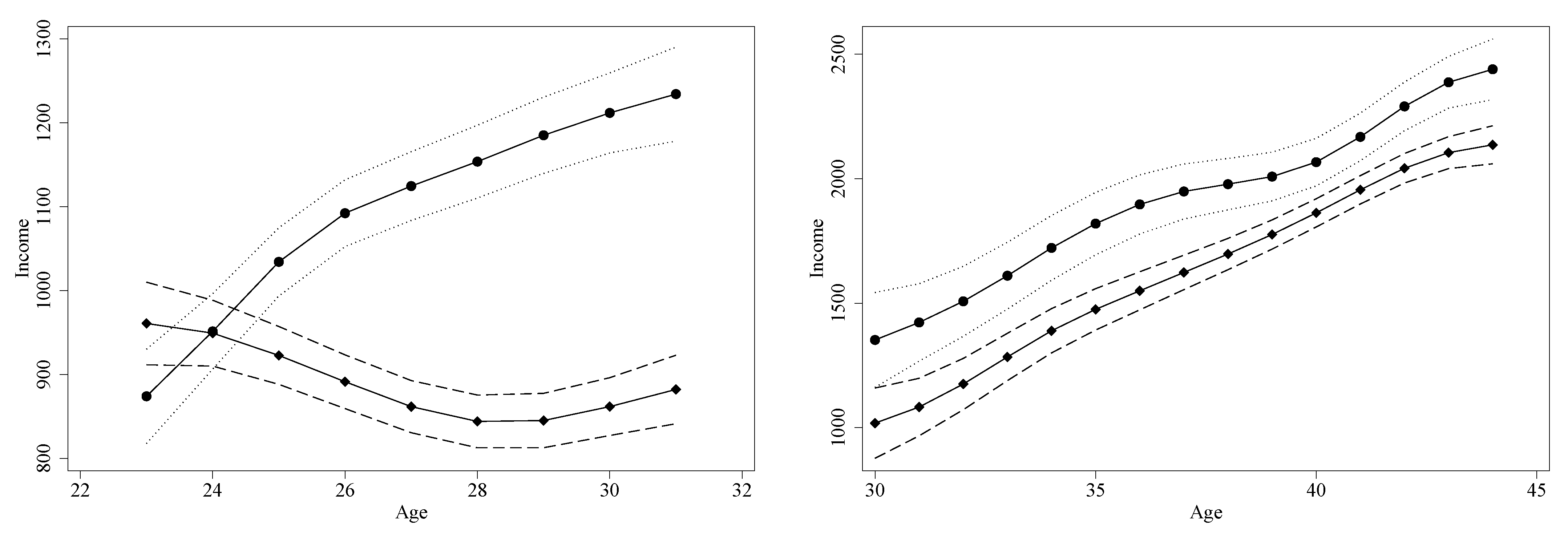
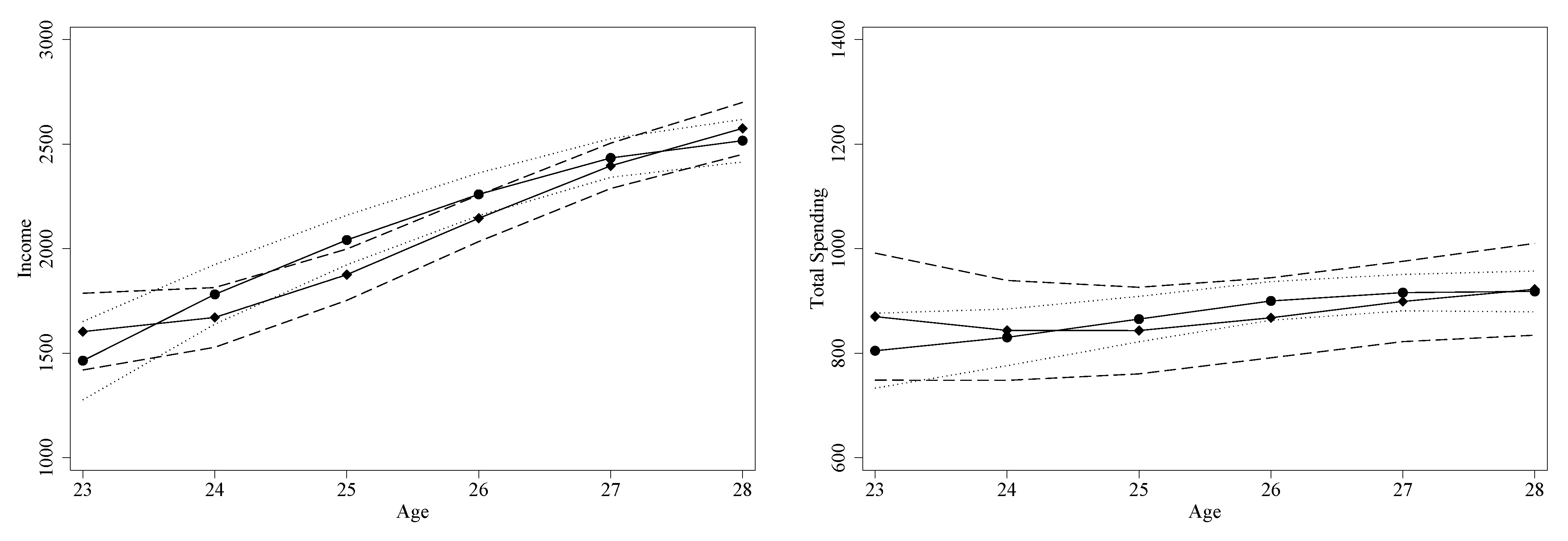
The analysis starts by looking at two different year-of-birth cohorts and whether the household eventually (e.g., by the end of the period of analysis) has children. The two cohorts are those born between 1964 and 1970 and those born between 1971 and 1977. Since the age of the later-born cohort is quite low at the beginning of the sample period, the figures only report results for this cohort from Wave 7. Figure 2 plots each cohorts’ labour income against their median age, with separate plots for those households that eventually have children and those households that do not. The figure shows that households that have children, except for the youngest waves, consistently have higher levels of income than those households that do not eventually have children. This difference in maintained through each wave of the data that we plot.
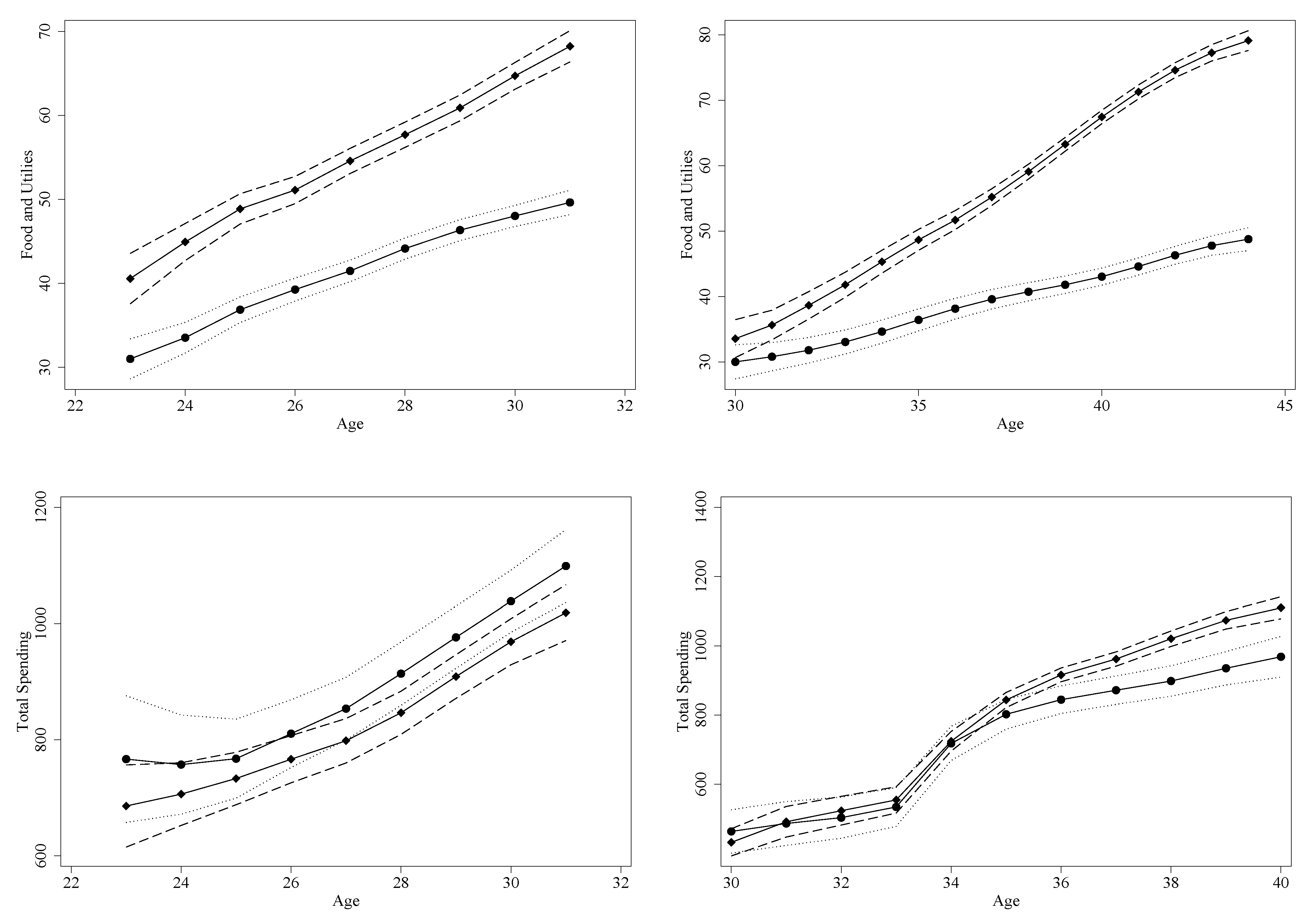
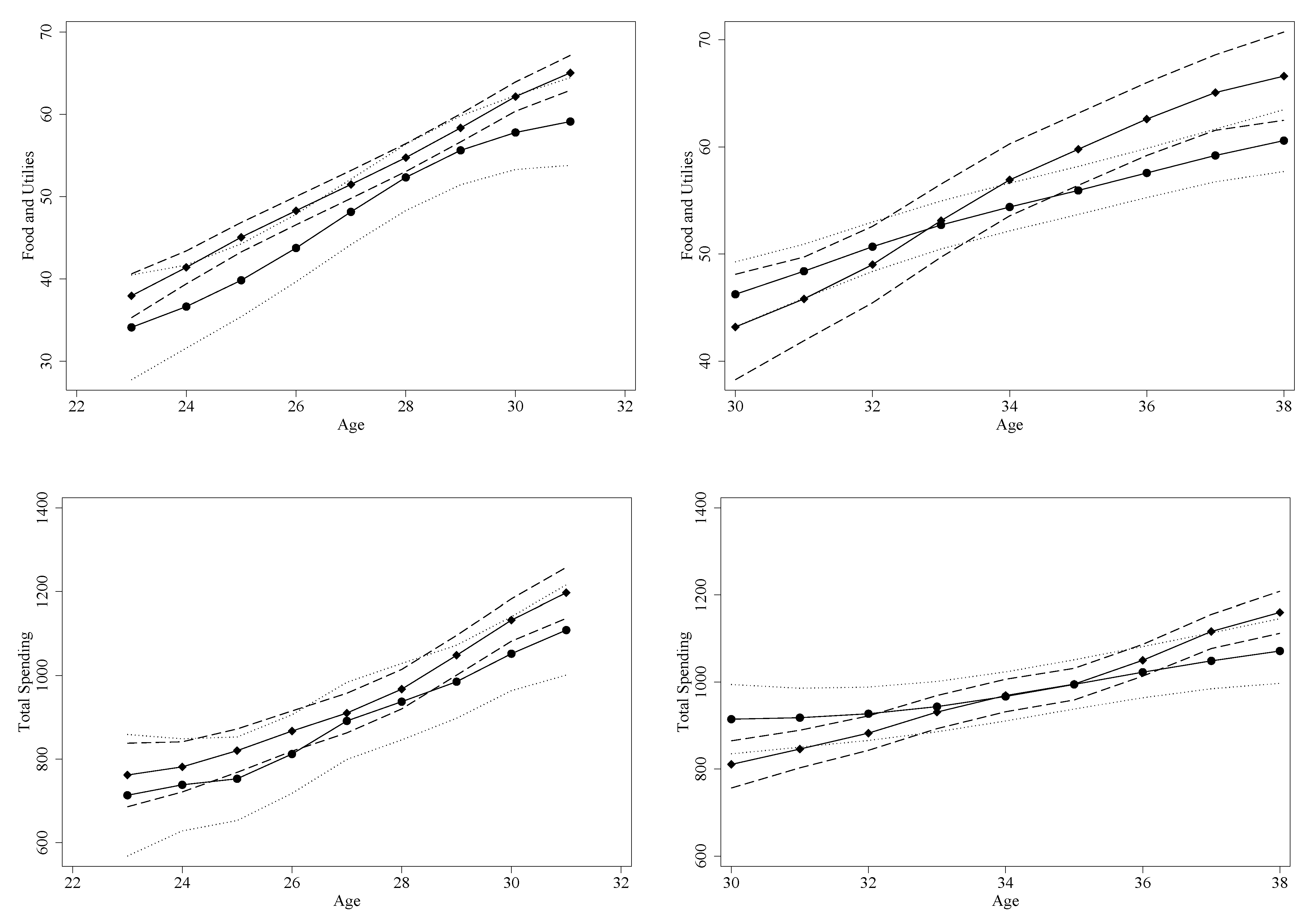
Figure 3 plots the level of consumption for each cohort (again divided between those households who eventually have children and those who do not). The results showed that food and utilities consumption differ between the two groups for both the younger and the older cohort. However, when looking at total spending (which includes durable goods), for the younger cohort, there is no difference between the spending made by those who will ultimately have children and those who will not. The older cohort, on the right-hand side of the figure, also shows that there is no difference in spending at younger ages and that spending only diverges when households are over 35 (this is, when the confidence intervals no longer overlap).
These results showed that income significantly differs between those who have children and those who do not. The results also show that, eventually, total spending in households that have children also diverges from households who do not: that is, households that eventually have children have a higher income in the long-run (e.g., higher permanent income) than households that do not. We would expect this higher life-cycle income to result in higher consumption, and indeed, this is what we observe in Figure 3. Hence, we are not able to deduce whether the extra consumption in households with children is a result of having children or the higher permanent income. This result is also problematic for the Euler equation approach, since it is difficult to disentangle the fact that children might increase consumption from the fact that having children is cross-sectionally correlated with permanent income. To address this problem, the paper tries to draw inference from attitudes toward children. We have in mind that poorer households may wish to have children, but never have children. The paper shows that when concentrating on these attitudes, the differences in income between those with positive attitudes toward children and those with negative attitudes is much smaller, and hence, differences in their consumption behaviour truly test for the effect of children without being contaminated by income effects.
4.2. Whether the Household Expects to Have Children
4.2.1. The 1992 Wave
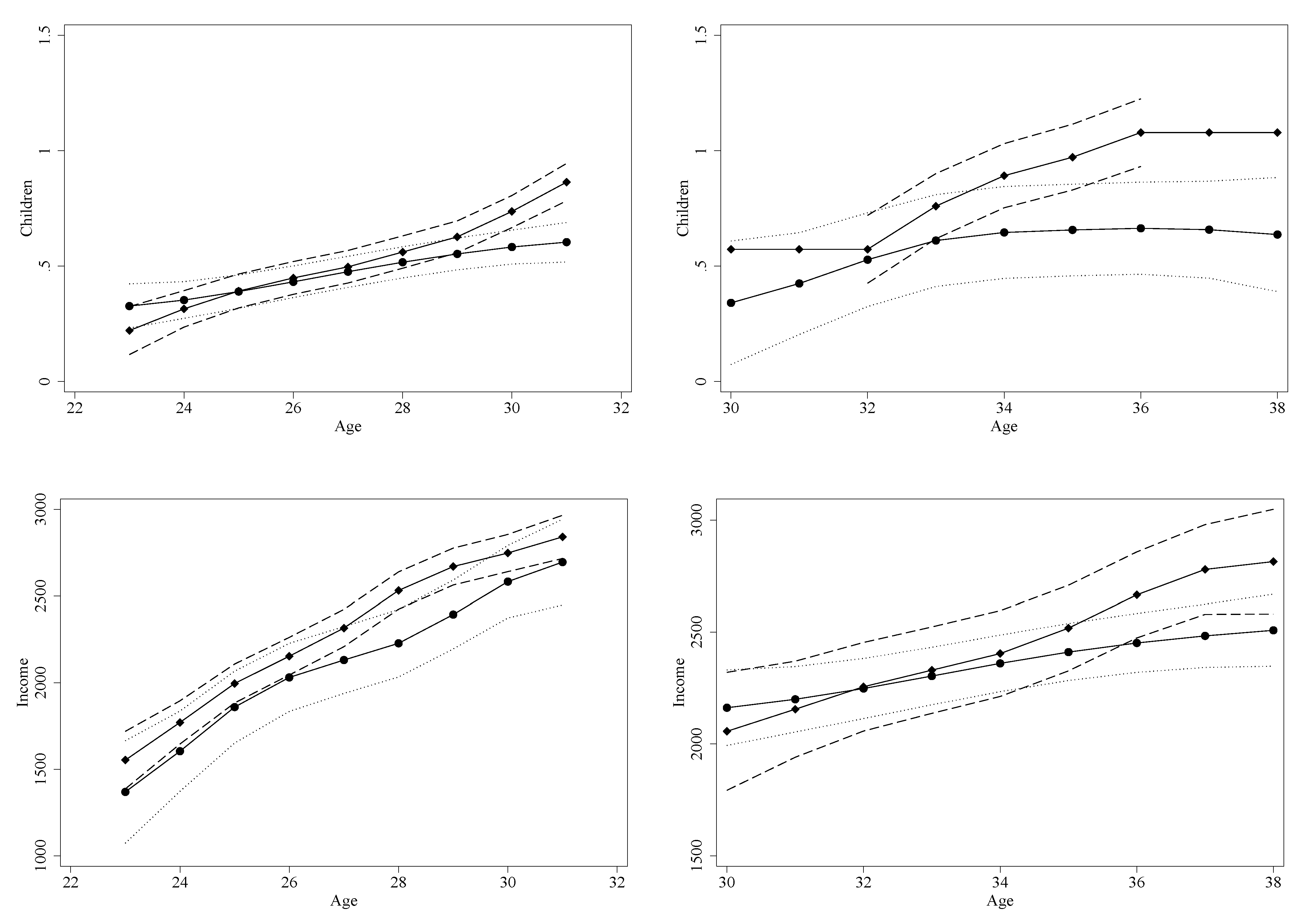
In the 1992 wave of the BHPS, household members of childbearing age were asked whether it was likely that they would have any (more) children. From this, two groups were constructed: those households that reported that they expect to have children and those who reported that they do not. The behaviour of two year-of-birth cohorts was investigated: those born between 1964 and 1970 and those born between 1971 and 1977. Since the age of the later-born cohort are quite low at the beginning of the sample period, the figures only report results for this cohort from Wave 7. Attention is also restricted to those households who are childless at the time the question was asked: this should make the test more dramatic since one would expect the first child to have a larger effect on behaviour than subsequent children. To make a fair comparison, attention was further restricted by also excluding households that do not have children in the following two years: hence, only those households who were childless in 1992 (the first year in which the household is surveyed), and remained childless through to 1994, were included in the sample. Attempting to include earlier-born cohorts resulted in too few households to form sensible cell sizes, since relatively fewer of these older households were childless at the time of the survey. Moreover, at older ages, relatively few households can reasonably expect to have children. (There are on average nearly 300 households in each year-cohort cell in the later-born cohort and over 350 households in the earlier-born cohort, which were childless in 1992; around 30% did not expect kids).
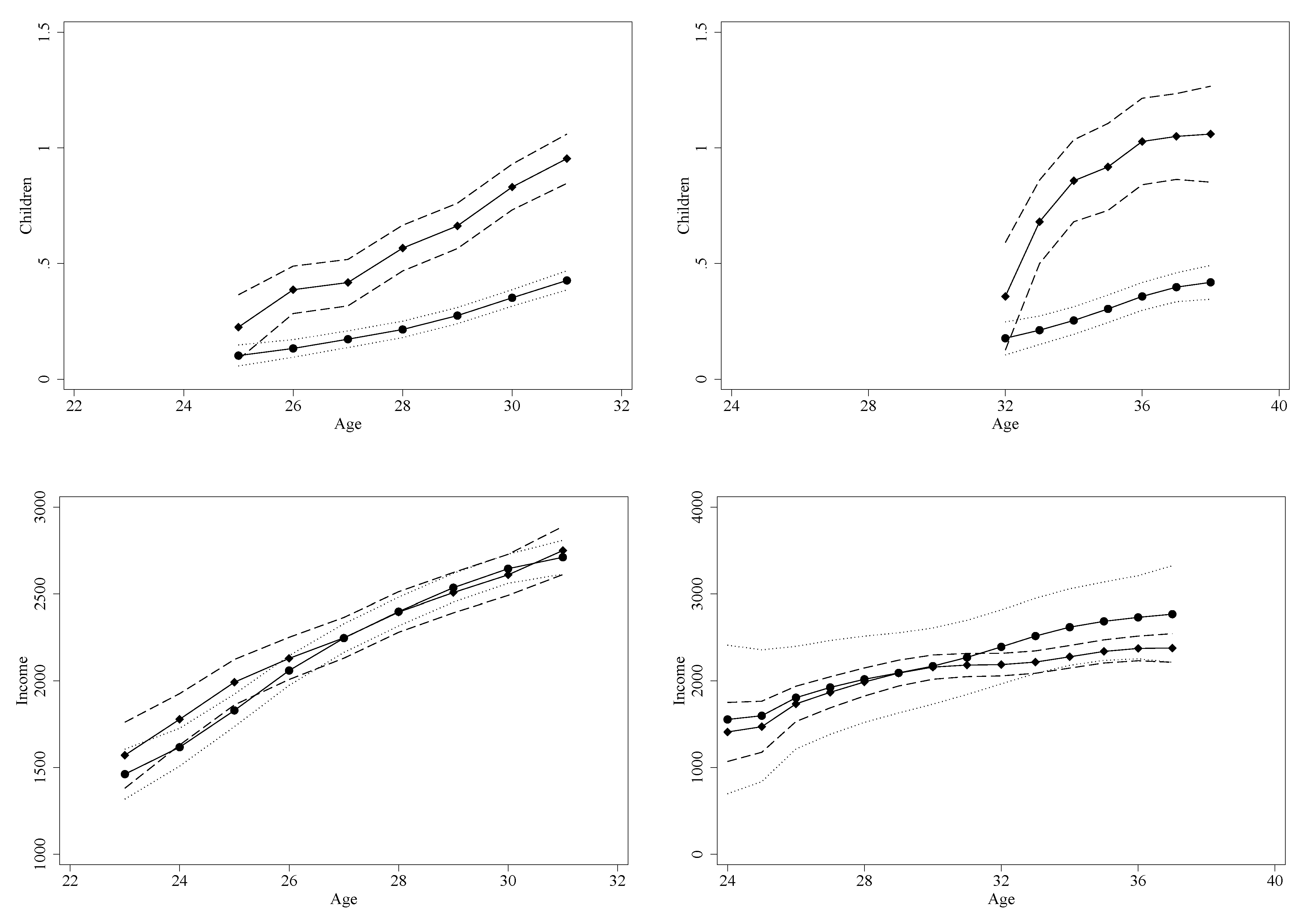
The top half of Figure 4 shows the two cohorts, with the median age of each cohort plotted on the horizontal axis and the estimated number of children in the household on the vertical axis. These estimates were constructed using kernel regressions and control for education, cohort, and race, and as throughout paper, the bandwidth was chosen through cross-validation. The figures are plotted for all years from 1998. The upper-left panel shows the later-born (or younger) cohort, while the upper-right panel shows the earlier-born (or older) cohort. Two solid lines are plotted, one for those households that expect to have children (plotted with diamonds) and one those households who do not expect to have children (plotted with circles). There are two dashed lines around the kernel estimates for the group who expects children, which shows the 95% confidence interval around the central estimates, and a dotted line marks the 95% confidence interval around the estimate for those who do not expect children in 1992 (a formal test of these differences are reported in Table 1 at the end of the paper).
For the younger cohort, the figure shows that there was no significant difference between the two groups (expecting children and not expecting children) in the average number of children that each group had up until end of the survey (testing at the 5% significance level). For both groups, the number of children increased, but it increased at a similar rate. The picture for the older cohort (in the top-right panel of Figure 4) was slightly different. When the average age of the cohort was below 34, there again seems to be no significant difference between the two household types, but the two lines diverge at older ages. It seems that at these older ages, those households who reported in 1992 that they expected to have children were significantly more likely to subsequently have children than households who reported that they did not expect to have children. This shows that the question can distinguish between the two groups in terms of subsequent behaviour. The bottom half of Figure 4 shows the kernel estimates for labour income for the younger and the older cohort. For the younger cohort, there was no significant difference in labour income, except at age 28. For the older cohort, labour income was significantly different only at age 37. Otherwise, the income levels of the two groups were broadly similar.
Overall, we can see that both groups at first had the same number of children, but for the older cohort, eventually, there was a significant difference in the number of children that households that expected to have children subsequently had. Thus, by comparing the consumption behaviour of the two groups, we can assess whether children are contributing to the hump-shaped profile of consumption over the life-cycle. If children are important in explaining the life-cycle pattern of consumption, we should see a significant difference in behaviour between these two groups: a household that expects to have children should reduce its consumption in the period before it has children and increase its consumption in the period after having children. That is, the household, according to theory, should inter-temporally substitute some of its consumption from the period before it has children to the period post-children.
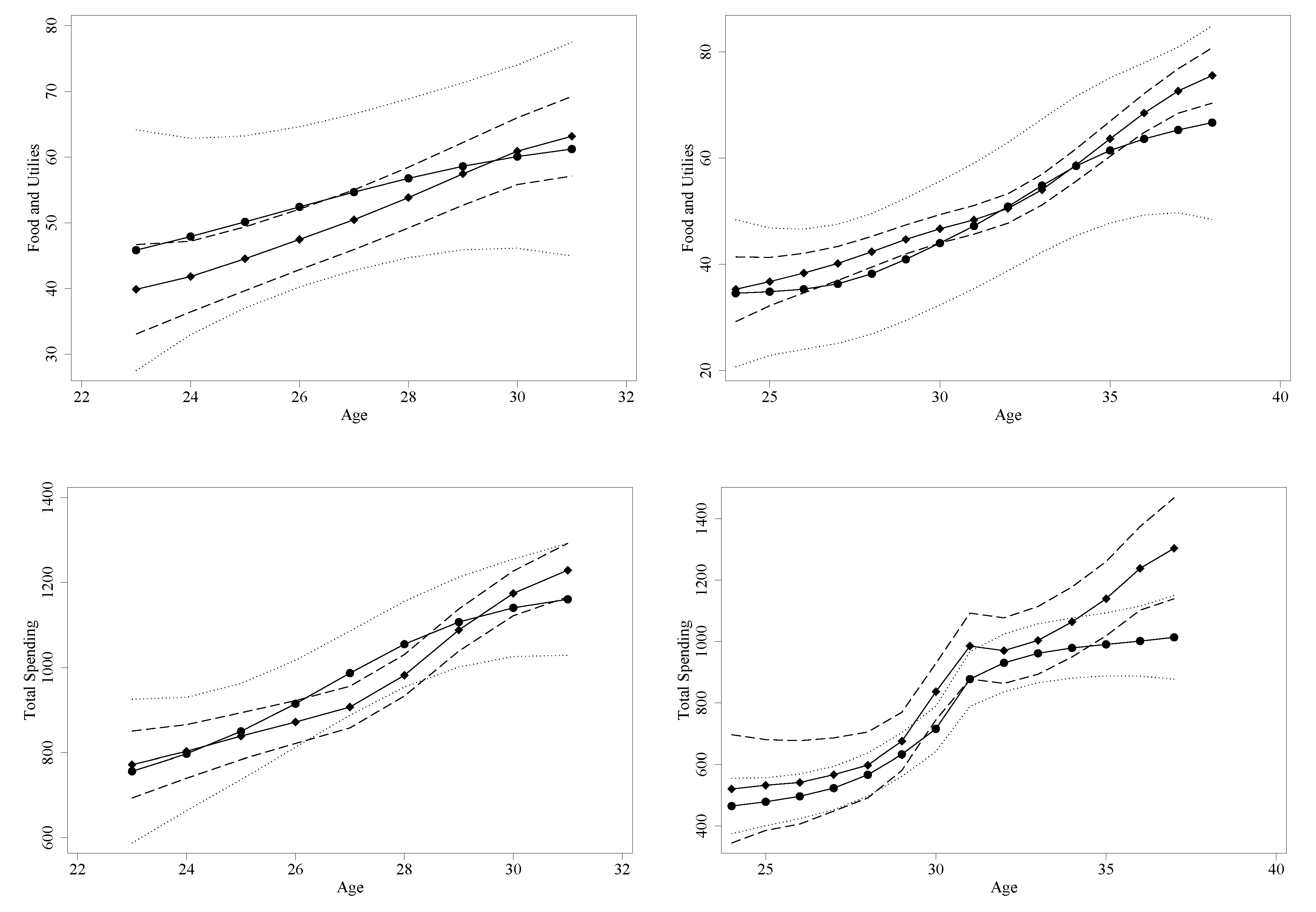
The top half of Figure 5 looks at food and utilities consumption for both household types. For the younger cohort, those who expected to have children (plotted with diamonds) had higher consumption (at the 5% significance level) in around half of the years included in the study. For the older cohort, there was no significant difference in food and utilities consumption in earlier years, but there were significant differences by the end of the sample period, with those who expected children consuming significantly more than those who did not expect children. Recall that if children cause households to move consumption from childless periods to periods when they have children, we should see households that expect to have children spending less in early periods and more in later periods. For the older cohort, we did indeed see households who expected to have children consuming more after the children arrived. The younger cohort, however, was consuming more in periods before children arrived when we would expect them to be reducing consumption. Overall, the results for food and utilities do not seem to offer clear supporting evidence for the thesis that children affect life-cycle consumption.
The bottom half of Figure 5 looks at total spending. It shows that there is no significant difference between the two groups for the younger cohort. It does not seem to matter that one group expects to have children and the other group does not: both groups showed the same spending behaviour over this part of the life-cycle. For the older cohort, the difference between the two groups was significant at age 31 and age 32 (which was when the two groups did not yet differ in the number of children in the household), but this was not significantly different at the end of the survey period. The results for the younger cohort were not what would be expected should children be causing households to inter-temporally substitute consumption. However, the results for the older cohort seem to support our central hypothesis, since those who expected children, but did not yet have children, had indeed reduced their spending.
4.2.2. The 1998 Wave
Households were also asked about whether they expected to have children in the 1998 wave of the data. Attention was again restricted to those households who did not have children either in the year in which they were asked the question, nor in the year following the survey. As before, the sample was divided into two groups: those who reported they expect to have children (plotted with diamonds) and those who reported they do not (plotted with circles). The top half of Figure 6 and Table 2 shows the the proportion of households that had children for each type of household in the years that followed the survey. The analysis was performed for the same two cohorts as before, again using kernel regressions, which control for race, education, and cohort. The figure shows that by the end of the sample period, for the older cohort, those households that reported that they expected to have children were significantly more likely to have children compared to households that reported that they did expect to have children. This finding is despite the fact that neither group had children when asked in the question in 1998. The results for the younger cohort, however, do not show a clear significant difference between the two groups.
The labour income profile of the two groups is shown in the bottom half of Figure 6. For the younger cohort, there was no significant difference in the income profiles of the two groups: those households that reported that they expected to have children in 1998 had the same income as those households that reported that they did not expect to have children. However, the story is somewhat different for the older cohort. Here, in the later years, the income of the two groups started to diverge, and the difference became statistically significant in the last three years (see Table 2).
Figure 7 plots the consumption profiles (tested in Table 2), of the two different groups, estimated using kernel regressions that control for race, education, and cohort (the top half shows food and utilities consumption, while the bottom half shows total spending). The jump in total spending for the older cohort at around age 30 was because from Wave 6, total spending included spending on leisure and on eating out (the younger cohort is not plotted for the years before Wave 6), which is not included in earlier years. (Recall that the test is to compare the spending of the two groups at each point in time; hence, the fact that extra items are included in spending in later periods does not affect the test.)
For the younger cohort, the consumption profiles were very similar, and there was no significant difference between the consumption profiles of those who expected children in 1998 and those who did not. For the older cohort, food and utilities consumption did not differ between those who expected children and those who did not, but total spending diverged for older ages. Those households who expected to have children in 1998, but did not yet have them, were spending more at the end of the sample period than those households that did not expect to have children. The top half of Figure 6 shows that these households were also more likely to have children at the end of the survey period. This might seem to be a confirmation of the theory. However, the bottom half of Figure 6 shows that the households that expected to have children in 1998 were earning more. A higher income itself will raise consumption, and this cause of the higher spending cannot be ruled out. Hence, these plots do not necessarily prove the case that children cause the life-cycle consumption profile observed in the data, but leave the question open.
Some further remarks are useful here, since it is surprising that among the 1998 childless households, those that expected children earned more in the years that followed compared to those that did not. In 1998, the average age of the older cohort was 31 (with households both older than this and younger than this within the cohort). At this age, many households already have children and will not be in either of the two groups since only childless couples were included. If more educated households are more likely to have children at later ages, then the sample of households that expect to have children is likely to have relatively fewer low-education households than might otherwise be expected, since such households disproportionately already have children. That better-educated women marry later and have children later was documented by McLanahan (2004). For the group that did not expect children, the less-well-educated households would not be selected out, and hence, this group may well contain relatively more of such households. This could explain the differences in the income profiles of the two groups for the older cohort.
4.3. Whether Having Children Is Important
In both the 1998 and 2003 waves, households were asked about the importance of having children. On a scale of one to ten, a score of 1 represented “not important at all” and a score of ten represented “very important”. Using this question, the sample of households was split into two groups: those households who said that having children is important (that report a score of eight or more) and those who said having children is not important (that report a score of seven or less). Moreover, attention was restricted to those households without children when the question was asked. If children can explain the hump-shaped pattern to consumption over the life-cycle, then we would expect there to be significant differences between the consumption behaviour of these two groups. First, we can expect those households who say having children is important to be more likely to have children. Second, if having children is important, then these households can be expected to save when young so that they can increase their level of consumption when they are older, and there are children in the household. It could also be possible that these households spend more on their children than those households who do not believe having children is important; this would further exaggerate the differences in the life-cycle spending profile between the two groups. This study investigated the response to the questions in both 1998 and 2003, each in turn.
4.3.1. The 1998 Wave
For the 1998 survey, attention was restricted to those households who did not have children in 1998, but nevertheless reported that having children is either “important” or “not important”. As before, the sample was divided into two groups based on the year of birth: those born between 1971 and 1977 and those born between 1964 and 1970. There were nearly 200 households in each year-cohort cell for the earlier-born cohort (around two-thirds believed having children is important) and 250 households in the later-born cohort (where nearly three-quarters strongly wanted children). Since the age of the earlier-born cohort was quite low, the figures only report results for this cohort from Wave 7. This paper did not investigate households born earlier than 1964 since the average age of the members of the next cohort when the question was asked was around 40. Among such households, relatively few households that did not have children believed that having children is important. Many of these households must also believe that they will not necessarily have children, even if they want them.
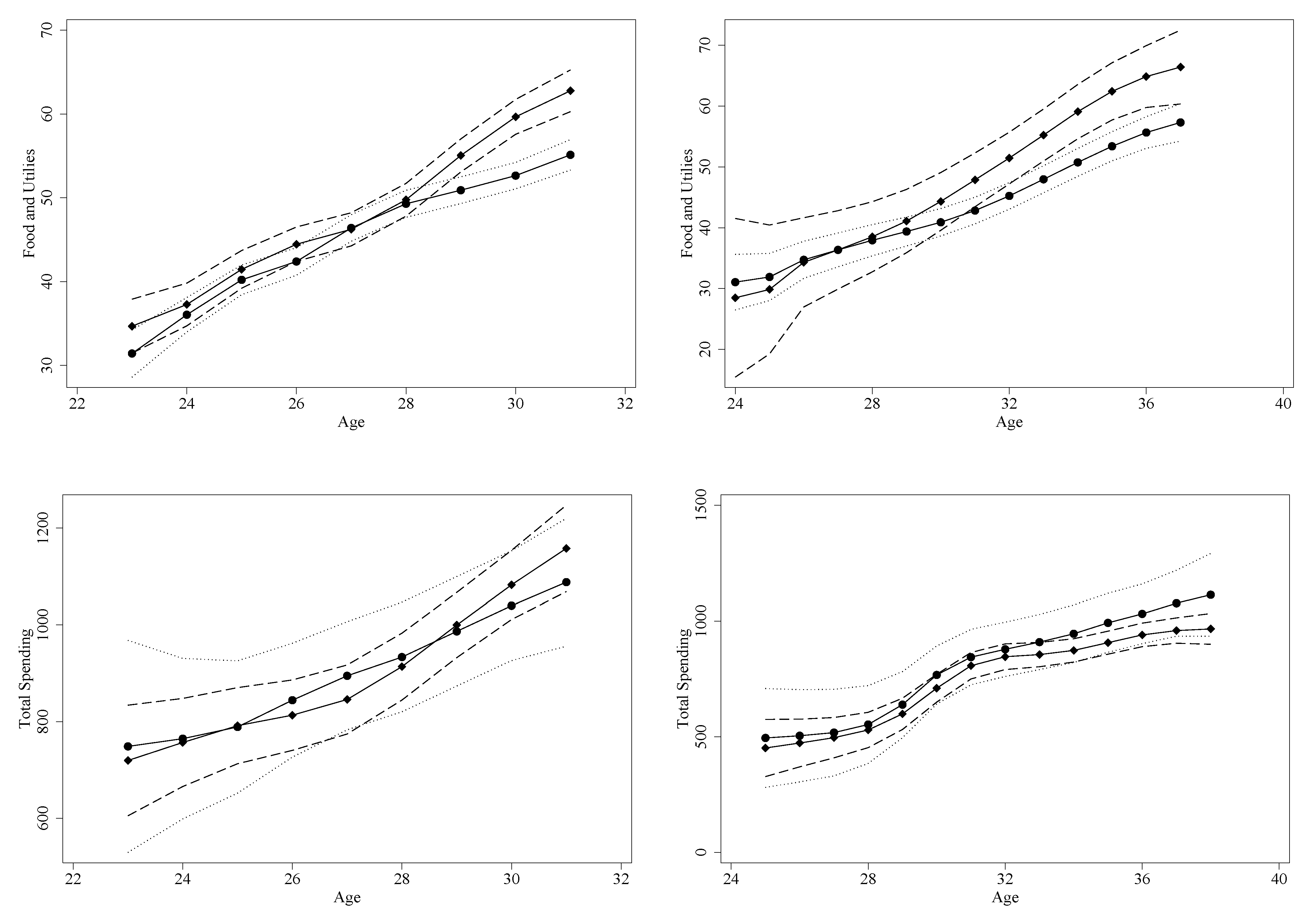
Before proceeding, let us compare some of the characteristics of the two groups of households. The top-right portion of Figure 8 shows the number of children that the later-born (or younger) cohort had in the years following the 1998 survey (estimated using a kernel regression that controls for education, race, and cohort), while the top-left picture shows the results for the earlier-born (or older) cohort. Households reporting that having children is important are plotted with diamond symbols, while if having children is not important, then circles are used instead. In both cases, a 95% significance region is plotted as a dashed line for those who report having children is important and as a dotted line if having children is not important. The figures show that, even though neither group had children when asked the question, both groups had children in the years that followed, but there were significant differences between the number of children that members of the two groups had, with those reporting having children is important significantly more likely to have children. This difference is particularly striking for the older cohort. These figures establish that the question is able to predict differences between the two groups in terms of children (the tests associated with these figures are reported in Table 3).
The kernel estimates of labour incomes for these two year-of-birth cohorts are also plotted in Figure 8. The figure shows that, for the younger cohort, there was no significant difference in the income of the two groups. For the older cohort, although there appeared to be a small difference at older ages, the difference was statistically insignificant. Overall, it seems that the income profiles were broadly similar. That is, those households for whom having children is important had a similar level of income as those households for whom having children is unimportant. Of course, we would like to establish that the level of income is the same for both groups over the whole life-cycle. However, this would require that we actually observe these two groups for their entire lives, which we cannot do in our panel. Nevertheless, we clearly established that (i) the two groups have similar income profiles, but (ii) they differ significantly in the number of children that they anticipate. Hence, if children affect the life-cycle pattern to consumption, these two groups should differ significantly in their consumption behaviour.
The level of consumption for these two groups is plotted in Figure 9. The top half of the figure looks at food consumption, while the bottom half looks at total spending. For both the younger and the older cohort, it shows that there was a significant difference between the two groups when looking at food and utilities consumption (top), but not for total spending (bottom). In both cases, food and utilities spending seem to diverge at older ages (when we established that these households had children). These pictures fully support the idea that children cause the hump-shape in life-cycle consumption if we concentrate on food and utilities consumption, but not when we look at total spending. Notice, indeed, that for the older cohort, while the difference in total spending was not significant (at the 5% significance level), there was a small gap between the two groups, but it was the households who did not anticipate children who increased their spending above those who did anticipate children. This is in direct contrast to what would be expected if households were inter-temporally substituting consumption from periods without children to periods in which they had children. That is, those households that want children (and we found were more likely to have children) should have higher consumption at the end of the period, not lower consumption.
4.3.2. The 2003 Wave
The response to the question about whether having children is important was also asked in the 2003 wave (there were around 350 households on average in each cohort-year cell for the younger cohort). The older cohort was excluded since the households were sufficiently old for few of these households to reasonably expect children. We know from the 1998 wave that this question predicts whether households that are currently childless will have children at some future date. Thus, while we did not look at the number of children in the household in the years following (2003 is near the end of the period for which we have data), we can compare the behaviour of childless households who responded that having children is important and those who do not believe it is important. The results are reported in Figure 10 (tests reported Table 4). The left half of the figure shows that there is no significant difference in labour income. The right half of Figure 10 looks at total spending prior to 2003, and hence during that part of the life-cycle where neither group has yet had children. Recall that the theory strongly predicts that the households who want children should be reducing their consumption when they are young if children explain the life-cycle pattern of consumption. However, Figure 10 shows again no difference in the behaviour of the two groups. Both types of households had remarkably similar consumption profiles over this part of the life-cycle.
4.4. With Whom an Individual Couples
So far, the analysis exploited responses to questions about the expectations of having children. Section 4.2 investigated households that self-reported that they expected to have children, while Section 4.3 investigated those households responding that having children is important. However, it is also possible to distinguish those households that, due to their type, are unlikely (or significantly less likely) to have children. As the data are a panel of households, it is possible to establish with whom an individual couples, or equivalently, with whom an individual forms a household (attention was restricted to individuals that are over 30 since it is common for there to be communal living among younger people prior to forming long-term relationships). Those households that are formed by two individuals of the same sex are, by construction, unlikely to have children, while those individuals that form opposite-sex couples are more likely to have children. This means that the consumption behaviour of these two groups can be compared. If children are causing the hump-shaped pattern to life-cycle consumption, then there should be a systematic difference between the behaviour of these two types of households: households formed by matching between individuals of the same sex and households formed by matching between individuals of the opposite sex. Testing for whether the two groups behave differently in regard to their consumption over the life-cycle is a test of the role of children in life-cycle consumption behaviour.
The paper thus constructed two groups on the basis of whether households are same-sex couples or opposite-sex couples. A household was classified as a same-sex household if there were two adults in the household of the same sex that either (i) declare themselves to be a couple or (ii) are over thirty, remain together for at least two years, and neither person in the couple ever forms a couple with someone of the opposite sex. Constructing same-sex and opposite-sex couples has the advantage that the analysis does not rely on the household’s response to an attitudinal survey. The drawback, however, is that relatively few households form same-sex couples (only around 3% of the 1200 couples included in the analysis each year). This necessitates changing the year-of-birth cohorts: the analysis now included only the older of the two cohorts with a slightly increased age range, so that it included those born between 1958 and 1968. This also means that the analysis in this section constructed estimates with fixed bandwidths and excluded the controls.
To start, it is useful, as in the previous sections, to see whether the income profiles are the same for both types of households. The left-hand side of Figure 11 (tested in Table 5) shows the labour income over the life-cycle for the two groups: same-sex couples are recorded with circles, while opposite-sex couples are recorded with diamonds. While there seems to be considerably more noise in the data for same-sex couples, both same-sex and opposite-sex households seem to have a similar pattern to their income as they age. The incomes were not significantly different, except at ages 33 and 34, where the same-sex households had a slightly lower income. The incomes of same-sex couples had previously been investigated by Black et al. (2007), who found, using the 2000 U.S. Census, that males who match with other males earn less than otherwise observationally equivalent men, but women who match with other women earn more than other women. This paper did not separate such households by sex; hence, the finding in this paper is in line with previous research.
Recall that if, as theory predicts, children cause consumption to increase in the middle of the life-cycle, then same-sex couples should be spending less in the middle of the life-cycle and more at the beginning of the life-cycle, compared to opposite-sex couples. That is, they should spend more at the beginning of the sample period and less at the end. Figure 11 plots consumption over the life-cycle for the two groups in the sample. It shows that the two consumption profiles seem to match each other extremely closely (Table 5 confirms this result). While spending by same-sex households was significantly lower at age 34, by the end, there spending was actually higher (although not statistically significant). This is in sharp contrast to what would be predicted if children were causing consumption to increase. In fact, the prediction would be that same-sex couples would be spending less at older ages and more at younger ages. This is clearly not observed in the data. It seems that the evidence here does not support the idea that children are causing the pattern of consumption that we observed for households over their life-cycle if households are moving consumption from childless periods to periods in which they have children.
5. Conclusions
The paper investigated the role of children in explaining the path of consumption (or household expenditure) over the life-cycle and, particularly, that consumption is higher in the middle of the life-cycle than either the beginning or the end of the life-cycle. That spending needs to increase when the household has children has been proposed as an explanation for this hump in life-cycle consumption. This explanation, at its simplest, predicts that households need to consume more when children are in the household compared to when they are not present, in order for the marginal utility of consumption to be held constant. If children explain the life-cycle profile of consumption observed when the average consumption for each year-of-birth cohort is plotted against age, then there should be systematic differences between households that plan to have children and households that do not. Those households that do not plan to have children have no need to save when young in order that they can increase the level of consumption when they are older and have children. Thus, contrasting the behaviour of different types of households (according to whether they anticipate children) is a natural experiment, which tests the theory that children explain life-cycle consumption. This test is independent of the role that any other explanation of the life-cycle pattern of consumption might play, such as risk-aversion, credit constraints, or myopia.
Using the BHPS, the paper determined those currently childless households that are likely to have children in the future in several different ways. First, households were directly asked whether they expected to have children at some future date. Second, households were asked about whether having children is important. Third, households were partitioned according to whether they formed couples of the same sex or of the opposite sex. In each case, the behaviour of the different groups was compared. The paper found that those who reported that they expected to have children were genuinely more likely to have children before the end of the survey period, as were households that reported that having children is important, but for the most part, there were no systematic differences in income between the groups.4
If children explain the hump in life-cycle consumption, then households that anticipate having children should consume less before children arrive, and more after they arrive. However, for the younger cohort, the results showed that there was no significant difference in the pattern of total spending for households expecting children either in 1992 or in 1998. For the older cohort, those asked in 1992 whether they expected children had lower total consumption in two of the years before children arrived. Those asked the question in 1998 showed higher consumption in the two years at then end of the sample, but these were years in which the household’s income was also higher. For households reporting that having children is important in 1998, while there were significant differences in the consumption of food and utilities, there were no differences in total spending (which uses a broader definition of consumption). Results for wanting children in 2003, and for same-sex matching, also showed that consumption is not significantly different in that part of the life-cycle which is observed in the survey.
Overall, the results do not seem to offer much support to the idea that there is a significant difference in the spending behaviour of those who anticipate children compared to those who do not. This finding is puzzling if family composition is genuinely causing the hump-shaped pattern to consumption over the life-cycle, but it seems robust to several different attempts to assess the theory. It seems unlikely that this result is because the data were too poor to be able to distinguish the level of consumption (or rather expenditure) of the different groups. As the paper showed, the data can demonstrate the hump-shaped profile to consumption (in Section 2). Moreover, some regressions did indeed show that there was a difference in spending between the two groups when attention was restricted to food and utilities spending (or for total spending in later years in Figure 5, when income also differed between the two groups). The overall picture that emerges from this study is that the hump-shaped pattern of consumption over the life-cycle does not seem to be caused by households formulating lifetime consumption plans in full anticipation of the arrival of children, since differences in whether households anticipated children were not clearly associated with differences in the consumption behaviour of these households. Thus, these results suggest that the hump-shaped pattern to consumption remains a puzzle.
Some further remarks are necessary. The aim of the paper was to investigate the role of children in explaining the hump shape to life-cycle consumption (plotted in Figure 1). The simplest way that children can cause this hump is through treating children as exogenous taste-shifters that cause households to move consumption from periods without children to periods with children. It is this formulation of the theory that was tested. Of course, it may still be the case that children are important when thinking about consumption behaviour: they undoubtedly heavily influence the composition of spending (food and utilities spending seem to be higher after children arrive, at least for those households reporting that having children is important). More subtly, households may change a whole raft of behaviours after the arrival of children. For instance, children may well affect the trade-off between work and leisure (or more generally, the use of time). This could mean that rather than substituting consumption over time (which was tested in this paper), households instead raise both spending and income (by working more hours or by delaying retirement) and do this several years after the arrival of children: while this study found there is no significant difference in income, it only observed households up to early middle age. Hence, the precise role of children in consumption behaviour remains an open issue. Nevertheless, this paper seemed to demonstrate that children can not be treated as exogenous taste-shifters that cause households to move consumption between different periods during the early part of the life-cycle: households anticipating children do not reduce their consumption prior to the children’s arrival or raise their consumption immediately afterwards.
Funding
This research received no external funding.
Data Availability Statement
The data is publicly available from the UK Data Service, and is fully described at this website: https://www.iser.essex.ac.uk/bhps/acquiring-the-data (10 November 2021).
Conflicts of Interest
The author declares that there are no conflict of interest.
Appendix A. Additional Supporting Material
The figures in the main body of the text display the results of kernel estimates of income, children, and consumption. This section estimates some simpler regressions, adding some more results. The results were estimated in a simpler way: by constructing the prediction for each year-type combination.5 The results reported in this section also omit the demographic controls from the regression. Immediately below is a discussion of the individual tables, but the broad picture is similar to that in the main text: the results do not seem to offer much support for the hypothesis that the hump in life-cycle consumption can be explained by children, since those who did not anticipate children did not have a significantly different life-cycle consumption profile.
Expecting children in 1992: The results without controls and for the fixed bandwidth for expecting children in 1992 are shown in Table A1. The results were similar, but not exactly the same, as those discussed in the main body of the text. For the younger cohort, households who expected children were now significantly more likely to actually have children before the end of the sample period. Food and utility consumption was again higher at the beginning of the sample, but as before, total spending did not differ between those who expected children and those who did not. For the older cohort, those who expected children were more likely to have children, but their income was now significantly higher by the end of the sample period. These households had higher spending on food and utilities, but there total spending was no higher than the group who did not expect children in 1992.
Expecting children in 1998: Table A2 reports results for households who expected children in 1998. These results show that for both the younger and the older cohort, if the household expected to have children, then they were genuinely more likely to have children. However, for both cohorts, they were also likely to have higher income (although only right at the beginning of the sample period for the younger cohort). For the younger cohort, there was no significant difference in the level of consumption each year between those who expected children and those who did not. For the older cohort, both food and utilities spending and total spending were significantly higher in most periods for the group who expected children. However, this does not strongly support the hypothesis that households shift consumption to periods in which they have children since the consumption is higher even in periods before the children arrive. A simpler explanation, in this particular case, is that the group who expected children had higher consumption because they had a higher income.
Wanting children in 1998: The comparison between those for whom children were important and those for whom it was not, excluding the controls, is reported in Table A3. It shows that wanting children (e.g., those who reported that having children is important), for both cohorts, resulted in the household being significantly more likely to have children by the last sample period. For the younger cohort, there was no difference in the income levels for the two groups. For the older cohort, the income differences were insignificant except briefly in the middle of the sample period where households wanting children had a lower income. For both cohorts, food and utilities consumption were higher at the end of the sample period, which is in line with the theory that children explain the hump in life-cycle consumption. Total spending for the younger cohort was also higher in the last few years (after children have arrived), but was lower for the older cohort. Having lower spending after the children arrive directly contradicts and rejects the theory that children cause the life-cycle consumption hump.
Wanting children in 2003: Results without controls for wanting children in 2003 are reported in Table A4. The results are the same as those reported in the main text, since they show that households for whom having children was important had the same level of income as those for whom it was not important. Both groups also had the same level of overall spending. Recall that we were looking at the period before the children arrived; thus, if children cause the hump in life-cycle consumption, we should observe those who reported that children was important had lower consumption in the sample period. Hence, the results do not seem to support the theory.

Table A1.
Comparing households expecting/not expecting future children in 1992.
| Age | 24 | 25 | 26 | 27 | 28 | 29 | 30 | 31 | |
| Cohort 0: Children | |||||||||
| Difference | −0.01 | 0.03 | 0.05 | 0.06 | 0.06 | 0.10 | 0.15 * | 0.19 * | |
| (0.05) | (0.05) | (0.06) | (0.06) | (0.06) | (0.06) | (0.07) | (0.08) | ||
| Income | |||||||||
| Difference | 215 | 123 | 86 | 251 * | 361 ** | 245 | 96 | −56 | |
| (174) | (151) | (149) | (108) | (117) | (134) | (145) | (190) | ||
| Food Consumption | |||||||||
| Difference | 5.38 ** | 4.62 ** | 3.63 * | 3.06 | 2.95 | 2.80 | 3.78 | 4.31 | |
| (1.61) | (1.61) | (1.74) | (1.75) | (1.83) | (2.17) | (2.37) | (3.11) | ||
| Total Consumption | |||||||||
| Difference | 24 | 16 | 8 | 4 | 39 | 67 | 73 | 57 | |
| (36) | (35) | (37) | (42) | (46) | (50) | (59) | (78) | ||
| Age | 30 | 31 | 32 | 33 | 34 | 35 | 36 | 37 | 38 |
| Cohort 1: Children | |||||||||
| Difference | 0.07 | 0.05 | 0.05 | 0.09 | 0.19 ** | 0.29 ** | 0.37 ** | 0.44 ** | 0.50 ** |
| (0.06) | (0.05) | (0.06) | (0.07) | (0.07) | (0.07) | (0.07) | (0.07) | (0.08) | |
| Income | |||||||||
| Difference | 89 | 98 | 122 | 141 | 194 | 259 * | 378 ** | 348 ** | 379 * |
| (122) | (109) | (112) | (116) | (120) | (126) | (138) | (141) | (177) | |
| Food Consumption | |||||||||
| Difference | 2.45 | 0.16 | 1.91 | 2.45 | 6.25 ** | 7.19 ** | 8.58 ** | 9.25 ** | 9.40 ** |
| (1.79) | (1.77) | (1.77) | (1.91) | (1.88) | (1.99) | (2.05) | (2.29) | (2.99) | |
| Total Consumption | |||||||||
| Difference | −91 | −69 | −7 | 20 | −1 | 11 | −8 | 42 | 15 |
| (76) | (52) | (46) | (44) | (45) | (46) | (49) | (54) | (69) | |
Notes: How much more is earned/consumed by households not expecting children compared to households wanting children. Throughout the table, * significant at 5%, ** significant at 1%.
Table A2.
Comparing households expecting/not expecting future children in 1998.
| Age | 24 | 25 | 26 | 27 | 28 | 29 | 30 | 31 | |||||||
| Cohort 0: Children | |||||||||||||||
| Difference | 0.07 * | 0.12 ** | 0.16 ** | 0.17 ** | 0.17 ** | ||||||||||
| (0.03) | (0.03) | (0.04) | (0.04) | (0.06) | |||||||||||
| Income | |||||||||||||||
| Difference | 487 ** | 420 ** | 278 | 133 | −130 | −6 | 45 | 230 | |||||||
| (137) | (137) | (153) | (158) | (167) | (188) | (203) | (269) | ||||||||
| Food Consumption | |||||||||||||||
| Difference | 2.41 | 2.14 | −0.03 | −0.10 | −2.23 | −1.03 | −1.34 | −0.70 | |||||||
| (2.20) | (2.37) | (2.55) | (2.71) | (2.69) | (2.72) | (2.89) | (3.69) | ||||||||
| Total Consumption | |||||||||||||||
| Difference | 60 | 64 | −9 | −24 | −82 | −3 | 29 | 96 | |||||||
| (46) | (47) | (63) | (70) | (82) | (79) | (85) | (109) | ||||||||
| Age | 25 | 26 | 27 | 28 | 29 | 30 | 31 | 32 | 33 | 34 | 35 | 36 | 37 | 38 | |
| Cohort 1: Children | |||||||||||||||
| Difference | 0.11 ** | 0.19 ** | 0.28 ** | 0.33 ** | 0.36 ** | ||||||||||
| (0.03) | (0.03) | (0.03) | (0.03) | (0.04) | |||||||||||
| Income | |||||||||||||||
| Difference | 7 | 32 | 113 | 204 * | 286 * | 432 ** | 540 ** | 579 ** | 728 ** | 899 ** | 1114 ** | 1170 ** | 1200 ** | 1145 ** | |
| (88) | (87) | (96) | (103) | (114) | (110) | (115) | (128) | (128) | (132) | (129) | (167) | (170) | (225) | ||
| Food Consumption | |||||||||||||||
| Difference | 0.97 | 1.15 | 2.38 | 4.41 ** | 5.92 ** | 6.92 ** | 6.74 ** | 5.33 ** | 4.32 * | 5.53 * | 7.71 ** | 10.13 ** | 11.01 ** | 10.97 ** | |
| (1.45) | (1.42) | (1.47) | (1.60) | (1.71) | (1.72) | (1.77) | (1.86) | (2.12) | (2.25) | (2.40) | (2.63) | (3.08) | (4.13) | ||
| Total Consumption | |||||||||||||||
| Difference | 55 * | 32 | 39 | 52 * | 83 * | 130 ** | 195 ** | 178 ** | 119 * | 123 * | 155 ** | 249 ** | 300 ** | 385 ** | |
| (23) | (23) | (23) | (23) | (36) | (42) | (46) | (49) | (52) | (52) | (53) | (54) | (59) | (78) | ||
How much more is earned/consumed by households not expecting children compared to households expecting children. Throughout the table, * significant at 5%, ** significant at 1%.
Table A3.
Comparing households wanting/not wanting children in 1998.
| Age | 24 | 25 | 26 | 27 | 28 | 29 | 30 | 31 | |||||||
| Cohort 0: Children | |||||||||||||||
| Difference | 0.03 | 0.12 ** | 0.19 ** | 0.27 ** | 0.30 ** | 0.37 ** | 0.41 ** | 0.44 ** | |||||||
| (0.02) | (0.03) | (0.03) | (0.03) | (0.04) | (0.04) | (0.05) | (0.06) | ||||||||
| Income | |||||||||||||||
| Difference | 173 | 170 | 103 | 102 | 113 | 98 | 112 | 95 | |||||||
| (118) | (97) | (101) | (95) | (102) | (106) | (108) | (135) | ||||||||
| Food Consumption | |||||||||||||||
| Difference | 1.53 | 2.91 * | 1.76 | 1.01 | 0.41 | 3.42 * | 6.05 ** | 7.29 ** | |||||||
| (1.45) | (1.37) | (1.37) | (1.38) | (1.55) | (1.68) | (1.80) | (2.21) | ||||||||
| Total Consumption | |||||||||||||||
| Difference | 0 | 8 | −20 | −31 | 7 | 67 | 119 * | 159 * | |||||||
| (33) | (32) | (31) | (34) | (42) | (45) | (52) | (67) | ||||||||
| Age | 25 | 26 | 27 | 28 | 29 | 30 | 31) | 32 | 33 | 34 | 35 | 36 | 37 | 38 | |
| Cohort 1: Children | |||||||||||||||
| Difference | −0.03 | 0.20 ** | 0.41 ** | 0.56 ** | 0.63 ** | 0.64 ** | 0.61 ** | 0.59 ** | |||||||
| (0.02) | (0.04) | (0.05) | (0.05) | (0.06) | (0.05) | (0.06) | (0.07) | ||||||||
| Income | |||||||||||||||
| Difference | −6 | 76 | 129 | 121 | 169 | 215 | 174 | −42 | −286 ** | −423 ** | −406 ** | −208 | −285 | −261 | |
| (102) | (105) | (105) | (101) | (118) | (113) | (112) | (100) | (102) | (109) | (117) | (160) | (162) | (217) | ||
| Food Consumption | |||||||||||||||
| Difference | 0.00 | 1.62 | 1.93 | 1.78 | 1.33 | 2.36 | 3.50 * | 5.33 ** | 6.73 ** | 7.59 ** | −9.03 ** | 10.18 ** | 10.28 ** | 9.99 ** | |
| (1.60) | (1.55) | (1.49) | (1.44) | (1.37) | (1.34) | (1.40) | (1.49) | (1.65) | (1.76) | (1.92) | (2.06) | (2.31) | (2.97) | ||
| Total Consumption | |||||||||||||||
| Difference | 19 | 9 | 4 | −3 | 49 | 17 | 4 | 35 | −8 | −56 | −74 | −93 * | −116 * | −177 ** | |
| (28) | (25) | (26) | (28) | (36) | (44) | (44) | (45) | (43) | (42) | (42) | (45) | (49) | (63) | ||
How much more is earned/consumed by households not wanting children compared to households wanting children. Throughout the table, * significant at 5%, ** significant at 1%.
Table A4.
Comparing households wanting/not wanting children in 2003.
| Age | 23 | 24 | 25 | 26 | 27 | 28 |
| Wave | 7 | 8 | 9 | 10 | 11 | 12 |
| Cohort 0: Income | ||||||
| Difference | −98 | −156 | −190 | −162 | 20 | 96 |
| (146) | (125) | (107) | (100) | (91) | (110) | |
| Food Consumption | ||||||
| Difference | 23 | 22 | −47 | −31 | −9 | 28 |
| (69) | (47) | (39) | (36) | (36) | (44) | |
How much more is earned/consumed by households not wanting children compared to households wanting children. Throughout the table, * significant at 5%, ** significant at 1%.
| 1 | Clearly, if households are credit constrained, they will not be able to adjust their behaviour whether or not they anticipate children. In such cases, we would expect no observable differences between households who do and who do not anticipate children. If this is the case, the hump in household consumption would not be caused by children. |
| 2 | Both Chok (2017) and Ejrnaes and Jorgensen (2020) looked at how fertility risk affects consumption behaviour. These papers argued that abortion allows households to reduce their family size as a result of negative income shocks. |
| 3 | Ignoring for measurement error in the construction of consumption, the left-hand side variable will make it easier to find significant results, since it is likely to under-estimate the true error bounds around the estimates. |
| 4 | Although Chok (2017) and Ejrnaes and Jorgensen (2020) both argued that households abort a pregnancy when faced with negative income shocks, this paper did not find significant income differences; this is likely to be because this paper did not look at the number of children, but only whether there was at least one child. |
| 5 | To be precise, the results construct a simple average for a 3 y bandwidth (e.g., the average of observations for the previous year, that year, and the following year.). |
References
- Aguiar, Mark, and Erik Hurst. 2005. Consumption versus Expenditure. Journal of Political Economy 113: 919–48. [Google Scholar] [CrossRef] [Green Version]
- Aguiar, Mark, and Erik Hurst. 2007. Life-cycle Prices and Production. American Economic Review 97: 1533–59. [Google Scholar] [CrossRef] [Green Version]
- Attanasio, Orazio, James Banks, Costas Meghir, and Guglielmo Weber. 1999. Humps and Bumps in Lifetime Consumption. Journal of Business and Economic Statistics 17: 22–35. [Google Scholar]
- Banks, James, Richard Blundell, and Sarah Tanner. 1998. Is there a Retirement-Savings Puzzle. American Economic Review 89: 902–20. [Google Scholar]
- Black, Dan, Seth Sanders, and Lowell Taylor. 2007. The Economics of Gay and Lesbian Families. Journal of Economic Perspectives 21: 53–70. [Google Scholar] [CrossRef] [Green Version]
- Blundell, Richard, Martin Browning, and Costas Meghir. 1994. Consumer Demand and Life-Cycle Allocation of Household Expenditures. Review of Economic Studies 61: 57–80. [Google Scholar] [CrossRef]
- Browning, Martin, and Mette Ejrnaes. 2009. Consumption and children. Review of Economics and Statistics 91: 93–111. [Google Scholar] [CrossRef] [Green Version]
- Browning, Martin, and Tim Crossley. 2001. The Life-Cycle Model of Consumption and Saving. Journal of Economic Perspectives 15: 3–22. [Google Scholar] [CrossRef] [Green Version]
- Browning, Martin, Angus Deaton, and Margaret Irish. 1985. A Profitable Approach to Labor Supply and Commodity Demands over the Life Cycle. Econometrica 53: 503–44. [Google Scholar] [CrossRef]
- Carroll, Christopher. 1997. Buffer-Stock Saving and the Life-Cycle/ Permanent Income Hypothesis. Quarterly Journal of Economics 112: 1–56. [Google Scholar] [CrossRef]
- Carroll, Christopher, and Lawrence Summers. 1991. Consumption Growth Parrallels Income Growth: Some New Evidence. In National Saving and Economic Performance. Edited by B. Douglas Bernheim and John B. Shoven. Chicago: Chicago University Press, pp. 305–43. [Google Scholar]
- Chok, Sekyu. 2017. Fertility Risk in the life-cycle. International Economic Review 58: 237–59. [Google Scholar]
- Deaton, Angus. 1991. Saving and Liquidity Constraints. Econometrica 59: 1221–48. [Google Scholar] [CrossRef]
- Ejrnaes, Mette, and Thomas Jorgensen. 2020. Family Planning in a life-cycle model with income risk. Journal of Applied Econometrics 35: 567–86. [Google Scholar] [CrossRef]
- Fernandez-Villaverde, Jesus, and Dirk Kreuger. 2007. Consumption Over the Life Cycle: Facts from the Consumer Expenditure Survey. Review of Economics and Statistics 89: 552–65. [Google Scholar] [CrossRef] [Green Version]
- Fernandez-Villaverde, Jesus, and Dirk Kreuger. 2011. Consumption Over the Life Cycle: How Important are Consumer Durables. Macroeconomic Dynamics 15: 725–70. [Google Scholar] [CrossRef] [Green Version]
- Gourinchas, Pierre-Olivier, and Jonathan Parker. 2002. Consumption Over the Life Cycle. Econometrica 70: 47–89. [Google Scholar] [CrossRef] [Green Version]
- Irvine, Ian. 1978. Pitfalls in the Estimation of Optimal Lifetime Consumption Patterns. Oxford Economic Papers 30: 301–9. [Google Scholar] [CrossRef]
- Jorgensen, Thomas. 2017. Life-cycle Consumption and Children: Evidence from a Structural Estimation. Oxford Bulletin of Economics and Statistics 79: 717–46. [Google Scholar] [CrossRef] [Green Version]
- Kraft, Holger, Claus Munk, Frank Seifried, and Sebastian Wagner Wagner. 2017. Consumption Habits and Humps. Economic Theory 64: 305–30. [Google Scholar] [CrossRef] [Green Version]
- McLanahan, Sara. 2004. Diverging Destinies: How Children are Faring under the Second Demographic Transition. Demography 41: 607–27. [Google Scholar] [CrossRef]
- Park, Hyeon. 2012. Present Biased Preferences and the Constrained Consumer. University of Pittsburgh Working Paper. [Google Scholar]
- Skinner, Jonathan. 1998. Risky income, life cycle consumption, and precautionary savings. Journal of Monetary Economics 22: 237–55. [Google Scholar] [CrossRef] [Green Version]
- Taylor, Marcia, and John Brice. 1999. British Household Panel Survey User Manual: Introduction, Technical Reports, and Appendices. ESRC Research Centreon Micro-Social Change. Colchester: University of Essex. [Google Scholar]
- Thurow, Lester. 1969. The Optimum Lifetime Distribution of Consumption Expenditures. American Economic Review 59: 324–30. [Google Scholar]
Figure 1.
Labour income/children and consumption over the lifecycle. Notes: The top half of the figure plots average real monthly income and consumption for each year and each year-of-birth cohort. Income is plotted with a solid line, while consumption is plotted with a dashed line. The bottom half of the figure plots the number of children and consumption for each year and each year-of-birth cohort. Children are plotted with a solid line, while consumption is plotted with a dashed line. In each case, the left panel plots food consumption, while the right panel plots total spending.

Figure 2.
Having children and labour income by cohort. Notes: The figure shows kernel regressions for labour income for households born between 1971 and 1977 (left) and between 1964 and 1970 (right), with their median age reported on the horizontal axis. Households that eventually have children are plotted as diamonds, while households who do not have children are plotted as circles. Dashed lines represent 95% confidence intervals for households who have children, and dotted lines represent 95% confidence intervals for households who do not.

Figure 3.
Having children and food and utilities/total consumption by cohort. Notes: The figure shows kernel regressions for food and utilities consumption (top) and total spending (bottom) for households born between 1971 and 1977 (left) and between 1964 and 1970 (right), with their median age reported on the horizontal axis. Households that eventually have children are plotted as diamonds, while households who do not have children are plotted as circles. Dashed lines represent 95% confidence intervals for households who have children, and dotted lines represent 95% confidence intervals for households who do not.

Figure 4.
Expecting children in 1992 and actual children/labour income by cohort. Notes: The figure shows kernel regressions for the number of children (top) and labour income (bottom) for households born between 1971 and 1977 (left) and between 1964 and 1970 (right), with their median age reported on the horizontal axis. Households that expect children in 1992 are plotted with diamonds, while households not expecting children in 1992 are plotted with circles. Dashed lines represent 95% confidence intervals for households expecting children, and dotted lines represent 95% confidence intervals for households not expecting children.

Figure 5.
Expecting children in 1992 and food and utilities/total consumption by cohort. Notes: The figure shows kernel regressions for food and utilities consumption (top) and total spending (bottom) for household’ born between 1971 and 1977 (left) and between 1964 and 1970 (right), with their median age reported on the horizontal axis. Households that expect children in 1992 are plotted as diamonds, while households not expecting children in 1992 are plotted as circles. Dashed lines represent 95% confidence intervals for households expecting children, and dotted lines represent 95% confidence intervals for households not expecting children.

Figure 6.
Expecting children in 1998 and actual children/labour income by cohort. Notes: The figure shows the kernel regressions for the number of children (top) and labour income (bottom) for households born between 1971 and 1977 (left) and between 1964 and 1970 (right), with their median age reported on the horizontal axis for two different year-of-birth cohorts. Households that do not expect children in 1998 are plotted as circles, while households expecting children in 1998 are plotted as diamonds. Dashed lines represent 95% confidence intervals for households expecting children, and dotted lines represent 95% confidence intervals for households not expecting children.

Figure 7.
Expecting children in 1998 and food and utilities/total consumption by cohort. Notes: The figure shows kernel regressions for food and utilities consumption (top) and total spending (bottom) for households born between 1971 and 1977 (left) and between 1964 and 1970 (right), with their median age reported on the horizontal axis. Expecting children in 1998 is plotted as diamonds, while not expecting children in 1998 is plotted as circles. Dashed lines represent 95% confidence intervals for households expecting children, and dotted lines represent 95% confidence intervals for households not expecting children.

Figure 8.
Wanting children in 1998 and actual children/labour income by cohort. Notes: The figure shows kernel regressions for the number of children (top) and labour income (bottom) for households born between 1971 and 1977 (left) and between 1964 and 1970 (right), with their median age reported on the horizontal axis for two different year-of-birth cohorts. Households that reported “having children is important” in 1998 are plotted as diamonds, while those reporting “having children is not important” in 1998 are plotted as a circle. Dashed lines represent 95% confidence intervals for households wanting children, and dotted lines represent 95% confidence intervals for households not wanting children.

Figure 9.
Wanting children in 1998 and food and utilities/total consumption by cohort. Notes: The figure shows kernel regressions for food and utilities consumption (top) and total spending (bottom) for households born between 1971 and 1977 (left) and between 1964 and 1970 (right), with their median age reported on the horizontal axis. Households that reported “having children is important” in 1998 are plotted as diamonds, while those reporting “having children is not important” in 1998 are plotted as circles. Dashed lines represent 95% confidence intervals for households wanting children, and dotted lines represent 95% confidence intervals for households not wanting children.

Figure 10.
Wanting children in 2003 and labour income/total spending. Notes: The figure shows kernel regressions for labour income (left) and total spending (right) for households born between 1971 and 1977 with their median age reported on the horizontal axis. Households that reported “having children is important” in 2003 are plotted as diamonds, while those reporting “having children is not important” in 2003 are plotted as circles. Dashed lines represent 95% confidence intervals for households expecting children, and dotted lines represent 95% confidence intervals for households not expecting children.

Figure 11.
Same-/opposite-sex couples and labour income/total spending. Notes: The figure shows average labour income (left) and average total spending (right) for households born between 1958 and 1968with their median age reported on the horizontal axis. Same-sex couples are plotted with circles, while opposite-sex couples are plotted with diamonds. Dashed lines represent 95% confidence intervals.

Table 1.
Comparing households expecting/not expecting future children in 1992.
| Age | 24 | 25 | 26 | 27 | 28 | 29 | 30 | 31 | |
| Cohort 0: Children | |||||||||
| Difference | −0.010 | 0.003 | 0.015 | 0.029 | 0.049 | 0.076 | 0.134 | 0.160 | |
| (0.100) | (0.081) | (0.074) | (0.073) | (0.073) | (0.075) | (0.074) | (0.083) | ||
| Income | |||||||||
| Difference | 188 | 126 | 117 | 187 | 307 * | 275 | 151 | 124 | |
| (172) | (154) | (147) | (144) | (145) | (147) | (153) | (181) | ||
| Food Consumption | |||||||||
| Difference | 5.05 * | 5.44 * | 4.67 * | 3.30 | 2.25 | 2.53 | 4.16 | 5.71 * | |
| (2.44) | (2.15) | (2.02) | (1.97) | (1.99) | (2.04) | (2.16) | (2.57) | ||
| Total Consumption | |||||||||
| Difference | 43 | 64 | 54 | 21 | 29 | 61 | 81 | 92 | |
| (63) | (56) | (53) | (52) | (51) | (50) | (51) | (62) | ||
| Age | 30 | 31 | 32 | 33 | 34 | 35 | 36 | 37 | 38 |
| Cohort 1: Children | |||||||||
| Difference | 0.115 | 0.043 | 0.084 | 0.231 | 0.347 * | 0.378 * | 0.447 ** | 0.541 ** | |
| (0.176) | (0.166) | (0.165) | (0.165) | (0.166) | (0.164) | (0.164) | (0.186) | ||
| Income | |||||||||
| Difference | −111 | −51 | −1 | 14 | 30 | 92 | 198 | 279 * | 289 |
| (162) | (135) | (124) | (120) | (119) | (119) | (121) | (128) | (148) | |
| Food Consumption | |||||||||
| Difference | −2.81 | −2.51 | −1.68 | 0.31 | 2.46 | 3.87 | 5.05 * | 5.81 * | 5.90 |
| (3.50) | (2.86) | (2.61) | (2.53) | (2.51) | (2.52) | (2.56) | (2.72) | (3.19) | |
| Total Consumption | |||||||||
| Difference | −159 | −142 * | −125 * | −111 | −97 | −75 | −42 | −11 | 8 |
| (83) | (70) | (63) | (60) | (58) | (57) | (59) | (63) | (74) | |
Notes: How much more is earned/consumed by households expecting children compared to households not expecting children. Throughout the table, * significant at 5%, ** significant at 1%.
Table 2.
Comparing households expecting/not expecting future children in 1998.
| Age | 23 | 24 | 25 | 26 | 27 | 28 | 29 | 30 | 31 | |||||
| Cohort 0: Children | ||||||||||||||
| Difference | 0.109 | 0.135 | 0.234 | 0.245 | 0.180 | |||||||||
| (0.147) | (0.135) | (0.133) | (0.133) | (0.150) | ||||||||||
| Income | ||||||||||||||
| Difference | 345 | 269 | 187 | 99 | 23 | 20 | 123 | 304 | 471 | |||||
| (340) | (263) | (229) | (217) | (219) | (226) | (230) | (238) | (272) | ||||||
| Food Consumption | ||||||||||||||
| Difference | −5.53 | −5.75 | −5.34 | −4.77 | −4.12 | −2.95 | −1.23 | 0.807 | 1.95 | |||||
| (12.73) | (10.23) | (8.97) | (8.36) | (8.19) | (8.33) | (8.72) | (9.52) | (11.18) | ||||||
| Total Consumption | ||||||||||||||
| Difference | 19 | 8 | −8 | −40 | −77 | −68 | −12 | 41 | 75 | |||||
| (101) | (80) | (68) | (62) | (60) | (61) | (63) | (68) | (79) | ||||||
| Age | 25 | 26 | 27 | 28 | 29 | 30 | 31 | 32 | 33 | 34 | 35 | 36 | 37 | 38 |
| Cohort 1: Children | ||||||||||||||
| Difference | 0.224 | 0.319 * | 0.374 ** | 0.44 ** | 0.529 ** | |||||||||
| (0.141) | (0.145) | (0.141) | (0.141) | (0.153) | ||||||||||
| Income | ||||||||||||||
| Difference | −35 | 21 | 77 | 108 | 112 | 118 | 154 | 224 | 308 | 394 | 486 | 582 * | 667 * | 726 * |
| (262) | (241) | (234) | (237) | (246) | (256) | (264) | (269) | (272) | (274) | (277) | (286) | (307) | (350) | |
| Food Consumption | ||||||||||||||
| Difference | 2.89 | 3.99 | 4.73 | 4.98 | 4.56 | 3.50 | 1.98 | 0.52 | 0.14 | 1.12 | 3.13 | 5.81 | 8.32 | 9.92 |
| (5.71) | (5.00) | (4.68) | (4.55) | (4.51) | (4.52) | (4.57) | (4.67) | (4.84) | (5.08) | (5.36) | (5.72) | (6.34) | (7.59) | |
| Total Consumption | ||||||||||||||
| Difference | 53 | 44 | 43 | 30 | 42 | 120 | 157 * | 106 | 38 | 40 | 83 | 147 | 235 * | 288 * |
| (91) | (84) | (76) | (71) | (67) | (68) | (75) | (81) | (83) | (85) | (87) | (92) | (103) | (125) | |
Notes: How much more is earned/consumed by households not expecting children compared to households expecting children. Throughout the table, * significant at 5%, ** significant at 1%.
Table 3.
Comparing households for which children important/not important in 1998.
| Age | 24 | 25 | 26 | 27 | 28 | 29 | 30 | 31 | ||||||
| Cohort 0: Children | ||||||||||||||
| Difference | 0.147 | 0.255 ** | 0.245 ** | 0.360 ** | 0.397 ** | 0.488 ** | 0.475 ** | |||||||
| (0.087) | (0.074) | (0.071) | (0.071) | (0.070) | (0.070) | (0.078) | ||||||||
| Income | ||||||||||||||
| Difference | 153 | 156 | 71 | 4 | −3 | −27 | −30 | 39 | ||||||
| (110) | (96) | (89) | (86) | (85) | (85) | (87) | (102) | |||||||
| Food Consumption | ||||||||||||||
| Difference | 3.69 | 1.68 | 1.24 | 1.86 | 0.81 | 4.04 * | 6.61 ** | 7.08 ** | ||||||
| (2.70) | (2.07) | (1.81) | (1.67) | (1.59) | (1.60) | (1.67) | (1.98) | |||||||
| Total Consumption | ||||||||||||||
| Difference | −10 | −8 | −30 | −41 | −19 | 11 | 40 | 67 | ||||||
| (55) | (46) | (42) | (41) | (40) | (39) | (41) | (51) | |||||||
| Age | 25 | 26 | 27 | 28 | 29 | 30 | 31 | 32 | 33 | 34 | 35 | 36 | 37 | 38 |
| Cohort 1: Children | ||||||||||||||
| Difference | 0.290 | 0.450 ** | 0.587 ** | 0.640 ** | 0.633 ** | 0.644 ** | 0.620 ** | |||||||
| (0.104) | (0.090) | (0.090) | (0.092) | (0.092) | (0.092) | (0.101) | ||||||||
| Income | ||||||||||||||
| Difference | −124 | −92 | −70 | −56 | −31 | −1 | −10 | −87 | −204 | −301 | −343 | −348 | −359 | −391 |
| (574) | (490) | (438) | (398) | (365) | (339) | (321) | (312) | (310) | (314) | (319) | (326) | (346) | (402) | |
| Food Consumption | ||||||||||||||
| Difference | −2.04 | −1.13 | −0.40 | 0.01 | 0.59 | 1.73 | 3.44 | 5.07 * | 6.23 ** | 7.29 ** | 8.37 ** | 9.06 ** | 9.23 ** | 9.14 ** |
| (4.94) | (4.13) | (3.62) | (3.25) | (2.95) | (2.70) | (2.52) | (2.41) | (2.36) | (2.39) | (2.48) | (2.60) | (2.82) | (3.35) | |
| Total Consumption | ||||||||||||||
| Difference | −41 | −30 | −20 | −20 | −36 | −58 | −40 | −33 | −53 | −70 | −85 | −91 | −118 | −147 |
| (117) | (106) | (97) | (86) | (74) | (65) | (62) | (61) | (61) | (62) | (63) | (64) | (71) | (88) | |
Notes: How much more is earned/consumed by households wanting children in 1998 compared to households not wanting children. Throughout the table, * significant at 5%, ** significant at 1%.
Table 4.
Comparing households for which children important/not important in 2003.
| Age | 23 | 24 | 25 | 26 | 27 | 28 |
| Income | ||||||
| Difference | 138 | −110 | −165 | −114 | −37 | 58 |
| (159) | (122) | (103) | (91) | (86) | (97) | |
| Total Consumption | ||||||
| Difference | 65 | 13 | −21 | −32 | −16 | 4 |
| (71) | (56) | (47) | (43) | (43) | (49) |
Notes: How much more is earned/consumed by households wanting children in 2003 compared to households not wanting children. Throughout the table, * significant at 5%, ** significant at 1%.
Table 5.
Comparing same-sex and opposite-sex couples.
| Age | 30 | 31 | 32 | 33 | 34 | 35 | 36 | 37 | 38 | 39 | 40 | 41 |
| Income | ||||||||||||
| Difference | −42 | −8 | −203 | −329 * | −380 ** | −154 | −25 | −94 | −162 | −170 | −38 | 218 |
| (169) | (160) | (160) | (145) | (137) | (150) | (150) | (151) | (150) | (165) | (190) | (228) | |
| Total Consumption | ||||||||||||
| Difference | 15.27 | 27.75 | 6.85 | −43.08 | −91.33 * | −50.53 | −56.98 | −41.30 | −29.20 | −14.21 | −1.38 | 26.29 |
| (54.93) | (49.94) | (49.17) | (41.16) | (41.75) | (43.15) | (44.37) | (41.71) | (44.58) | (48.63) | (61.31) | (70.82) | |
Notes: How much more is earned/consumed by households wanting children in 2003 compared to households not wanting children. Throughout the table, * significant at 5%, ** significant at 1%.
Publisher’s Note: MDPI stays neutral with regard to jurisdictional claims in published maps and institutional affiliations. |
© 2022 by the author. Licensee MDPI, Basel, Switzerland. This article is an open access article distributed under the terms and conditions of the Creative Commons Attribution (CC BY) license (https://creativecommons.org/licenses/by/4.0/).
Share and Cite
MDPI and ACS Style
Grant, C. Children and Life-Cycle Consumption. J. Risk Financial Manag. 2022, 15, 42. https://doi.org/10.3390/jrfm15020042
AMA Style
Grant C. Children and Life-Cycle Consumption. Journal of Risk and Financial Management. 2022; 15(2):42. https://doi.org/10.3390/jrfm15020042
Chicago/Turabian StyleGrant, Charles. 2022. "Children and Life-Cycle Consumption" Journal of Risk and Financial Management 15, no. 2: 42. https://doi.org/10.3390/jrfm15020042