Compositional Classification of Financial Statement Profiles: The Weighted Case

Abstract

This article classifies petrol retail companies in Spain based on their financial ratios using the compositional data analysis (CoDA) methodology. This methodology solves the most common distributional problems encountered in the statistical analysis of financial ratios. The main purpose of this article is to show that with the CoDA methodology, accounting figures presenting low values can have a disproportional influence on classification. This problem can be attenuated by applying weighted CoDA, which is a novelty in the financial statement analysis field. The suggested weight of each accounting figure is proportional to its arithmetic mean. The results of Ward clustering show that after weighting, the contributions of the accounting figures to the total variance and to the clustering solution are more balanced, and the clusters are more interpretable. Four distinct financial profiles are identified and related to non-financial variables. Only one of the profiles represents companies in financial distress, with low turnover, low return on assets, high indebtedness, and low liquidity. Further developments include alternative weighting schemes.

1. Introduction

Financial ratios are commonly used as indicators of know how well a business is performing. They express the relationship between two or more accounting figures and allow researchers and professionals to analyze the solvency, liquidity, efficiency, and profitability of an individual company, and provide useful information to make better decisions, to de-risk investments, and to design sound financial policies (Chnar Abdullah 2021; Kacani et al. 2022; Qin et al. 2022; Shingade et al. 2022). Financial ratios pose no special problems for the analysis of single companies. However, when financial ratios are used as data in a statistical analysis of a sample of companies in an industry a number of serious problems appear, including redundancy, outliers, non-normality, non-linearity, skewness, and dependence of the results on which accounting figure is in the numerator or the denominator of the ratio (Linares-Mustarós et al. 2018). Using the compositional data analysis (CoDA) methodology reduces the extent of these problems and leads to obtaining more reliable conclusions from financial statement analysis at the industry level (Linares-Mustarós et al. 2018). CoDA applies logratio transformations to normalize the dataset so that the ulterior analysis is done with fewer outliers, with a more symmetric distribution, and with results that are invariant to permutation of the numerator and denominator of the ratio (Arimany-Serrat et al. 2022; Carreras-Simó and Coenders 2020, 2021; Creixans-Tenas et al. 2019; Linares-Mustarós et al. 2022; Saus-Sala et al. 2021).

The aim of this article is to classify companies according to the structure of their financial statements, in other words, clustering companies according to their financial ratios (Cowen and Hoffer 1982; Kalinová 2021). This has already been accomplished with CoDA methods (Linares-Mustarós et al. 2018; Saus-Sala et al. 2021). However, in compositional classification, it often happens that variables which generally take low values have the greatest variances and a disproportionate influence on the classification results (Greenacre 2018; Greenacre and Lewi 2009). In variables with low values, measurement errors also tend to have a greater impact (Hron et al. 2017), including the presence of zeros, which makes a lower influence desirable, not larger. For example, in the dataset used in this article, very low values, some of which equal to zero, are encountered in the non-current assets. These problems can be solved by giving weights to the variables. In this manner, the researcher can give less importance to the variables that would otherwise have a too large of an influence on the results (Egozcue and Pawlowsky-Glahn 2016; Hron et al. 2022). Weighing in compositional classification can be understood to play a similar role as standardization in other classification problems. It must be taken into account that, in compositional classification, variables cannot be standardized in the usual manner (Linares-Mustarós et al. 2018).

Drawing from a sample of companies in retail sales of automotive fuel in specialized stores, we present the classification results from both perspectives, weighted and unweighted. In this manner, the changes in the clusters of companies are highlighted depending on whether they are based on compositional distances computed from weighted or unweighted variables. To the best of our knowledge, this is the first scholarly article applying weights to a compositional financial statement analysis.

This article is structured as follows. Section 2 explains the basics of compositional data analysis and logratio transformations, the importance of weights, the dataset and software used, the selected financial ratios, the zero replacement and, finally, the clustering method. Section 3 shows the difference between the weighted and unweighted results on the sample data and the manner in which the weighted results are interpreted. Finally, Section 4 discusses the research findings and further implementations.

2. Materials and Methods

2.1. What Is Compositional Data Analysis?

Traditionally, the term compositional data has referred to non-negative data with the distinctive property that the sum of their values is a constant, usually 1 or 100%. It does not matter if the data are expressed in kilometers, mg/liter, or euros. The process of dividing a set of data by its total to obtain compositional values, which are proportions adding up to 1, is called closing the data or closure (Aitchison 1982). For example, the weight percent would refer to closed data, and mg/liter would refer to non-closed data.

Compositional data are normally used in fields such as chemistry, geology, medicine or biology, but it can also be useful in social science fields (Coenders and Ferrer-Rosell 2020). Egozcue and Pawlowsky-Glahn (2019) drop the requirement of fixed sum, and define compositional data simply as an array of strictly positive numbers for which ratios between them are considered to be relevant. Financial statement figures do not have a fixed sum but fulfill this definition to the letter.

The parts of a composition are called components, in our case, selected accounting figures corresponding to accounts or account categories in the financial statements. Parts are expressed as j, and the number of parts is J. The companies are expressed as i, and the sample size is I. So, the composition data matrix X (I × J) is:

$$X=\left(\begin{array}{ccc}{x}_{11}& \dots & x_{1J}\\ \dots & \dots & \dots \\ x_{I1}& \dots & x_{IJ}\end{array}\right)\mathrm{with} x_{ij} > 0 \mathrm{for} \mathrm{all} i,j.$$

(1)

The CoDA methodology fulfills three principles (Pawlowsky-Glahn et al. 2015):

• Scale invariance means that compositional data only carry relative information. So, proportional X matrices are equivalent, and any change in the scale of the dataset has no effect and produces compatible results.
• Sub compositional coherence means that the relationships among a subset of parts of a composition are the same as in the full composition.
• Permutation invariance means that the results do not depend on the order of the parts in a compositional dataset. The parts can be re-ordered across the whole dataset without affecting the results.

2.2. Logratio Transformations and Compositional Distances

The CoDA methodology applies some form of logratio transformation before using any univariate or multivariate statistical analysis, such as clustering (Barceló-Vidal and Martín-Fernández 2016).

The reason to apply a logratio transformation is that raw financial ratios have a number of problems with their statistical treatment:

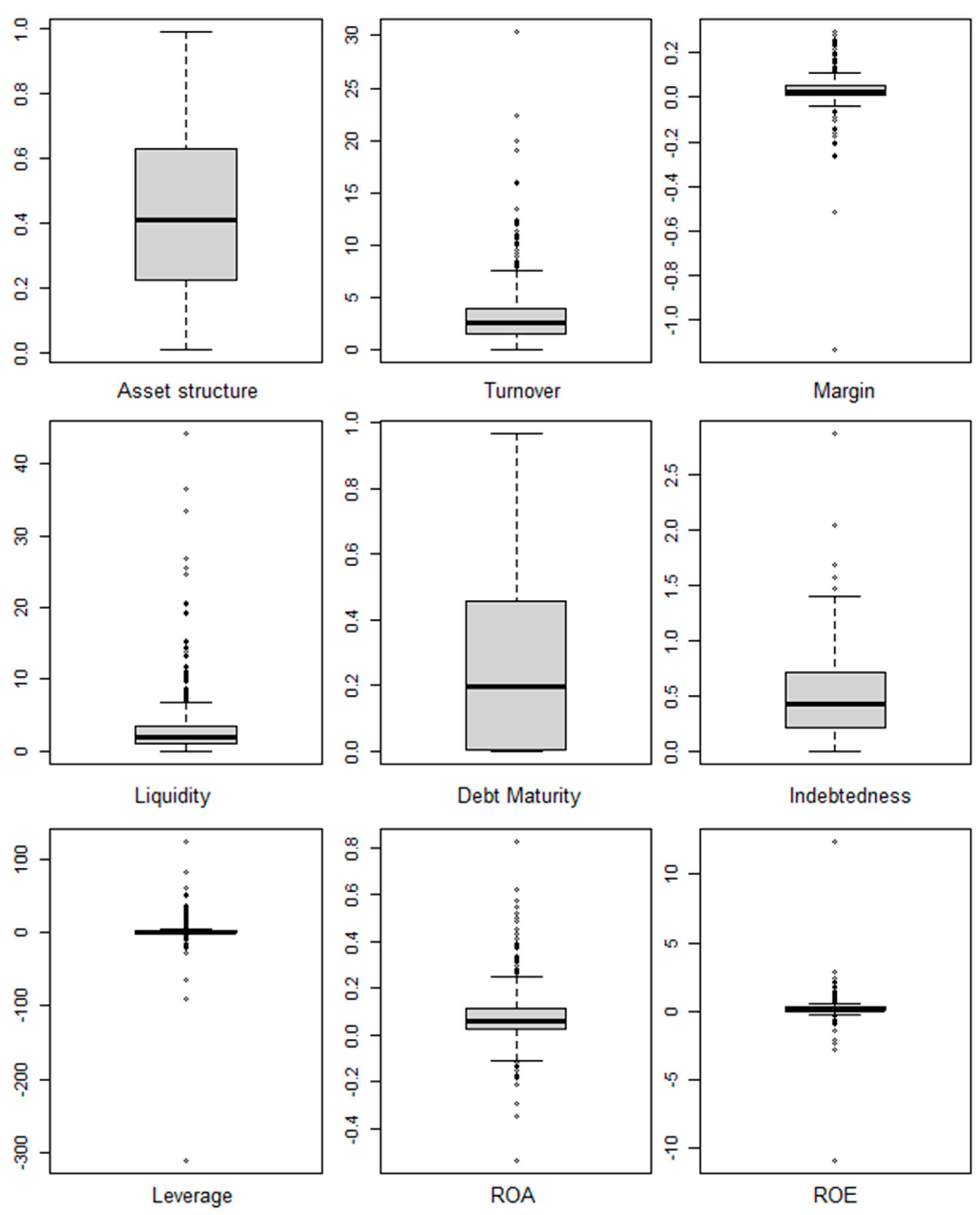
• Most of the ratios used in finance “are distributed between zero and infinity, and thus make fully symmetric distributions impossible to achieve” (Linares-Mustarós et al. 2018, p. 1). More particularly, they usually have positive skewness and outliers, thus deviating from the normal distribution (Linares-Mustarós et al. 2022; So 1987).
• The results of financial ratio analysis depend on the arbitrary decision regarding which accounting figure is in the numerator and which is in the denominator of the financial ratio, so that standard financial ratios are not permutation invariant (Creixans-Tenas et al. 2019; Frecka and Hopwood 1983; Linares-Mustarós et al. 2022).
• Financial statement analysis is subject to redundancy problems when several ratios conveying similar information are included in the dataset (Chen and Shimerda 1981). For example, the inverse of the liability-to-asset ratio is the equity-to-debt ratio plus one. In cluster analysis, such redundancy increases distances among companies along the added redundant information, which is tantamount to inadvertently giving this redundant information greater weight in the results (Linares-Mustarós et al. 2018).

Logratios solve the asymmetry, outlier, redundancy, and permutation dependence problems and are distributed between minus infinity and plus infinity, like the normal distribution (Linares-Mustarós et al. 2018).

Centered logratios (CLR) are the most common logratio transformation for compositional cluster analysis (Aitchison et al. 2000; Saus-Sala et al. 2021). “CLRs do not require choosing a reference part but refer each of the J parts to the geometric mean of all the parts” (Greenacre 2018, p. 18). The fact that only J logratios are computed prevents redundancy (Saus-Sala et al. 2021).

$$\mathrm{CLR}\left(x_{ij}\right)=\log \left(\frac{x_{ij}}{\sqrt[J]{x_{i1}{x}_{i2}\dots x_{iJ}}}\right).$$

(2)

When using CLR as data, Euclidean distances become equal to Aitchison compositional distances (Aitchison et al. 2000). The distance between company i and company i’ is:

$$\mathrm{D}\left(i,i^{\prime }\right)=\sqrt{{{\displaystyle \sum }}_{j=1}^J{\left(\mathrm{CLR}\left(x_{ij}\right)-\mathrm{CLR}\left(x_{i^{\prime }j}\right)\right)}^2.}$$

(3)

In this article, we apply weights to the components in order to decrease the influence of parts explaining a very large portion of total CLR variance (Hron et al. 2022). For this purpose, the weight of each part has to be decided. Greenacre (2018) and Greenacre and Lewi (2009) suggest that the weights applied on the parts (w_j), adding up to 1, should be the closed part means, because parts with low mean values also tend to dominate variance. For this reason, in this article, we are using weighted CLR (from here on WCLR):

$$\mathrm{WCLR}\left(x_{ij}\right)=\sqrt{w_j}\log \left(\frac{x_{ij}}{x_{i1}^{w1}{x}_{i2}^{w2}\dots x_{iJ}^{wJ}}\right) \mathrm{with} {\displaystyle \sum }_{j=1}^J{w}_j=1.$$

(4)

It must be taken into account that weights are applied to the columns of X (account categories in the financial statements), not the rows (companies). The weighted compositional distance between company i and company i’ is the Euclidean distance computed from WCLR (Greenacre and Lewi 2009):

$$\mathrm{WD}\left(i,i^{\prime }\right)=\sqrt{{{\displaystyle \sum }}_{j=1}^J{\left(\mathrm{WCLR}\left(x_{ij}\right)-\mathrm{WCLR}\left(x_{i^{\prime }j}\right)\right)}^2}.$$

(5)

The CLR and WCLR do not have a clear accounting interpretation. This issue is dealt with in Section 2.4, where it is shown that standard financial ratios can be used as supplementary variables for cluster interpretation. The CLR, WCLR, and distances used for compositional cluster analysis cannot be computed if some parts are zero for some of the companies. This issue is dealt with in Section 2.5, where it is shown how to impute zero values.

2.3. Dataset and Software

From here on, we compare the weighted and unweighted compositional classifications with a real-data example of the fuel station sector in Spain. Financial statements were obtained from the SABI (Iberian Balance Sheet Analysis System, accessible at https://sabi.bvdinfo.com/, accessed on 6 September 2022) database, developed by INFORMA D&B in collaboration with Bureau Van Dijk. Search criteria were NACE code 47.3 (retail sale of automotive fuel in specialized stores) in Spain with available data for 2021. The data include private and public limited companies with current assets, net sales, and costs above EUR 10,000 which had at least five employees (sample size I = 735).

All analyses were carried out with the R libraries zCompositions (Palarea-Albaladejo and Martín-Fernández 2015) for multivariate imputation of left-censored data, in other words, zero replacement, and easyCODA (Greenacre 2018) for univariate and multivariate methods for compositional data analysis based on logratios, including weighted and unweighted cluster analysis.

2.4. Selected Parts from the Balance Sheet and Profit and Losses Account and Financial Ratios

From the balance sheets and profit and losses accounts, we extracted the following non-negative parts:

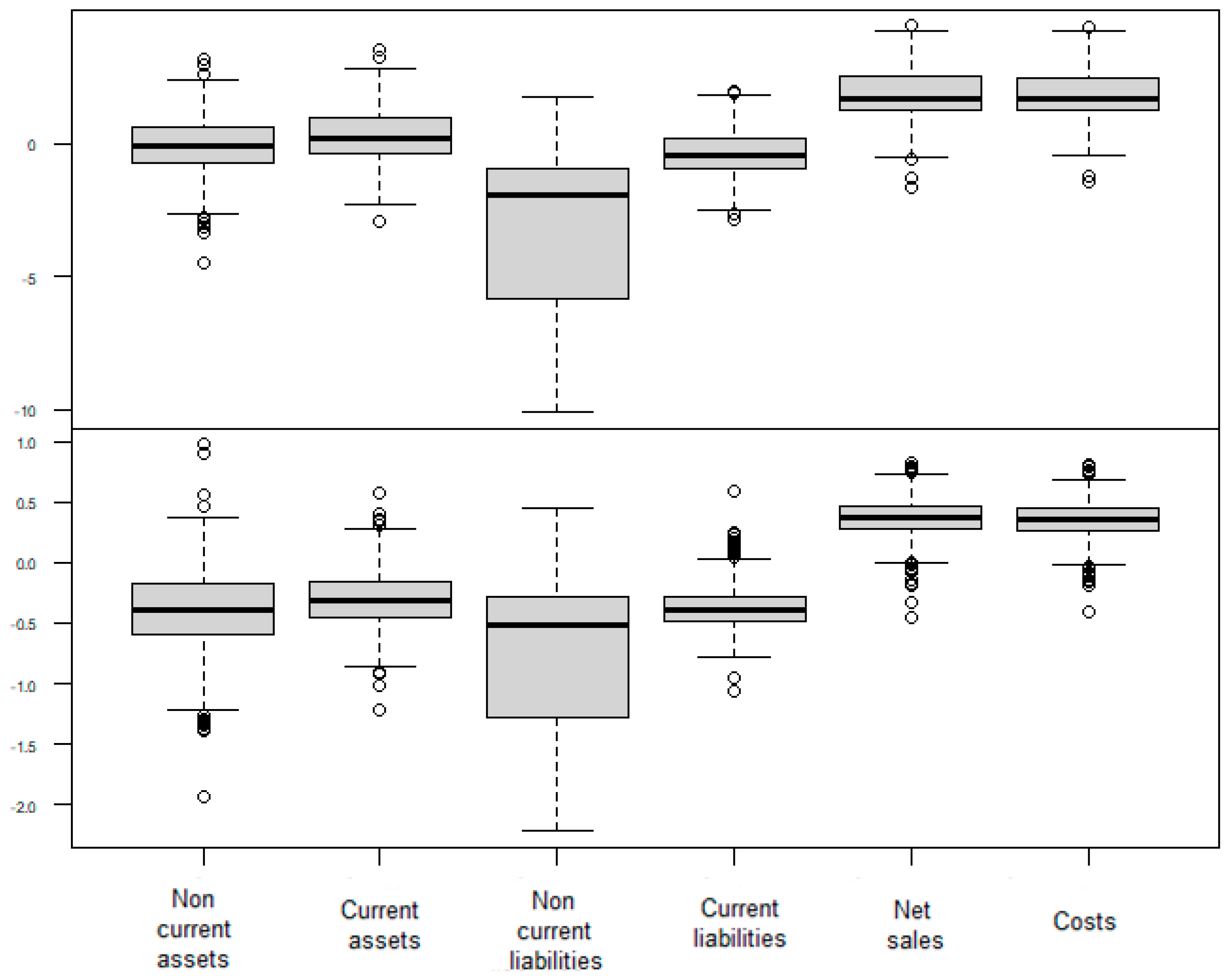
• x_i1 = non-current assets;
• x_i2 = current assets;
• x_i3 = non-current liabilities;
• x_i4 = current liabilities;
• x_i5 = net sales;
• x_i6 = costs.

The requirement for parts to be non-negative implies avoiding subtraction and using, for instance, current assets and current liabilities rather than working capital or using net sales and costs rather than operating profit (Creixans-Tenas et al. 2019). The selected parts are used for computing the CLR transformations and the distances, weighted and unweighted, and also for computing the standard financial ratios chosen by the researcher.

Even if weighted and unweighted cluster analyses are carried out from the CLR transformations or from the compositional distances (Coenders and Ferrer-Rosell 2020; Ferrer-Rosell and Coenders 2018; Greenacre 2018; Martín-Fernández et al. 1998), the clustering results can be interpreted from the standard financial ratios computed at cluster level, which are more familiar to researchers in accounting and finance than financial ratios constructed as CLR (Saus-Sala et al. 2021). These are the standard financial ratios that we used for the cluster interpretation:

• The turnover ratio measures the efficiency of a company assets in generating revenues:

  $$\frac{x_{\mathrm{i}5}}{x_{\mathrm{i}1}+x_{\mathrm{i}2}}.$$

  (6)
• The margin ratio measures the part of sales that is turned into profit:

  $$\frac{x_{\mathrm{i}5}-x_{\mathrm{i}6}}{x_{\mathrm{i}5}}.$$

  (7)
• The asset-structure ratio measures the share of non-current assets in total assets:

  $$\frac{x_{i1}}{x_{i1}{+x}_{i2}}.$$

  (8)
• The liquidity ratio compares current assets and current liabilities:

  $$\frac{x_{\mathrm{i}2}}{x_{\mathrm{i}4}}.$$

  (9)
• The debt-maturity ratio measures the share of non-current liabilities within total liability:

  $$\frac{x_{\mathrm{i}3}}{x_{\mathrm{i}3}+x_{\mathrm{i}4}}.$$

  (10)
• The indebtedness ratio measures the share of assets paid for by debt:

  $$\frac{x_{\mathrm{i}3}+x_{\mathrm{i}4}}{x_{\mathrm{i}1}+x_{\mathrm{i}2}}.$$

  (11)
• The leverage ratio relates assets to net worth:

  $$\frac{x_{\mathrm{i}1}+x_{\mathrm{i}2}}{\left(x_{\mathrm{i}1}+x_{\mathrm{i}2}\right)-\left(x_{\mathrm{i}3}+x_{\mathrm{i}4}\right)}.$$

  (12)
• The Return On Assets (ROA) divides the company’s net income by its total assets:

  $$\frac{x_{\mathrm{i}5}-x_{\mathrm{i}6}}{x_{\mathrm{i}1}+x_{\mathrm{i}2}}.$$

  (13)
• The Return On Equity (ROE) divides the company’s net income by net worth:

  $$\frac{x_{\mathrm{i}5}-x_{\mathrm{i}6}}{\left(x_{\mathrm{i}1}+x_{\mathrm{i}2}\right)-\left(x_{\mathrm{i}3}+x_{\mathrm{i}4}\right)}.$$

  (14)

Since standard financial ratios in Equations (6)–(14) do not participate in building the classification, their outliers, skewness, permutation, or redundancy (indebtedness and leverage are actually redundant) do not affect the classification results.

2.5. Zero Replacement

In order to compute logratios, it is required to first replace zero values, also called non-detects or values below detection limit (BDL), see Martín-Fernández et al. (2011).

Some early zero-replacement approaches like the non-parametric methods (Martín-Fernández et al. 2003) can bias the variance structure when the number of zeros is large. For this reason, the replacement method that we used is the well-known Expectation Maximization (EM) algorithm for missing data imputation adapted for compositional zero replacement (Palarea-Albaladejo and Martín-Fernández 2008).

This technique restores the dataset into a rectangular complete-data format by replacing each zero value with an imputed value BDL. Once the replacement is done, the logratios and distances can be computed for analysis (Palarea-Albaladejo and Martín-Fernández 2008).

In our dataset, there were 23.8% of zeros in non-current liabilities. The remaining parts of the financial statements had no zeros to replace. The detection limit for the EM algorithm was set at the minimum observed non-current-liability value which was EUR 202.

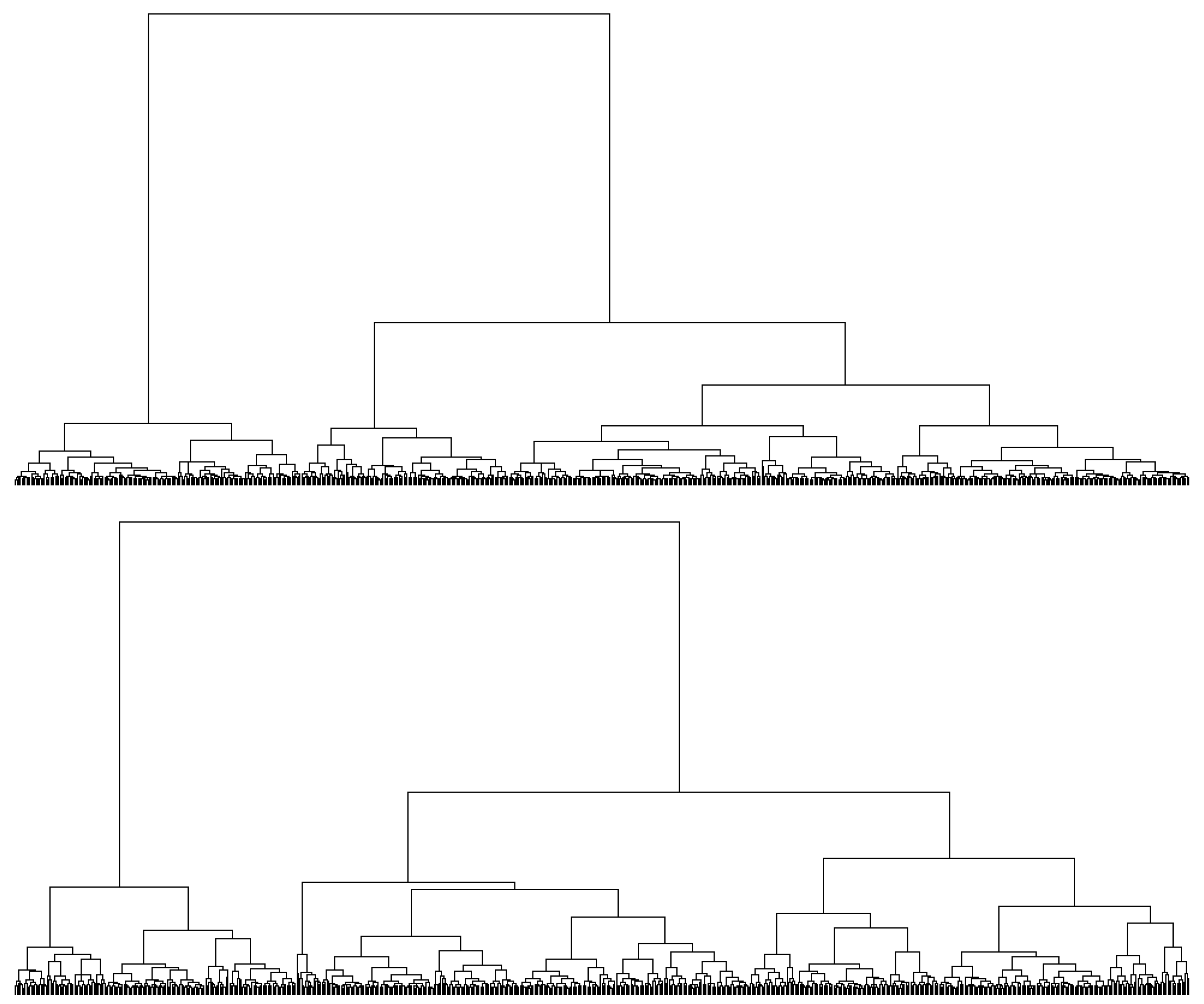
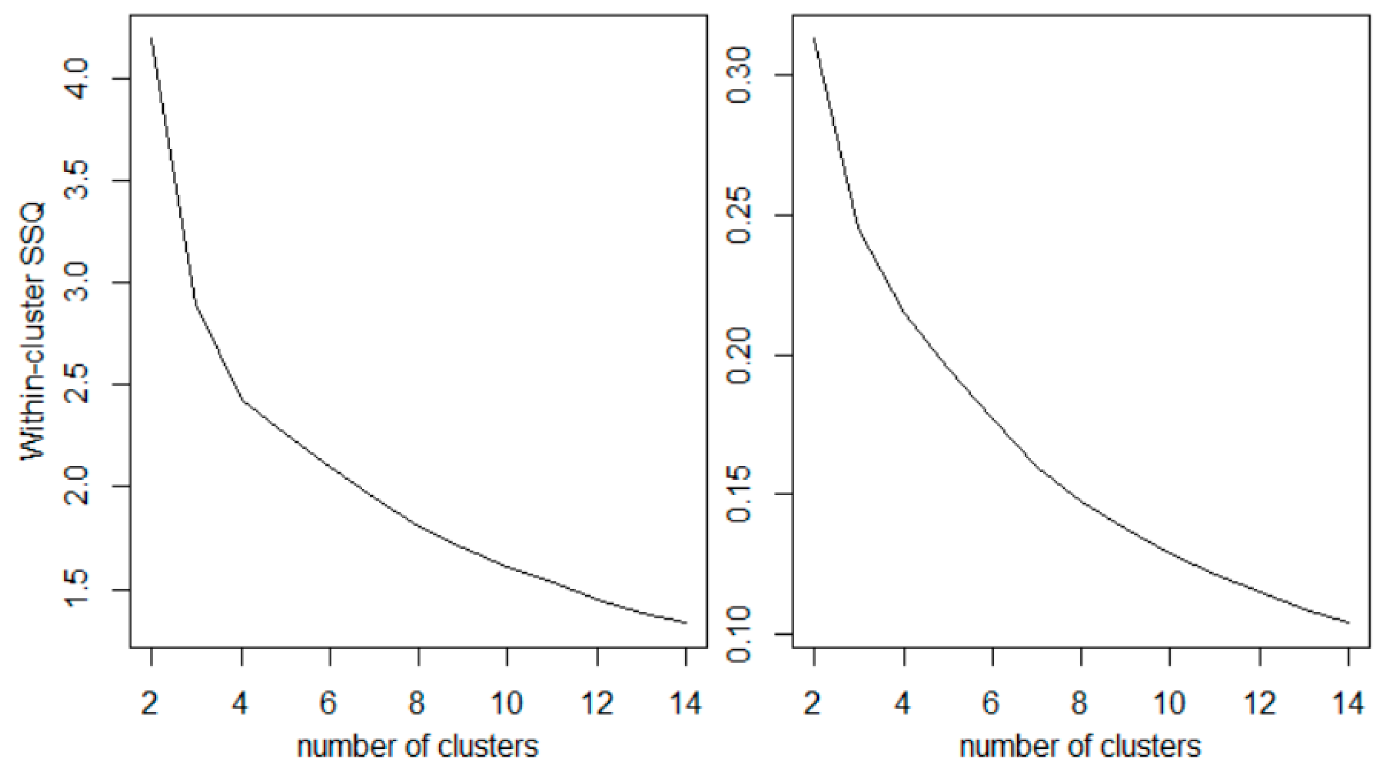
2.6. Cluster Analysis

As with any other data, with compositional data it is possible to perform a cluster analysis to classify individual compositions (in our case, companies) into groups of compositions. These groups contain companies that have low mutual weighted or unweighted Aitchison distances, and high distances with respect to companies in other groups (Greenacre 2018). Groups can thus be interpreted as distinct financial profiles (Linares-Mustarós et al. 2018).

We used the Ward clustering algorithm twice on the weighted and unweighted distances. The Ward method is one of the most popular clustering methods for financial ratios (Linares-Mustarós et al. 2018; Lukáč et al. 2021). For the purpose of comparing the results with and without weights, we computed the percentage of CLR variance explained by the classification in an Analysis of Variance (ANOVA) model.

We next computed the mean standard financial ratios for each cluster. For this purpose, the geometric means of all companies for each part are computed within each cluster of size C (Saus-Sala et al. 2021). It must be noted that here geometric means are computed column-wise, while in Equation (2) they are computed row-wise. For part j:

$$g\left(x_{.j}\right)=\sqrt[C]{x_{1j}{x}_{2j}\dots x_{Cj}}.$$

(15)

The geometric mean has the attractive property that the ratio of two geometric means equals the geometric mean of the ratios. For instance, the mean liquidity ratio (Equation (9)) for a given cluster is:

$$g\left(\frac{x_{.2}}{x_{.4}}\right)=\frac{g\left(x_{.2}\right)}{g\left(x_{.4}\right)}.$$

(16)

This property makes it possible to identify the typical financial statement profiles of each cluster in terms of standard ratios. The arithmetic mean does not have this property. First computing arithmetic means at the cluster level and then standard financial ratios between those means may stand in contradiction with the results of first computing standard ratios at firm level and then the cluster arithmetic means of those ratios (Saus-Sala et al. 2021).

Finally, we related the classification to the non-financial variables: company age, number of employees, company type (private or public limited company), and region (called autonomous community in Spain). Relationships with qualitative variables were assessed by means of χ² tests and mosaic plots (Dolnicar et al. 2018). Relationships with numeric variables were assessed by ANOVA F tests and confidence-interval plots. Following Goldstein and Healy (1995), when intervals drawn with 83% confidence do not overlap, there is a significant mean difference at α = 0.05.

3. Results

3.1. Exploratory Analysis

Figure 1 shows the boxplots of standard financial ratios, some of which show very extreme outliers (especially in turnover, margin, liquidity, leverage, ROA and ROE) and marked asymmetry (especially in turnover, liquidity, and indebtedness).

Figure 2 shows the importance of the transformations on the financial statements. We can observe how the outliers and skewness in both the CLR and WCLR transformations have been greatly reduced, which makes them much more appropriate as variables in a cluster analysis. Note that non-current liabilities stand out for a lower median.

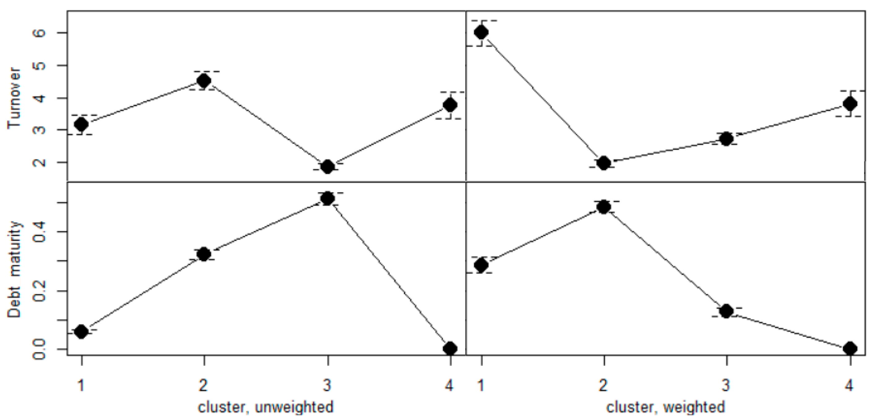
3.2. Comparison of Weighted and Unweighted Analysis

This section shows the importance of applying weights from different points of view.

Table 1. Closed arithmetic part means acting as weights.

Non-current assets	0.090
Current assets	0.096
Non-current liabilities	0.028
Current liabilities	0.051
Net sales	0.373
Costs	0.362

shows that non-current liabilities have by far the lowest mean. Accordingly, they dominate the CLR variance, accounting for over 71% (left column in

Table 2. Contributions of the parts to total CLR total variance (%) labelled according to the accounting figure in the numerator. Unweighted and weighted.

	Unweighted	Weighted
Non-current assets	7.1	17.4
Current assets	6.8	7.7
Non-current liabilities	71.2	63.4
Current liabilities	4.2	4.4
Net sales	5.3	3.5
Costs	5.4	3.6

). When we apply the weighted analysis with the part means in Table 1 as weights, we observe that the contributions to the total variance change. In our case, the contribution of non-current liabilities decreases as intended, from 71.2% to 63.4%, that of non-current assets increases, and the others remain almost at the same values (right column in Table 2).

Figure 3 presents the cluster analysis dendrograms. The upper dendrogram represents the unweighted classification, and the lower dendrogram the weighted classification. The lengths of the vertical lines represent distances at which two clusters are merged. When they are comparatively large, they suggest to stop merging the clusters. The unweighted dendrogram thus suggests a four-group solution. This is confirmed by the scree plot of within-cluster sums of squares in Figure 4, as recommended by Dolnicar et al. (2018). The point at which one sees an “elbow” shape shows the appropriate number of clusters, since to continue merging would imply a large jump in the sum of squares. For the weighted solution, between seven and three clusters seem to be appropriate according to the scree plot, and the four-group solution is selected for comparability purposes.

Table 3. Crosstabulation of the unweighted (columns) and weighted (rows) 4-cluster classifications.

	Cluster 1	Cluster 2	Cluster 3	Cluster 4	Total
Cluster 1	29	89	0	0	118
Cluster 2	4	42	238	0	284
Cluster 3	94	52	5	6	157
Cluster 4	3	0	0	173	176
Total	130	183	243	179

shows that weighting is not a statistical refinement, but can produce substantially different results for the classification. When we take a look at Clusters 1 and 2 we can see that the companies both change greatly after weighting. Cluster 3 stays more stable, and for the most (238 cases), corresponds to Cluster 2 after weighting. Cluster 4 does not present any relevant change, with 173 cases belonging to Cluster 4 in both classifications and only 6 + 3 = 9 cases shifting groups.

Table 4. Proportion of CLR variance explained by the weighted and unweighted classifications in an ANOVA model.

	Unweighted	Weighted
Non-current assets	0.35	0.43
Current assets	0.64	0.60
Non-current liabilities	0.95	0.91
Current liabilities	0.43	0.37
Net sales	0.73	0.76
Costs	0.73	0.76

shows that non-current liabilities dominate the proportion of CLR variance explained by the unweighted classification in an ANOVA model. This proportion decreases as intended when we apply weights, and higher values are obtained for non-current assets, net sales, and costs. Once more, the decision whether to weight or not to weight reveals itself as important. The proportion of unexplained variance for non-current liabilities nearly doubles, from 0.05 to 0.09.

Table 5. Cluster centers: standard financial ratios computed from cluster geometric means. Unweighted analysis.

	Cluster 1 17.7%	Cluster 2 24.9%	Cluster 3 33.1%	Cluster 4 24.4%
Turnover	2.77	4.32	1.61	3.08
Margin	0.04	0.03	0.04	0.03
Asset structure	0.37	0.27	0.65	0.28
Liquidity	2.70	1.97	1.28	2.99
Debt maturity	0.03	0.30	0.52	0.00
Indebtedness	0.24	0.53	0.57	0.24
Leverage	1.32	2.13	2.33	1.32
ROA	0.11	0.11	0.06	0.09
ROE	0.15	0.24	0.14	0.12

and

Table 6. Cluster centers: standard financial ratios computed from cluster geometric means. Weighted analysis.

	Cluster 1 16.1%	Cluster 2 38.6%	Cluster 3 21.4%	Cluster 4 23.9%
Turnover	5.69	1.77	2.45	3.18
Margin	0.02	0.04	0.03	0.03
Asset structure	0.16	0.60	0.45	0.28
Liquidity	2.09	1.34	2.41	3.12
Debt maturity	0.20	0.48	0.06	0.00
Indebtedness	0.50	0.57	0.24	0.23
Leverage	2.01	2.32	1.32	1.30
ROA	0.12	0.06	0.09	0.11
ROE	0.24	0.15	0.11	0.14

show the typical standard financial ratios for each cluster computed from the geometric means as described in Section 2.6 and will be interpreted in Section 3.3.

Table 7. Maximum difference between cluster centers in weighted and unweighted cluster analysis.

	Unweighted	Weighted
Turnover	2.704	3.920
Margin	0.014	0.014
Asset structure	0.379	0.441
Liquidity	1.709	1.782
Debt maturity	0.515	0.481
Indebtedness	0.329	0.339
Leverage	1.009	1.024
ROA	0.056	0.058
ROE	0.126	0.129

shows the range of these mean standard ratios, in other words, the maximum difference in the mean standard ratios for any two clusters. Table 7 once more shows how important weights applied on financial statement analysis are. When we apply weights to the parts, we can see that there are lower differences among clusters in the ratio in which non-current liabilities are involved (debt maturity). On the other hand, the remaining ratios have more pronounced differences in their cluster centers, or at least equal, after weighting.

Figure 5 provides added details on two ratios with particularly large differences before and after weighting: turnover and debt maturity. Weighting makes it possible to distinguish a high-turnover cluster which did not emerge in the unweighted solution. Before weighting, two clusters had very high debt maturity and two had very low debt maturity, intermediate profiles being absent. Note that the confidence intervals in Figure 5 cannot be used to test the significance of differences, because both the clusters and the ratios have been obtained from the same financial statement figures. This usage of confidence interval plots is reserved for Section 3.3.

In conclusion, with the results in this section we can corroborate the importance of weighting. When we apply weights, the results change substantially. We can see how non-current liabilities decrease their influence on the classification results, and we can thus obtain better balanced profiles in the cluster analysis. From here on we base our interpretation on the weighted solution.

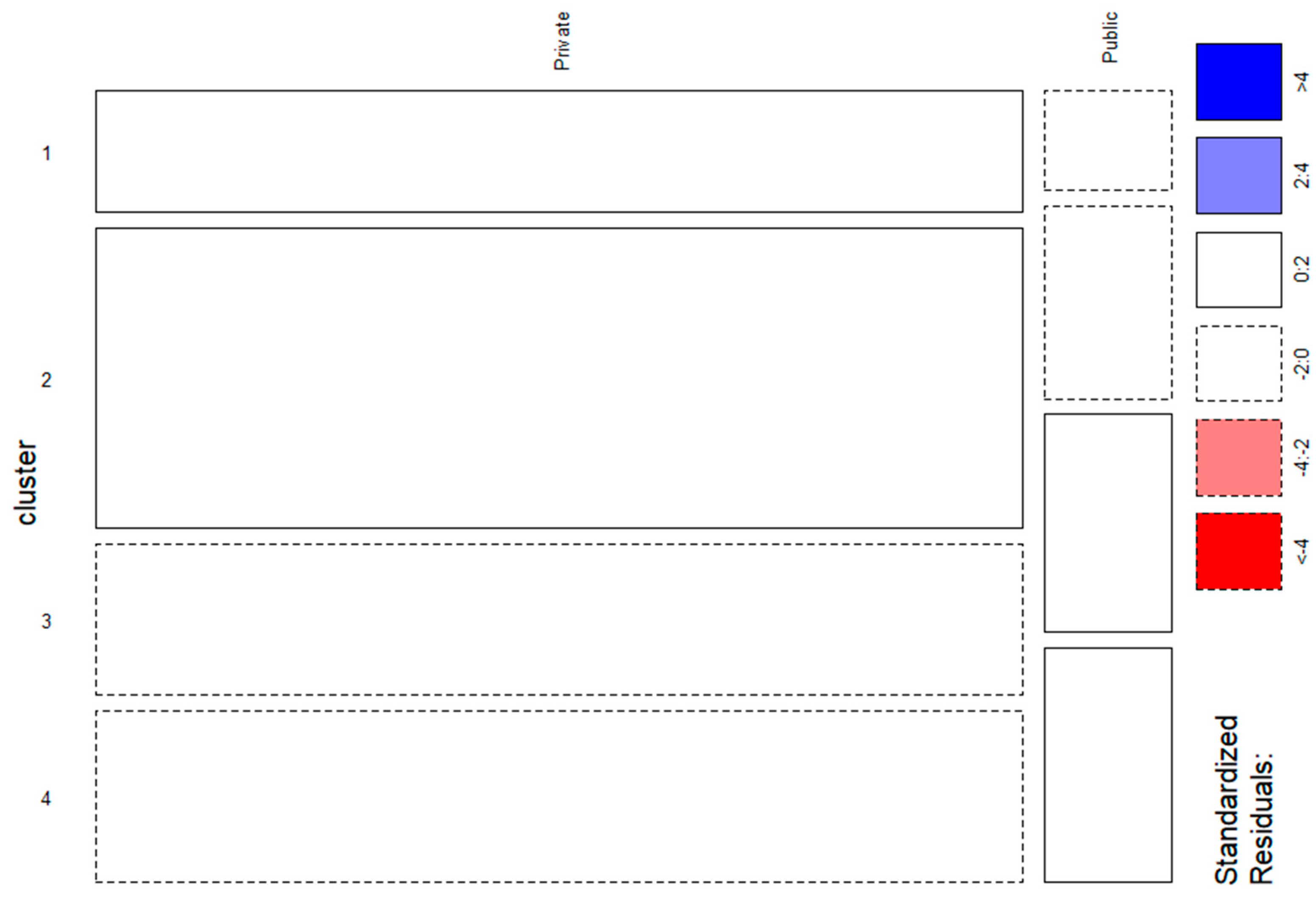
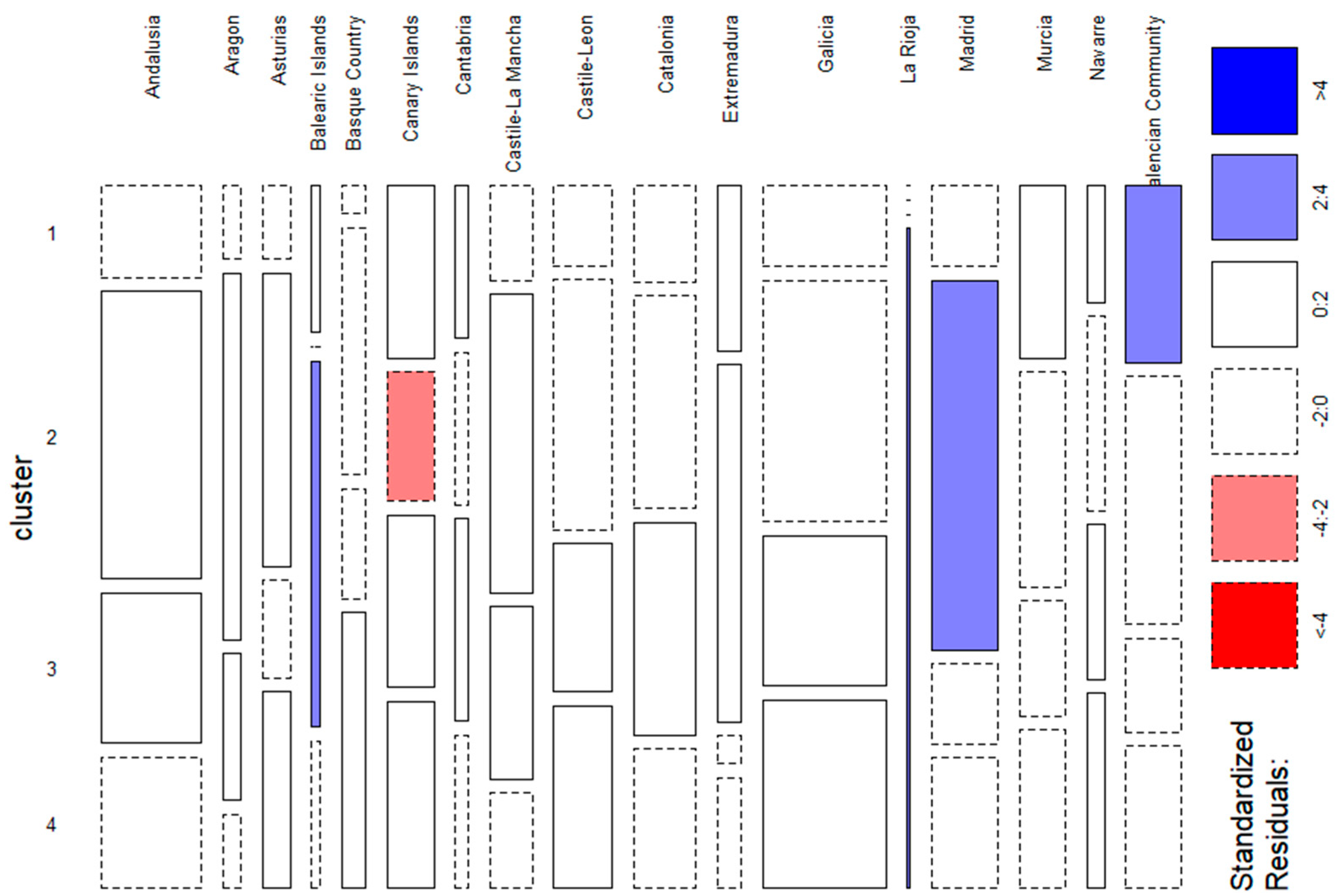
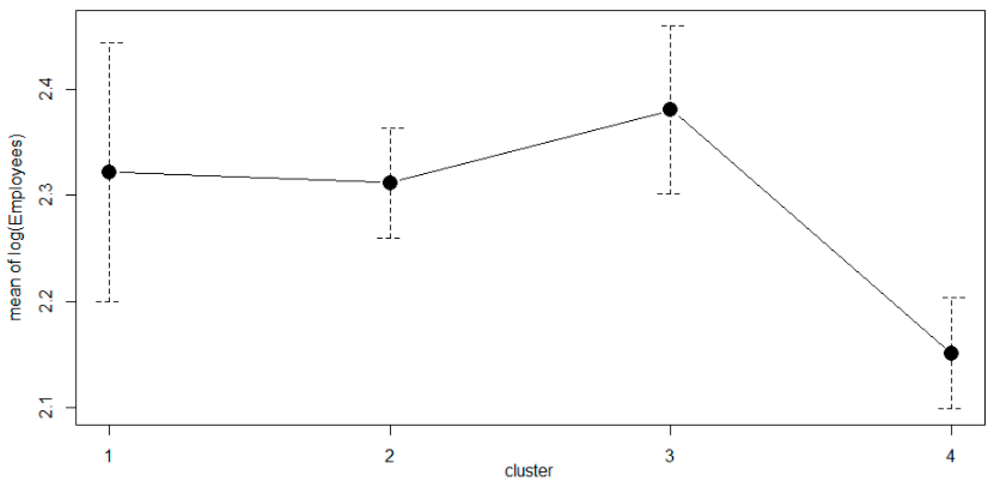
3.3. Interpretation of the Weighted Analysis

Table 6 presents the following cluster profiles. Cluster 1 has the highest turnover, the lowest margin, the lowest share of non-current assets in the asset structure, and the highest ROA and ROE. Cluster 2 has the lowest turnover, the highest margin, the highest share of non-current assets in the asset structure, the lowest liquidity, the highest debt maturity, the highest indebtedness and leverage, and the lowest ROA. Cluster 3 has the second to lowest indebtedness and leverage and the lowest ROE. Finally, Cluster 4 has the highest liquidity, the lowest debt maturity, and the lowest indebtedness and leverage.

To recap, Cluster 1 gathers the companies with the highest profitability, and cluster 2 gathers the companies that are the least profitable and have the lowest solvency, both at the short term (liquidity) and the long term (indebtedness). We can observe that Cluster 3 has intermediate performances and low indebtedness, and Cluster 4 contains the companies with the highest liquidity and with the lowest long-term debts.

The following paragraphs focus on the relationship between the cluster solution and each of the non-financial variables: company type, autonomous community, number of employees, and company age. All of them are statistically significant according to the χ² or F tests. The relationship with company type presents a p-value of 0.018, autonomous community a p-value of 0.007, employees a p-value of 0.016, and company age a p-value lower than 0.001.

In Figure 6, we can observe that Clusters 1 and 2 mainly contain private limited companies, while Clusters 3 and 4 are the ones that contain the most public limited companies.

If we concentrate on the cells with the highest standardized residuals in absolute value, in Figure 7 we can observe that the Valencia Community has the most companies in Cluster 1. Other remarkable cases are Madrid, which has the most companies gathered in Cluster 2, the Balearic Islands which has the most companies in Cluster 3, and La Rioja with nearly all companies in Cluster 4. The Canary Islands have the least companies in Cluster 2.

In Figure 8, we can observe that the mean number of employees of Clusters 1 and 2 are similar, while Cluster 3 has the highest mean and Cluster 4 the lowest. There are significant differences between Cluster 4 and Cluster 2 and between Cluster 4 and Cluster 3 whose confidence intervals do not overlap.

In Figure 9, we can observe that Cluster 1 presents the lowest mean company age, and Cluster 4 the highest, followed closely by Cluster 3. There are significant differences between Cluster 1 and Clusters 3 and 4, and between Cluster 2 and Clusters 3 and 4, because their confidence intervals do not overlap.

4. Discussion

This article puts forward a procedure to construct financial statement profiles by means of compositional cluster analysis. Outliers and skewness in standard financial ratios are treated by means of a CLR transformation (Saus-Sala et al. 2021). The CLR transformation is crucial for financial-statement clustering. If we cluster the companies based on standard financial ratios (Equations (6)–(14)), the four-group solution contains three groups with only outliers (cluster sizes are 727, 5, 2, and 1 companies).

The disadvantage of this approach is that financial statement figures with low values can have a disproportionate influence in the classification results. To solve this problem, for the first time, we use weights on the financial statement figures, so that we can give parts with low values a lower influence on the classification. Following the proposal by Greenacre (2018) and Greenacre and Lewi (2009), we use the closed arithmetic means as weights for each part. The weights contribute to obtaining more useful results when classifying the companies in our fuel-station sample into four clusters. After weighting, we observed that the small parts with large CLR variance, which had the greatest influence in an unweighted classification, have been attenuated, while those that had less influence are better represented in the weighted classification. Weighting in compositional classification thus plays the same role as standardization in classification with unbounded variables. It must be taken into account that, in compositional classification, logratios cannot be standardized (Linares-Mustarós et al. 2018).

With the results of this analysis, we have been able to observe that the financial health and performance of petrol stations in Spain are, in general, satisfactory. Nevertheless, 38.6% of the companies (those in Cluster 2) have a low ROA, due to a low turnover, a low liquidity, and a high indebtedness. This cluster is prevalent among young, private limited companies located in Madrid.

It is not necessarily the case that parts with low means are always those with the highest variances. An attractive possibility is to use the inverse variances directly for weighting (Hron et al. 2017). With this purpose, we rerun the analysis with the inverse of the CLR variances in the first column of Table 2 as weights (although this does not correspond exactly to the approach by Hron et al., which is based on the so-called pivots rather than CLR). Since the part dominating the CLR variance is also the part with the lowest mean in Table 1, differences between both weighting schemes were generally not large. Compared to the results in the right column in Table 4, using the inverse CLR variances led to improvements in non-current assets and current liabilities, while current assets, net sales, and costs were worse explained by the classification using weights based on the inverse CLR variances. As regards the right column in Table 7, the weights based on the inverse CLR variances led to better discrimination of margin, asset structure, indebtedness, leverage and ROA, and worse discrimination of turnover, liquidity and ROE. Full results are available from the authors.

Alternatives to consider in further research include using theory-driven weights according to the importance attached to each accounting figure by accounting experts, without having to use data-driven weights based on the part means or CLR variances. It is also possible to replicate the study in a different industry or country or using a different set of accounting figures as components. It can be especially useful to reanalyze the same data referred to 2022, once they become available in late 2023. In this manner, one can assess the impact of the war between Russia and Ukraine on petrol stations’ performance in Spain, or how the new taxes and price regulations in this country have influenced their financial results. Other possible extensions are to consider logratios of sums of parts rather than their geometric averages (Greenacre 2020), and to use weights in other statistical procedures such as visualization methods (Carreras-Simó and Coenders 2020).

A commonly mentioned limitation of CoDA is that results are not robust if the percentage of entries with zero values is large (Martín-Fernández et al. 2011; Palarea-Albaladejo and Martín-Fernández 2008). This may impede dividing assets and liabilities into very detailed accounts, such as buildings, vehicles, machinery, trade names, inventory, accounts receivable, marketable securities, accounts payable, short-term loans, bonds, long-term loans, capital leases, and so on, some of which are zero for a large portion of companies, especially if the study sample contains some very small companies, as in our example.

References

1. Aitchison, John. 1982. The statistical analysis of compositional data (with discussion). Journal of the Royal Statistical Society: Series B (Statistical Methodology) 44: 139–77. [Google Scholar] [CrossRef]
2. Aitchison, John, Carles Barceló-Vidal, Josep Antoni Martín-Fernández, and Vera Pawlowsky-Glahn. 2000. Logratio analysis and compositional distances. Mathematical Geology 32: 271–75. [Google Scholar] [CrossRef]
3. Arimany-Serrat, Núria, Àngels Farreras-Noguer, and Germà Coenders. 2022. New developments in financial statement analysis. Liquidity in the winery sector. Accounting 8: 355–66. [Google Scholar] [CrossRef]
4. Barceló-Vidal, Carles, and Josep Antoni Martín-Fernández. 2016. The mathematics of compositional analysis. Austrian Journal of Statistics 45: 57–71. [Google Scholar] [CrossRef] [Green Version]
5. Carreras-Simó, Miquel, and Germà Coenders. 2020. Principal component analysis of financial statements. A compositional approach. Revista de Métodos Cuantitativos para la Economía y la Empresa 29: 18–37. [Google Scholar] [CrossRef]
6. Carreras-Simó, Miquel, and Germà Coenders. 2021. The relationship between asset and capital structure: A compositional approach with panel vector autoregressive models. Quantitative Finance and Economics 5: 571–90. [Google Scholar] [CrossRef]
7. Chen, Kung H., and Thomas A. Shimerda. 1981. An empirical analysis of useful financial ratios. Financial Management 10: 51–60. [Google Scholar] [CrossRef]
8. Chnar Abdullah, Rashid. 2021. The efficiency of financial ratios analysis to evaluate company’s profitability. Journal of Global Economics and Business 2: 119–32. [Google Scholar]
9. Coenders, Germà, and Berta Ferrer-Rosell. 2020. Compositional data analysis in tourism. Review and future directions. Tourism Analysis 25: 153–68. [Google Scholar] [CrossRef]
10. Cowen, Scott S., and Jeffrey A. Hoffer. 1982. Usefulness of financial ratios in a single industry. Journal of Business Research 10: 103–18. [Google Scholar] [CrossRef]
11. Creixans-Tenas, Judit, Germà Coenders, and Núria Arimany-Serrat. 2019. Corporate social responsibility and financial profile of Spanish private hospitals. Heliyon 5: e02623. [Google Scholar] [CrossRef] [PubMed]
12. Dolnicar, Sara, Bettina Grün, and Friedrich Leisch. 2018. Market Segmentation Analysis: Understanding It, Doing It, and Making It Useful. Singapore: Springer Nature, pp. 1–324. [Google Scholar]
13. Egozcue, Juan José, and Vera Pawlowsky-Glahn. 2016. Changing the reference measure in the simplex and its weighting effects. Austrian Journal of Statistics 45: 25–44. [Google Scholar] [CrossRef] [Green Version]
14. Egozcue, Juan José, and Vera Pawlowsky-Glahn. 2019. Compositional data: The sample space and its structure. Test 28: 599–638. [Google Scholar] [CrossRef]
15. Ferrer-Rosell, Berta, and Germà Coenders. 2018. Destinations and crisis. Profiling tourists’ budget share from 2006 to 2012. Journal of Destination Marketing & Management 7: 26–35. [Google Scholar] [CrossRef] [Green Version]
16. Frecka, Thomas J., and William S. Hopwood. 1983. The effects of outliers on the cross-sectional distributional properties of financial ratios. Accounting Review 58: 115–28. [Google Scholar]
17. Goldstein, Harvey, and Michael J. R. Healy. 1995. The graphical presentation of a collection of means. Journal of the Royal Statistical Society: Series A (Statistics in Society) 158: 175–77. [Google Scholar] [CrossRef]
18. Greenacre, Michael. 2018. Compositional Data Analysis in Practice. New York: Chapman and Hall/CRC press, pp. 1–121. [Google Scholar]
19. Greenacre, Michael. 2020. Amalgamations are valid in compositional data analysis, can be used in agglomerative clustering, and their logratios have an inverse transformation. Applied Computing and Geosciences 5: 100017. [Google Scholar] [CrossRef]
20. Greenacre, Michael, and Paul Lewi. 2009. Distributional equivalence and subcompositional coherence in the analysis of compositional data, contingency tables and ratio-scale measurements. Journal of Classification 26: 29–54. [Google Scholar] [CrossRef]
21. Hron, Karel, Peter Filzmoser, Patrice de Caritat, Eva Fišerová, and Alžběta Gardlo. 2017. Weighted pivot coordinates for compositional data and their application to geochemical mapping. Mathematical Geosciences 49: 797–814. [Google Scholar] [CrossRef]
22. Hron, Karel, Alessandra Menafoglio, Javier Palarea-Albaladejo, Peter Filzmoser, Renáta Talská, and Juan José Egozcue. 2022. Weighting of parts in compositional data analysis: Advances and applications. Mathematical Geosciences 54: 71–93. [Google Scholar] [CrossRef]
23. Kacani, Jolta, Lindita Mukli, and Eglantina Hysa. 2022. A framework for short-vs. long-term risk indicators for outsourcing potential for enterprises participating in global value chains: Evidence from Western Balkan countries. Journal of Risk and Financial Management 15: 401. [Google Scholar] [CrossRef]
24. Kalinová, Eva. 2021. Artificial intelligence for cluster analysis: Case study of transport companies in Czech republic. Journal of Risk and Financial Management 14: 411. [Google Scholar] [CrossRef]
25. Linares-Mustarós, Salvador, Germà Coenders, and Marina Vives-Mestres. 2018. Financial performance and distress profiles. From classification according to financial ratios to compositional classification. Advances in Accounting 40: 1–10. [Google Scholar] [CrossRef]
26. Linares-Mustarós, Salvador, Maria Àngels Farreras-Noguer, Núria Arimany-Serrat, and Germà Coenders. 2022. New financial ratios based on the compositional data methodology. arXiv arXiv:2210.11138. [Google Scholar] [CrossRef]
27. Lukáč, Jozef, Katarína Teplická, Katarína Čulková, and Daniela Hrehová. 2021. Evaluation of the financial performance of the municipalities in Slovakia in the context of multidimensional statistics. Journal of Risk and Financial Management 14: 570. [Google Scholar] [CrossRef]
28. Martín-Fernández, Josep-Antoni, Carles Barceló-Vidal, and Vera Pawlowsky-Glahn. 1998. A critical approach to non-parametric classification of compositional data. In Advances in Data Science and Classification. Edited by Alfredo Rizzi, Maurizio Vichi and Hans-Hermann Bock. Berlin: Springer Science & Business Media, pp. 49–56. [Google Scholar]
29. Martín-Fernández, Josep-Antoni, Carles Barceló-Vidal, and Vera Pawlowsky-Glahn. 2003. Dealing with zeros and missing values in compositional data sets using nonparametric imputation. Mathematical Geology 35: 253–78. [Google Scholar] [CrossRef]
30. Martín-Fernández, Josep Antoni, Javier Palarea-Albaladejo, and Ricardo Antonio Olea. 2011. Dealing with zeros. In Compositional Data Analysis. Theory and Applications. Edited by Vera Pawlowsky Glahn and Antonella Buccianti. New York: Wiley, pp. 47–62. [Google Scholar]
31. Palarea-Albaladejo, Javier, and Josep Antoni Martín-Fernández. 2008. A modified EM alr-algorithm for replacing rounded zeros in compositional data sets. Computers & Geosciences 34: 902–17. [Google Scholar] [CrossRef]
32. Palarea-Albaladejo, Javier, and Josep Antoni Martín-Fernández. 2015. zCompositions—R package for multivariate imputation of left-censored data under a compositional approach. Chemometrics and Intelligent Laboratory Systems 143: 85–96. [Google Scholar] [CrossRef]
33. Pawlowsky-Glahn, Vera, Juan José Egozcue, and Raimon Tolosana-Delgado. 2015. Modeling and Analysis of Compositional Data. Chichester: Wiley, pp. 1–247. [Google Scholar]
34. Qin, Zixuan, Abeer Hassan, and Mahalaxmi Adhikariparajuli. 2022. Direct and indirect implications of the COVID-19 pandemic on Amazon’s financial situation. Journal of Risk and Financial Management 15: 414. [Google Scholar] [CrossRef]
35. Saus-Sala, Elisabet, Àngels Farreras-Noguer, Núria Arimany-Serrat, and Germà Coenders. 2021. Compositional DuPont analysis. A visual tool for strategic financial performance assessment. In Advances in Compositional Data Analysis. Festschrift in Honour of Vera Pawlowsky-Glahn. Edited by Peter Filzmoser, Karel Hron, Josep Antoni Martín-Fernández and Javier Palarea-Albaladejo. Cham: Springer Nature, pp. 189–206. [Google Scholar]
36. Shingade, Sudam, Shailesh Rastogi, Venkata Mrudula Bhimavarapu, and Abhijit Chirputkar. 2022. Shareholder activism and its impact on profitability, return, and valuation of the firms in India. Journal of Risk and Financial Management 15: 148. [Google Scholar] [CrossRef]
37. So, Jacquie C. 1987. Some empirical evidence on the outliers and the non-normal distribution of financial ratios. Journal of Business Finance & Accounting 14: 483–96. [Google Scholar] [CrossRef]
Figure 1. Boxplots of the standard financial ratios.
Jrfm 15 00546 g001
Figure 2. Boxplots of financial statements transformed as CLR (top) and WCLR (bottom) labelled according to the accounting figure in the numerator.
Jrfm 15 00546 g002
Figure 3. Ward dendrograms of the unweighted (top) and weighted (bottom) classifications.
Jrfm 15 00546 g003
Figure 4. Scree plots of the within-cluster sums of squares for the unweighted (left) and weighted (right) classifications.
Jrfm 15 00546 g004
Figure 5. Confidence intervals for selected ratios in each unweighted (left) or weighted (right) cluster.
Jrfm 15 00546 g005
Figure 6. Mosaic plot of cluster membership and type of limited company. Bar heights show percentages of cluster sizes within each company type. High standardized residuals show associations between cluster and company type.
Jrfm 15 00546 g006
Figure 7. Mosaic plot of cluster membership and autonomous community. Bar heights show percentages of cluster sizes within each community. High standardized residuals show associations between cluster and community.
Jrfm 15 00546 g007
Figure 8. Confidence intervals for the mean number of employees (log transformed) in each cluster.
Jrfm 15 00546 g008
Figure 9. Confidence intervals for the mean company age in each cluster.
Jrfm 15 00546 g009