Mathematical Foundations for Balancing the Payment System in the Trade Credit Market

Abstract

The increasingly complex economic and financial environment in which we live makes the management of liquidity in payment systems and the economy in general a persistent challenge. New technologies make it possible to address this challenge through alternative solutions that complement and strengthen existing payment systems. For example, interbank balancing and clearing methods (such as real-time gross settlement) can also be applied to private payments, complementary currencies, and trade credit clearing to provide better liquidity and risk management. The paper defines the concept of a balanced payment system mathematically and demonstrates the effects of balancing on a few small examples. It then derives the construction of a balanced payment subsystem that can be settled in full and therefore that can be removed in toto to achieve debt reduction and payment gridlock resolution. Using well-known results from graph theory, the main output of the paper is the proof—for the general formulation of a payment system with an arbitrary number of liquidity sources—that the amount of liquidity saved is maximum, along with a detailed discussion of the practical steps that a lending institution can take to provide different levels of service subject to the constraints of available liquidity and its own cap on total overdraft exposure. From an applied mathematics point of view, the original contribution of the paper is two-fold: (1) the introduction of a liquidity node with a store of value function in obligation-clearing; and (2) the demonstration that the case with one or more liquidity sources can be solved with the same mathematical machinery that is used for obligation-clearing without liquidity. The clearing and balancing methods presented are based on the experience of a specific application (Tetris Core Technologies), whose wider adoption in the trade credit market could contribute to the financial stability of the whole economy and a better management of liquidity and risk overall.

1. Introduction

This paper provides the mathematical foundations of an algorithm discussed in a recent companion paper that presents liquidity-saving in payment systems through the analysis and visualization of an empirical data set (Fleischman et al. 2020). We focus on a particular implementation of the multilateral set-off of obligations between companies, the centralized software application Tetris Core Technologies (TCT) developed by Be Solutions, which has been running uninterrupted in Slovenia since 1991 in support of the trade credit market (Schara and Bric 2018). Although the BeSolutions TCT algorithm is proprietary, we feel that obligation-clearing as a financial instrument is so important for supporting cash-strapped small and medium-sized enterprises (SMEs) that the mathematical logic underpinning it should be disseminated widely and made as accessible as possible, in preparation for eventually opening it up. Therefore, the mathematical presentation deliberately revisits well-established graph theory results from the 1980s and 1990s in a semi-formal and interdisciplinary style, with the specific objective to make the material more easily accessible to applied scientists and practitioners without sacrificing mathematical rigour.

Liquidity-saving mechanisms (LSMs) such as clearing houses, complementary currencies, debt recovery services, etc. are an important and well-studied part of interbank payment and settlement systems. Tompkins and Olivares (2016) observe that LSMs are used in all 27 jurisdictions of the EU. Most payment systems are becoming more open to a greater number of direct participants, and are leveraging centralized architectures to implement advanced liquidity-management tools. This evolution is necessary for the payment systems to be able to keep up with the development of the economy. Galbiati and Soramäki (2010) point out that banks have a tendency to under-provide liquidity and, therefore, incur higher delays and overall costs than is socially optimal.

A “central planner” using an LSM would provide the economy with more trade credit liquidity than banks do. Thus, it is important to introduce an LSM in markets that are interconnected with payment systems to reduce the risk of spillovers (e.g., a domino effect of payment defaults) and to provide enough liquidity for the smooth running of the economy. A public blockchain can serve as a viable decentralized finance (DeFi) alternative to a central authority and a centralized architecture. Although we are currently pursuing such an application of the blockchain to LSMs, the legal and regulatory implications of this approach are far from clear at this stage. Thus, in this article, we focus on the mathematical aspects of the mechanism and the algorithm, leaving a computer science and regulatory discussion of possible blockchain architectures, implementations, and protocols for LSMs to a future paper.

From an applied mathematics point of view, therefore, the original contribution of the paper is two-fold: (1) the introduction of a liquidity node with a store of value function in obligation-clearing; and (2) the demonstration that the case with one or more liquidity sources can be solved with the same mathematical machinery that is used for obligation-clearing without liquidity, including the application of the Minimum Cost Flow optimization method (Király and Kovács 2012) to LSMs. More generally, although we are well aware that the mathematical material presented in this article has been known for decades and that there are other systems that provide similar functionality, the main differences are that TCT provides a guaranteed maximum aggregate debt reduction, equal treatment of all parties and, most importantly, has been operating in a public institutional environment for 30 years.

1.1. Interbank vs. Trade Credit Clearing

Interbank networks are a well-researched topic (Gobbi 2018). Contrary to interbank networks, trade credit networks have not enjoyed the same level of attention, as suggested by the number of hits resulting from a Google Scholar search in August 2021 for these terms:

• interbank network:        2770
• interbank networks:      1960
• trade credit network:    64
• trade credit networks:  51

Such a large difference is partly due to the importance of the network approach to the assessment of overall financial stability and systemic risk (Hüser 2015). However, despite all the research, the inter-connectedness and the network effects in the financial system are still not well-understood (Glasserman and Young 2016). The gap in understanding the network effects in the trade credit market is therefore even larger, which is one of the main motivators for writing this article.

The network approach is in fact very important also for the analysis of trade credit relationships. A trade credit relationship is established upon the issuance of an invoice, unless the payment was upfront. The usual way to settle this trade credit is to pay the invoice using the bank payment system. The typical alternative is bilateral set-off among the parties. There can be other arrangements involving different financial intermediaries (e.g., invoice factoring). Payment within the banking system is the prevailing trade credit settlement method, but there are alternatives. For example, a payment system can use a variety of settlement modes (Gobbi 2018), among which the most used is real-time gross settlement (RTGS). This method requires liquidity and operates continuously, with the settlement being made by the transfer of payment means. The main advantage of RTGS is the immediate settlement; the main disadvantage is the cost of acquiring the necessary liquidity to operate it.

The main alternative to RTGS is Deferred Netting Systems (DNS). They can be divided into Bilateral Netting Systems (BNS) and Multilateral Netting Systems (MNS). The main advantage of these systems is that there is no cost of acquiring liquidity; the main disadvantages are the delay and the partial settlement of the obligations.

As different as these settlement modes are, they usually work together within the payment system. For example, TARGET 2, which is an RTGS system, uses MNS for the end-of-day settlement. When banks net their credit/debt obligations instead of clearing their mutual exposures on a gross basis, they decrease the chance of defaults (Gaffeo et al. 2019). The effectiveness of netting increases with the inter-connectedness of the network. This is true as much for the trade credit network as for the current interbank network. The payment system described in this article can be categorized as a Deferred Multilateral Netting System (DMNS). This is a good choice for the trade credit market, since, in this market, liquidity sources are scarce and there is no preconception that a netting system must settle all the obligations in full—simply put, any help is welcome.

The prevailing claim in the literature is that MNS requires a clearing house that takes the responsibility for the settlement of the remainders, after netting. The claim is that the clearing house breaks the bilateral relationships and imposes new ones. This is not necessarily true. In this paper, as in Fleischman et al. (2020), we introduce a MNS method where the bilateral relationships are not broken but simply diminished in value by the amounts cleared. This is the key missing point in the current literature and in a common understanding of how multilateral settlement works. The effectiveness of this approach is supported by 30 years of continuous operation of this system in Slovenia in a public institutional environment (Fleischman et al. 2020).

In the MNS system described in this article, bilateral relationships among system participants are not broken and no new relationships among participants and system operators are created. This allows it to be used as an integration point among otherwise incompatible systems. For example, in this paper, we show that a variety of otherwise incompatible currency systems—like a CBDC,1 crypto, complementary currencies, and mutual credit—can be used as sources of liquidity to increase the utility and efficiency2 of the MNS. This addresses the main disadvantage of the MSN, namely partial settlement. However, with a careful design and the use of multiple liquidity sources, we can obtain a system that settles a majority or even all of the obligations in full.

1.2. Historical Context and Brief Literature Review

Although references are provided throughout the paper, where relevant, here we offer a brief high-level account of the field from a historical, mathematical, and information technology perspective.

The complex technique of partial discharge of obligations without money can be traced to the Middle Ages (Börner and Hatfield 2017). The earliest evidence is from the late 12th Century, although the exact methods used are undocumented. The effective use of multilateral set-off, on the other hand, is well-documented in Central European fairs starting from the late 14th Century. These methods enabled the development of modern banking and are still used today in its financial and payment systems. By contrast, their use in the real economy among traders and producers decreased progressively over the centuries, until the development of targeted information technology (IT) systems such as TCT have made multilateral set-off in the real economy a viable option again.

As discussed by Vuillemey (2020), financial frictions can prevent the benefits of trade from being fully realized and resources from being efficiently allocated. However, agents can design contracts to mitigate such frictions—historical examples being the bill of exchange or limited liability. Central clearing houses for derivatives trading are another example of such contractual innovations. The main service used by central clearing houses before 1882 was netting, but, with the invention of contracts that insulated the merchants from counterparty risks that year, the clearing house became a buyer to any seller and a seller to any buyer. Current literature binds the concept of central clearing strictly to the novation of the contracts e.g., to the transfer of risks from the merchants and traders to the central clearing counterparty (Pirrong 2011). The term ‘centralized netting’ is used when the netting is combined with the novation. In practical terms, the novation implies that some bilateral relations in the financial networks are transferred to the central party (Garratt and Zimmerman 2020).

While insulating traders from counterparty risk is important for futures and derivatives trading, the risk level in the trade credit market in the real economy is much lower, such that netting on its own turns out to be sufficient to make a significant difference in firms’ management of their cashflow, especially in the case of SMEs. In particular, the method discussed in this paper demonstrates efficient netting without disruption of bilateral relationships in the financial network.

The increasing scale and sophistication of the economy coupled with advances in digitization have given rise to tremendously large repositories of financial data, much of which can be analysed as a network. As discussed in Bardoscia et al. (2021), methods from modern mathematics and physics are necessary to analyse the intricate economic relations inside such networks. Graph theory’s minimum cost-maximum flow (MCF) problem offers an excellent opportunity for applications in financial networks. Király and Kovács (2012), for example, present a comprehensive review of efficient implementations of MCF algorithms. Such algorithms are regarded as LSMs too by the financial industry, which uses them in clearing and settlement systems (Tompkins and Olivares 2016). The position and importance of LSMs for payment systems are clearly presented in Bech and Soramäki (2001).

Simić and Milanović (1992) provide an early example of the use of IT in network flow algorithms to implement efficient multilateral set-off in the real economy, and discuss the problem of maximum set-off possible. They also address the problem of complexity and propose a polynomial-time complexity solution. Gazda et al. (2015) debate a form of multilateral obligation set-off that involves both private and public sectors, demonstrating that including taxes and government spending into the obligation network further increases the utility of multilateral compensation. The effects of using multilateral set-off in the national economy are analysed in Gavrila and Popa (2021), whose results demonstrate considerable potential—although the authors implement an algorithm that does not identify all cycles.

In Slovenia, the TCT application, which focuses on the network of undisputed payment obligations between firms in the B2B market, reduces firms’ mutual indebtedness by between 1% and 7.5% of GDP, depending on the economic situation and the number of firms participating (Fleischman et al. 2020). The most basic use of the TCT algorithm delivers a significant decrease of the mutual indebtedness present in the obligation network. Its extended use, where the obligation network is transformed into a payment system, allows for the efficient use of external liquidity sources to discharge the maximum amount of debt possible. TCT does not include the novation of existing bilateral relationships among firms in the obligation network, although external financing may require new contracts to be made between the liquidity providers and the firms receiving the funds. New contracts are not required if the firm provides its own liquidity.

TCT can be seen as an example of ‘constructive informal financing’ (Allen et al. 2018), since it supports firms’ growth and provides financing options for firms where banks fail to provide adequate financing. In particular, the impact of constructive informal financing is size-dependent and tends to be greater for small firms with limited access to bank loans.

Cyclic structures in networks are important also outside finance. The most significant advances in this field outside of finance have been achieved in biochemistry. For example, Abraham et al. (2007) discuss an interesting and life-saving application where the method is used to match donors and recipients of kidneys in situations where individual allocations of organs are impossible.

Are there any weaknesses or drawbacks to obligation-clearing? While we cannot think of any drawbacks, one weakness is that it is not necessarily easy to motivate firms to participate and register their invoices. GDPR rules dictate that participation should be strictly voluntary, even in countries like Italy that mandate all invoices to be electronic and to be registered with the Ministry of Economics and Finance.3 Since the effectiveness of clearing increases nonlinearly with the number of participants and their inter-connectedness, it is in everyone’s interest to participate. However, even disregarding any illicit activities, it will take a significant effort to educate SMEs in most countries that they have nothing to lose and everything to gain from participating. Trust towards the state, the agency performing the clearing,4 and the tax authority if it is also involved will need to be built. The move of the system to a public blockchain may encounter even higher barriers to adoption. Without a focused effort in education and communication about the benefits of trade credit clearing, it may therefore take significantly longer than would be good for the local stakeholders themselves for the method to be adopted in any given country.

1.3. Basic Concepts

A payment system consists of two main parts, the obligation network and the liquidity source/sink, which helps discharge the obligations in the obligation network. A balanced payment system is a payment system in which all obligations can be discharged simultaneously. This is possible when the total inflow of cash equals the total outflow of cash for every node in the network—meaning that the system satisfies the flow conservation condition, such that the conclusion that this clears all obligations in the system is trivial.

Constructing a balanced system has practical value. For example, subtracting a balanced subsystem does not disrupt the balance of the remaining payment system. This means that the subtraction of a balanced subsystem will decrease the total debt in a payment system. Where it decreases the debt of individual firms, it also decreases their in-flow; therefore, it does not change the value of their net positions. The key to constructing a balanced system at any one time is a centralized knowledge of the obligations that are present at that time between the members of the obligation network. This centralized knowledge allows for maximizing the amount of mutual indebtedness that can be taken out of the obligation network. The main benefits of membership are liquidity-saving for the participating members and a decreased systemic risk for the group and the wider economy.

An obligation network can be viewed as a set of payments due. Payment invoices reflect the complex and highly interconnected supply networks and usually form a dense strongly-connected obligation network. ‘Strongly connected’ means that there is a path of payments or invoices in each direction connecting any pair of firms.5 If the obligation network is not strongly connected, then it can usually be split into just a few strongly-connected parts or “clusters”. A consequence of this definition is that all the firms in a strongly-connected network are part of at least one cycle. Although this sounds encouraging, depending on the distribution of liquidity over the payment system members we can observe situations where payments cannot be processed individually. Leinonen (2005) provides the following definitions for different possible liquidity distributions:

• Circular —is a situation where individual payments can only be settled in a specific order. This situation is resolvable by reordering the payment queue.
• Gridlock—is a situation in which several payments cannot be settled individually but can be settled simultaneously. This situation is resolvable with multilateral off-set.
• Deadlock—is a situation where the individual payments can be made only by adding liquidity to at least one of the system participants.

These situations can be resolved with LSMs. The benefits of LSMs in interbank payment systems are well described and demonstrated in Bech and Soramäki (2001) on a set of real data. Specifically, an LSM applied to a payment system shortens the queues and reduces the need for additional liquidity to discharge the obligations. While the use of LSMs in interbank payment systems is widespread, outside of the banking system the benefits of liquidity-saving do not reach everyone. In particular, small companies with limited access to liquidity often use various alternative ways to discharge their obligations in the trade credit market or through the use of complementary currencies. This is connected to the question of system interdependence and the risk of liquidity problems spilling from one system to another. Unresolved gridlocks and payment defaults due to insolvency are typical examples of such liquidity problems. Foote (2014) shows that the use of an LSM in one system reduces this risk in all the systems connected to it.

Similarly to a payment system, a balanced obligation network is a network that can discharge all obligations simultaneously without the use of liquidity. The most important task of any LSM is to find such a network. To manage the risks in the context of the increasing complexity of payment systems, the concept of a balanced network should be applied to as many payment and clearing systems as possible.

1.4. Overview of Paper

The paper is organized as follows: After a few basic definitions, it develops the model of an obligation network to demonstrate the balancing logic in general and in a few simple examples. The obligation network is represented by a nominal liability matrix that allows the use of standard matrix and lattice algebra to develop all the mathematics. Next, an external liquidity source is introduced to create a payment system. A generalization is presented that enables a broader application of the balanced payment system concept to multiple liquidity sources. Finally, the functional and algorithmic details of a practical model for the management of liquidity are discussed in detail, offering guidelines that a lending institution can follow to provide different levels of service subject to the constraints of available liquidity and its own cap on total overdraft exposure.

2. Materials and Methods

2.1. Notation and Definitions

We use the following terms:

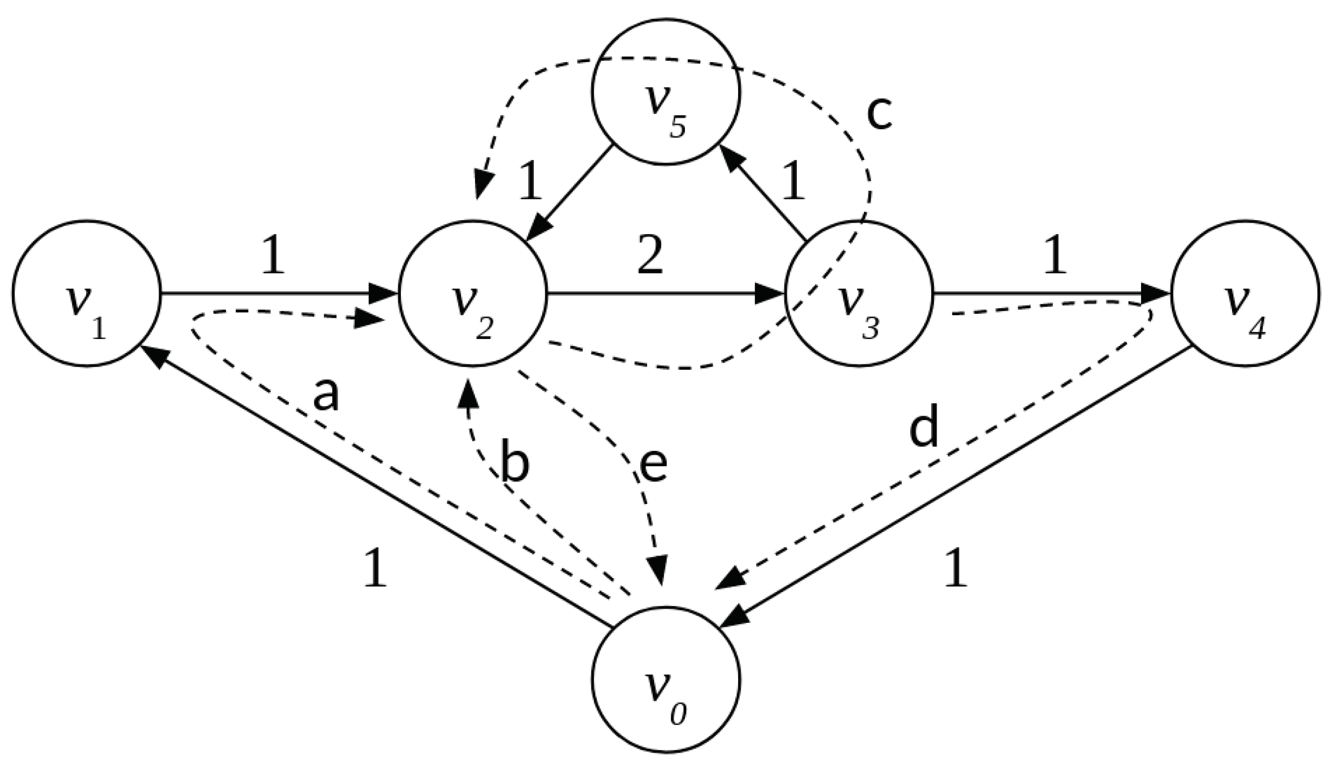
• An obligation network is a directed graph where the nodes6 represent firms and the edges represent the obligations. Parallel edges are allowed to represent multiple obligations between two firms:
• A nominal liability matrix is a matrix representing total obligations or liabilities between firms. We will define special vectors to describe properties of the nominal liability matrix.
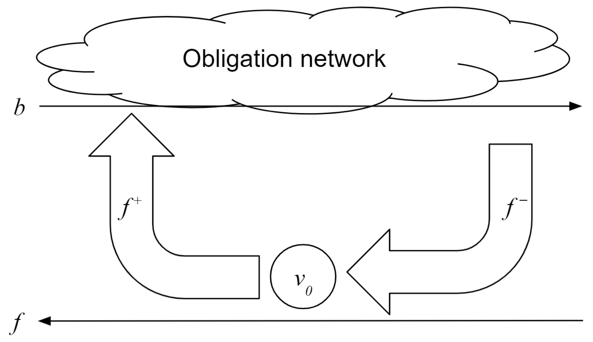
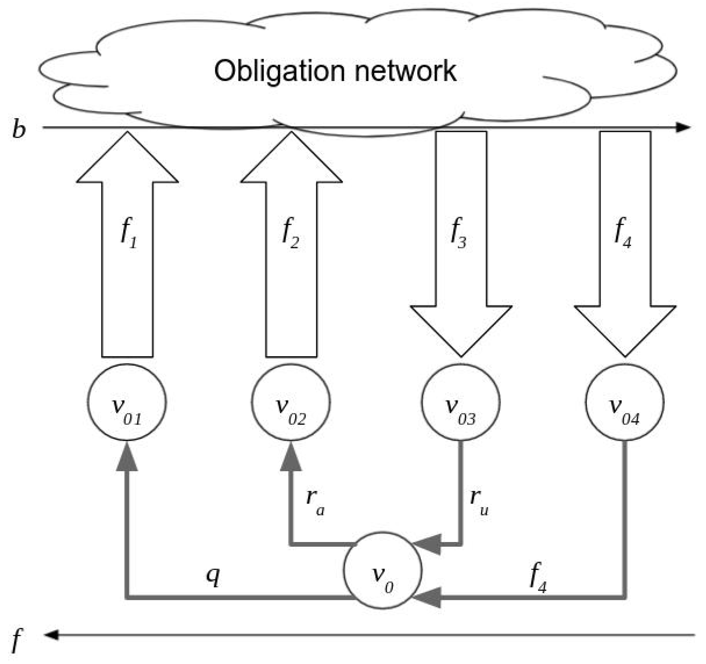
• A payment system is constructed by adding special-function nodes to the obligation network. These special nodes represent sources of funds and a store of value. They can have connections to all nodes in the obligation network, and the set of all connections for each special node is expressed as a vector.

The notation and basic definitions are based on Eisenberg and Noe (2001). We use boldface to denote vector character and uppercase Latin letters for matrices and for sets. $\mathcal{G}$ is reserved for a graph, and $\mathcal{N}=\{1,2,\dots ,n\}\subset \mathbb{N}$ where n represents the number of nodes in the graph. When we extend or generalize the concepts, we use an asterisk superscript.

For any two vectors $\mathbf{x},\mathbf{y}\in {\mathbb{R}}^n$, we define the lattice operations

$$\begin{array}{c}\hfill \begin{array}{cc}\hfill {\mathbf{x}}^{+}& :=(max[x_1,0],max[x_2,0],\cdots ,max[x_n,0])\hfill \\ \hfill {\mathbf{x}}^{-}& :={(-x)}^{+}=(max[-x_1,0],max[-x_2,0],\cdots ,max[-x_n,0])\hfill \\ \hfill \mathbf{x}\wedge \mathbf{y}& :=(min[x_1,y_1],min[x_2,y_2],\cdots ,min[x_n,y_n])\hfill \\ \hfill \mathbf{x}\le \mathbf{y}& \iff x_i\le y_i\forall i\in \mathcal{N}.\hfill \end{array}\end{array}$$

(1)

The vector $\mathbf{0}$ represents an n-dimensional vector all of whose components equal 0, i.e., $\mathbf{0}=(0,\cdots ,0)$. The special brackets $∥·∥$ denote the $l^1$-norm on n. That is,

$$\begin{array}{c}\hfill ∥\mathbf{x}∥:=\sum _{i=1}^n\left|x_i\right|.\end{array}$$

(2)

2.1.1. Obligation Network

Let the directed graph $\mathcal{G}$ represent an obligation network composed of a set $V=\{v_1,\cdots ,v_n\}$ of n vertices (or nodes) representing firms, a set $E=\{e_1,\cdots ,e_m\}$ of m directed edges representing obligations between firms, and the function $o\left(e\right)$ representing the value of a single obligation $e\in E$ between firm $v_i$ and firm $v_j$ (e.g., from a single invoice). The graph $\mathcal{G}$ may contain multiple edges from node $v_i$ to $v_j$, i.e., it can be a ‘multigraph’. We use $(v_i,v_j)\subset E$ to denote the subset of E that corresponds to all the edges between node $v_i$ and node $v_j$. We will use ‘weight’ informally to refer to the value of the obligation associated with a given edge but also to the sum of the values of all the edges linking two nodes $(v_i,v_j)$. In Section 3.1, however, the weight of the network will also be defined formally to denote the sum of all the obligations over the whole network. The meaning in each case should be clear from the context.

These definitions are summarized formally as follows:

$$\begin{array}{cccc}\hfill \mathcal{G}& =(V,E,o)\hfill & \hfill & \mathrm{directed} \left(\mathrm{multi}\right)\mathrm{graph} \mathrm{of} \mathrm{obligations} \mathrm{between} \mathrm{firms}\hfill \end{array}$$

(3)

$$\begin{array}{cccc}\hfill V& =\{v_1,\cdots ,v_n\}\hfill & \hfill & \mathrm{set} \mathrm{of} n \mathrm{nodes} \mathrm{representing} \mathrm{firms}\hfill \end{array}$$

(4)

$$\begin{array}{cccc}\hfill E& =\{e_1,\cdots ,e_m\}\hfill & \hfill & \mathrm{set} \mathrm{of} m \mathrm{edges} \mathrm{representing} \mathrm{individual} \mathrm{obligations}\hfill \end{array}$$

(5)

$$\begin{array}{cccc}\hfill e& \in E\hfill & \hfill & \mathrm{individual} \mathrm{edge} \mathrm{from} \mathrm{set} E\hfill \end{array}$$

(6)

$$\begin{array}{cccc}\hfill o& :E\to \mathbb{R}\hfill & \hfill & \mathrm{assigns} \mathrm{the} \mathrm{value} \mathrm{of} \mathrm{an} \mathrm{obligation} \mathrm{to} \mathrm{each} \mathrm{edge}e\in E.\hfill \end{array}$$

(7)

To develop extended systems and generalizations, we add special nodes such as, following Simić and Milanović (1992), a source and a target node:

$$\begin{array}{cc}\hfill V^{*}& =V\cup \{v_s,v_t\}\hfill \\ \hfill v_s& =\mathrm{the} \mathrm{source} \mathrm{node}\hfill \\ \hfill v_t& =\mathrm{the} \mathrm{target} \mathrm{node}\hfill \end{array}$$

(8)

$$\begin{array}{cc}\hfill E^{*}& =E\cup \{(v_s,v_i):v_i\in V\}\cup \{(v_i,v_t):v_i\in V\},\hfill \end{array}$$

(9)

and in this case there is a single edge between $v_s$, $v_t$ and the vertices in V. The asterisk superscript denotes an extended set, vector, matrix or graph. For example, in this case, ${\mathcal{N}}^{*}=\{1,2,\dots ,n,n+1,n+2\}$.

2.1.2. Nominal Liability Matrix

The nominal liability matrix L is a square $(n\times n)$ matrix each of whose entries is the sum of the obligations between two firms. Since companies do not invoice themselves, L has zeros on the diagonal. Each entry is given by

$$\begin{array}{c}\hfill L_{ij}=\sum _{e\in (v_i,v_j)}o\left(e\right).\end{array}$$

(10)

We will see later that the liability matrix is the basis for the formal definition of a payment system.

The sum of column i of the nominal liability matrix represents the total credit of firm i, and the sum of row i represents the total debt of firm i:

$$\begin{array}{c}\hfill c_i=\sum _{k=1}^n{L}_{ki},d_i=\sum _{k=1}^n{L}_{ik},\end{array}$$

(11)

Equation (11) provides the components of the system-wide credit vector $\mathbf{c}$ and debt vector $\mathbf{d}$. The difference between the credit and debt for each firm gives the obligation network’s net position vector $\mathbf{b}$:7

$$\begin{array}{c}\hfill \begin{array}{cc}\hfill \mathbf{b}& =\mathbf{c}-\mathbf{d}\hfill \\ \hfill b_i& =c_i-d_i,d_i,c_i,b_i\in \mathbb{R},i\in \mathcal{N}.\hfill \end{array}\end{array}$$

(12)

2.1.3. Balanced Net Position Vector

Definition 1.

A vector $\mathbf{b}$ is called balanced if the sum of its components equals 0:

$$\begin{array}{c}\hfill \sum _{i=1}^n{b}_i=0.\end{array}$$

(13)

Theorem 1.

Vector $\mathbf{b}$ representing the net positions of all firms is balanced.

Proof. 

Every obligation that forms the liability matrix contributes towards the net position exactly twice, once as a credit and once as a debt. The sum of all credits is therefore equal to the sum of all debts and the sum of all the net positions equals zero:

$$\begin{array}{c}\hfill \begin{array}{cc}\hfill \sum _{i=1}^n{c}_i& =\sum _{i=1}^n\sum _{k=1}^n{L}_{ki}=\sum _{i=1}^n\sum _{k=1}^n{L}_{ik}=\sum _{i=1}^n{d}_i\hfill \\ \hfill \sum _{i=1}^n{b}_i& =\sum _{i=1}^n(c_i-d_i)=\sum _{i=1}^n{c}_i-\sum _{i=1}^n{d}_i=0.\hfill \end{array}\end{array}$$

(14)

□

Corollary 1.

As a consequence of vector $\mathbf{b}$ being balanced, the sum of its positive vector components must be equal to the sum of the absolute value of its negative vector components:

$$\begin{array}{c}\hfill ∥{\mathbf{b}}^{+}∥=∥{\mathbf{b}}^{-}∥,\end{array}$$

(15)

where ${\mathbf{b}}^{+}$ and ${\mathbf{b}}^{-}$ are calculated as defined in Equation (1).

A balanced net positions vector is important for the analysis of cashflow8 from external sources to the obligation network and vice versa. To visualize these definitions, we use a small obligation network, as shown in Figure 1, that consists of four nodes representing firms and arrows representing the individual obligations between them. The arrow labels represent the values of the obligations.

Equation (16) shows the corresponding nominal liability matrix L. Note that $L_{14}$ is the sum of the two obligations from Firm 1 to Firm 4. Equation (16) also shows the total credit and the total debt for each firm, as defined above.

$$L=\begin{array}{cc}\left[\begin{array}{cccc}0& 1& 0& 3\\ 0& 0& 2& 0\\ 3& 0& 0& 0\\ 0& 0& 1& 0\end{array}\right]& \begin{array}{cc}4& d_1\\ 2& d_2\\ 3& d_3\\ 1& d_4\end{array}\\ \begin{array}{cccc}3& 1& 3& 3\\ c_1& c_2& c_3& c_4\end{array}& \end{array}$$

(16)

Vector $\mathbf{b}$ for this obligation network is calculated as

$$\begin{array}{c}\hfill \begin{array}{cc}\hfill \mathbf{b}=\mathbf{c}-\mathbf{d}=(3,1,3,3)-(4,2,3,1)& =(-1,-1,0,2)\hfill \\ \hfill {\mathbf{b}}^{+}& =(0,0,0,2)\Rightarrow ∥{\mathbf{b}}^{+}∥=2\hfill \\ \hfill {\mathbf{b}}^{-}& =(1,1,0,0)\Rightarrow ∥{\mathbf{b}}^{-}∥=2\hfill \\ \hfill \sum _{i=1}^n{b}_i=∥{\mathbf{b}}^{+}∥-∥{\mathbf{b}}^{-}∥& =0.\hfill \end{array}\end{array}$$

(17)

2.2. Obligation-Clearing with a Liquidity Source

Even if it is not usually possible to clear all the obligations in the network, to make the mathematical treatment more easily understandable, in this section we focus on the case where all the obligations can be cleared. To achieve this, as shown in Figure 2 and unlike the formulation of Simić and Milanović (1992), we introduce a special node $v_0$ in place of $v_s$ and $v_t$ that can act as a liquidity source for all the cashflow towards the obligation network as well as a liquidity sink for all the cashflow from the obligation network. The definitions (8) and (9) for $V^{*}$ and $E^{*}$ are therefore updated as follows:

$$\begin{array}{cc}\hfill V^{*}& =V\cup \left\{v_0\right\}\hfill \end{array}$$

(18)

$$\begin{array}{cc}\hfill E^{*}& =E\cup \{(v_0,v_i):v_i\in V\}\cup \{(v_i,v_0):v_i\in V\}.\hfill \end{array}$$

(19)

The collapse of $v_s$ and $v_t$ into a single node makes it possible to treat a payment system as a new, bigger obligation network to which the same Tetris algorithm can be applied to obtain an optimal use of liquidity. Without such an identification, one would need an additional edge between $v_s$ and $v_t$ with infinite capacity. The implications of this change are discussed in greater detail in Section 3.1.3.

In practice, $v_0$ can be a banking system where every firm in the network has a bank account. It can also be a complementary currency system or any other system with a store of value function. The cashflow is represented by an external cashflow vector $\mathbf{f}\in {\mathbb{R}}^n$. When $f_i>0$, the cashflow for firm i is towards the obligation network, while when $f_i<0$, its cashflow is from the network back to its bank account. By adding the cashflow vector, we have created the payment system $(L,\mathbf{f})$.

Definition 2.

A payment system, denoted $(L,\mathbf{f})$, is an ordered pair composed of an $(n\times n)$ liability matrix L and an $(n\times 1)$ cashflow vector $\mathbf{f}$.

The cashflow available to firms from $v_0$ changes their net positions. If vector $\mathbf{b}$ represents the net positions of firms in the obligation network, let ${\mathbf{b}}_{\ell }$ represent the vector of firms’ net positions in the payment system, where the subscript ℓ is a mnemonic for ‘liquidity’. The value of ${\mathbf{b}}_{\ell }$ is

$$\begin{array}{c}\hfill {\mathbf{b}}_{\ell }=\mathbf{b}+\mathbf{f}.\end{array}$$

(20)

This equation simply states that the net position of every firm is increased by liquidity coming into the obligation network or decreased by liquidity going out of the obligation network. If our goal is to clear all the debt in the network, then—assuming enough liquidity is available—after our intervention the net position of every firm in the payment system has to be zero. In such a scenario, the incoming cashflow is used to pay off the debts of all the firms with negative net positions, whereas the outgoing cashflow carries the liquidity into the bank accounts of the firms with positive (credit) net positions. Therefore,

$$\begin{array}{c}\hfill {\mathbf{b}}_{\ell }=\mathbf{b}+\mathbf{f}=\mathbf{0}\Rightarrow \mathbf{f}=-\mathbf{b}.\end{array}$$

(21)

Given an obligation network and the net positions $\mathbf{b}$ of its members, we now define:

Definition 3.

The Net Internal Debt ($NID$) of the obligation network is the amount of liquidity needed by firms to discharge all the obligations in the network:

$$\begin{array}{c}\hfill NID=\left|\left|{\mathbf{b}}^{-}\right|\right|.\end{array}$$

(22)

The payment system in Figure 2 relates to a real-life situation if we take that $v_0$ is a bank, complementary currency, or some other financial institution that can provide an account-holding function and/or that can serve as a source of liquidity. Thus, the positive values of the cashflow vector ${\mathbf{f}}^{+}={(-\mathbf{b})}^{+}$ represent the payments from individual firms’ accounts at the financial institution, while the negative values of the cashflow vector (or the values of ${\mathbf{f}}^{-}$) represent the payments out of the network and into individual firms’ accounts. Under the current assumption of complete clearance, since the vector $\mathbf{b}$ of the firms’ net positions is balanced, the cashflow vector $\mathbf{f}$ also needs to be balanced. Thus, the total cashflow flowing into the network equals the cashflow out of the network:

$$\begin{array}{c}\hfill \left|\left|{\mathbf{f}}^{+}\right|\right|=\left|\left|{\mathbf{f}}^{-}\right|\right|.\end{array}$$

(23)

Definition 4.

A payment system that can discharge all obligations in an obligation network is balanced.

Theorem 2.

Payment system $(L,\mathbf{f})$ is balanced when $\mathbf{f}=-\mathbf{b}$.

Proof. 

A balanced payment system has to discharge all obligations in the obligation network. That is, for every firm or node in the obligation network, the sum of all incoming and outgoing cashflows has to be 0. Using Equations (11), (12) and (21),

$$\begin{array}{c}\hfill c_i-d_i+f_i=b_i+f_i=b_i-b_i=0\forall i\in \mathcal{N}.\end{array}$$

(24)

□

Corollary 2.

Every balanced payment system satisfies the flow conservation constraint.

Proof. 

The flow conservation constraint requires all flows into a node to be equal to all outflows from a node. For a balanced payment system, this is true for all nodes in the obligation network, as proven in Theorem 2. It is also true for the special node $v_0$ since the sum of all outgoing cashflows $∥{\mathbf{f}}^{+}∥$ equals the sum of all incoming cashflows $∥{\mathbf{f}}^{-}∥$, as shown by Equation (23). □

2.3. Simple Examples

The following examples appear also in Fleischman et al. (2020), but here they are discussed in greater mathematical detail.

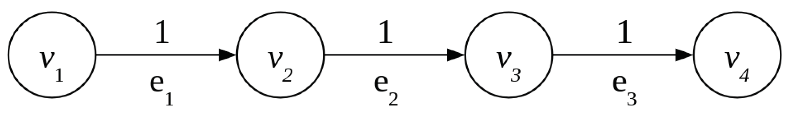
2.3.1. Obligation Chain

To demonstrate the idea of a balanced cashflow vector that clears all obligations in an obligation network, let us observe a small network with four firms that contains only one chain, Figure 3. Firm 1 represented by $v_1$ has an obligation to pay 1 to company $v_2$, and so forth. The three obligations imply the presence of three edges: $\{e_1,e_2,e_3\}$.

It is easy to see from the graph of the obligation network that, if Firm 1 has access to one unit of account of liquid assets, all the firms in the chain can clear all their obligations, resulting in Firm 4 having one unit of account more in their assets. Vector $\mathbf{b}$ for this obligation network is

$$\begin{array}{c}\hfill \begin{array}{cc}\hfill \mathbf{b}& =(-1,0,0,1)\hfill \\ \hfill {\mathbf{b}}^{-}& =(1,0,0,0)\hfill \\ \hfill NID& =\left|\left|{\mathbf{b}}^{-}\right|\right|=1.\hfill \end{array}\end{array}$$

(25)

Therefore, the $NID$—or the amount of external liquidity needed to clear all obligations in this small obligation network containing only one chain—is 1.

As shown in Figure 4, to create a payment system we have to add a new node $v_0$ representing the liquidity source with two edges: $e_5=(v_0,v_1)$ with value $o\left(e_5\right)=1$ that represents the flow of cash into the obligation network, and $e_4=(v_4,v_0)$ with value $o\left(e_4\right)=1$ that represents the flow of cash out of the obligation network. Therefore, clearing the obligation network leaves Firm 1 with 1 unit of account less in their bank account and Firm 4 with 1 unit of account more.

Figure 4 also shows that providing liquidity is not just a problem concerning the total amount of liquid assets available, or $NID$, but also their distribution. As shown in Equation (25), vector ${\mathbf{b}}^{-}$ contains the distribution of liquid assets needed to discharge all obligations in the obligation network. If we let the firms with just enough liquid assets to discharge all obligations act as independent actors, it will take three steps or three individual payments to discharge all obligations in the chain. Using a centralized queue with an LSM, on the other hand, will discharge all obligations simultaneously. This is an example of the time-saving property of LSMs.

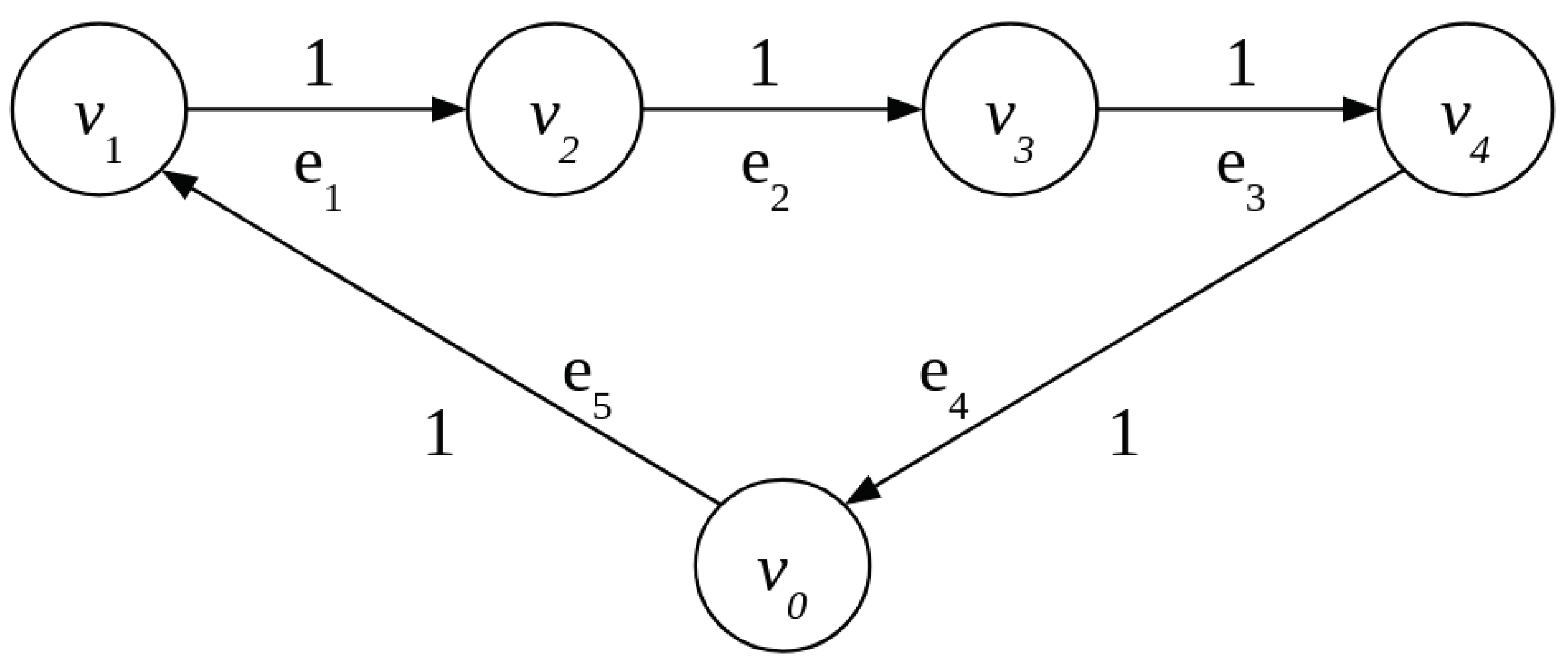
2.3.2. Obligation Cycle

Another interesting example of a small obligation network is a cycle, see Figure 5. Note that, although the edges of a cycle as a topological object could have different weights, in this paper, when we refer to a cycle, we imply that the weights are all equal.

The $NID$ for this network is 0. Therefore, all obligations in the cycle can be cleared without the use of external liquidity. In this special case where the vector $\mathbf{b}=\mathbf{0}$, we can say that the network is balanced. This also means that a cycle meets the flow conservation constraint at all nodes. In other words, for each firm i,

$$\begin{array}{c}\hfill \sum _{k=1}^n{L}_{ki}-\sum _{k=1}^n{L}_{ik}=0\forall i\in \mathcal{N}.\end{array}$$

(26)

This flow conservation constraint equation can be written as a special case of the net positions calculation, Equation (12). Thus, the flow conservation constraint is met when all credits equal all debts for every firm in the cycle.

Although there is no need for external liquidity sources, such a simple cycle cannot be discharged if firms act as independent agents. Without the knowledge of the existence of such a cycle, the payments to discharge the obligations cannot be executed. To discharge all the obligations in a cycle without knowledge of its existence, at least one of the firms in the cycle has to use external liquidity to execute the first payment that then cascades around the cycle. Only with a centralized queue and an LSM can we discharge all obligations in a cycle without the use of external liquidity sources. This is the liquidity-saving property of LSMs.

Cycles in obligation networks are the key to liquidity-saving. At this point, it is worth noting that a cashflow that discharges obligations in the payment system is always a cycle. This cycle can form inside the obligation network as our example in Figure 5, or it can pass through the special node $v_0$ as shown in Figure 4. The flow conservation constraint is met in this case too.

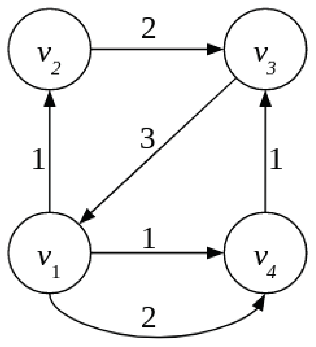
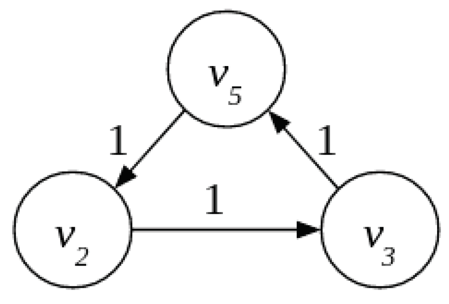
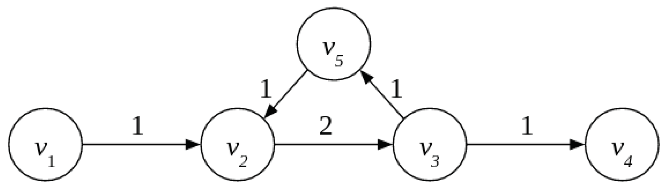
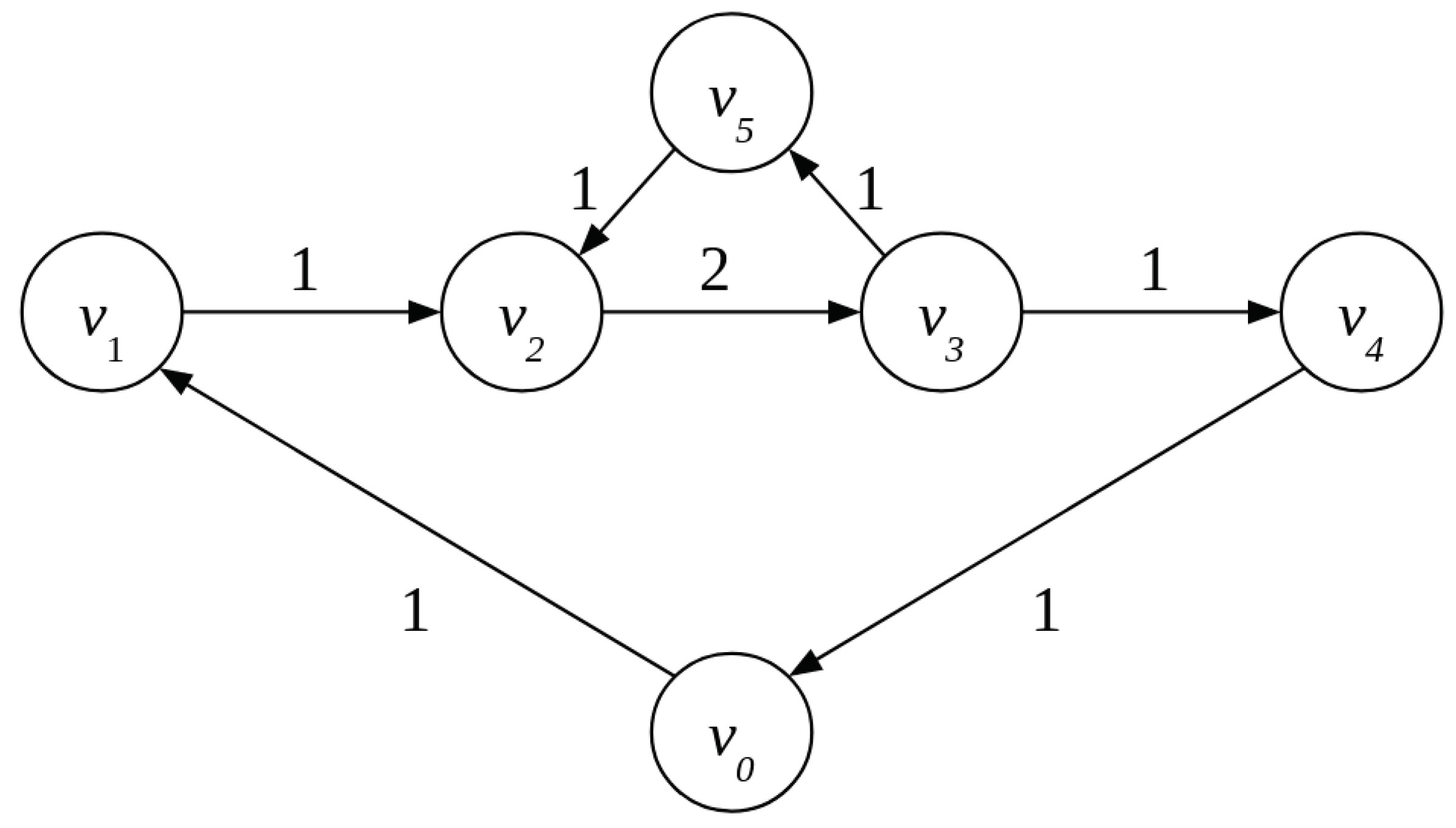
2.3.3. Small Obligation Network with a Chain and a Cycle

Combining a chain and a cycle in a small obligation network, we move closer to a real-life situation. Figure 6 shows the union of the chain and cycle discussed above. The obligation network shown is obviously not balanced and needs external sources of liquidity to discharge all the obligations. The solution is similar to the chain example. The vector $\mathbf{b}$ for this obligation network is

$$\begin{array}{c}\hfill \begin{array}{cc}\hfill \mathbf{b}& =(-1,0,0,1,0)\hfill \\ \hfill \sum _{i=1}^n{b}_i& =0\Rightarrow \mathbf{b} \mathrm{is} \mathrm{balanced}\hfill \\ \hfill ∥\mathbf{b}∥& =2\Rightarrow \mathrm{obligation} \mathrm{network} \mathrm{is} \mathrm{not} \mathrm{balanced}\hfill \\ \hfill ∥{\mathbf{b}}^{-}∥& =1\Rightarrow NID=1.\hfill \end{array}\end{array}$$

(27)

While vector $\mathbf{b}$ is always balanced by definition, the obligation network usually is not. In our case $NID=1$, so this obligation network needs an external liquidity source that can provide 1 unit of account to discharge all the obligations.

The payment system containing chain and cycle is shown in Figure 7. Although there is enough liquidity in such a system to discharge all obligations, it cannot be done if members of the system act as independent agents. The cycle in the system prevents the smooth flow of cash. Firm 2 cannot discharge its obligations even when it receives payment from Firm 1. This creates a gridlock that can be resolved in several ways. One way is for Firm 2 to borrow from an external source, which implies the need for another edge from node $v_0$ to node 2 with value 1. The borrowed funds can be returned to $v_0$ as soon as the payment from Firm 5 to Firm 2 is executed.

This scenario is depicted in Figure 8. Another way to resolve the gridlock is for any other firm in the cycle to borrow from an external source, which would require new edges from node $v_0$. The third option, which still assumes that 1 unit arrives at $v_2$ from $v_1$, is that Firms 2 and 3 agree on the partial discharge of the obligation between them. In this case, the partial payment of 1 unit of account from Firm 2 enables Firm 3 to discharge one of its obligations. If Firm 3 decides to discharge the obligation to Firm 5, the cycle will be discharged in full. This removes the gridlock situation created by the cycle. The flow of 1 unit from $v_0$ through the obligation network is therefore unobstructed and all the remaining obligations can be cleared. If, instead, Firm 3 decides to discharge the obligation towards Firm 4 before Firm 5, we are back to gridlock.

Only putting the whole obligation network in a queue with an LSM will resolve the gridlock without the need for additional liquidity or special agreements among the firms. The solution is to identify the cycles that discharge the obligations simultaneously. This example contains two cycles. The first, smaller cycle involving firms $(2,3,5,2)$ is located inside the obligation network. Obligations with value of 1 can be discharged and the cycle can be removed from the obligation network without affecting the value of vector $\mathbf{b}$. Therefore, the $NID$ or the minimal requirement for external liquidity to discharge all the obligations in the obligation network remains the same. The situation in the payment system after removal of this cycle is a chain with the liquidity source, as shown in Figure 4. This chain with a liquidity source forms the second cycle that is discharged in full with the use of liquidity from the external source.

3. Results

3.1. General Formulation

In this and the following sections, we build on the basic definitions and examples of the previous sections to develop some deeper results with important applications to large-scale payment systems.

3.1.1. A Cycle as a Balanced Payment Subsystem

Although we have made a distinction between an obligation network and a payment system, where the latter includes also a liquidity source, in the general formulation it is more convenient to use the payment system concept in all cases. In particular, an obligation network $\mathcal{G}$ with liability matrix L is a payment system with zero liquidity, i.e., $(L,\mathbf{0})$.

Definition 5.

A payment subsystem $(L^{\prime },{\mathbf{f}}^{\prime })$ of a payment system $(L,\mathbf{f})$ is a payment system obtained by picking a subset ${\mathcal{G}}^{\prime }$ of an obligation network $\mathcal{G}$, and may or may not include also the same liquidity source $v_0$ with a subset of the liquidity available.

Definition 6.

A topological cycle $E_c=\{e_{c1},e_{c2},\cdots e_{ck}\}$ in $\mathcal{G}$ is a closed sequence of k edges that connect nodes $V_c=\{v_{c1},v_{c2}\cdots v_{ck},v_{c1}\}$ consecutively, where $v_{c1}\cdots v_{ck}$ are distinct.

Definition 7.

An obligation network cycle ${\mathcal{G}}_c$ is an ordered triplet $(V_c,E_c,p)$ where all the weights of the edges are set to the minimum obligation in the cycle, i.e., to $p=min\left(o\left(e\right)\right|e\in E_c)$.

Theorem 3.

An obligation network cycle is a balanced payment subsystem.

Proof. 

The net position $b_i$ of every node in such a system is equal to zero since all obligations are equal to p and every node has exactly one incoming and one outgoing edge with the same value:

$$\begin{array}{c}\hfill b_i=p-p=0\forall i\in \{1\cdots k\}.\end{array}$$

(28)

□

Therefore, such a balanced payment subsystem meets the flow conservation constraint (28) and thus does not need external sources of liquidity to clear all its obligations. We note that henceforth the term ‘cycle’ by itself will mean ‘obligation network cycle’.

Theorem 4.

Subtracting a cycle from the obligation network does not change the vector of net positions $\mathbf{b}$.

Proof. 

All the flows in a cycle are equal to p. Therefore, when a cycle is subtracted from the obligation network both credit and debt positions of every firm included in the cycle decrease by the same amount p, leaving the net position vector $\mathbf{b}$ unchanged:

$$\begin{array}{c}\hfill b_i=(c_i-p)-(d_i-p)=c_i-d_i=b_i\forall v_i\in V_c.\end{array}$$

(29)

□

It is important to note that, while from the system’s viewpoint the removal of a balanced payment subsystem does not change, the amount of external liquidity needed to clear all the obligations (i.e., the $NID$, Equation (22), remains the same), from the individual firm’s perspective it makes a big difference, since, with the removal of a balanced payment subsystem, the corresponding gridlock situation is cleared without having to resort to external financing to resolve it. This reduction of the need for external financing can be seen as a reduction of the volume of obligations in the payment system.

3.1.2. Finding the Maximum-Weight Set of Cycles

The problem of cycle elimination from directed graphs to get an acyclic graph is a well-studied area in graph theory. An overview of graph cycles is provided by Kavitha et al. (2009), and a fast parallel algorithm for finding the cycles in a graph is proposed in Cui et al. (2017). Here, we develop our own method, starting with the concept of “weight”.

Definition 8.

We define the weight of an obligation network with set of edges E as a function $w:\mathcal{G}\to \mathbb{R}$ whose value is the sum of all the obligations in the network:

$$\begin{array}{c}\hfill w\left(\mathcal{G}\right)=\sum _{e\in E}o\left(e\right).\end{array}$$

(30)

Similarly, a cycle ${\mathcal{G}}_c$ of length k with all its obligations of value p has weight:

$$\begin{array}{c}\hfill w\left({\mathcal{G}}_c\right)=pk.\end{array}$$

(31)

Removing a cycle ${\mathcal{G}}_c$ from the obligation network reduces its weight. The weight of the residual obligation network ${\mathcal{G}}_r$ is:

$$\begin{array}{c}\hfill w\left({\mathcal{G}}_r\right)=w\left(\mathcal{G}\right)-w\left({\mathcal{G}}_c\right)\end{array}$$

(32)

Therefore, reducing the debt of the individual firms can be achieved by removing all the cycles from the obligation network, which is also equivalent to resolving all the gridlocks. To achieve this, we need to solve the following problem:

Problem 1.

Find a sequence of cycles ${\mathcal{G}}_{ci}$ and residual obligation networks ${\mathcal{G}}_{ri}$ such that

$$\begin{array}{c}\hfill \sum _{i=1}^{q}w\left({\mathcal{G}}_{ci}\right)\mathit{is}\mathit{maximum},\end{array}$$

(33)

where

$$\begin{array}{c}\hfill \begin{array}{cc}\hfill {\mathcal{G}}_{c1},{\mathcal{G}}_{r1}& \subset \mathcal{G}\hfill \\ \hfill {\mathcal{G}}_{c2},{\mathcal{G}}_{r2}& \subset {\mathcal{G}}_{r1}\hfill \\ \hfill & ⋮\hfill \\ \hfill {\mathcal{G}}_{cq},{\mathcal{G}}_{rq}& \subset {\mathcal{G}}_{r(q-1)},\hfill \end{array}\end{array}$$

(34)

${\mathcal{G}}_{c1},\cdots ,{\mathcal{G}}_{cq}$ are cycles, and q is the number of cycles present in the network.

Sequential elimination of cycles from the obligation network will always lead to a residual network ${\mathcal{G}}_{rq}$ that is acyclic. The exact number of cycles q that will be eliminated is not known upfront and depends on the methods used to find them. For example, every directed acyclic graph has a topological ordering, i.e., an ordering of the vertices such that the start-point of each directed edge occurs earlier in the ordering than the end-point of that edge. The ordering can be found in linear time using Kahn’s algorithm for topological sorting (Kahn 1962). This would be a possible formal test. Alternatively, the cycle-finding algorithm usually has a “cycle not found” exit condition, which is also an acyclic graph test: the algorithm repeats until a cycle can be found and, when no cycles can be found any longer, whatever is left is acyclic.

Definition 9.

Given an obligation network $\mathcal{G}$, a maximum-weight set of cycles $\{{\mathcal{G}}_{c1},\cdots ,{\mathcal{G}}_{cq}\}$ is one of the solutions to Problem 1.9

It is known that there is always a way to eliminate all the cycles and that the solution is not unique. The problem is that the removal of one cycle can break other embedded cycles,10 so the solution depends on the order in which the cycles are found. This makes finding the maximum-weight set of cycles even harder. The solution is not to look for cycles at all but to use the concept of balanced payment system and minimum-cost flow instead.

3.1.3. The Minimum-Cost Flow Problem

In the context of the present paper, the minimum-cost flow (MCF) problem (Király and Kovács 2012) presents a terminology challenge because both ‘cost’ and ‘flow’ are overloaded. The ‘cost’ in MCF has nothing to do with the cost of transactions or invoices. Rather, it is a cost of attrition in following different paths through a continuous system or a discrete network. In addition, the ‘flow’ has nothing to do with the cashflows we have been discussing; rather, it refers to movement through the same system or network. Thus, we seek to pose the problem of optimal liquidity-saving as one where the ‘MCF flow’ is a flow through the network that avoids all the cycles. It is all about avoiding the additional costs associated with flows that go through cycles, since that tends to lengthen the paths and therefore to make them too “expensive”. In this formulation, the ‘MCF cost’ is uniform and set to 1 for all network hops, for the sake of simplicity.

The starting point in applying the MCF method to the optimization of the obligation-clearing problem is a perfectly balanced payment system as described in Section 2.2. We have an obligation network $\mathcal{G}$ with associated nominal liability matrix L, net position vector $\mathbf{b}$, and external cashflow vector $\mathbf{f}=-\mathbf{b}$, forming a balanced payment system $(L,\mathbf{f})$. We know that the external-liquidity cashflow through this balanced payment system equals the $NID$ as defined in Equation (22). Now, we try to find a balanced payment system $(M,\mathbf{f})$, where the nominal MCF liability matrix M represents the minimum-weight sub-network ${\mathcal{G}}_m$ of the obligation network $\mathcal{G}$ subject to a specific constraint. Namely, we are looking for a matrix M the sum of whose elements is a function11 that we wish to minimize subject to the constraint that its column sum (or credit vector) minus its row sum (or debt vector) equals matrix L’s net positions vector $\mathbf{b}$.

To find such nominal liability matrix M, we have to:

• Define the object function as a Grandsum function $\mu :{\mathbb{R}}^{n^2}\to \mathbb{R}$, which is the sum of all the elements of a given square $n\times n$ matrix. Looking for the minimum of the function $\mu \left(M\right)$ is equivalent to looking for the minimum-weight sub-network ${\mathcal{G}}_m$.
• Make sure that the payment system $(M,\mathbf{f})$ is balanced. The constraint above ensures this since $(L,\mathbf{f})$ is balanced by construction. In fact, since $\mathbf{f}=-\mathbf{b}$ and M uses the same cashflow vector $\mathbf{f}$, ensuring that M has the same net position vector $\mathbf{b}$ is enough to guarantee that $(M,\mathbf{f})$ will be balanced too.
• Make sure we are not introducing edges between nodes in sub-network ${\mathcal{G}}_m$ that do not exist in the obligation network $\mathcal{G}$. Therefore, all matrix elements $M_{ij}$ must have a value between 0 and $L_{ij}$.

The optimization problem is therefore posed formally as follows:

Problem 2.

Find the liability matrix M of the obligation network ${\mathcal{G}}_m$ such that its Grandsum function μ is minimum:

$$\begin{array}{c}\hfill min\mu \left(M\right)=min\sum _{i=1}^n\sum _{j=1}^n{M}_{ij}\end{array}$$

(35)

subject to the constraints:

$$\begin{array}{cccc}\hfill \sum _{k=1}^n{M}_{ki}-\sum _{k=1}^n{M}_{ik}& =b_i\hfill & \hfill & \forall i\in \mathcal{N}\hfill \end{array}$$

(36)

$$\begin{array}{cccc}\hfill 0\le M_{ij}& \le L_{ij}\hfill & \hfill & \forall i,j\in \mathcal{N}.\hfill \end{array}$$

(37)

The reason we need to find M is that it is the solution to the standard MCF problem as defined in graph theory. The solution to the MCF problem equals all flows in a cyclic structure that includes the liquidity source, i.e., from $v_0$, represented by vector ${\mathbf{b}}^{-}$, through the obligation network and back to the liquidity source, represented by vector ${\mathbf{b}}^{+}$. We are looking for the shortest paths that can carry the $NID$ through the obligation network. Because from the MCF point of viewcycles are inefficient, M always represents an acyclic network composed only of chains.

We can map our definition of the optimization problem to the standard MCF problem (Király and Kovács 2012). The difference to the standard MCF problem is that we do not use MCF costs assigned to individual edges of the network. The goal as defined in Equation (35) is the same: finding the minimum flow. In the standard MCF problem definition, the constraint (36) is called a ‘flow conservation constraint’. The constraint conserves the balance of flows through the nodes of the network. The constraint (37) is called capacity constraint in the standard MCF problem. We are setting the limit to the maximum flow between two nodes as the sum of all the individual obligations between those nodes. In the standard MCF solution, the cost of the flows through different edges can vary. In our case, the cost of the flow through different edges is the same, since we do not want to prioritize any specific flow or firm. Thus, using the standard MCF solution all costs of a flow through an edge are set to 1.

Any minimum-cost flow algorithm will find a set of chains that can carry the max-flow $NID$ through the obligations at minimum cost. There are many known algorithms to solve the minimum-cost flow problem, e.g., see Király and Kovács (2012) for an overview. A polynomial-time algorithm was proposed by Orlin (1996). The solution is not unique, but the value and the cost of the flow through the edges of the set of minimum-cost flows are always the same.

Theorem 5.

Subtracting the min cost-max flow solution M from the nominal liability matrix L leaves a balanced payment subsystem $(T,\mathbf{0})$ that requires no external liquidity source to clear the obligations:

$$\begin{array}{c}\hfill T=L-M.\end{array}$$

(38)

Proof. 

We need to prove that all the edges in the remaining nominal liability matrix T are part of a cycle. As such, no liquidity is needed to clear all the obligations in the network T, which implies that it must be balanced. Therefore, the vector $\mathbf{b}$ for the matrix T must be $\mathbf{0}$.

We can show that

$$\begin{array}{c}\hfill \sum _{k=1}^n{T}_{ki}-\sum _{k=1}^n{T}_{ik}=0,\forall i\in \mathcal{N},\end{array}$$

(39)

is always true since L and M have the same vector $\mathbf{b}$. First, (38) trivially implies that

$$\begin{array}{cc}\hfill T_{ij}& =L_{ij}-M_{ij}.\hfill \end{array}$$

(40)

Then, using (11) and (12), we have that, $\forall i\in \mathcal{N}$,

$$\begin{array}{c}\hfill b_i=c_i-d_i=\sum _{k=1}^n{L}_{ki}-\sum _{k=1}^n{L}_{ik}=\sum _{k=1}^n(L_{ki}-L_{ik}).\end{array}$$

(41)

In addition, from the definition of the MCF Problem (36),

$$\begin{array}{c}\hfill b_i=\sum _{k=1}^n{M}_{ki}-\sum _{k=1}^n{M}_{ik}=\sum _{k=1}^n(M_{ki}-M_{ik}).\end{array}$$

(42)

Using (41) and (42) and reordering the sums,

$$\begin{array}{c}\hfill \begin{array}{cc}\hfill b_i-b_i& =0\hfill \\ \hfill \sum _{k=1}^n(L_{ki}-L_{ik})-\sum _{k=1}^n(M_{ki}-M_{ik})& =0\hfill \\ \hfill \sum _{k=1}^n(L_{ki}-M_{ki})-\sum _{k=1}^n(L_{ik}-M_{ik})& =0\hfill \\ \hfill \sum _{k=1}^n{T}_{ki}-\sum _{k=1}^n{T}_{ik}& =0,\hfill \end{array}\end{array}$$

(43)

thereby showing that the vector $\mathbf{b}$ for the matrix T always equals $\mathbf{0}$. This proves that T is composed of cycles only. □

Corollary 3.

T is a maximum-weight balanced payment subsystem.

Proof. 

Since we subtracted the minimum value of chains M from L, the remaining obligation network T consists of the maximum value of cycles. Since we have just proven that T is a balanced payment system, T must be a maximum-weight balanced payment subsystem of L. □

3.2. Using Balanced Payment Subsystems in the Trade Credit Market

In normal business situations, we seldom have enough cash available to clear all our obligations. Therefore, it would be helpful to adjust our model to reflect the scarcity of liquidity.

The trade credit market is an interesting example since there are no liquidity sources at all. We can look at it as a payment system where the external financing vector $\mathbf{f}$ equals $\mathbf{0}$, i.e., $(L,\mathbf{0})$. Still, it is possible to discharge the obligations bilaterally or multilaterally by applying the balanced payment subsystem idea.

Theorem 6.

Subtracting a balanced payment subsystem from the payment system does not change the net position vector $\mathbf{b}$.

Proof. 

We adopt a similar strategy as in the proof of Theorem 4. We have a nominal liability matrix L with a net position vector $\mathbf{b}$, credit vector $\mathbf{c}$ and debt vector $\mathbf{d}$. The balanced payment subsystem $(T,\mathbf{0})$ satisfies the flow conservation constraint, as shown in Corollary 2. Therefore, the cashflow into each node of the balanced payment subsystem equals the outflow. Following Eisenberg and Noe (2001), for the nominal liability matrix T of the balanced payment subsystem $(T,\mathbf{0})$, we can define a ‘clearing vector’ $\mathbf{p}=(p_1,p_2,\cdots ,p_n)$ such that $p_i$ stands for the flow into or out of node i. This is a generalization of the constant p scalar of Theorem 4. Now, we subtract the balanced payment subsystem T, such that

$$\begin{array}{c}\hfill L-T=M,\end{array}$$

(44)

and show that the net position vector of the resulting nominal liability matrix M equals the net position vector of the nominal liability matrix L:

$$\begin{array}{c}\hfill {\left(b_i\right)}_{(L-T)}={\left(b_i\right)}_M=(c_i-p_i)-(d_i-p_i)=c_i-d_i={\left(b_i\right)}_L\forall i\in \mathcal{N}.\end{array}$$

(45)

□

The method to discharge the maximum volume of obligations without using any liquidity can be summarized by the following steps:

• Collect obligations to form an obligation network $\mathcal{G}$.
• Form a nominal liability matrix L and a payment system $(L,\mathbf{0})$ without external financing.
• Find a maximum-weight balanced payment subsystem T.
• Discharge the obligations in the balanced payment subsystem $(T,\mathbf{0})$ by sending set-off notices to all pertinent firms.
• Subtract the balanced payment subsystem T, such that $L-T=M$.
• Leave the remaining obligations in the nominal obligation matrix M to be discharged using the normal bank payment system.

We call matrix T a ‘Tetris solution’. Depending on the economic conditions, in Slovenia, TCT discharges between 1% and 7.5% of GDP per year in saved liquidity towards the clearing of trade credit obligations. This is an example of an LSM in the trade credit market with a significant contribution to national financial stability.

4. Discussion: Practical Trade Credit Formulation

Having presented the basic mathematics in the previous sections, in this section we elaborate the payment system model further for the benefit of practitioners and application developers.

4.1. Formal Model for Single Liquidity Source

From an applied viewpoint, it is helpful to explain the functioning of a general liquidity source in terms of an abstraction whereby different sub-functions are represented by separate nodes. In particular, two main functions are given by the accounting of liquidity balances and the accounting of credit lines. Each function, in turn, requires two nodes, one for cashflow from the source towards the network and the other for the reverse flow, leading to a total of four auxiliary nodes. Each of the four nodes holds as many accounts as there are companies in the network, i.e., $\left|\mathcal{N}\right|=n$. This is an abstraction in the sense that the value of $|{\mathcal{N}}^{*}|$ remains $n+1$; it is not affected by the auxiliary nodes, i.e., it is not $n+5$.

Figure 9 shows the payment system with the auxiliary nodes. This model was used to analyse the potential for integrating TCT with the Sardex complementary currency (Fleischman et al. 2020). It can be adapted to cover a wide variety of use cases, so here we explain a very similar but more general model relevant to a bank. In particular, corresponding to the roles of the four auxiliary nodes, the cashflow vector $\mathbf{f}$ for the case of a single liquidity source $v_0$ can be expressed as a vector sum of the four different “component” vectors shown in the figure:

• ${\mathbf{f}}_1$: cashflows from firms’ bank accounts (only positive balances used)
• ${\mathbf{f}}_2$: overdraft cashflows up to firms’ credit lines
• ${\mathbf{f}}_3$: cashflows to repay firms’ overdrafts (different set of firms from ${\mathbf{f}}_{\mathbf{2}}$’s)
• ${\mathbf{f}}_4$: cashflows into firms’ bank accounts (different set of firms from ${\mathbf{f}}_{\mathbf{1}}$’s),

where the ‘different set of firms’ refers only to the non-zero components of the vectors in question, since $|{\mathbf{f}}_i|=n\forall i$. In other words, although each vector ${\mathbf{f}}_i$ has the same length as all the others, the non-zero components of each are different pairwise for ${\mathbf{f}}_1$ and ${\mathbf{f}}_4$ and for ${\mathbf{f}}_2$ and ${\mathbf{f}}_3$. As shown in the figure, ${\mathbf{f}}_1$ and ${\mathbf{f}}_2$ issue from $v_{01}$ and $v_{02}$, respectively, whereas ${\mathbf{f}}_3$ and ${\mathbf{f}}_4$ lead from the network back towards $v_{03}$ and $v_{04}$, respectively. The resultant vector $\mathbf{f}$, then, is given by

$$\begin{array}{cc}\hfill \mathbf{f}& ={\mathbf{f}}_1+{\mathbf{f}}_2-{\mathbf{f}}_3-{\mathbf{f}}_4.\hfill \end{array}$$

(46)

Each of the component vectors is calculated by means of the following lattice algebra expressions:

$$\begin{array}{cccc}\hfill {\mathbf{f}}_1& ={\mathbf{b}}^{-}\wedge {\mathbf{q}}^{+}\hfill & \hfill & {\mathbf{q}}^{+}\mathrm{holds}\mathrm{the}\mathrm{available}\mathrm{funds}\mathrm{in}\mathrm{firms}’\mathrm{accounts}\hfill \end{array}$$

(47)

$$\begin{array}{cccc}\hfill {\mathbf{f}}_2& ={\mathbf{r}}_a\wedge ({\mathbf{b}}^{-}-{\mathbf{f}}_1)\hfill & \hfill & {\mathbf{r}}_a\mathrm{holds}\mathrm{the}\mathrm{available}\mathrm{credit}\mathrm{lines}\hfill \end{array}$$

(48)

$$\begin{array}{cccc}\hfill {\mathbf{f}}_3& ={\mathbf{b}}^{+}\wedge {\mathbf{r}}_u\hfill & \hfill & {\mathbf{r}}_u\mathrm{tallies}\mathrm{the}\mathrm{overdraft}\left(\mathrm{loan}\right)\mathrm{repayments}\mathrm{due}\hfill \end{array}$$

(49)

$$\begin{array}{cccc}\hfill {\mathbf{f}}_4& ={\mathbf{b}}^{+}\wedge ({\mathbf{b}}^{+}-{\mathbf{f}}_3)\hfill & \hfill & \mathrm{the}\mathrm{remainder}\mathrm{after}\mathrm{repayment}\mathrm{can}\mathrm{be}\mathrm{saved}.\hfill \end{array}$$

(50)

We remark that the meet operation in (50) is redundant, since $({\mathbf{b}}^{+}-{\mathbf{f}}_3)$ by itself would give the same result. However, the extended version is kept to highlight the symmetry with (48). To explain what ‘available credit line’ in (48) means, we need to explain how vector ${\mathbf{r}}_a$ is constructed. To that end, let $x_i$ be the balance of account i. In principle, this value could be positive or negative but because we have already taken positive balances into account with Equation (47), it can only be zero or negative, i.e., $x_i\le 0$. Let $y_i$ be that account’s credit line, which, for the purposes of this explanation, is taken as a negative number such that $y_i\le x_i$. Then, by available credit lines, we mean the funds available; namely, ${\left(r_a\right)}_i=x_i-y_i$, such that ${\left(r_a\right)}_i\ge 0$ necessarily. We emphasize that in this model nothing stops the same firm i from appearing in the calculations of both ${\mathbf{f}}_1$ and ${\mathbf{f}}_2$, which corresponds to a case where $q_i\ge 0$ and $b_i^{-}>q_i$. Finally, although for mutual credit there is no interest, in a more general setting, $r_u$ can be defined as ‘the principal and interest repayment due’ at the time of the multilateral set-off.

Having explained the data structures and the functions used by this model, we now briefly summarize the high-level algorithm in five steps, where the output of each is the input to the next:

• After all the obligations have been uploaded into the repository (which could be a blockchain), an obligation network exists, but the net positions are not yet known. The network is the first output, and the input to Step 2.
• Based on the network, the net positions are calculated, i.e., the components of vector $\mathbf{b}$. This is the output of Step 2 and the input to Step 3.
• The cyclic structure is determined. This is the output of Step 3 and the input to Step 4.
• The cyclic structure is removed from the obligation network, i.e., multilateral set-off is performed. This results in a new, acyclic obligation network with obligation amounts that, usually, are the same as before for a subset of firms, smaller for another subset, and zero for a third subset, which is the complement of the first two.
• The TCT multilateral set-off process is completed when set-off notices are sent to all the firms instructing them about what is left to pay.

The optimization goal of the TCT algorithm is to achieve total clearing, i.e., a balanced payment system. This objective is constrained by the availability of customers’ funds and by the lending policy of fiduciary and lending institutions. The lending policy, in turn, is formulated in terms of the maximum overdraft exposure the lending institution allows itself and of the individual credit lines it affords the firms. The maximum exposure of the overdraft facility $r^{max}\in \mathbb{R}$ is set by the lending institution and represents a constraint on the maximum value that the capacity of the edge connecting $v_0$ with $v_{02}$ can assume. The repayment of loans/overdraft vector ${\mathbf{r}}_u$ represents the current overdraft taken by individual firms, which is the amount that has to be repaid to balance their bank accounts. The actual overdraft facility’s repayment cashflow, however, is set by ${\mathbf{f}}_3$. Node $v_{04}$ accepts the remaining cashflow ${\mathbf{f}}_4$ out of the obligation network back to the “master” accounts-holding node $v_0$. When the distribution of the available external liquidity sources is equal to or exceeds the components of vector ${\mathbf{b}}^{-}$ at all points, a balanced payment system can be formed. This condition is met when:

$$\begin{array}{cc}\hfill {\mathbf{f}}_1+{\mathbf{f}}_2& \ge {\mathbf{b}}^{-}\hfill \end{array}$$

(51)

$$\begin{array}{cc}\hfill ∥{\mathbf{f}}_2∥& \le r^{max}.\hfill \end{array}$$

(52)

If both conditions are satisfied, there are enough external liquidity sources in the firms’ account holdings and overdraft facilities to form an external financing vector $\mathbf{f}$ that satisfies the condition for a balanced payment system $(L,\mathbf{f})$, Equation (21):

$$\begin{array}{c}\hfill \mathbf{f}=-\mathbf{b}.\end{array}$$

If the conditions for a balanced payment system are not met, it makes sense to find a balanced payment subsystem to facilitate the discharge of as many obligations as possible.

4.2. Generalization to Multiple Sources

The case of multiple sources is handled in exactly the same way for each source. To distinguish between the different sources, we simply add a subscript such that, for each source j,

$$\begin{array}{cc}\hfill {\mathbf{f}}_j& ={\mathbf{f}}_{j1}+{\mathbf{f}}_{j2}-{\mathbf{f}}_{j3}-{\mathbf{f}}_{j4},\hfill \end{array}$$

(53)

and

$$\begin{array}{cc}\hfill \mathbf{f}& =\sum _{j=1}^{n_s}{\mathbf{f}}_j,\hfill \end{array}$$

(54)

where $n_s$ is the number of independent liquidity sources and for each source the same Equations (47)–(50) apply for its component vectors in each case.

Figure 10 shows a visualization of the cyclic structure for a case where $n_s=3$ (EUBOF 2021). Each node shown is a firm or an individual. The arcs of the graph denote bilateral obligations (IOUs), not currency flows. The picture does not show all the obligations between these roughly 3000 points, it only shows the obligations that can be cleared with (red, blue, yellow) or without (green) the liquidity sources. To utilize multiple liquidity sources, the exchange rate must be set to an agreed unit of account (e.g., the Euro) for each party at the moment of clearing, which is near-instantaneous. Yellow could represent fiat held in bank accounts, red CBDC balances, and blue cryptocurrencies. A fourth source could be added representing mutual credit.

4.3. Optimizing the Use of Available Liquidity

The setup and algorithm of the previous section can be adjusted unilaterally by individual firms. For example, a firm may wish to use its credit line even though it still has cash available in its bank account. Similarly, a bank may set different global or local constraints. In general, however, the optimal solution for the payment system described above can be obtained by applying the idea from Theorem 5 to the payment system in its entirety. This ensures the maximum total obligation settlement amount with the available liquidity sources. Leaving the execution of payments to the discretion of the individual firms will yield a sub-optimal solution since firms do not have sufficient information about the payment system.

To use the idea of removing the maximum weight of cycles from the payment system, we have to transform the payment system into an extended nominal liability matrix, where liquidity sources become new nodes and the desired cashflows become new obligations. Let us denote such an extended nominal liability matrix by $L^{*}$. Let us apply the MCF algorithm to find an extended minimum-cost flow $M^{*}$ and then the extended maximum weight set of cycles $T^{*}$ by using the equation

$$\begin{array}{c}\hfill L^{*}-M^{*}=T^{*}.\end{array}$$

(55)

Theorem 7.

The extended maximum-weight set of cycles $T^{*}$ discharges the maximum amount of obligations in the obligation network with the available liquidity.

Proof. 

The extended nominal liability matrix has no external liquidity sources, by construction. Therefore, new sources of liquidity are needed to discharge the obligations in $M^{*}$. This is consistent with how we defined the MCF problem in Section 3.1.3. The cycles in $T^{*}$ as shown in Corollary 3, therefore, use the available distribution of liquidity inside $L^{*}$ to discharge the maximum volume of obligations in the obligation network. □

5. Conclusions

The generalization of the payment system presented allows for the implementation of an LSM outside the interbank payment systems. The potential in trade credit markets is proven by 30 years of positive experience with trade credit clearing in Slovenia. New developments in e-invoicing and tax compliance create new opportunities to implement LSMs in the trade credit market in the rest of Europe and beyond.

In Fleischman et al. (2020), we made the empirical claim that the most basic use of the TCT algorithm delivers a significant decrease of the mutual indebtedness present in an obligation network. In this paper, we have provided the mathematical proofs for why a decrease is assured as long as there are cycles in the network, although we did not address mathematically what ‘significant’ might mean. Building on that, its extended use, where the obligation network is transformed into a payment system, allows for an efficient use of external liquidity sources to discharge the maximum amount of debt possible. In this paper, we proved the maximum claim, although again how significant that might be in economic terms remains a context-dependent question that will be explored in future work. From an applied mathematics point of view; therefore, the original contribution of the paper has been the introduction of a liquidity node with a store of value function in obligation-clearing and the demonstration that the case with one or more liquidity sources can be solved with the same mathematical machinery that is used for obligation-clearing without liquidity.

From a wider perspective, obligation-clearing and complementary currencies such as mutual credit can be seen as examples of ‘collaborative finance’. There are new services developing that collect a huge amount of trade credit information that can be utilized to implement the idea of the balanced payment subsystem. For example, new methods of information exchange using decentralized ledger technologies (DLTs) and decentralized finance (DeFi) call for the implementation of LSMs that provide solutions in environments where liquidity is not readily available and that can help communities of small firms in development and humanitarian crisis contexts in significant ways. Further opportunities for implementation are with complementary currencies and crypto assets that can enable the discharging of obligations issued in fiat currency as external sources of liquidity. This way, the impact of the benefits of mutual trust characteristic of complementary currency communities, which are most visible at small scales, could be transmitted to the national economy and the wider society.

References

1. Abraham, David J., Avrim Blum, and Tuomas Sandholm. 2007. Clearing algorithms for barter exchange markets: Enabling nationwide kidney exchanges. Paper present at the 8th ACM Conference on Electronic Commerce, San Diego, CA, USA, June 11–15; pp. 295–304. [Google Scholar]
2. Allen, Franklin, Meijun Qian, and Jing Xie. 2018. Understanding informal financing. Journal of Financial Intermediation 39: 19–33. [Google Scholar] [CrossRef]
3. Bardoscia, Marco, Paolo Barucca, Stefano Battiston, Fabio Caccioli, Giulio Cimini, Diego Garlaschelli, Fabio Saracco, Tiziano Squartini, and Guido Caldarelli. 2021. The physics of financial networks. Nature Reviews Physics 3: 490–507. [Google Scholar] [CrossRef]
4. Bech, Morten, and Kimmo Soramäki. 2001. Gridlock Resolution in Interbank Payment Systems. Research Discussion Papers 9/2001, Bank of Finland. Available online: https://EconPapers.repec.org/RePEc:bof:bofrdp:2001_009 (accessed on 23 June 2021).
5. Börner, Lars, and John William Hatfield. 2017. The Design of Debt-Clearing Markets: Clearinghouse Mechanisms in Preindustrial Europe. Journal of Political Economy 125: 1991–2037. [Google Scholar] [CrossRef] [Green Version]
6. Cui, Huanqing, Jian Niu, Chuanai Zhou, and Minglei Shu. 2017. A Multi-Threading Algorithm to Detect and Remove Cycles in Vertex- and Arc-Weighted Digraph. Algorithms 10: 115. [Google Scholar] [CrossRef] [Green Version]
7. Eisenberg, Larry, and Thomas H. Noe. 2001. Systemic Risk in Financial Systems. Management Science 47: 236–49. Available online: http://www.jstor.org/stable/2661572 (accessed on 23 June 2021). [CrossRef]
8. EUBOF. 2021. Central Bank Digital Currencies and a Euro for the Future. Technical Report, EU Blockchain Observatory and Forum. Available online: https://www.eublockchainforum.eu/sites/default/files/reports/CBDC%20Report%20Final.pdf (accessed on 5 July 2021).
9. Fleischman, Tomaž, Paolo Dini, and Giuseppe Littera. 2020. Liquidity-Saving through Obligation-Clearing and Mutual Credit: An Effective Monetary Innovation for SMEs in Times of Crisis. Journal of Risk and Financial Management 13: 295. Available online: https://www.mdpi.com/1911-8074/13/12/295 (accessed on 23 June 2021). [CrossRef]
10. Foote, Elizabeth. 2014. Information asymmetries and spillover risk in settlement systems. Journal of Banking & Finance 42: 179–90. Available online: http://www.sciencedirect.com/science/article/pii/S0378426614000120 (accessed on 23 June 2021).
11. Gaffeo, Edoardo, Lucio Gobbi, and Massimo Molinari. 2019. The economics of netting in financial networks. Journal of Economic Interaction and Coordination 14: 595–622. [Google Scholar] [CrossRef]
12. Galbiati, Marco, and Kimmo Soramäki. 2010. Liquidity-Saving Mechanisms and Bank Behaviour. Bank of England Working Paper 400. Available online: http://dx.doi.org/10.2139/ssrn.1650632 (accessed on 23 June 2021).
13. Garratt, Rodney, and Peter Zimmerman. 2020. Centralized netting in financial networks. Journal of Banking & Finance 112: 105270. [Google Scholar]
14. Gavrila, Lucian-Ionut, and Alexandru Popa. 2021. A novel algorithm for clearing financial obligations between companies—An application within the romanian ministry of economy. Algorithmic Finance 9: 49–60. [Google Scholar] [CrossRef]
15. Gazda, Vladimír, Denis Horváth, and Marcel Resovsky. 2015. An application of graph theory in the process of mutual debt compensation. Acta Polytechnica Hungarica 12: 7–24. [Google Scholar]
16. Glasserman, Paul, and Peyton Young. 2016. Contagion in Financial Networks. Journal of Economic Literature 54: 779–831. [Google Scholar] [CrossRef] [Green Version]
17. Gobbi, Lucio. 2018. Clearing Mechanism in Real and Financial Markets. Ph.D. thesis, University of Trento, Trento, Italy. Available online: http://eprints-phd.biblio.unitn.it/3097/1/tesi_Lucio_Gobbi.pdf (accessed on 14 August 2021).
18. Hüser, Anne-Caroline. 2015. Too Interconnected to Fail: A Survey of the Interbank Networks Literature. SAFE Working Paper. Available online: https://www.econstor.eu/bitstream/10419/203293/1/safe-wp-091_3.pdf (accessed on 14 August 2021).
19. Kahn, Arthur B. 1962. Topological Sorting of Large Networks. Communications of the ACM 5: 558–62. [Google Scholar] [CrossRef]
20. Kavitha, Telikepalli, Christian Liebchen, Kurt Mehlhorn, Dimitrios Michail, Romeo Rizzi, Torsten Ueckerdt, and Katharina Zweig. 2009. Cycle Bases in Graphs—Characterization, Algorithms, Complexity, and Applications. Computer Science Review 3: 199–243. [Google Scholar] [CrossRef] [Green Version]
21. Király, Zoltán, and Péter Kovács. 2012. Efficient implementations of minimum-cost flow algorithms. Acta Universitatis Sapientiae, Informatica 4: 67–118. Available online: https://arxiv.org/pdf/1207.6381.pdf (accessed on 23 June 2021).
22. Leinonen, Harry. 2005. Liquidity, Risks and Speed in Payment and Settlement Systems: A Simulation Approach. Helsinki: Bank of Finland. [Google Scholar]
23. Orlin, James. 1996. A Polynomial-Time Primal Network Simplex Algorithm for Minimum-Cost Flows. Mathematical Programming 78: 109–29. Available online: https://dspace.mit.edu/bitstream/handle/1721.1/2584/SWP-3834-33338649.pdf (accessed on 23 June 2021). [CrossRef]
24. Pirrong, Craig. 2011. The Economics of Central Clearing: Theory and Practice. International Swaps and Derivatives Association (ISDA) Discussion Paper Series, Number One. Available online: https://www.isda.org/a/yiEDE/isdadiscussion-ccp-pirrong.pdf (accessed on 9 September 2021).
25. Schara, Tomaž, and Rudi Bric. 2018. Deleveraging of Indebtedness in an Economy through Non-Monetary Intervention. Available online: https://www.researchgate.net/publication/322235409_Deleveraging_of_Indebtedness_in_an_Economy_through_Non-Monetary_Intervention (accessed on 23 June 2021).
26. Simić, Slobodan, and Vladan Milanović. 1992. Some Remarks on the Problem of Multilateral Compensation. Publikacije Elektrotehničkog fakulteta. Serija Matematika, 27–33. Available online: https://citeseerx.ist.psu.edu/viewdoc/download?doi=10.1.1.100.8429&rep=rep1&type=pdf (accessed on 23 June 2021).
27. Tompkins, Michael, and Ariel Olivares. 2016. Clearing and Settlement Systems from Around the World: A Qualitative Analysis. Bank of Canada Staff Discussion Paper, No. 2016-14. Available online: https://www.bankofcanada.ca/2016/06/staff-discussion-paper-2016-14/ (accessed on 18 September 2021).
28. Vuillemey, Guillaume. 2020. The Value of Central Clearing. The Journal of Finance 75: 2021–53. [Google Scholar] [CrossRef] [Green Version]
Figure 1. Small obligation network.
Jrfm 14 00452 g001
Figure 2. Payment system: obligation network, liquidity source/sink v 0 , and vectors representing cashflows.
Jrfm 14 00452 g002
Figure 3. A chain of obligations.
Jrfm 14 00452 g003
Figure 4. A payment system with a chain of obligations.
Jrfm 14 00452 g004
Figure 5. A cycle.
Jrfm 14 00452 g005
Figure 6. An obligation network with a chain and a cycle.
Jrfm 14 00452 g006
Figure 7. Payment system with a chain and a cycle.
Jrfm 14 00452 g007
Figure 8. Example of gridlock resolution scenario. Sequence of steps depicted with dashed arrows is marked with letters from “a” to “e”.
Jrfm 14 00452 g008
Figure 9. A payment system with firms’ accounts and an overdraft facility.
Jrfm 14 00452 g009
Figure 10. Visualization of payment system with three liquidity sources (EUBOF 2021).
Jrfm 14 00452 g010
Publisher’s Note: MDPI stays neutral with regard to jurisdictional claims in published maps and institutional affiliations.